Non-Linear Interactions of Jeffcott-Rotor System Controlled by a Radial PD-Control Algorithm and Eight-Pole Magnetic Bearings Actuator

Abstract

Within this work, the radial Proportional Derivative (PD-) controller along with the eight-poles electro-magnetic actuator are introduced as a novel control strategy to suppress the lateral oscillations of a non-linear Jeffcott-rotor system. The proposed control strategy has been designed such that each pole of the magnetic actuator generates an attractive magnetic force proportional to the radial displacement and radial velocity of the rotating shaft in the direction of that pole. According to the proposed control mechanism, the mathematical model that governs the non-linear interactions between the Jeffcott system and the magnetic actuator has been established. Then, an analytical solution for the obtained non-linear dynamic model has been derived using perturbation analysis. Based on the extracted analytical solution, the motion bifurcation of the Jeffcott system has been investigated before and after control via plotting the different response curves. The obtained results illustrate that the uncontrolled Jeffcott-rotor behaves like a hard-spring duffing oscillator and responds with bi-stable periodic oscillation when the rotor angular speed is higher than the system’s natural frequency. It is alsomfound that the system, before control, can exhibit stable symmetric motion with high vibration amplitudes in both the horizontal and vertical directions, regardless of the eccentricity magnitude. In addition, the acquired results demonstrate that the introduced control technique can eliminate catastrophic bifurcation behaviors and undesired vibration of the system when the control parameters are designed properly. However, it is reported that the improper design of the controller gains may destabilize the Jeffcott system and force it to perform either chaotic or quasi-periodic motions depending on the magnitudes of both the shaft eccentricity and the control parameters. Finally, to validate the accuracy of the obtained results, numerical simulations for all response curves have been introduced which have been in excellent agreement with the analytical investigations.

1. Introduction

Non-linear vibration is a common phenomenon in different types of rotating machinery which arises due to various reasons such as the rotating shafts’ imbalance, the misalignment between two coupled shafts, the crack propagation along the rotating shaft, the looseness of the bearings, the asymmetry of the rotating shafts, and the wear between the bearing balls, etc. Accordingly, many scientific research papers have been published annually to explore the main causes of these non-linear vibrations as well as to find toptimal ways to suppress or control these undesired oscillations. Yamamoto et al. [1,2,3] investigated the influence of the bearing’s clearance on the non-linear oscillations of the rotating machinery at both the primary and subharmonic resonance conditions, and the authors reported that the rotor system may exhibit an unstable periodic response at the primary resonance condition. Chávez et al. [4] studied theoretically and experimentally the non-linear dynamics of an asymmetric Jeffcott rotor system with radial clearance when subjected to rub-impact force with a snubber ring. They concluded that the occurrence of impact force between the rotor and the snubber ring is one of the undesired phenomena that may encounter industrial applications of the rotating machines. On the other hand, the dynamica characteristics of the Jeffcott system with non-linear stiffness coefficients have been investigated extensively [5,6,7,8,9,10,11,12,13]. Yamamoto and Ishida [5] investigated the bifurcation characteristics of a Jeffcott rotor system at 1/3-order subharmonic resonance conditions. Ishida et al. [6,7] explored the oscillatory motion of the same model that has been studied in [5], but in the 1/2-order subharmonic resonance case. Adiletta et al. [8] and Kim and Noah [9] demonstrated numerically and experimentally that the rotor system with non-linear restoring force can exhibit either quasi-periodic or chaotic oscillations besides periodic motion. Ishida and Inoue [10] explored the bifurcation characteristics of a non-linear Jeffcott system in the vicinity of critical speed, and when the angular speed is twice and three times the critical speed at 1:1 internal resonance. The authors reported that the system may exhibit a more complex response curve than that of the single resonance condition. Cveticanin [11] studied the free vibrations of a Jeffcott system having non-linear spring properties. Yabuno et al. [12] and Saeed et al. [13] investigated the nonlinear oscillations of a horizontally suspended Jeffcott system having non-linear spring characteristics. They demonstrated that the rotor system can perform either forward or backward whirling oscillation depending on the shaft angular speed. In addition, the rotating shafts asymmetry [14], the crack’s propagation [15,16], and the small shaft imbalance [17,18,19,20,21,22,23,24,25] may cause large lateral vibration amplitudes, which ultimately results in rub and/or impact forces between rotor and stator.

Lateral vibration of the rotating shafts is an unwanted phenomenon that affects the efficiency and performance of the rotating machines. Therefore, many control methodologies have been introduced to eliminate or at least mitigate this undesired phenomenon [26,27,28,29,30,31,32,33,34,35,36,37,38]. Ishida and Inoue [26] introduced a linear dynamic absorber utilizing four electro-magnetic poles to control the lateral vibrations of a non-linear Jeffcott system. Saeed et al. [27,28] applied a proportional-derivative controller via a four-pole electro-magnetic actuator to reduce the lateral oscillation of two different types of rotating shafts. Ji [29] and Xiu-yan and Wei-hua [30] used a four-pole electro-magnetic actuator with PD-controller to suppress the non-linear vibrations of the Jeffcott system. They illustrated that the existence of time delays in the control loop may destabilize the stable motions of the rotor system. Detailed investigations of the non-linear dynamics of the active bearing system with different configurations can be found in [31,32,33,34,35]. However, Heindel et al. [36,37,38] introduced a novel active control strategy to resolve the drawbacks of the available control techniques, either passive methods like balancing or active techniques such as the active magnetic bearing’s actuator. They introduced a new adaptive controller that uses the bearing forces as inputs to control the active actuator displacements. Based on the introduced extensive investigations, the authors concluded theoretically and experimentally that the proposed control technique can eliminate the bearing forces and the rotor resonance. In addition, they proved that the controller is always stable. It is worth mentioning that the applied control algorithm in [36,37,38] is one of the newest techniques in the field of rotor vibration control, which may get special attention from us in the near future.

Within this article, the radial PD-control algorithm along with the eight-pole active magnetic bearings actuator has been introduced as a novel control strategy to suppress the resonant vibrations of the Jeffcott rotor system. The introduced PD-control algorithm is designed such that the instantaneous horizontal and vertical vibrations of the rotor system (i.e., $x\left(\tau \right)$ and $y\left(\tau \right)$) be measured using appropriate position sensors. The measured signals (i.e., $x\left(\tau \right)$ and $y\left(\tau \right)$) are fed into a digital controller, which manipulates them to obtain the corresponding cartesian velocities (i.e., calculates $\dot{x}\left(\tau \right)$ and $\dot{y}\left(\tau \right)$). Then, the radial position and radial velocities of the rotor system in the direction of each pole are calculated according to the geometry of the eight-pole actuator using a predefined mathematical law implemented on the digital controller. Based on the calculated radial positions and radial velocities, the proposed control algorithm generates the control signals in the form of eight control currents that are applied to the eight-poles of the magnetic actuator. Finally, the magnetic actuator applies a controllable attractive force on the rotating shaft to eliminate the rotor’s unwanted lateral vibrations $x\left(\tau \right)$ and $y\left(\tau \right)$. According to the proposed control strategy, the nonlinear equations of motion that govern the dynamic interactions between the Jeffcott system and the eight-pole actuator have been derived and then analyzed utilizing asymptotic analysis. The effects of the different control parameters on both the system dynamics and bifurcation behaviors have been explored. Based on the introduced investigations, it is demonstrated that the optimal design of the control gains can eliminate the non-linear bifurcation behaviors and force the Jeffcott-system to behave like linear dynamical systems regardless of the eccentricity magnitude. However, it is found that the controlled Jeffcott system may lose its stability and perform a chaotic or quasi-periodic motion if the control parameters have not been designed properly.

Compared with the previously published works concerning rotor vibration control using magnetic bearing actuators, the non-linear vibration control of the Jeffcott rotor system has been tackled extensively before utilizing the four-pole magnetic actuator with different control algorithms [24,25,26,27,28,29,30]. Saeed et al. [24,25] applied the cartesian PD-controller along with the four-pole magnetic actuator to eliminate the non-linear vibrations of the different rotor models. The authors have included the rub-impact force between the rotor and the pole-housing in the studied models. Based on the introduced analysis, they approved the efficiency of the introduced control technique in mitigating the system’s resonant vibrations. In addition, they showed that the system may lose its periodic vibrations to respond with quasi-periodic or chaotic motion only when the rub and/or impact occurs between the rotor and the pole housing. Ishida and Inoue [26] utilized an active absorber consisting of four electromagnetic poles to reduce the undesired resonant vibrations of a vertically supported Jeffcott rotor system. They introduced a control strategy relying on the push-pull control mechanism. Based on the acquired results, they concluded theoretically and experimentally that the introduced active vibration absorber can reduce the system’s unwanted vibrations when its parameters are designed according to the non-linear model of the Jeffcott system. Saeed et al. [27,28] introduced the PD-controller with four-pole magnetic actuator to suppress the non-linear oscillations of both the horizontally supported Jeffcott rotor [27], and the asymmetric Jeffcott system [28]. In addition, Ji [29], Xiu-yan, and Wei-hua [30] studied the effect of the loop delays on dynamical behaviors of the four-pole actuator integrated with the PD-controller to suppress the non-linear vibrations of the Jeffcott system. They illustrated that the existence of time delays in the control loop may destabilize the stable motion of the rotor system. Relying on Refs [24,25,26,27,28,29,30], one can report that the eight-poles magnetic actuator, as well as the radial PD-control algorithm, have not been applied before to suppress the resonant vibrations of the non-linear Jeffcott system. So,the main purpose of the current article is to investigate the performance of radial PD-control strategy along with the eight-pole magnetic actuator as a novel control methodology to suppress the resonant vibrations of the non-linear rotating machines. In addition, this work is intended to explore the dynamic interactions between the non-linear Jeffcott system, the eight-pole actuator, and the radial PD-controller for the first time.

2. Equations of Motion

The non-linear differential equations that govern the lateral vibrations of the considered Jeffcott system shown in Figure 1, can be written as follows [26,39]:

$$m\ddot{x}(\tau )+c\dot{x}(\tau )+F_{RX}=me{\omega }^2\cos (\omega \tau )$$

(1)

$$m\ddot{y}(\tau )+c\dot{y}(\tau )+F_{RY}=me{\omega }^2\sin (\omega \tau )$$

(2)

where $m$ represents the rotor mass in $kg$, $c$ denotes the linear damping in $N.s/m$, $F_{RX}$ and $F_{RY}$ are the shaft non-linear restoring forces in $N$, $e$ is the eccentricity of the rotor in $m$, $\omega$ is the shaft angular speed in $s^{-1}$, and $\tau$ denotes the time in $s$ (see Figure 1). It is considered that the shaft restoring force $F_R$ is a cubic non-linear function of the shaft radial displacement $R=\overline{OG}$ away from the geometric center $O$ as shown in Figure 1. Accordingly, the restoring force$F_R$ can be expressed as follows [12,13,26]:

$$F_R=k_{l}R+k_n{R}^3,\hspace{0.17em}\hspace{0.17em}\hspace{0.17em}\hspace{0.17em}\hspace{0.17em}\hspace{0.17em}\hspace{0.17em}\hspace{0.17em}\hspace{0.17em}\hspace{0.17em}\hspace{0.17em}\hspace{0.17em}\hspace{0.17em}R=\sqrt{x(\tau )+y(\tau )}$$

(3)

where $k_l$ is the linear stiffness coefficient in $N/m$, and $k_n$ denotes the non-linear stiffness coefficient in $N/m^3$. According to Equation (3), the components of $F_R$ in both $X$ and $Y$ directions (i.e., $F_{RX}$ and $F_{RY}$) can be expressed as follows:

$$F_{RX}=\left[k_{l}R+k_n{R}^3\right]\cos (\theta )=\left[k_l+k_n{R}^2\right]R\cos (\theta )=k_{l}x(\tau )+k_n\left[x^3(\tau )+x(\tau )y^2(\tau )\right]$$

(4)

$$F_{RY}=\left[k_{l}R+k_n{R}^3\right]\sin (\theta )=\left[k_l+k_n{R}^2\right]R\sin (\theta )=k_{l}y(\tau )+k_n\left[y^3(\tau )+x^2(\tau )y(\tau )\right]$$

(5)

Substituting Equations (4) and (5) into Equations (1) and (2), we have

$$m\ddot{x}(\tau )+c\dot{x}(\tau )+k_{l}x(\tau )+k_n\left(x^3(\tau )+x(\tau )y^2(\tau )\right)=me{\omega }^2\cos (\omega \tau )$$

(6)

$$m\ddot{y}(\tau )+c\dot{y}(\tau )+k_{l}y(\tau )+k_n\left(y^3(\tau )+x^2(\tau )y(\tau )\right)=me{\omega }^2\sin (\omega \tau )$$

(7)

To mitigate the instantaneous displacements $x\left(\tau \right)$ and $y\left(\tau \right)$ of the considered rotor system, it is suggested to apply the control forces $F_{CX}$ and $F_{CY}$ on the rotor system in $X$ and $Y$ directions, respectively, via an eight-pole magnetic bearings actuator as shown in Figure 2. Accordingly, Equations (6) and (7) should be modified to:

$$m\ddot{x}+c\dot{x}+k_{l}x+k_n(x^3+x{y}^2)=me{\omega }^2\cos (\omega \tau )+F_{CX}$$

(8)

$$m\ddot{y}+c\dot{y}+k_{l}y+k_n(y^3+x^{2}y)=me{\omega }^2\sin (\omega \tau )+F_{CY}$$

(9)

Based on the geometry of the 8-pole system shown in Figure 2b, one can express the net control forces $F_C{}_X$ and $F_{Cy}$ such that:

$$F_{CX}=F_1-F_5+(F_2+F_8-F_4-F_6)\cos (\beta )$$

(10)

$$F_{CY}=F_3-F_7+(F_2+F_4-F_6-F_8)\cos (\beta )$$

(11)

According to the electro-magnetic theory, the attractive force $F_j$ ($j=1,2,\dots ,8$) can be expressed as follows [40]:

$$F_j=\frac{1}{4}{\mu }_0{N}^{2}A\cos (\delta )\frac{I_j^2}{h_j^2},\hspace{0.17em}\hspace{0.17em}\hspace{0.17em}\hspace{0.17em}\hspace{0.17em}\hspace{0.17em}\hspace{0.17em}j=1,2,\cdots 8\hspace{0.17em}\hspace{0.17em}\hspace{0.17em}$$

(12)

where ${\mu }_0$ is the air magnetic permeability, $N$ is the winding number of the $j\mathrm{th}$ electrical coil, $A\cos \left(\delta \right)$ is the actual cross-sectional area of each pole, $I_j$ is the $j\mathrm{th}$ pole electrical current, and $h_j$ is the air-gap size between the rotor and the $j\mathrm{th}$ pole as shown in Figure 2. Accordingly, for the small displacements $x\left(\tau \right)$ and $y\left(\tau \right)$ of the considered Jeffcott rotor system away from its geometric center $G$, one can express the instantaneous air-gap size $h_j$as a function of $s_0$, $x\left(\tau \right)$, and $y\left(\tau \right)$ as follows:

$$\begin{array}{l}{h}_1(x,y)=s_0-x,\hspace{0.17em}\hspace{0.17em}\hspace{0.17em}\hspace{0.17em}\hspace{0.17em}\hspace{0.17em}\hspace{0.17em}\hspace{0.17em}\hspace{0.17em}\hspace{0.17em}\hspace{0.17em}{h}_2(x,y)=s_0-x\hspace{0.17em}\cos (\beta )-y\cos (\beta ),\\ h_3(x,y)=s_0-y,\hspace{0.17em}\hspace{0.17em}\hspace{0.17em}\hspace{0.17em}\hspace{0.17em}\hspace{0.17em}\hspace{0.17em}\hspace{0.17em}\hspace{0.17em}\hspace{0.17em}\hspace{0.17em}{h}_4(x,y)=s_0+x\hspace{0.17em}\cos (\beta )-y\hspace{0.17em}\cos (\beta ),\\ h_5(x,y)=s_0+x,\hspace{0.17em}\hspace{0.17em}\hspace{0.17em}\hspace{0.17em}\hspace{0.17em}\hspace{0.17em}\hspace{0.17em}\hspace{0.17em}\hspace{0.17em}\hspace{0.17em}\hspace{0.17em}{h}_6(x,y)=s_0+x\hspace{0.17em}\cos (\beta )+y\cos (\beta ),\\ h_7(x,y)=s_0+y,\hspace{0.17em}\hspace{0.17em}\hspace{0.17em}\hspace{0.17em}\hspace{0.17em}\hspace{0.17em}\hspace{0.17em}\hspace{0.17em}\hspace{0.17em}\hspace{0.17em}\hspace{0.17em}{h}_8(x,y)=s_0-x\hspace{0.17em}\cos (\beta )+y\hspace{0.17em}\cos (\beta ).\end{array}\}$$

(13)

where $\alpha ={45}^{°}$ is the angle between every two adjacent poles. The electrical current in each pole $I_j$ is proposed such that:

$$I_j=I_0+i_j,\hspace{0.17em}\hspace{0.17em}\hspace{0.17em}\hspace{0.17em}\hspace{0.17em}\hspace{0.17em}\hspace{0.17em}\hspace{0.17em}\hspace{0.17em}\hspace{0.17em}\hspace{0.17em}\hspace{0.17em}\hspace{0.17em}\hspace{0.17em}\hspace{0.17em}\hspace{0.17em}j=1,2,\dots ,8$$

(14)

where $I_0$ is a constant current known as a pre-magnetizing current that is designed to be the same in every magnetic pole and $i_j$ is the control current in the $j^{th}$ pole that is responsible for generating a magnetic control force in order to mitigate the non-linear oscillations of the considered Jeffcott-rotor system. Within this article, the control current $i_j$ is designed based on the push-pull control strategy to be proportional to both the radial displacement and radial velocity of the rotating shaft (i.e., radial proportional-derivative controller). According to the horizontal and vertical instantaneous oscillations $x\left(\tau \right)$ and $y\left(\tau \right)$, one can express the control current in each electro-magnetic pole as follows:

$$\begin{array}{l}{i}_1(x,\dot{x})=-i_5(x,\dot{x})=-\left(k_{1}x+k_2\dot{x}\right),\hspace{0.17em}\\ i_2(x,\dot{x},y,\dot{y})=-i_6(x,\dot{x},y,\dot{y})=-\left(k_{1}x\hspace{0.17em}+k_2\dot{x}+k_{1}y+k_2\dot{y}\right)\cos (\alpha )\\ i_3(y,\dot{y})=-i_7(y,\dot{y})=-\left(k_{1}y+k_2\dot{y}\right)\\ i_4(x,\dot{x},y,\dot{y})=-i_8(x,\dot{x},y,\dot{y})=\left(k_{1}x\hspace{0.17em}+k_2\dot{x}-k_{1}y-k_2\dot{y}\right)\cos (\alpha )\end{array}\}$$

(15)

where $k_1$ and $k_2$ are two constants denoting the proportional and derivative control gains, respectively. Figure 3 shows in detail a schematic diagram of the proposed control strategy, where two position sensors are used to measure the instantaneous lateral vibrations $x\left(\tau \right)$ and $y\left(\tau \right)$ of the Jeffcott-rotor system. The measured signals (i.e., $x\left(\tau \right)$ and $y\left(\tau \right)$) are then fed into a digital controller to be manipulated (i.e., differentiate $x\left(\tau \right)$ and $y\left(\tau \right)$) to get $\dot{x}(\tau )$ and $\dot{y}(\tau )$). Then, the manipulated signals ($x\left(\tau \right)$, $y(\tau$), $\dot{x}\left(\tau \right)$, and $\dot{y}(\tau$)) are utilized to compute the control currents $i_j$ ($j=1,2,\dots ,8$) according to a pre-defined control law (i.e., Equation (15)). Finally, the derived control currents $i_j$ ($j=1,2,\dots ,8$) are fed back into a magnetic bearings actuator that is integrated with a power amplifier network to apply the full current $I_j=I_0+i_j$ ($j=1,2,\dots ,8$) on the eight magnetic poles. Now, to derive the full mathematical model of the controlled Jeffcott-rotor system, let us substitute Equations (12) to (15) into Equations (10) and (11), so we have

$$\begin{array}{ll}{F}_{CX}& =\frac{1}{4}{\mu }_0{n}^{2}A\cos (\theta )[\frac{8{\cos }^2(\beta )I_0^2}{s_0^3}x-\frac{8\cos (\beta )I_0{k}_1}{s_0^2}x-\frac{4I_0{k}_1}{s_0^2}x+\frac{4I_0^2}{s_0^3}x-\frac{4I_0{k}_2}{s_0^2}\dot{x}\\ & -\frac{8\cos (\beta )I_0{k}_2}{s_0^2}\dot{x}+\frac{4k_1^2}{s_0^3}{x}^3+\frac{8I_0^2}{s_0^5}{x}^3+\frac{16{\cos }^4(\beta )I_0^2}{s_0^5}{x}^3+\frac{8{\cos }^2(\beta )k_1^2}{s_0^3}{x}^3\\ & -\frac{24{\cos }^3(\beta )I_0{k}_1}{s_0^4}{x}^3-\frac{12I_0{k}_1}{s_0^4}{x}^3+\frac{24{\cos }^2(\beta )k_1^2}{s_0^3}x{y}^2-\frac{72{\cos }^3(\beta )I_0{k}_1}{s_0^4}x{y}^2\\ & +\frac{48{\cos }^4(\beta )I_0^2}{s_0^5}x{y}^2-\frac{24{\cos }^3(\beta )I_0{k}_2}{s_0^4}{x}^2\dot{x}+\frac{16{\cos }^2(\beta )k_1{k}_2}{s_0^3}{x}^2\dot{x}-\frac{12I_0{k}_2}{s_0^4}{x}^2\dot{x}\\ & +\frac{8k_1{k}_2}{s_0^3}{x}^2\dot{x}+\frac{4k_2^2}{s_0^3}x{\dot{x}}^2+\frac{8{\cos }^2(\beta )k_2^2}{s_0^3}x{\dot{x}}^2+\frac{32{\cos }^2(\beta )k_1{k}_2}{s_0^3}xy\dot{y}-\frac{48{\cos }^3(\beta )I_0{k}_2}{s_0^4}xy\dot{y}\\ & +\frac{8{\cos }^2(\beta )k_2^2}{s_0^3}x{\dot{y}}^2+\frac{16{\cos }^2(\beta )k_2^2}{s_0^3}\dot{x}y\dot{y}+\frac{16{\cos }^2(\beta )k_1{k}_2}{s_0^3}\dot{x}{y}^2-\frac{24{\cos }^3(\beta )I_0{k}_2}{s_0^4}\dot{x}{y}^2]\end{array}$$

(16)

$$\begin{array}{ll}{F}_{CY}& =\frac{1}{4}{\mu }_0{n}^{2}A\cos (\theta )[\frac{8{\cos }^2(\beta )I_0^2}{s_0^3}y-\frac{8\cos (\beta )I_0{k}_1}{s_0^2}y-\frac{4I_0{k}_1}{s_0^2}y+\frac{4I_0^2}{s_0^3}y-\frac{4I_0{k}_2}{s_0^2}\dot{y}\\ & -\frac{8\cos (\beta )I_0{k}_2}{s_0^2}\dot{y}+\frac{4k_1^2}{s_0^3}{y}^3+\frac{8I_0^2}{s_0^5}{y}^3+\frac{16{\cos }^4(\beta )I_0^2}{s_0^5}{y}^3+\frac{8{\cos }^2(\beta )k_1^2}{s_0^3}{y}^3\\ & -\frac{24{\cos }^3(\beta )I_0{k}_1}{s_0^4}{y}^3-\frac{12I_0{k}_1}{s_0^4}{y}^3+\frac{24{\cos }^2(\beta )k_1^2}{s_0^3}y{x}^2-\frac{72{\cos }^3(\beta )I_0{k}_1}{s_0^4}y{x}^2\\ & +\frac{48{\cos }^4(\beta )I_0^2}{s_0^5}y{x}^2-\frac{24{\cos }^3(\beta )I_0{k}_2}{s_0^4}{y}^2\dot{y}+\frac{16{\cos }^2(\beta )k_1{k}_2}{s_0^3}{y}^2\dot{y}-\frac{12I_0{k}_2}{s_0^4}{y}^2\dot{y}\\ & +\frac{8k_1{k}_2}{s_0^3}{y}^2\dot{y}+\frac{4k_2^2}{s_0^3}y{\dot{y}}^2+\frac{8{\cos }^2(\beta )k_2^2}{s_0^3}y{\dot{y}}^2+\frac{32{\cos }^2(\beta )k_1{k}_2}{s_0^3}yx\dot{x}-\frac{48{\cos }^3(\beta )I_0{k}_2}{s_0^4}yx\dot{x}\\ & +\frac{8{\cos }^2(\beta )k_2^2}{s_0^3}y{\dot{x}}^2+\frac{16{\cos }^2(\beta )k_2^2}{s_0^3}\dot{y}x\dot{x}+\frac{16{\cos }^2(\beta )k_1{k}_2}{s_0^3}\dot{y}{x}^2-\frac{24{\cos }^3(\beta )I_0{k}_2}{s_0^4}\dot{y}{x}^2]\end{array}$$

(17)

Inserting Equations (16) and (17) into Equations (8) and (9), we can obtain the whole dynamical model that governs the non-linear interaction between the rotor and the eight-pole actuator as follows:

$$\begin{array}{ll}m\ddot{x}+c\dot{x}+k_{l}x+k_n(x^3+x{y}^2)& =me{\omega }^2\cos (\omega \tau )+\frac{1}{4}{\mu }_0{n}^{2}A\cos (\theta )[\frac{8{\cos }^2(\beta )I_0^2}{s_0^3}x\\ & -\frac{8\cos (\beta )I_0{k}_1}{s_0^2}x-\frac{4I_0{k}_1}{s_0^2}x+\frac{4I_0^2}{s_0^3}x-\frac{4I_0{k}_2}{s_0^2}\dot{x}-\frac{8\cos (\beta )I_0{k}_2}{s_0^2}\dot{x}\\ & +\frac{4k_1^2}{s_0^3}{x}^3+\frac{8I_0^2}{s_0^5}{x}^3+\frac{16{\cos }^4(\beta )I_0^2}{s_0^5}{x}^3+\frac{8{\cos }^2(\beta )k_1^2}{s_0^3}{x}^3\\ & -\frac{24{\cos }^3(\beta )I_0{k}_1}{s_0^4}{x}^3-\frac{12I_0{k}_1}{s_0^4}{x}^3+\frac{24{\cos }^2(\beta )k_1^2}{s_0^3}x{y}^2\\ & -\frac{72{\cos }^3(\beta )I_0{k}_1}{s_0^4}x{y}^2+\frac{48{\cos }^4(\beta )I_0^2}{s_0^5}x{y}^2-\frac{24{\cos }^3(\beta )I_0{k}_2}{s_0^4}{x}^2\dot{x}\\ & +\frac{16{\cos }^2(\beta )k_1{k}_2}{s_0^3}{x}^2\dot{x}-\frac{12I_0{k}_2}{s_0^4}{x}^2\dot{x}+\frac{8k_1{k}_2}{s_0^3}{x}^2\dot{x}+\frac{4k_2^2}{s_0^3}x{\dot{x}}^2\\ & +\frac{8{\cos }^2(\beta )k_2^2}{s_0^3}x{\dot{x}}^2+\frac{32{\cos }^2(\beta )k_1{k}_2}{s_0^3}xy\dot{y}-\frac{48{\cos }^3(\beta )I_0{k}_2}{s_0^4}xy\dot{y}\\ & +\frac{8{\cos }^2(\beta )k_2^2}{s_0^3}x{\dot{y}}^2+\frac{16{\cos }^2(\beta )k_2^2}{s_0^3}\dot{x}y\dot{y}+\frac{16{\cos }^2(\beta )k_1{k}_2}{s_0^3}\dot{x}{y}^2\\ & -\frac{24{\cos }^3(\beta )I_0{k}_2}{s_0^4}\dot{x}{y}^2]\end{array}$$

(18)

$$\begin{array}{ll}m\ddot{y}+c\dot{y}+k_{l}y+k_n(y^3+y{x}^2)& =me{\omega }^2\sin (\omega \tau )+\frac{1}{4}{\mu }_0{n}^{2}A\cos (\theta )[\frac{8{\cos }^2(\beta )I_0^2}{s_0^3}y\\ & -\frac{8\cos (\beta )I_0{k}_1}{s_0^2}y-\frac{4I_0{k}_1}{s_0^2}y+\frac{4I_0^2}{s_0^3}y-\frac{4I_0{k}_2}{s_0^2}\dot{y}-\frac{8\cos (\beta )I_0{k}_2}{s_0^2}\dot{y}\\ & +\frac{4k_1^2}{s_0^3}{y}^3+\frac{8I_0^2}{s_0^5}{y}^3+\frac{16{\cos }^4(\beta )I_0^2}{s_0^5}{y}^3+\frac{8{\cos }^2(\beta )k_1^2}{s_0^3}{y}^3\\ & -\frac{24{\cos }^3(\beta )I_0{k}_1}{s_0^4}{y}^3-\frac{12I_0{k}_1}{s_0^4}{y}^3+\frac{24{\cos }^2(\beta )k_1^2}{s_0^3}y{x}^2\\ & -\frac{72{\cos }^3(\beta )I_0{k}_1}{s_0^4}y{x}^2+\frac{48{\cos }^4(\beta )I_0^2}{s_0^5}y{x}^2-\frac{24{\cos }^3(\beta )I_0{k}_2}{s_0^4}{y}^2\dot{y}\\ & +\frac{16{\cos }^2(\beta )k_1{k}_2}{s_0^3}{y}^2\dot{y}-\frac{12I_0{k}_2}{s_0^4}{y}^2\dot{y}+\frac{8k_1{k}_2}{s_0^3}{y}^2\dot{y}+\frac{4k_2^2}{s_0^3}y{\dot{y}}^2\\ & +\frac{8{\cos }^2(\beta )k_2^2}{s_0^3}y{\dot{y}}^2+\frac{32{\cos }^2(\beta )k_1{k}_2}{s_0^3}yx\dot{x}-\frac{48{\cos }^3(\beta )I_0{k}_2}{s_0^4}yx\dot{x}\\ & +\frac{8{\cos }^2(\beta )k_2^2}{s_0^3}y{\dot{x}}^2+\frac{16{\cos }^2(\beta )k_2^2}{s_0^3}\dot{y}x\dot{x}+\frac{16{\cos }^2(\beta )k_1{k}_2}{s_0^3}\dot{y}{x}^2\\ & -\frac{24{\cos }^3(\beta )I_0{k}_2}{s_0^4}\dot{y}{x}^2]\end{array}$$

(19)

To simplify the obtained mathematical model given by Equations (18) and (19), let us introduce the following dimensionless variables and parameters $u=\frac{x}{s_0}, v=\frac{y}{s_0}, t={\omega }_n\tau , {\delta }_1=\frac{s_0}{I_0}{k}_1, {\delta }_2=\frac{s_0{\omega }_n}{I_0}{k}_2,\mu =\frac{c}{\sqrt{m{k}_l}}, \lambda =\frac{k_n}{m{\omega }_n^2}, E=\frac{e}{s_0}, \mathsf{\Omega }=\frac{\omega }{{\omega }_n}$, and ${\omega }_n=\sqrt{\frac{k_l}{m}}=\sqrt{\frac{\mu I_0^2{n}^{2}A\cos \left(\theta \right)}{4m{s}_0^3}}$, into Equations (18) and (19), we have

$$\begin{array}{c}\ddot{u}+\mu \dot{u}+u+\lambda u^3+\lambda v^{2}u=E{\mathsf{\Omega }}^2\cos (\mathsf{\Omega }t)+{\beta }_{1}u+{\beta }_2\dot{u}+{\beta }_3{u}^3+{\beta }_{4}u{v}^2+{\beta }_5{u}^2\dot{u}+{\beta }_{6}u{\dot{u}}^2\\ +{\beta }_{7}uv\dot{v}+{\beta }_{8}u{\dot{v}}^2+{\beta }_9\dot{u}v\dot{v}+{\beta }_{10}\dot{u}{v}^2\end{array}$$

(20)

$$\begin{array}{c}\ddot{v}+\mu \dot{v}+v+\lambda v^3+\lambda u^{2}v=E{\mathsf{\Omega }}^2\sin (\mathsf{\Omega }t)+{\beta }_{1}v+{\beta }_2\dot{v}+{\beta }_3{v}^3+{\beta }_{4}v{u}^2+{\beta }_5{v}^2\dot{v}+{\beta }_{6}v{\dot{v}}^2\\ +{\beta }_{7}vu\dot{u}+{\beta }_{8}v{\dot{u}}^2+{\beta }_9\dot{v}u\dot{u}+{\beta }_{10}\dot{v}{u}^2\end{array}$$

(21)

Equations (20) and (21) are the generalized dimensionless equations of motion of the considered control system, where the coefficients ${\beta }_1, {\beta }_2,\dots , {\beta }_{10}$ are given in Appendix A.

Based on the introduced dimensionless parameters given below Equation (19), it should be noted that ${\delta }_1=\frac{s_0}{I_0}{k}_1$ and ${\delta }_2=\frac{s_0{\omega }_n}{I_0}{k}_2$ denote the normalized proportional and derivative gains of the proposed radial PD-controller, where ${\beta }_j$ ($j=1,2,\dots ,10$) depends only on ${\delta }_1$ and ${\delta }_2$.

3. Analytical Investigations

To investigate the control performance of the applied radial PD-controller in suppressing the non-linear vibrations of the considered Jeffcott system, an analytical approximate solution for the system equations of motion (20) and (21) is suggested as follows [41,42]:

$$u(t,\epsilon )=u_0(T_0,T_1)+\epsilon u_1(T_0,T_1)+O({\epsilon }^2)$$

(22)

$$v(t,\epsilon )=v_0(T_0,T_1)+\epsilon v_1(T_0,T_1)+O({\epsilon }^2)$$

(23)

where $T_0=t$, $T_1=\epsilon t$, and $\epsilon$ is a small perturbation parameter used as book-keeping only [42]. According to the chain rule of differentiation, the derivatives $\frac{d}{dt}$ and $\frac{d^2}{d{t}^2}$ can be written in terms of $T_0$ and $T_1$ such that:

$$\frac{d}{dt}=D_0+\epsilon D_1,\hspace{0.17em}\hspace{0.17em}\hspace{0.17em}\hspace{0.17em}\hspace{0.17em}\hspace{0.17em}\hspace{0.17em}\hspace{0.17em}\frac{d^2}{d{t}^2}=D_0^2+2\epsilon D_0{D}_1,\hspace{0.17em}\hspace{0.17em}\hspace{0.17em}\hspace{0.17em}\hspace{0.17em}\hspace{0.17em}\hspace{0.17em}\hspace{0.17em}{D}_j=\frac{\partial }{\partial T_j},\hspace{0.17em}\hspace{0.17em}\hspace{0.17em}\hspace{0.17em}\hspace{0.17em}\hspace{0.17em}\hspace{0.17em}\hspace{0.17em}j=0,1$$

(24)

In addition, to apply the multiple-time scales perturbation procedure, the system parameters should be re-scaled such that:

$$\mu =\epsilon \tilde{\mu },\hspace{0.17em}\hspace{0.17em}\hspace{0.17em}E=\epsilon \tilde{E},\hspace{0.17em}\hspace{0.17em}\hspace{0.17em}\hspace{0.17em}{\beta }_j=\epsilon {\tilde{\beta }}_j,\hspace{0.17em}\hspace{0.17em}\hspace{0.17em}\hspace{0.17em}j=1,2,\dots ,10\hspace{0.17em}.$$

(25)

By inserting Equations (22) to (25) into Equations (20) and (21), and then comparing the coefficients of the same power of $\epsilon$, we have

• $O\left({\epsilon }^0\right):$

$$(D_0^2+1)u_1=0$$

(26)

$$(D_0^2+1)v_1=0$$

(27)

• $O\left({\epsilon }^1\right):$

$$\begin{array}{ll}(D_0^2+1)u_2& =-2D_0{D}_1{u}_1-\tilde{\mu }{D}_0{u}_1-\tilde{\lambda }{u}_1^3-\tilde{\lambda }{v}_1^2{u}_1+{\tilde{\beta }}_1{u}_1+{\tilde{\beta }}_2{D}_0{u}_1+{\tilde{\beta }}_3{u}_1^3+{\tilde{\beta }}_4{u}_1{v}_1^2\\ & +{\tilde{\beta }}_5{u}_1^2(D_0{u}_1)+{\tilde{\beta }}_6{u}_1{(D_0{u}_1)}^2+{\tilde{\beta }}_7{u}_1{v}_1(D_0{v}_1)+{\tilde{\beta }}_8{u}_1{(D_0{v}_1)}^2\\ & +{\tilde{\beta }}_9(D_0{u}_1)v_1(D_0{v}_1)+{\tilde{\beta }}_{10}(D_0{u}_1)v_1^2+\tilde{E}{\mathsf{\Omega }}^2\cos (\mathsf{\Omega }t) \end{array}$$

(28)

$$\begin{array}{ll}(D_0^2+1)v_2& =-2D_0{D}_1{v}_1-\tilde{\mu }{D}_0{v}_1-\tilde{\lambda }{v}_1^3-\tilde{\lambda }{u}_1^2{v}_1+{\tilde{\beta }}_1{v}_1+{\tilde{\beta }}_2{D}_0{v}_1+{\tilde{\beta }}_3{v}_1^3+{\tilde{\beta }}_4{v}_1{u}_1^2\\ & +{\tilde{\beta }}_5{v}_1^2(D_0{v}_1)+{\tilde{\beta }}_6{v}_1{(D_0{v}_1)}^2+{\tilde{\beta }}_7{v}_1{u}_1(D_0{u}_1)+{\tilde{\beta }}_8{v}_1{(D_0{u}_1)}^2\\ & +{\tilde{\beta }}_9(D_0{v}_1)u_1(D_0{u}_1)+{\tilde{\beta }}_{10}(D_0{v}_1)u_1^2+\tilde{E}{\mathsf{\Omega }}^2\sin (\mathsf{\Omega }t) \end{array}$$

(29)

The solutions to Equations (26) and (27) can be obtained as follows:

$$u_1(T_0,T_1)=A_1(T_1)e^{i{T}_0}+\overline{A_1}(T_1)e^{-i{T}_0}$$

(30)

$$v_1(T_0,T_1)=A_2(T_1)e^{i{T}_0}+\overline{A_2}(T_1)e^{-i{T}_0}$$

(31)

where $A_j\left(T_1\right) \left(j=1,2\right)$ are unknown functions up to this stage of analysis, and will be determined in the next solution steps, and ${\overline{A}}_j\left(T_1\right) \left(j=1,2\right)$ are the complex conjugate functions of $A_j\left(T_1\right)$, and $i=\sqrt{-1}$. Substituting Equations (30) and (31) into Equations (28) and (29), we get

$$\begin{array}{ll}(D_0^2+1)u_2& =[-2i{D}_1{A}_1-i\widehat{\mu }{A}_1-3\tilde{\lambda }{A}_1^2{\overline{A}}_1-2\tilde{\lambda }{A}_1{A}_2{\overline{A}}_2-\tilde{\lambda }{\overline{A}}_1{A}_2^2+{\tilde{\beta }}_1{A}_1+i{\tilde{\beta }}_2{A}_1+3{\tilde{\beta }}_3{A}_1^2{\overline{A}}_1\\ & +2{\tilde{\beta }}_4{A}_1{A}_2{\overline{A}}_2+{\tilde{\beta }}_4{\overline{A}}_1{A}_2^2+i{\tilde{\beta }}_5{A}_1^2{\overline{A}}_1+3{\tilde{\beta }}_6{A}_1^2{\overline{A}}_1+i{\tilde{\beta }}_7{\overline{A}}_1{A}_2^2+2{\tilde{\beta }}_8{A}_1{A}_2{\overline{A}}_2-{\tilde{\beta }}_8{\overline{A}}_1{A}_2^2\\ & +{\tilde{\beta }}_9{\overline{A}}_1{A}_2^2+2i{\tilde{\beta }}_{10}{A}_1{A}_2{\overline{A}}_2-i{\tilde{\beta }}_{10}{\overline{A}}_1{A}_2^2]e^{i{T}_0}+[-\tilde{\lambda }{A}_1^3-\tilde{\lambda }{A}_1{A}_2^2+{\tilde{\beta }}_3{A}_1^3+{\tilde{\beta }}_4{A}_1{A}_2^2\\ & +i{\tilde{\beta }}_5{A}_1^3-{\tilde{\beta }}_6{A}_1^3+i{\tilde{\beta }}_7{A}_1{A}_2^2-{\tilde{\beta }}_8{A}_1{A}_2^2-{\tilde{\beta }}_9{A}_1{A}_2^2+i{\tilde{\beta }}_{10}{A}_1{A}_2^2]e^{3i{T}_0}+\frac{1}{2}\tilde{E}{\mathsf{\Omega }}^2{e}^{i\mathsf{\Omega }{T}_0}+cc\end{array}$$

(32)

$$\begin{array}{ll}(D_0^2+1)v_2& =[-2i{D}_1{A}_2-i\widehat{\mu }{A}_2-3\tilde{\lambda }{A}_2^2{\overline{A}}_2-2\tilde{\lambda }{A}_2{A}_1{\overline{A}}_1-\tilde{\lambda }{\overline{A}}_2{A}_1^2+{\tilde{\beta }}_1{A}_2+i{\tilde{\beta }}_2{A}_2+3{\tilde{\beta }}_3{A}_2^2{\overline{A}}_2\\ & +2{\tilde{\beta }}_4{A}_2{A}_1{\overline{A}}_1+{\tilde{\beta }}_4{\overline{A}}_2{A}_1^2+i{\tilde{\beta }}_5{A}_2^2{\overline{A}}_2+3{\tilde{\beta }}_6{A}_2^2{\overline{A}}_2+i{\tilde{\beta }}_7{\overline{A}}_2{A}_1^2+2{\tilde{\beta }}_8{A}_2{A}_1{\overline{A}}_1-{\tilde{\beta }}_8{\overline{A}}_2{A}_1^2\\ & +{\tilde{\beta }}_9{\overline{A}}_2{A}_1^2+2i{\tilde{\beta }}_{10}{A}_2{A}_1{\overline{A}}_1-i{\tilde{\beta }}_{10}{\overline{A}}_2{A}_1^2]e^{i{T}_0}+[-\tilde{\lambda }{A}_2^3-\tilde{\lambda }{A}_2{A}_1^2+{\tilde{\beta }}_3{A}_2^3+{\tilde{\beta }}_4{A}_2{A}_1^2\\ & +i{\tilde{\beta }}_5{A}_2^3-{\tilde{\beta }}_6{A}_2^3+i{\tilde{\beta }}_7{A}_2{A}_1^2-{\tilde{\beta }}_8{A}_2{A}_1^2-{\tilde{\beta }}_9{A}_2{A}_1^2+i{\tilde{\beta }}_{10}{A}_2{A}_1^2]e^{3i{T}_0}-\frac{1}{2}i\tilde{E}{\mathsf{\Omega }}^2{e}^{i\mathsf{\Omega }{T}_0}+cc\end{array}$$

(33)

where $cc$ denotes the complex conjugate terms. To derive a bounded solution of Equations (31) and (32) at the primary resonance condition (i.e., when $\mathsf{\Omega }=1$), the small divisors and the secular terms must vanish. Accordingly, to find the solvability condition of Equations (31) and (32), let the parameter $\sigma$ represents the closeness of Jeffcott-rotor angular speed $\mathsf{\Omega }$ to its normalized natural frequency $\omega =1$ such that:

$$\mathsf{\Omega }=1+\sigma =1+\epsilon \tilde{\sigma }$$

(34)

Inserting Equation (34) into Equations (32) and (33), we can obtain the following solvability conditions of Equations (32) and (33):

$$\begin{array}{l}-2i{D}_1{A}_1-i\widehat{\mu }{A}_1-3\tilde{\lambda }{A}_1^2{\overline{A}}_1-2\tilde{\lambda }{A}_1{A}_2{\overline{A}}_2-\tilde{\lambda }{\overline{A}}_1{A}_2^2+{\tilde{\beta }}_1{A}_1+i{\tilde{\beta }}_2{A}_1+3{\tilde{\beta }}_3{A}_1^2{\overline{A}}_1+2{\tilde{\beta }}_4{A}_1{A}_2{\overline{A}}_2\\ +{\tilde{\beta }}_4{\overline{A}}_1{A}_2^2+i{\tilde{\beta }}_5{A}_1^2{\overline{A}}_1+3{\tilde{\beta }}_6{A}_1^2{\overline{A}}_1+i{\tilde{\beta }}_7{\overline{A}}_1{A}_2^2+2{\tilde{\beta }}_8{A}_1{A}_2{\overline{A}}_2-{\tilde{\beta }}_8{\overline{A}}_1{A}_2^2+{\tilde{\beta }}_9{\overline{A}}_1{A}_2^2+2i{\tilde{\beta }}_{10}{A}_1{A}_2{\overline{A}}_2\\ -i{\tilde{\beta }}_{10}{\overline{A}}_1{A}_2^2+\frac{1}{2}\tilde{E}{(1+\sigma )}^2{e}^{i\epsilon \tilde{\sigma }{T}_0}=0\end{array}$$

(35)

$$\begin{array}{l}-2i{D}_1{A}_2-i\widehat{\mu }{A}_2-3\tilde{\lambda }{A}_2^2{\overline{A}}_2-2\tilde{\lambda }{A}_2{A}_1{\overline{A}}_1-\tilde{\lambda }{\overline{A}}_2{A}_1^2+{\tilde{\beta }}_1{A}_2+i{\tilde{\beta }}_2{A}_2+3{\tilde{\beta }}_3{A}_2^2{\overline{A}}_2+2{\tilde{\beta }}_4{A}_2{A}_1{\overline{A}}_1\\ +{\tilde{\beta }}_4{\overline{A}}_2{A}_1^2+i{\tilde{\beta }}_5{A}_2^2{\overline{A}}_2+3{\tilde{\beta }}_6{A}_2^2{\overline{A}}_2+i{\tilde{\beta }}_7{\overline{A}}_2{A}_1^2+2{\tilde{\beta }}_8{A}_2{A}_1{\overline{A}}_1-{\tilde{\beta }}_8{\overline{A}}_2{A}_1^2+{\tilde{\beta }}_9{\overline{A}}_2{A}_1^2+2i{\tilde{\beta }}_{10}{A}_2{A}_1{\overline{A}}_1\\ -i{\tilde{\beta }}_{10}{\overline{A}}_2{A}_1^2-\frac{1}{2}i\tilde{E}{(1+\sigma )}^2{e}^{i\epsilon \tilde{\sigma }{T}_0}=0\end{array}$$

(36)

To obtain the autonomous dynamical system that governs the oscillation amplitudes and the corresponding phase angles of Equations (20) and (21), let us express the unknown functions $A_1\left(T_1\right)$ and $A_2\left(T_1\right)$ as follows [41,42]:

$$\begin{array}{l}{A}_1(T_1)=\frac{1}{2}{a}_1(T_1)e^{i{\theta }_1(T_1)},\hspace{0.17em}\hspace{0.17em}\hspace{0.17em}\hspace{0.17em}\hspace{0.17em}\hspace{0.17em}{\overline{A}}_1(T_1)=\frac{1}{2}{a}_1(T_1)e^{-i{\theta }_1(T_1)}\hspace{0.17em}\\ \hspace{0.17em}{A}_2(T_1)=\frac{1}{2}{a}_2(T_1)e^{i{\theta }_2(T_1)},\hspace{0.17em}\hspace{0.17em}\hspace{0.17em}\hspace{0.17em}\hspace{0.17em}{\overline{A}}_2(T_1)=\frac{1}{2}{a}_2(T_1)e^{-i{\theta }_2(T_1)}\end{array}\}$$

(37)

Inserting Equation (37) into Equations (35) and (36), restoring the system parameters to their original form (i.e., $\tilde{\mu }=\frac{\mu }{\epsilon }, \tilde{E}=\frac{E}{\epsilon },{\tilde{\beta }}_j=\frac{{\beta }_j}{\epsilon }, \left(j=1,2,\dots ,10\right)$), one can obtain the following autonomous dynamical system [42]:

$$\begin{array}{ll}{\dot{a}}_1& =f_1(a_1,a_2,{\phi }_1,{\phi }_2)=-\frac{1}{2}\mu a_1+\frac{1}{2}{\beta }_2{a}_1+\frac{1}{8}{\beta }_5{a}_1^3+\frac{1}{4}{\beta }_{10}{a}_1{a}_2^2\\ & +\frac{1}{8}({\beta }_7-{\beta }_{10})a_1{a}_2^2\cos (2{\phi }_1-2{\phi }_2)+\frac{1}{8}(-\lambda +{\beta }_4-{\beta }_8+{\beta }_9)a_1{a}_2^2\sin (2{\phi }_1-2{\phi }_2)\\ & +\frac{1}{2}E{(1+\sigma )}^2\sin ({\phi }_1)\end{array}$$

(38)

$$\begin{array}{ll}{\dot{a}}_2& =f_2(a_1,a_2{\phi }_1,{\phi }_2)=-\frac{1}{2}\mu a_2+\frac{1}{2}{\beta }_2{a}_2+\frac{1}{8}{\beta }_5{a}_2^3+\frac{1}{4}{\beta }_{10}{a}_2{a}_1^2\\ & +\frac{1}{8}({\beta }_7-{\beta }_{10})a_2{a}_1^2\cos (2{\phi }_2-2{\phi }_1)+\frac{1}{8}(-\lambda +{\beta }_4-{\beta }_8+{\beta }_9)a_2{a}_1^2\sin (2{\phi }_2-2{\phi }_1)\\ & -\frac{1}{2}E{(1+\sigma )}^2\cos ({\phi }_2)\end{array}$$

(39)

$$\begin{array}{ll}{\dot{\phi }}_1& =f_3(a_1,a_2,,{\phi }_1,{\phi }_2)=\sigma -\lambda a_1^2-\frac{1}{4}\lambda a_2^2+\frac{1}{2}{\beta }_1+\frac{3}{8}{\beta }_3{a}_1^2+\frac{1}{4}{\beta }_4{a}_2^2+\frac{3}{8}{\beta }_6{a}_1^2+\frac{1}{4}{\beta }_8{a}_2^2\\ & +\frac{1}{8}(-\lambda +{\beta }_4-{\beta }_8+{\beta }_9)a_2^2\cos (2{\phi }_1-2{\phi }_2)+\frac{1}{8}(-{\beta }_7+{\beta }_{10})a_2^2\sin (2{\phi }_1-2{\phi }_2)\\ & +\frac{1}{2a_1}E{(1+\sigma )}^2\cos ({\phi }_1)\end{array}$$

(40)

$$\begin{array}{ll}{\dot{\phi }}_2& =f_4(a_1,a_2,{\phi }_1,{\phi }_2)=\sigma -\lambda a_2^2-\frac{1}{4}\lambda a_1^2+\frac{1}{2}{\beta }_1+\frac{3}{8}{\beta }_3{a}_2^2+\frac{1}{4}{\beta }_4{a}_1^2+\frac{3}{8}{\beta }_6{a}_2^2+\frac{1}{4}{\beta }_8{a}_1^2\\ & +\frac{1}{8}(-\lambda +{\beta }_4-{\beta }_8+{\beta }_9)a_1^2\cos (2{\phi }_2-2{\phi }_1)+\frac{1}{8}(-{\beta }_7+{\beta }_{10})a_1^2\sin (2{\phi }_2-2{\phi }_1)\\ & +\frac{1}{2a_2}E{(1+\sigma )}^2\sin ({\phi }_2)\end{array}$$

(41)

where ${\phi }_1=\sigma t-{\theta }_1, {\phi }_2=\sigma t-{\theta }_2$. Substituting Equations (30), (31), (34), and (37) into Equations (22) and (23), we have:

$$u(t)=a_1(t)\cos \left(\mathsf{\Omega }t-{\phi }_1(t)\right)$$

(42)

$$v(t)=a_2(t)cos\left(\mathsf{\Omega }t-{\phi }_2(t)\right)$$

(43)

Equations (42) and (43) represent the periodic solution of Equations (20) and (21), where $a_1\left(t\right)$ and $a_2\left(t\right)$ are the instantaneous oscillation amplitudes of the controlled rotor in $X$ and $Y$ directions, respectively, while ${\phi }_1\left(t\right)$ and ${\phi }_2\left(t\right)$ denote the phase angles. In addition, $a_1\left(t\right), a_2\left(t\right),{\phi }_1\left(t\right)$, and ${\phi }_2\left(t\right)$ are governed by the autonomous dynamical system given by Equations (38) to (41). So, setting ${\dot{a}}_1\left(t\right)={\dot{a}}_2\left(t\right)=\dot{{\phi }_1}\left(t\right)={\dot{\phi }}_2\left(t\right)=0$ into Equations (38) to (41), one can obtain a system of non-linear algebraic equations that governs the steady-state vibration amplitudes and phase angles as follows:

$$\begin{array}{ll}{f}_1(a_1,a_2,{\phi }_1,{\phi }_2)=& -\frac{1}{2}\mu a_1+\frac{1}{2}{\beta }_2{a}_1+\frac{1}{8}{\beta }_5{a}_1^3+\frac{1}{4}{\beta }_{10}{a}_1{a}_2^2+\frac{1}{8}({\beta }_7-{\beta }_{10})a_1{a}_2^2\cos (2{\phi }_1-2{\phi }_2)\\ & +\frac{1}{8}(-\lambda +{\beta }_4-{\beta }_8+{\beta }_9)a_1{a}_2^2\sin (2{\phi }_1-2{\phi }_2)+\frac{1}{2}E{(1+\sigma )}^2\sin ({\phi }_1)=0\end{array}$$

(44)

$$\begin{array}{ll}{f}_2(a_1,a_2{\phi }_1,{\phi }_2)=& -\frac{1}{2}\mu a_2+\frac{1}{2}{\beta }_2{a}_2+\frac{1}{8}{\beta }_5{a}_2^3+\frac{1}{4}{\beta }_{10}{a}_2{a}_1^2+\frac{1}{8}({\beta }_7-{\beta }_{10})a_2{a}_1^2\cos (2{\phi }_2-2{\phi }_1)\\ & +\frac{1}{8}(-\lambda +{\beta }_4-{\beta }_8+{\beta }_9)a_2{a}_1^2\sin (2{\phi }_2-2{\phi }_1)-\frac{1}{2}E{(1+\sigma )}^2\cos ({\phi }_2)=0\end{array}$$

(45)

$$\begin{array}{ll}{f}_3(a_1,a_2,{\phi }_1,{\phi }_2)=& \sigma -\lambda a_1^2-\frac{1}{4}\lambda a_2^2+\frac{1}{2}{\beta }_1+\frac{3}{8}{\beta }_3{a}_1^2+\frac{1}{4}{\beta }_4{a}_2^2+\frac{3}{8}{\beta }_6{a}_1^2+\frac{1}{4}{\beta }_8{a}_2^2\\ & +\frac{1}{8}(-\lambda +{\beta }_4-{\beta }_8+{\beta }_9)a_2^2\cos (2{\phi }_1-2{\phi }_2)+\frac{1}{8}(-{\beta }_7+{\beta }_{10})a_2^2\sin (2{\phi }_1-2{\phi }_2)\\ & +\frac{1}{2a_1}E{(1+\sigma )}^2\cos ({\phi }_1)=0\end{array}$$

(46)

$$\begin{array}{ll}{f}_4(a_1,a_2,{\phi }_1,{\phi }_2)=& \sigma -\lambda a_2^2-\frac{1}{4}\lambda a_1^2+\frac{1}{2}{\beta }_1+\frac{3}{8}{\beta }_3{a}_2^2+\frac{1}{4}{\beta }_4{a}_1^2+\frac{3}{8}{\beta }_6{a}_2^2+\frac{1}{4}{\beta }_8{a}_1^2\\ & +\frac{1}{8}(-\lambda +{\beta }_4-{\beta }_8+{\beta }_9)a_1^2\cos (2{\phi }_2-2{\phi }_1)+\frac{1}{8}(-{\beta }_7+{\beta }_{10})a_1^2\sin (2{\phi }_2-2{\phi }_1)\\ & +\frac{1}{2a_2}E{(1+\sigma )}^2\sin ({\phi }_2)=0\end{array}$$

(47)

Solving Equations (44) to (47) in terms of the system and control parameters (i.e., $\sigma , E, \mu ,\lambda , {\delta }_1, {\delta }_2$), we can explore the influence of these parameters on the steady-state vibration amplitudes $a_1$ and $a_2$ of the controlled Jeffcott system as illustrated in Section 4. Moreover, to investigate the stability of the solution given by Equations (42) and (43), one can check the eigenvalues of the non-linear system (38) to (41) using the Lyapunov first method. Accordingly, let ($a_{10}, a_{20},{\phi }_{10}, {\phi }_{20}$) be the fixed-point solution of Equations (38) to (41) (i.e., the solution of Equations (44) to (47)) and ($a_{11}, a_{21},{\phi }_{11}, {\phi }_{21}$) be a small deviation about that solution. Therefore, we have

$$a_j=a_{j0}+a_{j1},\hspace{0.17em}\hspace{0.17em}\hspace{0.17em}\hspace{0.17em}{\phi }_j={\phi }_{j0}+{\phi }_{j1},\hspace{0.17em}\hspace{0.17em}\hspace{0.17em}\hspace{0.17em}{\dot{a}}_j={\dot{a}}_{j1},\hspace{0.17em}\hspace{0.17em}\hspace{0.17em}\hspace{0.17em}{\dot{\phi }}_j={\dot{\phi }}_{j1};\hspace{0.17em}\hspace{0.17em}\hspace{0.17em}\hspace{0.17em}\hspace{0.17em}\hspace{0.17em}\hspace{0.17em}\hspace{0.17em}\hspace{0.17em}\hspace{0.17em}\hspace{0.17em}\hspace{0.17em}\hspace{0.17em}\hspace{0.17em}\hspace{0.17em}\hspace{0.17em}\hspace{0.17em}j=1,2$$

(48)

Inserting Equation (48) into Equations (38) to (41), expanding for a small deviation $a_{11}, a_{21},{\phi }_{11},$and ${\phi }_{21}$, keeping the linear terms only, we have

$${\dot{a}}_{11}=\frac{\partial f_1}{\partial a_{11}}{a}_{11}+\frac{\partial f_1}{\partial a_{21}}{a}_{21}+\frac{\partial f_1}{\partial {\phi }_{11}}{\phi }_{11}+\frac{\partial f_1}{\partial {\phi }_{21}}{\phi }_{21}$$

(49)

$${\dot{a}}_{21}=\frac{\partial f_2}{\partial a_{11}}{a}_{11}+\frac{\partial f_2}{\partial a_{21}}{a}_{21}+\frac{\partial f_2}{\partial {\phi }_{11}}{\phi }_{11}+\frac{\partial f_2}{\partial {\phi }_{21}}{\phi }_{21}$$

(50)

$${\dot{\phi }}_{11}=\frac{\partial f_3}{\partial a_{11}}{a}_{11}+\frac{\partial f_3}{\partial a_{21}}{a}_{21}+\frac{\partial f_3}{\partial {\phi }_{11}}{\phi }_{11}+\frac{\partial f_3}{\partial {\phi }_{21}}{\phi }_{21}$$

(51)

$${\dot{\phi }}_{21}=\frac{\partial f_4}{\partial a_{11}}{a}_{11}+\frac{\partial f_4}{\partial a_{21}}{a}_{21}+\frac{\partial f_4}{\partial {\phi }_{11}}{\phi }_{11}+\frac{\partial f_4}{\partial {\phi }_{21}}{\phi }_{21}$$

(52)

According to the Hartman-Grobman theorem, the linear dynamical system (49) to (52) has the same stability behavior as the non-linear system (38) to (41) as long as the equilibrium point of both systems is hyperbolic. Therefore, the stability of the non-linear system (38) to (41) can be checked by investigating the eigenvalues of the linearized system (49) to (52) (see [43]).

4. Sensitivity Investigations and Numerical Simulations

This section is devoted to exploring the dynamical behavior of the controlled Jeffcott-rotor system. Solving the non-linear Equations (44) to (47) numerically using the predictor-corrector newton-Raphson method (See [44]) in terms of the system and control parameters ($\mu , \lambda , {\delta }_1, {\delta }_2$) utilizing $\sigma$ or $E$ as a bifurcation parameter, one can obtain the different response curves as shown in Figure 4 and Figure 5. In addition, the solution stability can be investigated via obtaining the eigenvalues of the linear system (49) to (52), where the stable solution is illustrated as a solid line and the unstable solution is shown as a dotted line. Moreover, to demonstrate the accuracy of the derived periodic solution given by Equations (42) to (47), the temporal normalized Equations (20) and (21) have been solved numerically using the ODE45 MATLAB solver, where the numerical results are plotted as a small circle and big dot against the analytical solutions given by Equations (44) to (47). The parameters’ values $E=0.03, \mu =0.015, \lambda =0.05, {\delta }_1=0.83, {\delta }_2=0.002, \beta ={45}^{°}, \sigma =0,$ and $\mathsf{\Omega }=1+\sigma$ have been adopted to obtain the following response curves and bifurcation diagrams [12,13,26]. Before proceeding further, it should be remembered that $u=\frac{x}{s_0}=a_1\cos \left(\mathsf{\Omega }t-{\phi }_1\right)$ and $v=\frac{y}{s_0}=a_2\cos \left(\mathsf{\Omega }t-{\phi }_2\right)$. Accordingly, $a_1$ denotes the vibration amplitude of the rotor in $X$ direction with respect to the nominal air-gap size $s_0$, while $a_2$ represents the vibration amplitude of the rotor in $Y$ direction with respect to the nominal air-gap size $s_0$. So, if $a_1\ge 1$ and/or $a_2\ge 1$ this means that a rub and/or impact force between the rotor and the eight-pole actuator occurs. Therefore, the main target of this article is to control the Jeffcott rotor vibration amplitudes $a_1$ and $a_2$ below unity (i.e., $a_1<1$ and $a_2<1$) regardless of the angular speed ($\mathsf{\Omega }=1+\sigma$) and rotor eccentricity $E$.

4.1. System Dynamics without Control (${\beta }_j=0,j=1,2,\dots ,10$)

The non-linear dynamics of the considered Jeffcott-rotor have been discussed within this sub-section before control via solving the non-linear system (44) to (47) when ${\beta }_j=0, \left(j=1,2,\dots ,10\right)$. Figure 4 has been obtained via solving Equations (44) to (47) when the rotor eccentricity $E=0.01, 0.02,$ and $0.03$ utilizing $\sigma$ as the main bifurcation parameter at ${\beta }_j=0, \left(j=1,2,\dots ,10\right)$. The figure shows that the vibration amplitudes ($a_1$ and $a_2$) are symmetric and monotonic increasing functions of the shaft eccentricity $E$. In addition, the figure depicts that the Jeffcott-rotor responds as a linear system as long as the eccentricity $E<0.01$. However, increasing $E$ beyond $0.01$ results in nonlinearity dominance of the system response where the system exhibits hard spring characteristics, bistable solutions, and a jump phenomenon. In addition, Figure 4 demonstrates that the uncontrolled system may be subjected to rub and/or impact force between the rotor and the 8-pole actuator when $E>0.01$ because $a_1>1$ and $a_2>1$ at some values of the angular speed $\mathsf{\Omega }=1+\sigma$. In Figure 5, the eccentricity $E$ has been utilized rather than the detuning parameter $\sigma$ as a bifurcation parameter to plot what is known eccentricity-response curve (i.e., $E$ versus $a_1$ and $a_2$) at $\sigma =0, 0.05$. The figure shows that the rotor oscillation amplitudes ($a_1$ and $a_2$) are a monotonic increasing function of $E$. In addition, the figure demonstrates that the Jeffcott-rotor may respond with a mono-stable periodic solution regardless of the shaft eccentricity magnitude (i.e., $0<E\le 0.1$) as long as the angular speed is equal to the rotor’s natural frequency (i.e., $\mathsf{\Omega }=1+\sigma , \sigma =0$). However, the increase of the rotor angular speed beyond the system’s natural frequency (i.e., $\mathsf{\Omega }=1+\sigma , \sigma =0.05$) results in nonlinearity dominance of the system response, where the bi-stable solution region appears (i.e., when $0.02<E<0.05$).

4.2. System Dynamics with Control (${\beta }_j\ne 0,j=1,2,\dots ,10$)

According to the above discussions given in Section 4.1, the main objective of this article is to eliminate the non-linear behaviors of the considered Jeffcott-rotor (i.e., eliminate the hard-spring characteristic, jump-phenomenon, sensitivity to the initial conditions) via designing a suitable control system. Within this section, the non-linear interactions between the studied Jeffcott-rotor and the suggested control system (i.e., PD-controller and the 8-pole electro-magnetic actuator) have been explored. Figure 6 shows the controlled system oscillation amplitudes ($a_1, a_2$) against $\sigma$ at three values of eccentricity (i.e., $E=0.01, 0.02,$ and $0.03$) when the control parameters ${\delta }_1=0.83$ and ${\delta }_2=0.002$. Comparing Figure 5 (i.e., uncontrolled rotor) with Figure 6 (i.e., controlled rotor), one can note that the controlled rotor vibration amplitudes do not exceed the unity (i.e., $a_1<1, a_2<1$) regardless of the rotor angular speed (i.e., $\mathsf{\Omega }=1+\sigma ,-0.2\le \sigma \le 0.2$) and the shaft eccentricity (i.e., $0\le E\le 0.03$), which means that the impossibility of rub-impact occurrences between the Jeffcott-rotor and the magnetic actuator. However, the controlled Jeffcott system exhibits bifurcation characteristics that completely differ from the uncontrolled system. It is clear from Figure 6 that the controlled Jeffcott system has a bi-stable solution in the vicinity of $\sigma =0$, which is not the case with the uncontrolled Jeffcott system. In addition, the controlled system may lose its periodic motion at the large eccentricity as shown in Figure 6e,f when $E=0.03$ and $-0.01143<\sigma <0.007408$. Moreover, Figure 6 demonstrates that the hard-spring behavior of the uncontrolled Jeffcott system that is reported in Figure 4 has been turned into a soft-spring behavior due to non-linear interaction between the rotor and the electro-magnetic actuator.

The system eccentricity response curve has been obtained as shown in Figure 7a,b when $\sigma =0, {\delta }_1=0.83,$ and ${\delta }_2=0.002$ to explore the dynamical behaviors of the controlled Jeffcott system at the perfect resonance (i.e., $\mathsf{\Omega }=1+\sigma , \sigma =0$) for a wide range of the eccentricity $E$ (i.e., $0<E\le 0.075$). It is clear from Figure 7a,b that the system responds with a mono-stable solution as long as $0<E\le 0.006$, but the rotor system may have a bi-stable periodic solution if the eccentricity magnitude has been increased such that $0.006<E\le 0.025$. In addition, the figures confirm that the controlled Jeffcott system may lose its periodic oscillation if the shaft eccentricity has been increased beyond $0.025$.

To investigate the nature of the unstable periodic solution that is reported in Figure 7a,b when $E>0.025$, the Poincare-map for the controlled Jeffcott system has been constructed via solving Equations (20) and (21) numerically (using ODE45) utilizing $\sigma$ as a bifurcation parameter via replacing $\mathsf{\Omega }=1+\sigma$ as shown in Figure 7c,d. It is clear from Figure 7c,d that the controlled Jeffcott system oscillates with a periodic motion as long as $E\le 0.025$. However, increasing the eccentricity beyond the critical value $E=0.025$ destabilizes the stable periodic motion, where the rotor system responds with bounded aperiodic oscillations in the eccentricity span $0.025<E\le 0.075$.

According to Figure 7, the temporal oscillations of the controlled Jeffcott system have been illustrated when $E=0.02, 0.05,$ and $0.075$ as shown in Figure 8, Figure 9 and Figure 10, respectively, via solving the temporal Equations (20) and (21) at the zero initial conditions (i.e., $u\left(0\right)=\dot{u}\left(0\right)=v\left(0\right)=\dot{v}\left(0\right)=0$). Figure 8 shows the temporal oscillations (i.e., Figure 8a,b), Poincare-map (i.e., Figure 8c,d), and frequency-spectrum (i.e., Figure 8e,f, of the system when $E=0.02$. The figure demonstrates that the Jeffcott system can perform stable periodic motions when $E=0.02$, but these motions are not symmetric in both $X$ and $Y$ directions that agree with Figure 7 accurately. Figure 9 and Figure 10 are a repetition of Figure 8, but at $E=0.05$ and $E=0.075$, respectively. It is clear from Figure 9 that the controlled system performs asymmetric quasi-periodic motions at $E=0.05$, while Figure 10 confirms that the controlled Jeffcott system exhibits a chaotic response when $E=0.075$.

Based on the soft-spring characteristic of the controlled Jeffcott-system reported in Figure 6, the eccentricity response curve has been visualized when $\sigma =-0.05$ as shown in Figure 11a,b. The figure illustrates a complex bifurcation behavior where the system may perform mono-stable, bi-stable, or tri-stable periodic motion depending on the eccentricity magnitude. In addition, the figure demonstrates that the Jeffcott system may lose its stability to oscillate with bounded aperiodic motion when $0.063<E\le 0.075$. Based on response curves given in Figure 11a,b, the corresponding bifurcation diagrams have been established as shown in Figure 11c,d via obtaining the Poincare-map for Equations (20) and (21) when $\mathsf{\Omega }=1-0.05$. By comparing Figure 11a,b with Figure 11c,d, one can note the excellent correspondence between the analytical investigations and the numerical results.

Comparing Figure 5 with Figure 7 and Figure 11, one can notice from Figure 5 that the uncontrolled Jeffcott system is stable along the eccentricity span (i.e., as long as $0<E\le 0.075$) regardless of the shaft angular speed. In addition, the system can perform symmetric lateral oscillation in both $X$ and $Y$ directions. On the other hand, Figure 7 and Figure 11 demonstrate that the integration of the radial PD-control algorithm and the 8-pole actuator has completely changed the bifurcation behavior of the studied system, where the controlled Jeffcott system may perform quasi-periodic and chaotic motion beside the periodic motion. The effect of the normalized cubic non-linear stiffness coefficient ($\lambda$) on oscillation amplitudes of the controlled Jeffcott system has been illustrated in Figure 12, where Figure 12a,b show the system response curves at $\lambda =0.3$, while Figure 12c,d illustrate the system response curves when $\lambda =-0.3$. It is clear from Figure 12a,b that the response curves have been bent to the right at the positive values of $\lambda$ (i.e., $\lambda =0.3$), which leads to the hard-spring characteristic. On the other hand, Figure 12c,d demonstrate that the response curves have been bent to the left at the negative values of $\lambda$ (i.e., $\lambda =-0.3$), which leads to the soft-spring characteristic.

The effect of the proportional gain ${\delta }_1$ on the oscillatory motion of the Jeffcott system has been illustrated in Figure 13, where Figure 13a,b show the system oscillation amplitudes versus $\sigma$ at ${\delta }_1=0.85$, while Figure 13c,d illustrate the vibration amplitudes at ${\delta }_1=0.8$. It is clear from the figure that the increase of ${\delta }_1$ from $0.83$ to ${\delta }_1=0.85$ (See Figure 6c,d) has shifted the system response curves to the right as shown in Figure 13a,b, where the quasi-periodic motion that is reported in Figure 6c,d at $\sigma =0$, became a mono-stable periodic solution. However, Figure 13a,b confirm that the Jeffcott system may respond with an aperiodic motion (i.e., for example, at $\mathsf{\Omega }=1+\sigma , \sigma =0.1$). On the other hand, Figure 13c,d demonstrate the shift of the response curve to the left when ${\delta }_1$ has been decreased from $0.83$ (See Figure 6c,d) to $0.8$. Accordingly, the parameter ${\delta }_1$ can be used as a control key to shifting the system response curves either to the right (i.e., via increasing ${\delta }_1$) or to the left (i.e., via decreasing ${\delta }_1$) in order to avoid the complex oscillatory behaviors of the controlled Jeffcott system at the resonance condition (i.e., when $\mathsf{\Omega }\cong 1$). However, Figure 13 in general shows that the Jeffcott system response curve at ${\delta }_1=0.8$ is better than the response curves when ${\delta }_1=0.83$ and ${\delta }_1=0.85$.

To validate the accuracy of the Figure 13, the system equations of motion (i.e., Equations (20) and (21)) have been solved numerically using ODE45 according to Figure 13 (i.e., when $E=0.03, {\delta }_2=0.002$) at $\sigma =0.1$ and ${\delta }_1=0.85$, $0.8$ as shown in Figure 14. The figure has been obtained via simulating Equations (20) and (21) by letting ${\delta }_1=0.85$ along the time interval $0\le t\le 700$, where at instant $t=700$, the control parameter ${\delta }_1$ has been decreased to $0.8$ on the interval $700<t\le 1000$. It is clear from Figure 14 that the Jeffcott system exhibits a quasi-periodic motion (i.e., unstable periodic solution) when ${\delta }_1=0.85$ and $\sigma =0.1$ on the time interval $0\le t\le 700$, but when ${\delta }_1$ has been decreased to $0.8$, the unstable periodic solution has been turned into a stable periodic solution on interval $700<t\le 1000$. Comparing Figure 14 with Figure 13 at $\sigma =0.1$, one can demonstrate the excellent correspondence between the analytical results given in Figure 13 and the numerical simulations shown in Figure 14.

The non-linear interactions between the Jeffcott system and the eight-pole actuator at three different values of the control parameter ${\delta }_2$ have been illustrated in Figure 15, where Figure 15a,b show the oscillation amplitudes of the controlled Jeffcott system at ${\delta }_2=0.005$, while Figure 15c,d depict the Jeffcott system vibrations amplitudes when ${\delta }_2=0.01$ and $0.02$. In general, Figure 15 shows that $a_1$and $a_2$ are a monotonic decreasing function of the control parameter ${\delta }_2$. In addition, Figure 15c,d confirm that the increase of ${\delta }_2$ to a critical value may eliminate the complex bifurcation behavior of the rotor-actuator system to respond as a linear system regardless of the angular speed $\mathsf{\Omega }=1+\sigma ,-0.2\le \sigma \le 0.2$.

Based on Figure 13 and Figure 15, we can report that the control parameters ${\delta }_1$ and ${\delta }_2$ can be utilized to reshape the Jeffcott system dynamics, where one can shift $\sigma$—response curve to the left or the right side via increasing or decreasing ${\delta }_1$. In addition, the system oscillations amplitudes can be mitigated by increasing ${\delta }_2$. The influence of both ${\delta }_1$ and ${\delta }_2$ can be explained simply from the mathematical point of view through the derived equations of motion (20) and (21) that can be rewritten as follows:

$$\ddot{u}+\left(\mu -{\beta }_2\right)\dot{u}+\left(1-{\beta }_1\right)u+\lambda u^3+\lambda v^{2}u=E{\mathsf{\Omega }}^2\cos \left(\mathsf{\Omega }t\right)+other non-linear control trems,$$

$$\ddot{v}+\left(\mu -{\beta }_2\right)\dot{v}+\left(1-{\beta }_1\right)v+\lambda v^3+\lambda u^{2}v=E{\mathsf{\Omega }}^2\sin \left(\mathsf{\Omega }t\right)+\mathrm{other} non-linear control trems.$$

Based on the above two equations, coupling a PD-control algorithm to the Jeffcott system via a magnetic actuator has added the linear terms ${\beta }_{1}u, {\beta }_{1}v, {\beta }_2\dot{u}$ and ${\beta }_2\dot{v}$. So, the equivalent natural frequency of the controlled Jeffcott system became ${\omega }_{control}^2=1-{\beta }_1$ and its linear damping is ${\mu }_{control}=\mu -{\beta }_2$, where ${\beta }_1=8{\cos }^2\left(\beta \right)-8\cos \left(\beta \right){\delta }_1-4{\delta }_1+4$ and ${\beta }_2=-4{\delta }_2\left(1+2\cos \left(\beta \right)\right)$. Therefore, one can change the system’s natural frequency ${\omega }_{control}$via changing ${\delta }_1$. In addition, the system damping coefficient ${\mu }_{control}$can be controlled via the control parameter ${\delta }_2$. Figure 15 clearly shows that the maximum oscillation amplitudes of the controlled Jeffcott system occur at the perfect resonance (i.e., when $\mathsf{\Omega }=1+\sigma , \sigma =0$). Accordingly, the control parameter ${\delta }_2$ has been plotted against the vibration amplitudes ($a_1$ and $a_2$) at $\sigma =0$ to illustrate the motion bifurcation of the controlled Jeffcott system at the different values of ${\delta }_2$ as illustrated in Figure 16. It is clear from the figure that the system may oscillate with one of three oscillation modes depending on ${\delta }_2$ magnitude, where the system the Jeffcott system exhibits a bounded aperiodic (i.e., quasi-periodic, or chaotic) motion as long as on $0\le {\delta }_2<0.0025$. In addition, Figure 16 demonstrates that the system can oscillate with one of two stable periodic solutions according to the initial conditions (i.e., has a bi-stable periodic solution) if $0.0025\le {\delta }_2<0.0082$. Moreover, the controlled Jeffcott system oscillates periodically with a single periodic attractor like the linear system if ${\delta }_2\ge 0.0082$.

To validate the accuracy of ${\delta }_2$-response curve that is given in Figure 16, the system temporal Equations (20) and (21) have been solved using ODE45 according to Figure 16 (i.e., when $E=0.03, \sigma =0, {\delta }_1=0.83$) at ${\delta }_2=0.001, 0.005,$ and $0.04$ as shown in Figure 17 and Figure 18. Figure 17 is obtained via plotting $u\left(t\right)$ and $v\left(t\right)$ versus the normalized time $t$ at zero initial conditions by letting ${\delta }_2=0.001$ along the time interval $0\le t\le 1000$, where at $t=1000$, the parameter ${\delta }_2$ has been increased to $0.005$ on the time interval $1000<t\le 1200$, then the parameter ${\delta }_2$ has been increased again to $0.04$ on the time interval $1200<t\le 1400$. Figure 18 is a repetition of Figure 17 but at the non-zero initial conditions $u\left(0\right)=\dot{u}\left(0\right)=0,=v\left(0\right)=\dot{v}\left(0\right)=0.5$. It is clear from Figure 17 and Figure 18 that the controlled Jeffcott system can perform quasi-periodic oscillation (i.e., unstable periodic solution) at ${\delta }_2=0.001$ on the time interval $500\le t<1000$, but the quasi-periodic oscillation has been turned into a stable periodic solution on interval $1000\le t<1200$ when ${\delta }_2$ is increased to $0.005$. Moreover, the figures show that the increase of ${\delta }_2$ to $0.04$ has suppressed the non-linear oscillations and eliminated the sensitivity of the Jeffcott system to the initial conditions.

Based on Figure 6, the increase of the eccentricity $E$ can destabilize the stable periodic motion of the controlled system. In addition, Figure 15 demonstrates that the increase in the control parameter ${\delta }_2$, increases the damping coefficient, which ultimately stabilizes the unstable motion of the controlled Jeffcott system. Accordingly, the stability chart of the studied system in $E{\delta }_2$—plane has been established as shown in Figure 19 at two different values of the rotor angular speed (i.e., when $\mathsf{\Omega }=1+\sigma , \sigma =0,-0.05$). The figure demonstrates that the increase of the control parameter ${\delta }_2$ (i.e., ${\delta }_2>0.006$) can stabilize the unstable motion regardless of both the eccentricity magnitude (i.e., $0<E\le 0.1$) and the shaft angular speed.

5. Non-Linear Dynamics of the Jeffcott System before and after Control

The response curves of the considered Jeffcott system before and after control have been compared within this section. According to Figure 6, Figure 13 and Figure 15, the optimal control parameters have been selected such that ${\delta }_1=0.83$ and ${\delta }_2=0.02$. In Figure 20, the $\sigma$—response curve of the considered Jeffcott system has been compared before and after control. The figure demonstrates that the coupling of the proposed control strategy has forced the considered Jeffcott system to respond as a linear dynamical system with a single periodic attractor, where all non-linear bifurcation characteristics have been eliminated after control. In addition, the figure confirms that the high oscillation amplitudes of the uncontrolled Jeffcott system before control have been suppressed after control along the $\sigma$—axis. Numerical simulation of the Jeffcott system lateral oscillations (i.e., $u\left(t\right)$ and $v\left(t\right)$) before and after control has been illustrated in Figure 21 via solving Equations (20) and (21) at zero initial condition according to Figure 20 when $\sigma =0$. Figure 21 has been obtained via plotting the instantaneous lateral displacements $u\left(t\right)$ and $v\left(t\right)$ versus $t$ by letting ${\beta }_j=0 \left(j=1,2,\dots ,10\right)$ along the time interval $0\le t<600$, and at instant $t=600$, the controller is turned on with the control gains ${\delta }_1=0.83$ and ${\delta }_2=0.02$ on the time interval $600\le t\le 800$. By examining Figure 21, one can confirm the high efficiency of the proposed controller in mitigating the high lateral vibration of the considered Jeffcott system at a very small transient time.

In Figure 22, the $E$—response curve of the Jeffcott system has been compared before and after control at $\sigma =0$. It is clear from the figure that the strong lateral vibration amplitudes before control have been suppressed after control even at the strong shaft eccentricities. In addition, the non-linear relationship between the steady-state vibration amplitudes ($a_1, a_2$) and the eccentricity ($E$) before control has become a straight line with a very small slope after control, as depicted in the figure. Figure 23 shows the temporal oscillations of the considered Jeffcott system before and after control according to Figure 22 when $E=0.075$. The figure demonstrates the capability of the control algorithm in mitigating the system vibrations at a very small transient time even at large shaft eccentricity.

6. Conclusions

This work is intended to control the undesired vibrations of a non-linear Jeffcott rotor system utilizing a new control strategy. The introduced control system is a combination of both a radial PD-controller and an eight-poles active magnetic bearings actuator. It is worth mentioning that this is the first time the non-linear interaction between both a Jeffcott rotor model and the eight-pole magnetic actuator that are coupled together via a radial PD-controller has been investigated.. Based on the principle of classical mechanics, the whole mathematical model that governs the rotor-actuator interaction has been derived. Then, the asymptotic analysis has been employed to obtain an analytical solution for the obtained mathematical model. According to the derived analytical solution, the non-linear interaction between the Jeffcott system and the eight-pole actuator has been explored. In addition, the performance of the introduced control technique in mitigating the undesired non-linear oscillation of the Jeffcott system has been explored via plotting the different response curves. Finally, numerical confirmations for all obtained analytical results have been illustrated. Based on the above discussions, we can conclude with the following remarks:

• The uncontrolled Jeffcott rotor system responds as a linear dynamical system with a mono-stable periodic solution regardless of the system angular velocity as long as the shaft eccentricity $E\le 0.01$ as shown in Figure 4.
• At the large disc eccentricity (i.e., $E>0.01$), the nonlinearities dominate the response curves of the uncontrolled Jeffcott system, where the rotor may oscillate by one of two periodic solutions depending on the initial conditions as shown in Figure 4.
• The uncontrolled Jeffcott system has symmetric bifurcation characteristics and symmetric stable periodic motion in both the horizontal and the vertical direction regardless of the shaft eccentricity and the rotor spinning speed.
• The coupling of the radial PD-control algorithm to the Jeffcott rotor via an eight-pole magnetic actuator results in a new dynamical system with completely different oscillatory behaviors and bifurcation characteristics than the uncontrolled Jeffcott system.
• The proportional gain ${\delta }_1$ of the radial-PD-controller can be used as a control key to change the natural frequency of the controlled Jeffcott system ${\omega }_{control}^2$ (i.e., ${\omega }_{control}^2=-3-8{\cos }^2\left(\beta \right)+8\cos \left(\beta \right){\delta }_1+4{\delta }_1$) to avoid the high oscillation amplitudes of the rotor system at resonance conditions as illustrated in Figure 13 and Figure 14.
• The derivative gain ${\delta }_2$ of the radial-PD-controller can be utilized to increase the damping ratio of the controlled Jeffcott system ${\mu }_{control}$ (i.e., ${\mu }_{control}=\mu +4{\delta }_2\left(1+2\cos \left(\beta \right)\right)$ in order to mitigate the lateral oscillations of the rotor system at the strong eccentricity magnitudes as shown in Figure 15, Figure 16 and Figure 17.
• The optimal selection of the control parameters ${\delta }_1$ and ${\delta }_2$ (i.e., ${\delta }_1=0.83$ and ${\delta }_2=0.02$) can eliminate the non-linear bifurcation behaviors and force Jeffcott-system to behave like the linear system regardless of the eccentricity magnitude as depicted in Figure 20, Figure 21, Figure 22 and Figure 23.
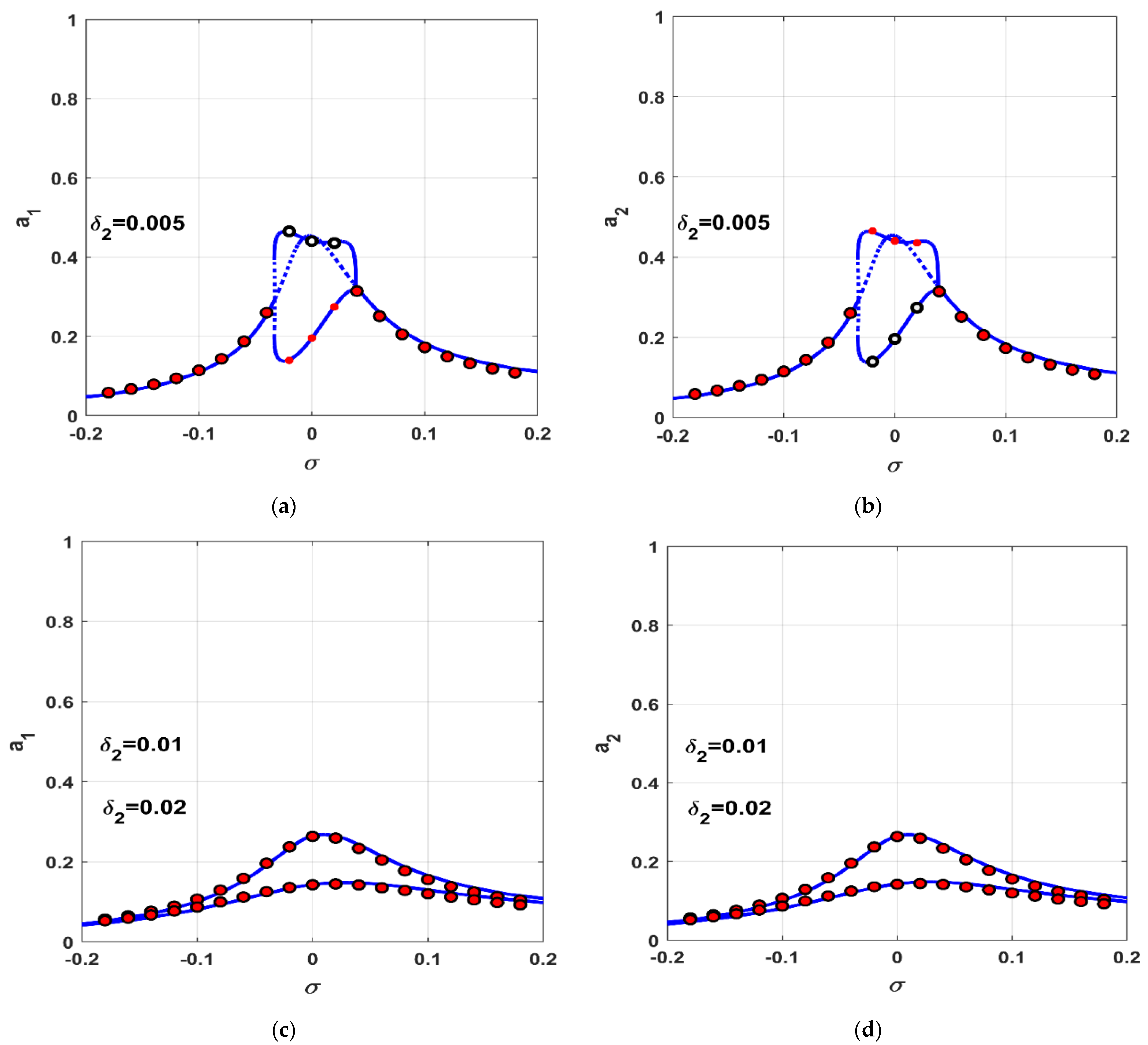
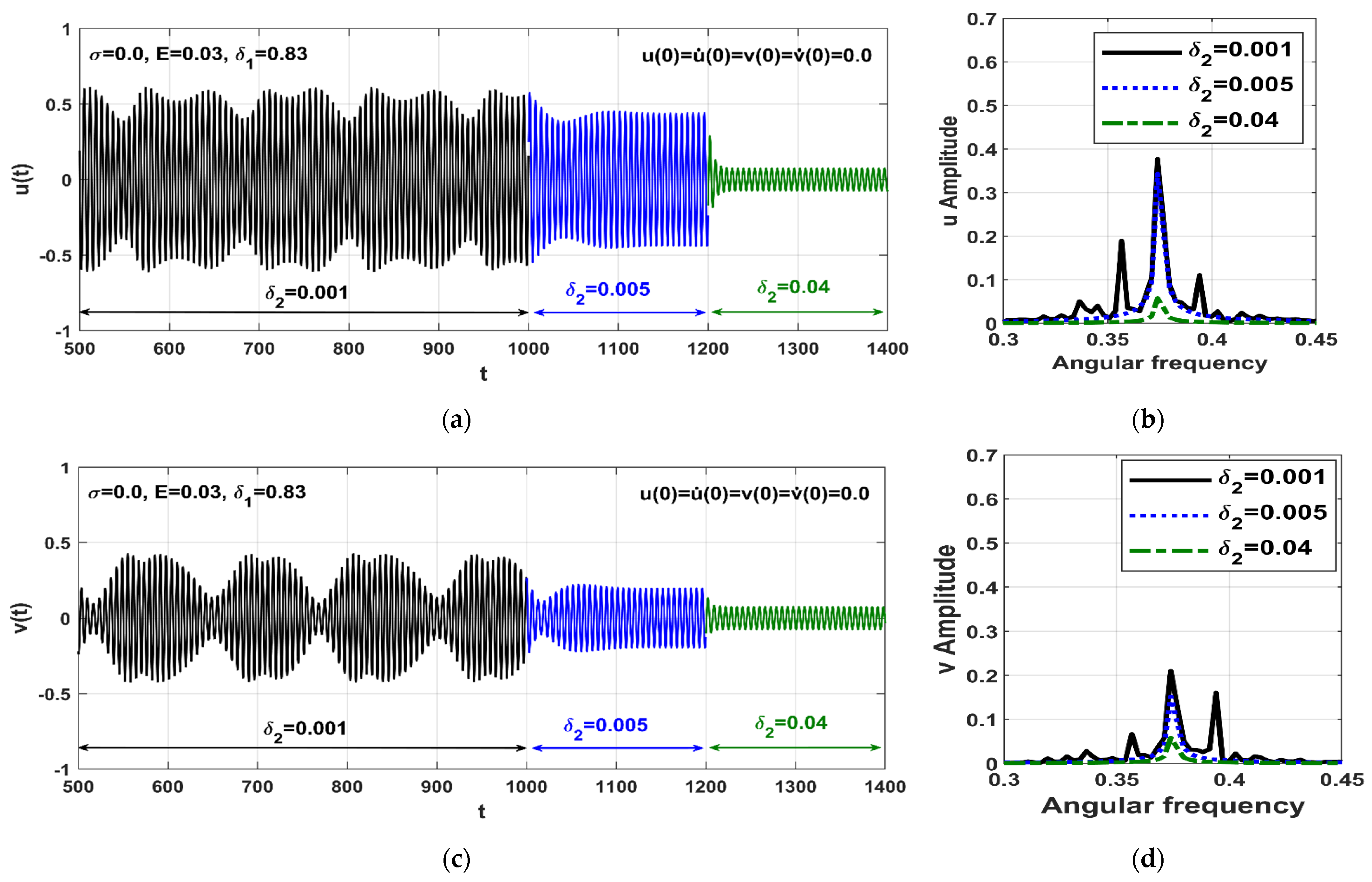
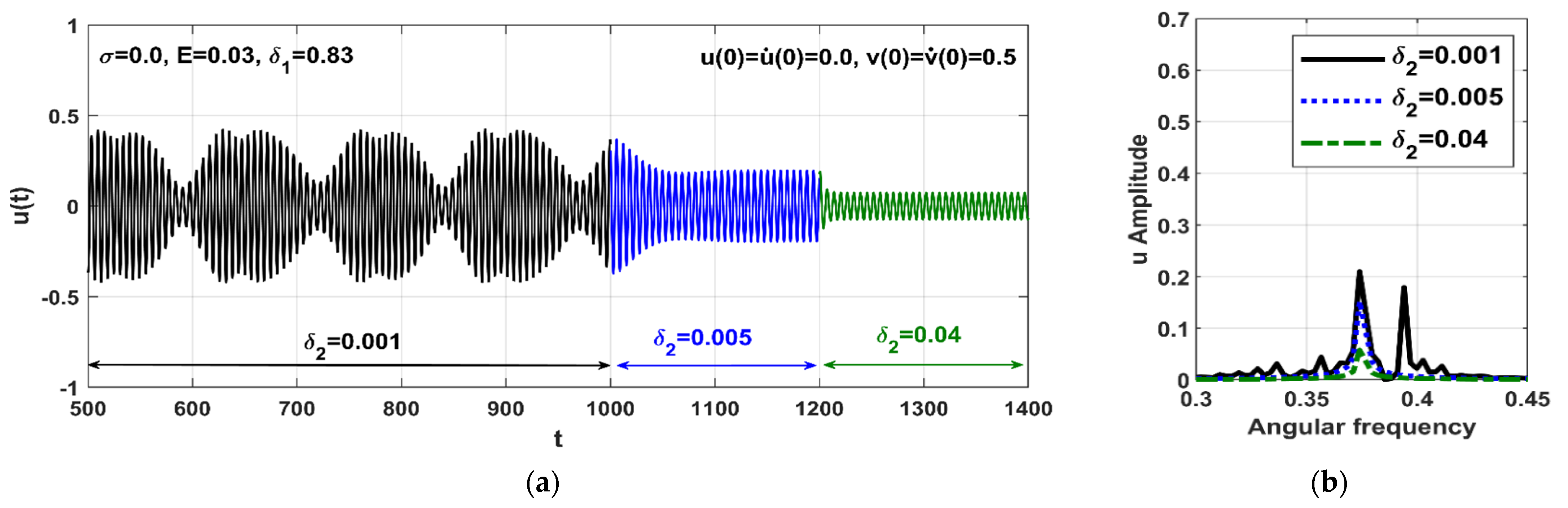
• Despite that the vibration control efficiency of the eight-pole magnetic actuator is higher than that of the four-pole magnetic actuator [24,25,26,27,28], it may destabilize the stable motion and force the Jeffcott system to oscillate with a quasi-periodic or chaotic motion if the control parameters (${\delta }_1$ and ${\delta }_2$) have not selected properly, as in Figure 7, Figure 8, Figure 9 and Figure 10. However, that is not the case with the four-pole actuator as reported in refs [24,25,26,27,28].
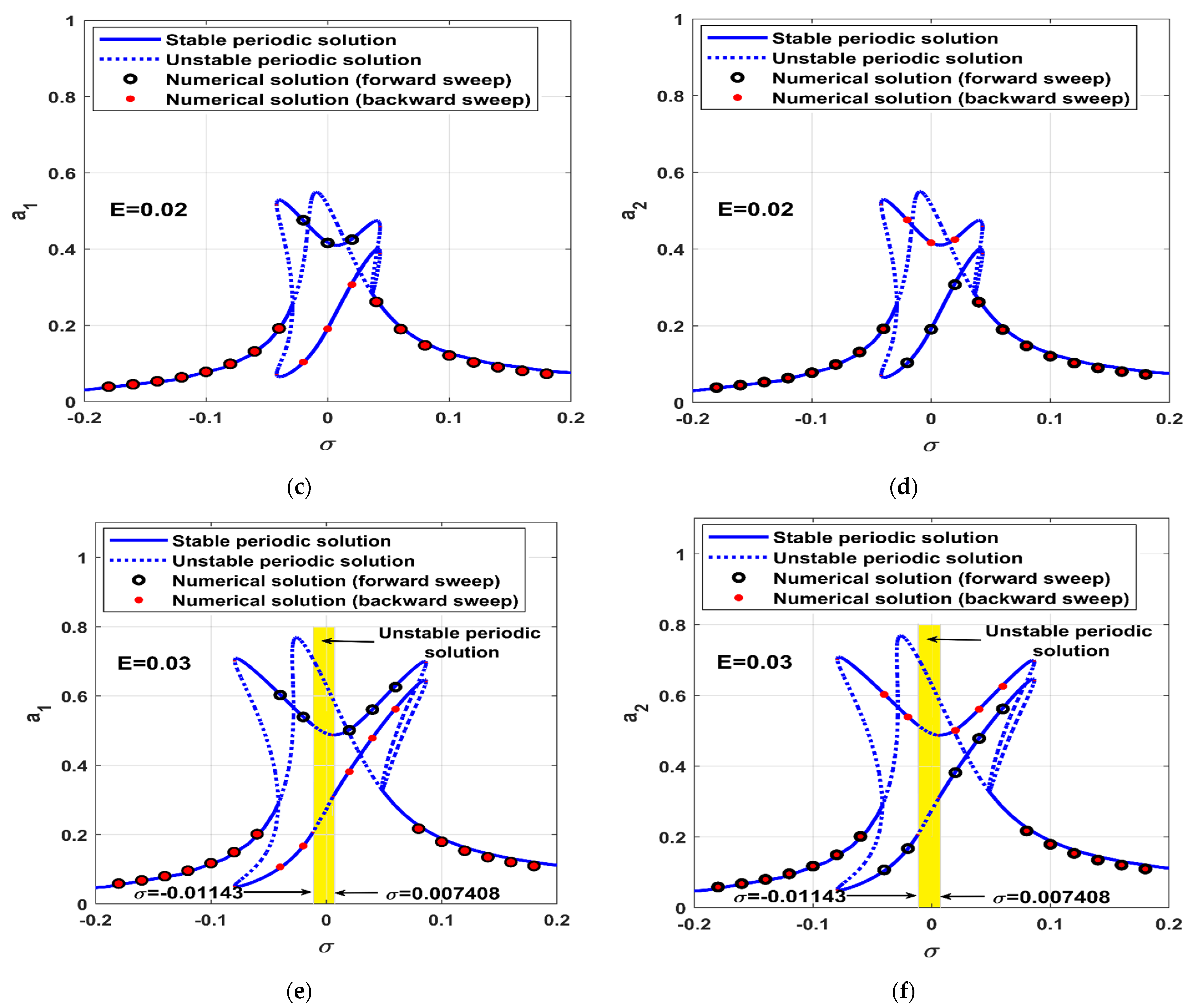
• The controlled Jeffcott system has symmetric bifurcation characteristics and asymmetric oscillation in both the horizontal and the vertical direction regardless of the shaft eccentricity and the rotor spinning speed.

References

1. Yamamoto, T. On the vibrations of a shaft supported by bearings having radial clearances. Trans. Jpn. Soc. Mech. Eng. 1955, 21, 186–192. [Google Scholar] [CrossRef] [Green Version]
2. Ehrich, F.F. High-order subharmonic response of highspeed rotors in bearing clearance. ASME J. Vib. Acoust. Stress. Reliab. Des. 1988, 110, 9–16. [Google Scholar] [CrossRef]
3. Ganesan, R. Dynamic response and stability of a rotor support system with non-symmetric bearing clearances. Mech. Mach. Theory 1996, 31, 781–798. [Google Scholar] [CrossRef]
4. Chávez, J.P.; Hamaneh, V.V.; Wiercigroch, M. Modelling and experimental verification of an asymmetric Jeffcott rotor with radial clearance. J. Sound Vib. 2015, 334, 86–97. [Google Scholar] [CrossRef]
5. Yamamoto, T.; Ishida, Y. Theoretical discussions on vibrations of a rotating shaft with non-linear spring characteristics. Arch. Appl. 1977, 46, 125–135. [Google Scholar]
6. Ishida, Y.; Ikeda, T.; Yamamoto, T.; Murakami, S. Vibration of a rotating shaft with non-linear spring characteristics during acceleration through a critical speed. 2nd report. A critical speed of a 1/2-order subharmonic oscillation. Trans. Jpn. Soc. Mech. Eng. 1986, 55, 636–643. [Google Scholar] [CrossRef] [Green Version]
7. Ishida, Y.; Ikeda, T.; Yamamoto, T.; Murakami, S. Nonstationary vibration of a rotating shaft with non-linear spring characteristics during acceleration through a critical speed. A critical speed of a 1/2-order subharmonic oscillation. JSME Int. J. 1989, 32, 575–584. [Google Scholar]
8. Adiletta, G.; Guido, A.R.; Rossi, C. Non-periodic motions of a Jeffcott rotor with non-linear elastic restoring forces. Non-Linear Dyn. 1996, 11, 37–59. [Google Scholar] [CrossRef] [Green Version]
9. Kim, Y.; Noah, S. Quasi-periodic response and stability analysis for a non-linear Jeffcott rotor. J. Sound Vib. 1996, 190, 239–253. [Google Scholar] [CrossRef]
10. Ishida, Y.; Inoue, T. internal resonance phenomena of the Jeffcott rotor with non-linear spring characteristics. J. Vib. Acoust. 2004, 126, 476–484. [Google Scholar] [CrossRef]
11. Cveticanin, L. Free vibration of a Jeffcott rotor with pure cubic non-linear elastic property of the shaft. Mech. Mach. Theory 2005, 40, 1330–1344. [Google Scholar] [CrossRef]
12. Yabuno, H.; Kashimura, T.; Inoue, T.; Ishida, Y. Non-linear normal modes and primary resonance of horizontally supported Jeffcott rotor. Non-Linear Dyn. 2011, 66, 377–387. [Google Scholar] [CrossRef]
13. Saeed, N.A.; El-Gohary, H.A. On the non-linear oscillations of a horizontally supported Jeffcott rotor with a non-linear restoring force. Non-Linear Dyn. 2017, 88, 293–314. [Google Scholar] [CrossRef]
14. Han, Q.; Chu, F. Parametric instability of a Jeffcott rotor with rotationally asymmetric inertia and transverse crack. Non-Linear Dyn. 2013, 73, 827–842. [Google Scholar] [CrossRef]
15. Saeed, N.A.; Eissa, M. Bifurcation analysis of a transversely cracked non-linear Jeffcott rotor system at different resonance cases. Int. J. Acoust. Vib. 2019, 24, 284–302. [Google Scholar] [CrossRef]
16. Saeed, N.A.; Mohamed, M.S.; Elagan, S.K. Periodic, Quasi-Periodic, and Chaotic Motions to Diagnose a Crack on a Horizontally Supported Non-linear Rotor System. Symmetry 2020, 12, 2059. [Google Scholar] [CrossRef]
17. Chang-Jian, C.-W.; Chen, C.-K. Chaos of rub–impact rotor supported by bearings with non-linear suspension. Tribol. Int. 2009, 42, 426–439. [Google Scholar] [CrossRef]
18. Chang-Jian, C.-W.; Chen, C.-K. Non-linear analysis of a rub-impact rotor supported by turbulent couple stress fluid film journal bearings under quadratic damping. Non-Linear Dyn. 2009, 56, 297–314. [Google Scholar] [CrossRef]
19. Khanlo, H.M.; Ghayour, M.; Ziaei-Rad, S. Chaotic vibration analysis of rotating, flexible, continuous shaft-disk system with a rub-impact between the disk and the stator. Commun. Non-Linear Sci. Numer. Simulat. 2011, 16, 566–582. [Google Scholar] [CrossRef]
20. Chen, Y.; Liu, L.; Liu, Y.; Wen, B. Non-linear Dynamics of Jeffcott Rotor System with Rub-Impact Fault. Adv. Eng. Forum 2011, 2–3, 722–727. [Google Scholar] [CrossRef] [Green Version]
21. Wang, J.; Zhou, J.; Dong, D.; Yan, B.; Huang, C. Non-linear dynamic analysis of a rub-impact rotor supported by oil film bearings. Arch. Appl. Mech. 2013, 83, 413–430. [Google Scholar] [CrossRef]
22. Khanlo, H.M.; Ghayour, M.; Ziaei-Rad, S. The effects of lateral–torsional coupling on the non-linear dynamic behavior of a rotating continuous flexible shaft–disk system with rub–impact. Commun. Non-Linear Sci. Numer. Simulat. 2013, 18, 1524–1538. [Google Scholar] [CrossRef]
23. Hu, A.; Hou, L.; Xiang, L. Dynamic simulation and experimental study of an asymmetric double-disk rotor-bearing system with rub-impact and oil-film instability. Non-Linear Dyn. 2016, 84, 641–659. [Google Scholar] [CrossRef]
24. Saeed, N.A.; El-Bendary, S.I.; Sayed, M.; Mohamed, M.S.; Elagan, S.K. On the oscillatory behaviours and rub-impact forces of a horizontally supported asymmetric rotor system under position-velocity feedback controller. Lat. Am. J. Solids Struct. 2021, 18, e349. [Google Scholar] [CrossRef]
25. Saeed, N.A.; Awwad, E.M.; Maarouf, A.; Farh, H.M.H.; Alturki, F.A.; Awrejcewicz, J. Rub-impact force induces periodic, quasiperiodic, and chaotic motions of a controlled asymmetric rotor system. Shock. Vib. 2021, 2021, 1800022. [Google Scholar] [CrossRef]
26. Ishida, Y.; Inoue, T. Vibration Suppression of non-linear rotor systems using a dynamic damper. J. Vib. Control. 2007, 13, 1127–1143. [Google Scholar] [CrossRef]
27. Saeed, N.A.; Kamel, M. Non-linear PD-controller to suppress the non-linear oscillations of horizontally supported Jeffcott-rotor system. Int. J. Non-Linear Mech. 2016, 87, 109–124. [Google Scholar] [CrossRef]
28. Saeed, N.A.; Awwad, E.M.; El-Meligy, M.A.; Nasr, E.S.A. Sensitivity analysis and vibration control of asymmetric non-linear rotating shaft system utilizing 4-pole AMBs as an actuator. Eur. J. Mech. A/Solids 2021, 86, 104145. [Google Scholar] [CrossRef]
29. Ji, J.C. Dynamics of a Jefcott rotor-magnetic bearing system with time delays. Int. J. Non-Linear Mech. 2003, 38, 1387–1401. [Google Scholar] [CrossRef]
30. Xiu-yan, X.; Wei-hua, J. Singularity analysis of Jeffcott rotor-magnetic bearing with time delays. Appl. Math. J. Chin. Univ. 2012, 27, 419–427. [Google Scholar]
31. El-Shourbagy, S.M.; Saeed, N.A.; Kamel, M.; Raslan, K.R.; Abouel Nasr, E.; Awrejcewicz, J. On the Performance of a Non-linear Position-Velocity Controller to Stabilize Rotor-Active Magnetic-Bearings System. Symmetry 2021, 13, 2069. [Google Scholar] [CrossRef]
32. Saeed, N.A.; Awrejcewicz, J.; Mousa, A.A.A.; Mohamed, M.S. ALIPPF-Controller to Stabilize the Unstable Motion and Eliminate the Non-Linear Oscillations of the Rotor Electro-Magnetic Suspension System. Appl. Sci. 2022, 12, 3902. [Google Scholar] [CrossRef]
33. Saeed, N.A.; Mohamed, M.S.; Elagan, S.K.; Awrejcewicz, J. Integral Resonant Controller to Suppress the Non-linear Oscillations of a Two-Degree-of-Freedom Rotor Active Magnetic Bearing System. Processes 2022, 10, 271. [Google Scholar] [CrossRef]
34. Saeed, N.A.; Awwad, E.M.; El-Meligy, M.A.; Nasr, E.S.A. Radial versus cartesian control strategies to stabilize the non-linear whirling motion of the six-pole rotor-AMBs. IEEE Access 2020, 8, 138859–138883. [Google Scholar] [CrossRef]
35. El-Shourbagy, S.M.; Saeed, N.A.; Kamel, M.; Raslan, K.R.; Aboudaif, M.K.; Awrejcewicz, J. Control Performance, Stability Conditions, and Bifurcation Analysis of the Twelve-Pole Active Magnetic Bearings System. Appl. Sci. 2021, 11, 10839. [Google Scholar] [CrossRef]
36. Heindel, S.; Becker, F.; Rinderknecht, S. Unbalance and resonance elimination with active bearings on a Jeffcott Rotor. Mech. Syst. Signal Process. 2017, 85, 339–353. [Google Scholar] [CrossRef]
37. Heindel, S.; Müller, P.C.; Rinderknecht, S. Unbalance and resonance elimination with active bearings on general rotors. J. Sound Vib. 2018, 431, 422–440. [Google Scholar] [CrossRef]
38. Heindel, S. Unbalance and Resonance Elimination on General Rotors with Active Bearings. Ph.D. Thesis, Department of Mechanical Engineering, The Technical University of Darmstadt, Darmstadt, Germany, 2017. [Google Scholar]
39. Ishida, Y.; Yamamoto, T. Linear and Non-Linear Rotordynamics: A Modern Treatment with Applications, 2nd ed.; Wiley-VCH Verlag GmbH & Co., KGaA: New York, NY, USA, 2012. [Google Scholar] [CrossRef]
40. Schweitzer, G.; Maslen, E.H. Magnetic Bearings: Theory, Design, and Application to Rotating Machinery; Springer: Berlin/Heidelberg, Germany, 2009. [Google Scholar] [CrossRef]
41. Nayfeh, A.H.; Mook, D.T. Non-Linear Oscillations; Wiley: New York, NY, USA, 1995. [Google Scholar] [CrossRef]
42. Nayfeh, A.H. Resolving Controversies in the Application of the Method of Multiple Scales and the Generalized Method of Averaging. Non-Linear Dyn. 2005, 40, 61–102. [Google Scholar] [CrossRef]
43. Slotine, J.-J.E.; Li, W. Applied Non-Linear Control; Prentice Hall: Englewood Cliffs, NJ, USA, 1991. [Google Scholar]
44. Yang, W.Y.; Cao, W.; Chung, T.; Morris, J. Applied Numerical Methods Using Matlab; John Wiley & Sons, Inc.: Hoboken, NJ, USA, 2005. [Google Scholar]
Figure 1. Uncontrolled Jeffcott rotor system.
Applsci 12 06688 g001
Figure 2. (a) Jeffcott-rotor system and magnetic bearings actuator at the nominal position. (b) Jeffcott-rotor system and magnetic bearings actuator at small displacements x ( τ ) and y ( τ ) away from the nominal position.
Applsci 12 06688 g002
Figure 3. Schematic diagram to show the interconnection between the Jeffcott-rotor system, magnetic bearings actuator, and control algorithm.
Applsci 12 06688 g003
Figure 4. σ —response curve of the uncontrolled Jeffcott rotor at various values of the shaft eccentricity E : (a) oscillation amplitude in X —direction ( a 1 ) versus σ , and (b) oscillation amplitude in Y —direction ( a 2 ) versus σ .
Applsci 12 06688 g004
Figure 5. E —response curves of the uncontrolled Jeffcott rotor at various values of σ : (a) oscillation amplitude in X —direction ( a 1 ) versus the eccentricity ( E ), and (b) oscillation amplitude in Y —direction ( a 2 ) the eccentricity ( E ).
Applsci 12 06688 g005
Figure 6. σ —response curve of the controlled Jeffcott rotor (i.e., δ 1 = 0.83 , and δ 2 = 0.002 ) at three different values of the shaft eccentricity E : (a,b) oscillation amplitudes ( a 1 and a 2 ) versus σ when E = 0.01 , (c,d) oscillation amplitudes ( a 1 and a 2 ) versus σ when E = 0.02 , and (e,f) oscillation amplitudes ( a 1 and a 2 ) versus σ when E = 0.03 .
Applsci 12 06688 g006aApplsci 12 06688 g006b
Figure 7. E —response curve of the controlled Jeffcott rotor (i.e., δ 1 = 0.83 and δ 2 = 0.002 ) and the corresponding bifurcation diagrams at σ = 0.0 : (a,b) oscillation amplitudes ( a 1 and a 2 ) versus E when σ = 0 , and (c,d) Poincaré-map of the instantaneous oscillations u ( t ) and v ( t ) versus E when σ = 0 .
Applsci 12 06688 g007
Figure 8. Periodic time-response, Poincaré-map, and frequency-spectrum of the controlled Jeffcott-rotor according to Figure 7 (i.e., at σ = 0 ,   δ 1 = 0.83 ,   δ 2 = 0.002 ) when E = 0.02 : (a,b) the normalized temporal oscillations u ( t ) and v ( t ) in X and Y direction, (c,d) the corresponding Poincaré-map, (e,f) the corresponding frequency-spectrum.
Applsci 12 06688 g008
Figure 9. Quasi-periodic time-response, Poincaré-map, and frequency-spectrum of the controlled Jeffcott-rotor according to Figure 7 (i.e., at σ = 0 ,   δ 1 = 0.83 ,   δ 2 = 0.002 ) when E = 0.05 : (a,b) the normalized temporal oscillations u ( t ) and v ( t ) in X and Y direction, (c,d) the corresponding Poincaré-map, (e,f) the corresponding frequency-spectrum.
Applsci 12 06688 g009
Figure 10. Chaotic time-response, Poincaré-map, and frequency-spectrum of the controlled Jeffcott-rotor according to Figure 7 (i.e., at σ = 0 ,   δ 1 = 0.83 ,   δ 2 = 0.002 ) when E = 0.075 : (a,b) the normalized temporal oscillations u ( t ) and v ( t ) in X and Y direction, (c,d) the corresponding Poincaré-map, (e,f) the corresponding frequency-spectrum.
Applsci 12 06688 g010
Figure 11. E —response curve of the controlled Jeffcott rotor (i.e., δ 1 = 0.83 and δ 2 = 0.002 ) and the corresponding bifurcation diagrams at σ = 0.05 : (a,b) oscillation amplitudes ( a 1 and a 2 ) versus E when σ = 0 , and (c,d) Poincaré-map of the instantaneous oscillations u ( t ) and v ( t ) versus E when σ = 0 .
Applsci 12 06688 g011
Figure 12. σ —response curve of the controlled Jeffcott rotor (i.e., E = 0.03 ,   δ 1 = 0.83 , and δ 2 = 0.002 ) at the negative and positive non-linear stiffness coefficient ( λ ): (a,b) oscillation amplitudes ( a 1 and a 2 ) versus σ when λ = 0.3 , and (c,d) oscillation amplitudes ( a 1 and a 2 ) versus σ when λ = 0.3 .
Applsci 12 06688 g012
Figure 13. σ —response curve of the controlled Jeffcott rotor (i.e., E = 0.03 ,   λ = 0.05 , and δ 2 = 0.002 ) at two different value of the proportional gain δ 1 : (a,b) oscillation amplitudes ( a 1 and a 2 ) versus σ when δ 1 = 0.85 , and (c,d) oscillation amplitudes ( a 1 and a 2 ) versus σ when δ 1 = 0.8 .
Applsci 12 06688 g013
Figure 14. Time-response and the corresponding frequency-spectrum of the controlled Jeffcott-rotor according to Figure 13 when σ = 0.1 ,   E = 0.03 ,   λ = 0.05 ,   δ 2 = 0.002 when decreasing online the proportional gain from δ 1 = 0.85 to δ 1 = 0.8 at time t = 700 : (a,b) the normalized temporal oscillations u ( t ) and the corresponding frequency spectrum in X direction, (c,d) the normalized temporal oscillations v ( t ) and the corresponding frequency spectrum in Y direction.
Applsci 12 06688 g014
Figure 15. σ —response curve of the controlled Jeffcott rotor (i.e., E = 0.03 ,   λ = 0.05 , and δ 1 = 0.83 ) at three different value of the derivative gain δ 2 : (a,b) oscillation amplitudes ( a 1 and a 2 ) versus σ when δ 2 = 0.005 , and (c,d) oscillation amplitudes ( a 1 and a 2 ) versus σ when δ 2 = 0.01 ,   0.02 .
Applsci 12 06688 g015
Figure 16. δ 2 —response curve of the controlled Jeffcott rotor (i.e., E = 0.03 ,   λ = 0.05 , and δ 1 = 0.83 ): (a) oscillation amplitude a 1 versus δ 2 when σ = 0 , and (b) oscillation amplitude a 2 versus δ 2 when σ = 0 .
Applsci 12 06688 g016
Figure 17. Time-response and the corresponding frequency-spectrum of the controlled Jeffcott-rotor according to Figure 16 at the initial conditions u ( 0 ) = u ˙ ( 0 ) = v ( 0 ) = v ˙ ( 0 ) = 0 and parameter values σ = 0 ,   E = 0.03 ,   λ = 0.05 ,   δ 1 = 0.83 when increasing the derivative gain online from δ 2 = 0.001 to δ 2 = 0.005 at time t = 1000 , and then from δ 2 = 0.005 to δ 2 = 0.04 at   t = 1200 : (a,b) the normalized temporal oscillations u ( t ) and the corresponding frequency spectrum in X direction, (c,d) the normalized temporal oscillations v ( t ) and the corresponding frequency spectrum in Y direction.
Applsci 12 06688 g017
Figure 18. Time-response and the corresponding frequency-spectrum of the controlled Jeffcott-rotor according to Figure 16 at the initial conditions u ( 0 ) = u ˙ ( 0 ) = 0 ,   v ( 0 ) = v ˙ ( 0 ) = 0.5 and parameter values σ = 0 ,   E = 0.03 ,   λ = 0.05 ,   δ 1 = 0.83 when increasing the derivative gain online from δ 2 = 0.0.001 to δ 2 = 0.005 at time t = 1000 , and then from δ 2 = 0.005 to δ 2 = 0.04 at   t = 1200 : (a,b) the normalized temporal oscillations u ( t ) and the corresponding frequency spectrum in X direction, (c,d) the normalized temporal oscillations v ( t ) and the corresponding frequency spectrum in Y direction.
Applsci 12 06688 g018aApplsci 12 06688 g018b
Figure 19. Stability charts of the controlled Jeffcott rotor in E δ 2 plane when λ = 0.05 ,   δ 1 = 0.83 , and δ 2 = 0.002 : (a) periodic and aperiodic solutions regions in E δ 2 plane when σ = 0 , (b) periodic and aperiodic solutions regions in E δ 2 plane when σ = 0.05 .
Applsci 12 06688 g019
Figure 20. σ —response curve of the studied Jeffcott rotor system before control and after optimal control (i.e., δ 1 = 0.83 and δ 2 = 0.02 ): (a) oscillation amplitude a 1 versus σ when E = 0.03 , and (b) oscillation amplitude a 2 versus σ when E = 0.03 .
Applsci 12 06688 g020
Figure 21. Time-response and the corresponding frequency-spectrum of the Jeffcott-rotor system before and after control according to Figure 20 at σ = 0.0 ,   E = 0.03 ,   λ = 0.05 ,   δ 1 = 0.83 ,   δ 2 = 0.02 when turning the controller on at time t = 600 : (a,b) the normalized temporal oscillations u ( t ) and the corresponding frequency spectrum in X direction, (c,d) the normalized temporal oscillations v ( t ) and the corresponding frequency spectrum in Y direction.
Applsci 12 06688 g021
Figure 22. E —response curve of the studied Jeffcott rotor system before control and after optimal control (i.e., δ 1 = 0.83 and δ 2 = 0.02 ): (a) oscillation amplitude a 1 versus E when σ = 0 , and (b) oscillation amplitude a 2 versus E when σ = 0 .
Applsci 12 06688 g022
Figure 23. Time-response and the corresponding frequency-spectrum of the Jeffcott-rotor system before and after control according to Figure 22 at σ = 0.0 ,   E = 0.075 ,   λ = 0.05 ,   δ 1 = 0.83 ,   δ 2 = 0.02 when turning the controller on at time t = 600 : (a,b) the normalized temporal oscillations u ( t ) and the corresponding frequency spectrum in X direction, (c,d) the normalized temporal oscillations v ( t ) and the corresponding frequency spectrum in Y direction.
Applsci 12 06688 g023
Publisher’s Note: MDPI stays neutral with regard to jurisdictional claims in published maps and institutional affiliations.