China’s Water Intensity Factor Decomposition and Water Usage Decoupling Analysis

Abstract

As the most populous country in the world, China has a great shortage pressure of water resources. With the acceleration of urbanization, China’s water usage in different sectors will change significantly in next few years. In order to investigate the main reasons behind water usage change in China, the Logarithmic Mean Divisia Index (LMDI) model was adopted in this paper from 2000 to 2020 with provincial data. Three effects, including that of technology, industrial structure, and regional scale, were analyzed. In addition, the decoupling effect between water usage and economic growth was also considered. The results show that: (1) from 2000 to 2020, the technological effect, industrial structure effect, and regional scale effect are −376.54, −89.85 and 20.66, respectively; (2) the technical effect and industrial structure effect have the greatest impact on primary industry, followed by secondary industry; (3) the technical effect is greater than the industrial structure effect in most provinces; and (4) the decoupling state gradually changes from weak decoupling to strong decoupling. In the future, the key policy recommendations for water saving are the following: (1) technological innovation has the most efficient effect on the reduction of water usage in China, and (2) the optimization of industrial structure can be helpful in water-saving in the future.

1. Introduction

China is one of the countries with the most serious water shortage pressures in the world [1,2,3]. Besides, the weak awareness of water saving, uneven distribution of water resources, rapid population growth, increasing water usage of residents, and climate change have all aggravated the tensions surrounding water resources in China [4,5]. With the rapid development of modern industry and the accelerating process of urbanization, the demand for water resources in different sectors will change greatly, and access to water will become an important factor restricting China’s economic development [6,7].

In the last 20 years, China’s water usage structure has changed significantly in line with economic development. The water usage in China has been divided into three industries. The primary industry category mainly includes agriculture, forestry, and animal husbandry and fisheries. The secondary industry category mainly refers to mining, manufacturing, and construction. The tertiary industries include everything not contained within the primary and secondary industries, including the service industry, transportation, accommodation and catering, finance, real estate, culture and sports, public administration, and social security [8,9]. The water usage in primary industry showed a downward trend, and the water usage in secondary industry increased first and then decreased [10,11,12]. Water usage in tertiary industry continued to rise at a rapidly increasing rate, which was 15% in 2020 [13,14]. Therefore, it is of great significance for the sustainable management of water resources to investigate the driving factors behind China’s water intensity [15].

A series of publications have calculated the single resource intensity at national level, the city level, and certain industry levels. Some researchers even considered the resource intensity of overall resources in the world or in a certain country.

A series of publications regarding driving factors in different resources have been conducted by previous researchers, including structural decomposition analysis (SDA), granger causality test, and the Logarithmic Mean Divisia Index (LMDI) model. Most of the existing studies using SDA were based on the monetary I–O tables, which require a considerable amount of sector data, and the research scope is mainly in a national level [16,17,18]. While the Granger causality test is only a statistical estimation, not a real causality, which cannot be used as the basis for affirming or denying causality [19,20,21]. Therefore, the LMDI model was adopted in this paper.

The LMDI model is a factor decomposition method that does not generate residual error [22]. The application of LMDI is essentially for resources and the environment, such as carbon emissions, energy, land, and water resources [23,24,25,26,27,28]. At present, LMDI research on water resources has calculated the driving factors at national level or the city level [29,30,31,32,33,34,35]. The LMDI method in water resources research was mainly broken down into population scale effect, economic development effect, domestic intensity effect, production intensity, and industrial structural effect [36]. However, as the world’s most populous country with serious water usage pressure, there is a shortage of research on the drivers of change in China’s water intensity at industrial level with provincial data.

Based on the data of water usage, GDP, and the added value of various industries in different provinces of China from 2000 to 2020, the LMDI model was used to analyze the potential factors affecting the change of water usage within various industries. Three effects, including the technical effect, industrial structure effect, and regional scale effect will be adopted. Besides, these three effects will be applied in each province and each industry in China. The decomposition model can measure the contribution of various factors to water intensity, while it cannot directly measure the decoupling state between economic growth and water usage, and the actual decoupling situation under different policies [37]. The Tapio method is then used for decoupling analysis between water usage and GDP. Finally, the most efficient water-saving methods will also be discussed.

2. Materials and Methods

2.1. Logarithmetic Mean Divisia Index Model

In order to analyze the influence of technological progress, regional scale, industrial structure, and other factors on the water usage change of different industries in China, it is beneficial to analyze the driving factors of water usage in China by using the LMDI proposed by Ang [38]. This method has the advantages of zero value and complete decomposition, and can be completely decomposed [39,40,41].

Water usage index can be expressed by absolute quantity and relative quantity. The absolute quantity refers to total water usage, and the relative quantity refers to the water usage per unit of economic output, that is, water intensity. It reflects the utilization efficiency of water resources, which is influenced by economic growth, technological progress, industrial structure, regional scale, and policy factors. According to the definition of water intensity, it can be expressed as:

$$w={\displaystyle \sum }_i{\displaystyle \sum }_j\frac{W_{ij}}{G_{ij}}$$

(1)

where w is the water intensity (cubic meters/10 thousand CNY); W_ij is the water usage (cubic meters) of the jth industry in the ith province; G_ij is the gross output value (10 thousand CNY) of the jth industry in the ith province.

According to LMDI analysis framework, by analyzing the influence of each effect on water intensity, we can construct Equation (2) as follows:

$$w={{\displaystyle \sum }}_i{{\displaystyle \sum }}_j\frac{W_{ij}}{G}={{\displaystyle \sum }}_i{{\displaystyle \sum }}_j\frac{W_{ij}}{G_{ij}}\times \frac{G_{ij}}{G_i}\times \frac{G_i}{G}={{\displaystyle \sum }}_i{{\displaystyle \sum }}_j{q}_{ij}{r}_{ij}{s}_i$$

(2)

where w is the water intensity, W_ij is the total water usage of the jth industry in the ith province, G_ij is the gross national product of the jth industry in the ith province, G_i is the gross product of the ith province, G is the gross domestic product, q_ij is the water intensity of the jth industry in the ith province, r_ij is the proportion of the gross product of the jth industry in the gross product of the ith province, s_i is the ratio of GDP of the ith province to total GDP.

Therefore, the total effect formula of water intensity is:

$$∆tot=∆t+∆u+∆v$$

(3)

where $∆tot$ is the total effect, that is, the sum of all effects, indicating the total change of water intensity; $∆t$ refers to the technical effect, indicating the contribution of the change of resource utilization efficiency caused by technological progress to the total change of water intensity; $∆u$ refers to the industrial structure effect, indicating the contribution of industrial structure adjustment to the total change of water intensity; $∆v$ is the regional scale effect, which indicates the contribution of the ratio of regional economic output to GDP to the total change of water intensity.

The contribution of each effect is expressed as follows:

$$∆t={\displaystyle \sum }_i{\displaystyle \sum }_j\frac{\frac{W_{ij}^T}{G^T}-\frac{W_{ij}^0}{G^0}}{\ln (\frac{W_{ij}^T}{G^T})-\ln (\frac{W_{ij}^0}{G^0})}ln(\frac{q_{ij}^T}{q_{ij}^0})$$

(4)

$$∆u={\displaystyle \sum }_i{\displaystyle \sum }_j\frac{\frac{W_{ij}^T}{G^T}-\frac{W_{ij}^0}{G^0}}{\ln (\frac{W_{ij}^T}{G^T})-\ln (\frac{W_{ij}^0}{G^0})}ln(\frac{r_{ij}^T}{r_{ij}^0})$$

(5)

$$∆v={\displaystyle \sum }_i{\displaystyle \sum }_j\frac{\frac{W_{ij}^T}{G^T}-\frac{W_{ij}^0}{G^0}}{\ln (\frac{W_{ij}^T}{G^T})-\ln (\frac{W_{ij}^0}{G^0})}ln(\frac{s_{ij}^T}{s_{ij}^0})$$

(6)

The contribution rates of the three effects to the change of water intensity are $∆t/∆tot$, $∆u/∆tot$, and $∆v/∆tot$, respectively. When the positive and negative impacts of each effect are consistent with the total effect, it shows that this effect has a positive impact on the reduction of water intensity, and vice versa.

2.2. Decoupling Model

The decomposition model can be used to study the contribution of various factors to the change of water usage intensity, but it cannot directly measure the decoupling state between economy and water usage [22]. Therefore, the Tapio decoupling model is adopted [42,43,44], and the decomposition model of water usage is as follows:

$$W={\displaystyle \sum }_i{\displaystyle \sum }_j{W}_{ij}={\displaystyle \sum }_i{\displaystyle \sum }_j\frac{W_{ij}}{G_{ij}}\times \frac{G_{ij}}{G_i}\times \frac{G_i}{G}\times G$$

(7)

So as to decompose the changes of water usage into:

$$∆TOT={\displaystyle \sum }_i{\displaystyle \sum }_j∆T+∆U+∆V+∆Q$$

(8)

Among them, $∆TOT$ is the total effect of water usage, $∆T$ is the technical effect, $∆U$ is the effect of industrial structure, $∆V$ is the effect of regional scale, and $∆Q$ is the effect of output scale. The contribution of each effect is as follows:

$$∆T={\displaystyle \sum }_i{\displaystyle \sum }_j\frac{W_{ij}^T-W_{ij}^0}{ln{W}_{ij}^T-ln{W}_{ij}^0}ln(\frac{W_{ij}^T/G_{ij}^T}{W_{ij}^0/G_{ij}^0})$$

(9)

$$∆U={\displaystyle \sum }_i{\displaystyle \sum }_j\frac{W_{ij}^T-W_{ij}^0}{ln{W}_{ij}^T-ln{W}_{ij}^0}ln(\frac{G_{ij}^T/G_i^T}{G_{ij}^0/G_i^0})$$

(10)

$$∆V={\displaystyle \sum }_i{\displaystyle \sum }_j\frac{W_{ij}^T-W_{ij}^0}{ln{W}_{ij}^T-ln{W}_{ij}^0}ln(\frac{G_i^T/G^T}{G_i^0/G^0})$$

(11)

$$∆Q={\displaystyle \sum }_i{\displaystyle \sum }_j\frac{W_{ij}^T-W_{ij}^0}{ln{W}_{ij}^T-ln{W}_{ij}^0}ln\frac{G^T}{G^0}$$

(12)

Decoupling elasticity index is used to discuss the decoupling relationship between economic growth and water usage. The elastic coefficient of GDP water usage is calculated as follows:

$$\omega \left(W,G\right)=\frac{∆W/W}{∆G/G}$$

(13)

The types of decoupling can essentially be divided into coupling, decoupling, and negative decoupling. In addition, according to the elasticity coefficient, the change of water usage and the change of GDP, the decoupling types can be subdivided into eight cases (

Table 1. Types of Tapio models.

State	Type	△W	△GDP	ω	Meaning
Connection	Decline connection (DC)	−	−	(0.8, 1.2)	Water usage is declining at the same rate as the economy.
	Expansion connection (EC)	+	+	(0.8, 1.2)	Water usage is increasing at the same rate as the economy.
Decoupling	Decline decoupling (DD)	−	−	(1.2, +∞)	Water usage is declining faster than the economic recession.
	Strong decoupling (SD)	−	+	(−∞, 0)	Economic growth is accompanied by a decline in water usage.
	Weak Decoupling (WD)	+	+	(0, 0.8)	The growth rate of water usage is slower than that of economy.
Negative decoupling	Weak negative decoupling (WND)	−	−	(0, 0.8)	The rate of water usage reduction is slower than the rate of economic recession.
	Strong negative decoupling (SND)	+	−	(−∞, 0)	Water usage is increasing but the economy is declining.
	Expansion negative decoupling (END)	+	+	(1.2, +∞)	The water usage growth rate is lower than the economic growth rate.

) [45].

The decoupling elasticity index can be used to calculate the decoupling relationship between economic growth and water usage, but it cannot help to investigate the specific factors that affect the decoupling state. The LMDI model can be used to analyze the influence of various factors on water usage, but it cannot be used to analyze the decoupling effect between economic growth and water usage. Combining the LMDI model with the Tapio decoupling model, a decoupling effort index model is constructed:

$$∆W_{US}=∆TOT-{\displaystyle \sum }_i{\displaystyle \sum }_j∆Q={\displaystyle \sum }_i{\displaystyle \sum }_j∆T+∆U+∆V$$

(14)

where $∆W_{US }$indicates the government’s efforts to save water, and refers to various measures taken by the government to reduce water usage in the process of economic development, such as improving production technology, adjusting industrial structure, and expanding regional scale.

The decoupling effort indicators are constructed as follows:

$$D_i=-\frac{∆W_{US}}{{{\displaystyle \sum }}_i{{\displaystyle \sum }}_j∆Q}$$

(15)

where D_i is the total decoupling effect of water usage. When D_i > 1, it indicates a strong decoupling effect. When D_i < 1, it indicates a weak decoupling effect. When D_i < 0, it means there is no decoupling effect.

2.3. Date

The data used in this study are the water usage and industrial added value of three major industries in each province of China from 2000 to 2020. All the data in this paper come from the Water Resources Bulletin issued by China’s Ministry of Water Resources from 2000 to 2020 and the National Bureau of Statistics [46,47].

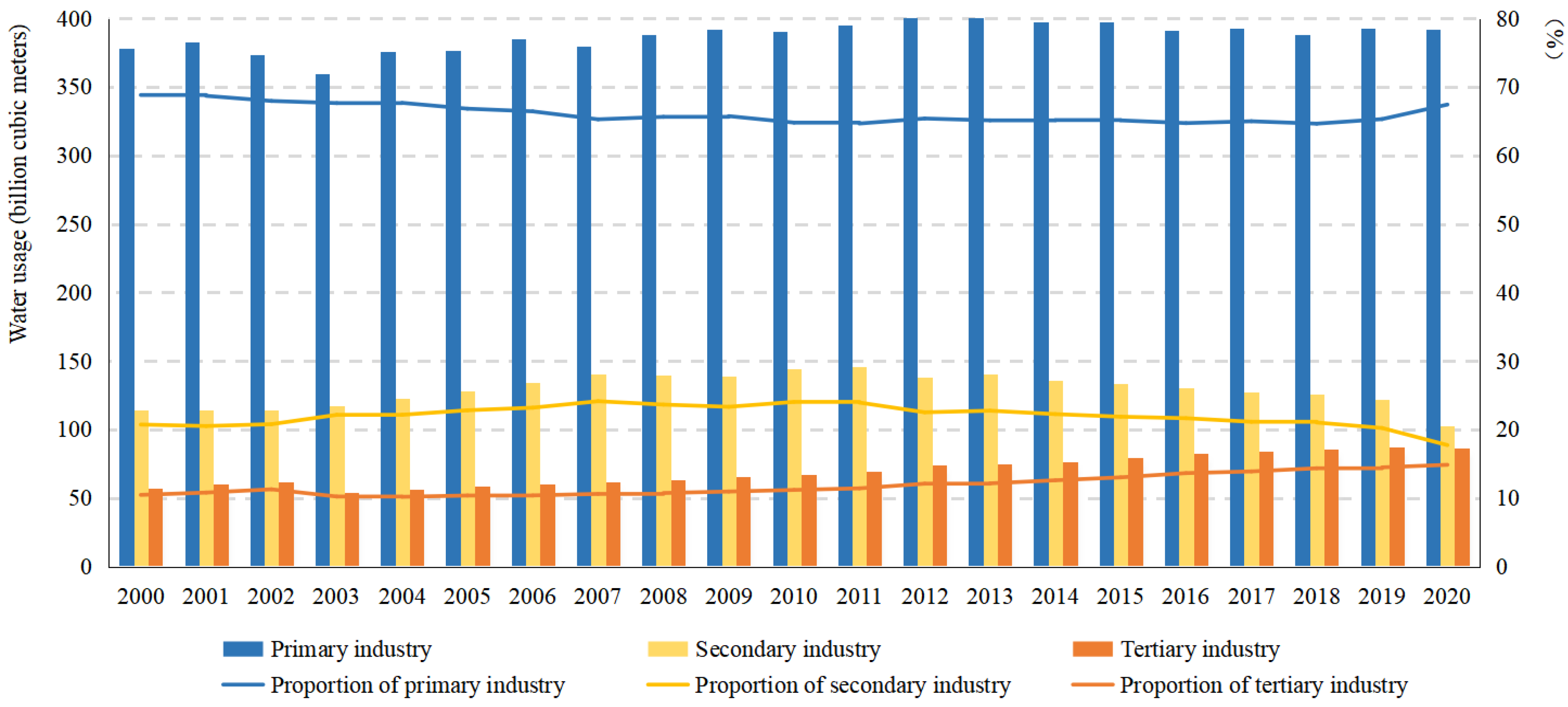
From 2000 to 2013, China’s total annual water usage increased from 549.752 billion cubic meters to 618.394 billion cubic meters, before the water usage showed a decreasing trend. The water usage of primary industry contributes most to the total water usage and remains stable with approximately 400 billion cubic meters per year. While secondary industry is a more minor user of water in China, and it has a trend of first increasing and then decreasing. The water usage of tertiary industry continues to rise, from 57.492 billion cubic meters in 2000 to 86.310 billion cubic meters in 2020 (Figure 1).

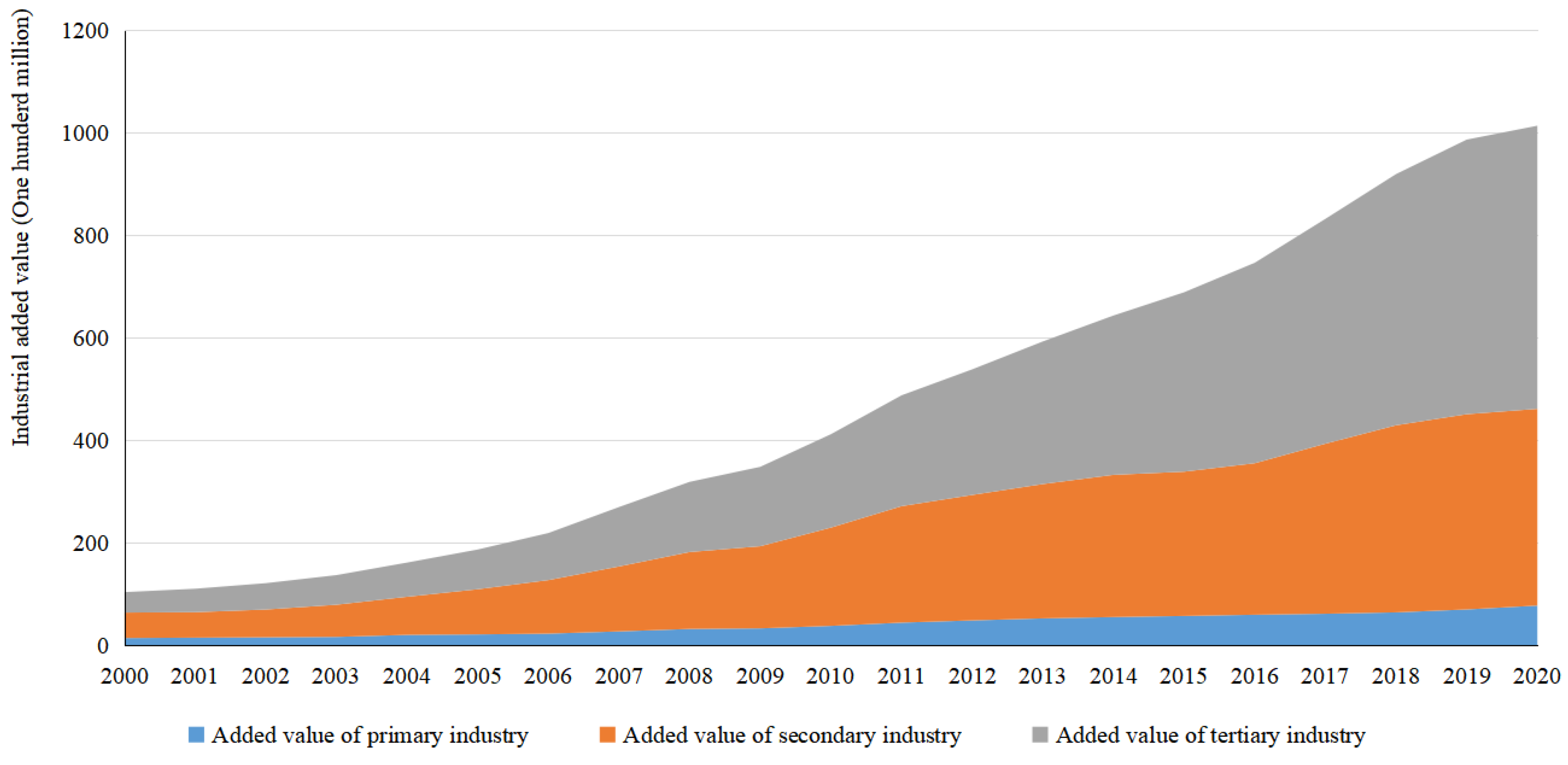
The added value in each industry of the past 20 years is shown in Figure 2. China’s economy maintains a high speed of development from 2000 to 2020, so the added value in each industry increases continually. The fastest growth occurs in tertiary industry, with an average annual growth rate of 0.07%, which demonstrates that China’s economy has gradually shifted into tertiary industry.

3. Results

3.1. Water Intensity and Factor Decomposition Analysis

3.1.1. Analysis of Decomposition Effect in Each Year

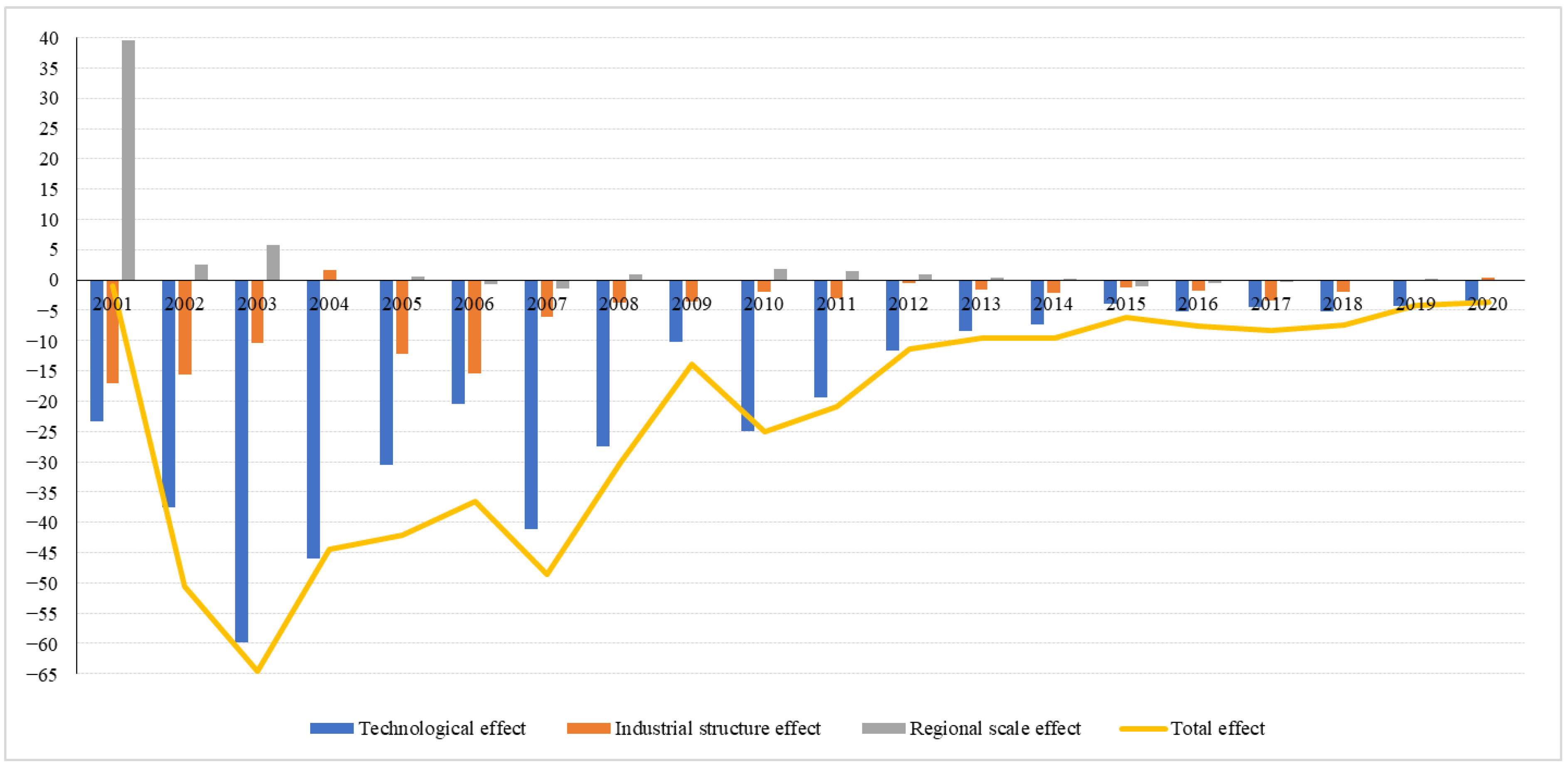
According to Equations (3)–(6), three effects and their respective contribution rates from 2000 to 2020 are shown in Figure 3. The total effect of each year is negative, indicating that the water intensity is decreasing year by year, signaling water saving considerations. The total effect from 2002 to 2003 was the smallest, with value of −64.50.

Technical effects in the last 20 years are negative and the technical effect contribution rate is the largest among three effects, indicating it has an inhibitory impact on the water intensity, while technological innovation is the most effective measure for water saving. The technical effect fluctuated greatly, with its largest value from 2002 to 2003 of −59.91 and highest contribution rate in 2001 of 2481.29%. For the industrial structure effect, it was negative except for 1.62 in 2003 and 0.38 in 2020, meaning that it restricted the water intensity in most years. As for for the regional scale effect, it fluctuated greatly from 2000 to 2001, reaching 39.49, and it was stable with values between −1 and 2 from 2003 to 2020.

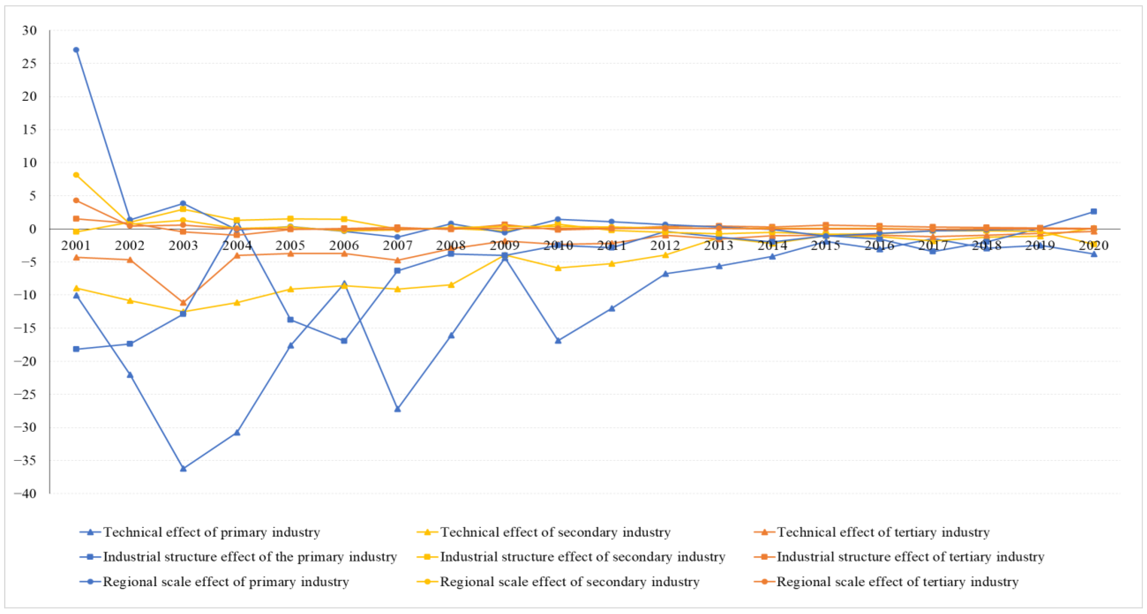
The three effects in each industry were also explored in China through the LMDI in Figure 4. The technical effects are all negative for the three industries, which means that the water intensity of the three industries all declined with technological innovation. It also fluctuated greatly before 2011, with the largest absolute value of −36.24, −12.52 and −11.15, respectively, during 2002 to 2003, then it tended to be flat. Besides, it fluctuated most within primary industry, due to the largest proportion of China’s primary industry in current water usage structure.

The industrial structure effect on the three major industries has different characteristics. In primary industry, it has increased from −18.21 to 2.63, shifting from a restriction effect to a promoting effect from 2018 to 2020. In secondary industry, it changed from strong promotion to weak promotion, and finally into a restriction effect, which is mainly attributed to the intensive management of industrial development with the increasing industry output. In tertiary industry, it remains essentially unchanged. Therefore, the industrial structure effect has restricted the water usage in China, indicating the industrial transformation in China has impacted on water usage reduction in the last 20 years.

3.1.2. Analysis of Decomposition Effect in Each Province

According to Equations (3)–(6), the three effects in each province are calculated in

Table 2. Three effects in each province in China.

Province	Technological Effect	Industrial Structure Effect	Regional Scale Effect	Total Effect
Beijing	−2.13	−1.41	0.24	−3.30
Tianjin	−1.20	−0.55	−0.05	−1.80
Hebei	−13.63	−2.69	−1.30	−17.61
Shanxi	−3.98	−0.55	0.09	−4.44
Inner Mongolia	−11.31	−3.78	1.25	−13.84
Liaoning	−8.06	−0.46	−2.69	−11.20
Jilin	−5.29	−2.75	−1.18	−9.22
Heilongjiang	−20.62	3.62	−7.05	−24.06
Shanghai	−6.20	−2.23	−0.52	−8.96
Jiangsu	−29.37	−10.35	4.59	−35.13
Zhejiang	−13.32	−4.31	0.84	−16.79
Anhui	−6.55	−9.00	2.03	−13.52
Fujian	−12.16	−3.63	1.45	−14.34
Jiangxi	−14.83	−5.38	2.71	−17.51
Shandong	−15.33	−4.35	−0.46	−20.13
Henan	−13.67	−3.87	1.15	−16.39
Hubei	−20.87	−3.82	2.68	−22.01
Hunan	−22.86	−5.70	2.65	−25.90
Guangdong	−30.22	−6.70	1.58	−35.33
Guangxi	−22.02	−3.59	1.41	−24.19
Hainan	−3.12	−0.68	0.21	−3.59
Chongqing	−4.79	−0.54	0.86	−4.46
Sichuan	−15.50	−3.49	2.25	−16.75
Guizhou	−7.78	−1.01	1.97	−6.81
Yunnan	−11.87	−1.51	1.46	−11.92
Tibet	−1.53	−1.23	0.58	−2.17
Shaanxi	−6.65	−0.99	1.33	−6.30
Gansu	−8.58	−1.20	−0.36	−10.15
Qinghai	−2.31	−0.21	0.20	−2.31
Ningxia	−6.76	−1.63	1.10	−7.29
Xinjiang	−34.05	−5.87	1.63	−38.29

. The technical effect in each province is negative with the increasing absolute value, and it means that the technical effect in each province in China has been generally improved. Besides, due to the highest average value of −12.15 in these three effects, the technical effect is a decisive factor to promote the decline of water intensity. Among all the provinces, Xinjiang have the greatest inhibitory effect with values of −34.05, and Tianjin has the smallest inhibitory effect with values of −1.20. The industrial structure effect is also negative excepted for Anhui Province in the studied areas with values between −0.21 and −10.35, and its absolute value is smaller than the technology effect. This indicates that the industrial structure transformation has taken effect.

The decomposition analysis of water intensity in each province from 2000 to 2020 is also obtained in

Table 3. Effects of various industries in various provinces.

Province	Technological Effect			Industrial Structure Effect			Regional Scale Effect
	Primary Industry	Secondary Industry	Tertiary Industry	Primary Industry	Secondary Industry	Tertiary Industry	Primary Industry	Secondary Industry	Tertiary Industry
Beijing	−0.06	−0.80	−1.27	−1.35	−0.18	0.12	0.11	0.04	0.09
Tianjin	−0.36	−0.37	−0.47	−0.56	−0.07	0.07	−0.03	−0.01	−0.01
Hebei	−9.62	−2.00	−2.00	−2.83	−0.17	0.32	−0.99	−0.15	−0.16
Shanxi	−2.25	−1.09	−0.65	−0.56	−0.04	0.05	0.06	0.02	0.01
Inner Mongolia	−9.76	−0.73	−0.82	−3.88	0.02	0.07	1.11	0.07	0.07
Liaoning	−4.89	−1.68	−1.49	−0.45	−0.26	0.25	−1.75	−0.48	−0.45
Jilin	−3.16	−1.42	−0.71	−2.81	−0.05	0.11	−0.91	−0.16	−0.11
Heilongjiang	−14.13	−5.25	−1.24	5.12	−1.80	0.29	−5.20	−1.46	−0.38
Shanghai	−0.18	−4.81	−1.21	−0.98	−1.46	0.21	−0.08	−0.36	−0.09
Jiangsu	−13.85	−11.20	−4.31	−9.91	−1.11	0.66	2.51	1.61	0.46
Zhejiang	−6.41	−4.21	−2.70	−4.37	−0.46	0.52	0.48	0.21	0.15
Anhui	−5.89	0.91	−1.56	−5.01	−4.15	0.16	1.31	0.50	0.22
Fujian	−6.07	−4.34	−1.74	−3.88	0.12	0.13	0.90	0.36	0.19
Jiangxi	−8.36	−4.80	−1.68	−5.88	0.37	0.13	1.88	0.58	0.25
Shandong	−9.83	−3.25	−2.25	−4.43	−0.35	0.44	−0.33	−0.08	−0.06
Henan	−7.24	−3.54	−2.90	−4.23	−0.14	0.50	0.76	0.21	0.18
Hubei	−11.27	−6.91	−2.68	−3.90	−0.25	0.33	1.58	0.77	0.33
Hunan	−14.12	−5.00	−3.74	−6.12	0.11	0.32	1.84	0.47	0.34
Guangdong	−15.61	−8.39	−6.22	−6.82	−0.58	0.71	0.92	0.36	0.30
Guangxi	−15.95	−3.25	−2.82	−3.80	−0.13	0.35	1.07	0.19	0.16
Hainan	−2.32	−0.33	−0.46	−0.75	0.00	0.07	0.17	0.01	0.03
Chongqing	−1.10	−2.40	−1.29	−0.61	−0.05	0.13	0.32	0.32	0.22
Sichuan	−8.17	−4.69	−2.64	−3.84	−0.02	0.36	1.48	0.41	0.36
Guizhou	−4.08	−1.92	−1.78	−1.16	−0.06	0.21	1.18	0.43	0.37
Yunnan	−8.58	−1.57	−1.72	−1.62	−0.12	0.23	1.10	0.17	0.19
Tibet	−1.25	−0.09	−0.19	−1.26	0.02	0.01	0.52	0.02	0.05
Shaanxi	−4.39	−1.24	−1.01	−1.04	0.00	0.06	0.93	0.20	0.20
Gansu	−6.51	−1.40	−0.66	−1.17	−0.11	0.09	−0.30	−0.04	−0.03
Qinghai	−1.69	−0.38	−0.24	−0.23	0.03	−0.01	0.16	0.03	0.02
Ningxia	−6.14	−0.46	−0.16	−1.64	0.00	0.01	1.00	0.06	0.03
Xinjiang	−31.70	−0.89	−1.46	−5.96	−0.04	0.12	1.54	0.03	0.05

based on Equations (3)–(6). The technical effects of all industries in each province are negative, which is consistent with Table 2, indicating the restraining effect on water usage. The value of primary industry in most provinces is the smallest, with values between −31.70 and −0.06, followed by secondary industry and tertiary industry. Because the water usage of primary industry accounts for the largest proportion of the total water usage in China, the technological progress of primary industry plays a significant role. The efficiency of technological progress in secondary industry is higher than that in tertiary industry. Moreover, the industrial structure effects of primary industry are basically negative, and it has both positive and negative values in secondary industry, with an almost positive effect on tertiary industry, indicating the greater effect of industrial transition on primary industry than that in secondary or tertiary industry. In addition, the provinces with a positive industrial structure effect of secondary industry are typically underdeveloped areas, such as Tibet, Inner Mongolia, and Qinghai, which also shows that industrial transition in underdeveloped areas needs to be improved.

3.2. The Decoupling Effect of Water Usage

3.2.1. Decoupling Elasticity Index

In this paper, the elastic index of decoupling analysis between economic growth and water usage in China from 2000 to 2020 is calculated and divided into four stages (

Table 4. Decoupling index and state of water usage and economic growth in each province.

Province	2000–2005		2005–2010		2010–2015		2015–2020
	Decoupling Index	Decoupling Type	Decoupling Index	Decoupling Type	Decoupling Index	Decoupling Type	Decoupling Index	Decoupling Type
Beijing	1.16	SD	0.79	WD	0.71	WD	0.75	WD
Tianjin	0.81	WD	0.82	SD	0.49	WD	0.53	WD
Hebei	0.99	SD	0.92	SD	0.91	SD	0.92	SD
Shanxi	0.94	SD	0.61	WD	0.40	WD	0.86	SD
Inner Mongolia	0.95	WD	0.86	WD	0.83	WD	0.78	WD
Liaoning	0.82	SD	0.72	WD	0.81	SD	1.01	SD
Jilin	1.05	SD	0.58	WD	0.58	WD	1.14	SD
Heilongjiang	0.88	SD	0.52	WD	0.63	WD	1.20	SD
Shanghai	0.25	WD	0.14	WD	0.50	SD	0.47	SD
Jiangsu	0.54	WD	0.56	WD	0.53	WD	0.56	SD
Zhejiang	0.77	WD	0.74	SD	0.84	SD	1.06	SD
Anhui	0.51	WD	0.31	WD	0.75	SD	0.92	SD
Fujian	0.63	WD	0.58	WD	0.69	SD	1.01	SD
Jiangxi	0.97	SD	0.63	WD	0.73	WD	0.79	SD
Shandong	1.18	SD	0.82	WD	0.94	SD	0.69	WD
Henan	0.95	SD	0.62	WD	0.76	SD	0.62	WD
Hubei	0.87	SD	0.56	WD	0.63	WD	0.84	SD
Hunan	0.76	WD	0.81	SD	0.76	WD	0.94	SD
Guangdong	0.72	WD	0.66	WD	0.81	SD	0.99	SD
Guangxi	0.76	WD	0.91	SD	0.84	SD	1.19	SD
Hainan	0.93	WD	0.92	WD	0.87	WD	1.06	SD
Chongqing	0.23	WD	0.31	WD	0.87	SD	1.00	SD
Sichuan	0.78	WD	0.69	WD	0.50	WD	1.16	SD
Guizhou	0.56	WD	0.67	WD	0.95	SD	1.04	SD
Yunnan	0.88	SD	0.86	WD	0.84	WD	0.80	WD
Tibet	0.62	WD	0.90	WD	1.24	SD	0.87	WD
Shaanxi	0.92	WD	0.81	WD	0.70	WD	0.86	SD
Gansu	0.88	WD	0.90	SD	0.92	SD	1.11	SD
Qinghai	0.71	SD	0.85	SD	1.18	WD	1.16	WD
Ningxia	1.17	SD	1.06	SD	0.99	SD	0.95	SD
Xinjiang	0.88	WD	0.92	WD	0.83	WD	1.01	SD

).

In these four stages, the relationships between water usage and economic growth in all provinces are decoupled, indicating the water usage is not related with the development of China’s economy. There are 13 strong decoupling provinces in the first stage, with 8 in the second stage, 15 in the third stage and 23 in the fourth stage, respectively. Besides, the weak decoupling status in most provinces has gradually changed into strong decoupling status. The increasing trends of decoupling provinces in different stages is due to the gradually improvement of water efficiency with economic development. In recent years, corresponding policies in China have been issued to improve water efficiency, such as the National Water Conservation Action Plan and the Water Pollution Prevention Action Plan, and the task of water conservation has been officially put into the 13th Five-Year Plan, which illustrates the Chinese government’s determination on the issue of water saving.

From a regional perspective, Beijing, Yunnan, and Qinghai Province have changed from strong decoupling in the first stage to weak decoupling later. The four stages of Inner Mongolia are all weak decoupling, which means that the economic development quality in water resources in these regions still need to be improved. Hebei and Ningxia Province are strongly decoupled in the four stages, which shows that the popularization of water conservation policies in these two regions is relatively effective and should be maintained. East China, such as Shanghai, Zhejiang, Jiangsu, Anhui, and Fujian; South China, such as Guangdong, Guangxi, and Hainan; and Southwest China, such as Guizhou, Sichuan, and Chongqing, have all changed from weak decoupling at first stage to strong decoupling later, meaning the areas with relatively abundant water resources are more likely to improve the local decoupling state and achieve high-quality economic development.

3.2.2. Decoupling Effort Index

The decoupling effort index is used to measure the decoupling status between economic growth and water usage (

Table 5. Decoupling effort index of China’s water usage from 2000 to 2020.

Year	Technological Effect	Industrial Structure Effect	Regional Scale Effect	Output Scale Effect	Decoupling Index	Decoupling Type	ω
2000–2001	−256.68	−188.32	434.68	79.73	0.13	EC	0.88
2001–2002	−434.71	−180.49	29.23	516.51	1.13	SD	−0.13
2002–2003	−773.46	−133.11	73.95	655.57	1.27	SD	−0.26
2003–2004	−684.70	24.19	−0.26	888.14	0.74	WD	0.25
2004–2005	−529.81	−213.56	11.01	817.02	0.90	WD	0.10
2005–2006	−415.81	−311.52	−14.61	903.92	0.82	WD	0.17
2006–2007	−998.16	−147.19	−36.03	1205.64	0.98	WD	0.02
2007–2008	−807.22	−111.59	29.80	980.24	0.91	WD	0.09
2008–2009	−339.02	−121.16	−5.39	520.75	0.89	WD	0.10
2009–2010	−947.96	−71.03	71.33	1004.48	0.94	WD	0.05
2010–2011	−871.84	−132.45	65.48	1023.94	0.92	WD	0.08
2011–2012	−597.65	−25.63	43.53	603.88	0.96	WD	0.04
2012–2013	−479.08	−86.17	25.23	592.19	0.91	WD	0.08
2013–2014	−456.84	−134.69	0.39	502.57	1.18	SD	−0.17
2014–2015	−256.58	−83.98	−65.77	414.73	0.98	WD	0.02
2015–2016	−377.91	−129.13	−43.03	486.99	1.13	SD	−0.12
2016–2017	−354.92	−266.43	−32.22	656.16	1.00	WD	0.00
2017–2018	−446.62	−177.31	−17.73	600.44	1.07	SD	−0.06
2018–2019	−402.14	−6.99	5.07	424.23	0.95	WD	0.04
2019–2020	−404.85	38.44	−1.81	159.92	2.30	SD	−1.26

).

From the perspective of contributions of these three effects, the technology effect has the greatest influence on the total decoupling effect, with the maximum absolute value of 998.16, which is bigger than the corresponding industrial structure effect with values of 66.43. This shows that technological innovation is an important measure to realize the decoupling of economic development and water usage. The influence of the regional scale effect is smallest, but it plays a driving role in most periods.

4. Conclusions and Implications

This research focused on the investigation of driving factors behind water usage intensity in China from 2000 to 2020, and the identification of decoupling status between water usage and economics. The LMDI model and Tapio model were applied jointly. The results show that:

(1) from 2000 to 2020, the technological effect, industrial structure effect, and regional scale effect are −376.54, −89.85, and 20.66, respectively. The technical effect is from −59.91 to −4.05, and the industrial structure effect is from −17.11 to 1.62, indicating these two effects constrained the increase of water usage intensity. The regional scale effect was stable with values between −1 and 2. From the perspectives of different industries, each effect has the greatest impact on primary industry, followed by secondary industry, and finally tertiary industry.

(2) From the perspective of different provinces, the development of technology and the adjustment of industrial structure have promoted the decline of water intensity. The technological effect varies in different provinces. For example, Tianjin has the value of −1.20, while Xinjiang has values of −34.05. The industrial structure effect is smaller, with the largest value of −0.21 in Qinghai and the smallest being −10.35 in Jiangsu. The technology effect is greater than the industrial structure effect, except for in Anhui Province. When the effects in each industry in different provinces were explored, the technical effect is largest in primary industry in most areas, and the industrial structure effect of primary industry is negative, with positive values in tertiary industry.

(3) The decoupling status for most provinces in China have gradually improved, from weak decoupling to strong decoupling. The technical effect is the main factor towards promoting the decoupling effect, followed by the industrial structure effect.

Therefore, two implications could be put forward. Firstly, technological innovation is the most efficient effect on the reduction of water usage intensity in China with the proliferation of water-saving facilities, and it is still the most efficient policy in China in the near future. Secondly, the optimization of industrial structure is helpful in water-saving in China, but it still needs to be strengthened.

References

- Wada, Y.; Wisser, D.; Bierkens, M.F.P. Global modeling of withdrawal, allocation and consumptive use of surface water and groundwater resources. Earth Syst. Dyn. 2014, 4, 355–392. [Google Scholar] [CrossRef] [Green Version]
- Wada, Y.; de Graaf, I.E.M.; van Beek, L.P.H. High-resolution modeling of human and climate impacts on global water resources. Adv. Model. Earth Syst. 2016, 8, 735–763. [Google Scholar] [CrossRef] [Green Version]
- Zhang, Z.X.; Wang, W.P. Managing aquifer recharge with multi-source water to realize sustainable management of groundwater resources in Jinan, China. Environ. Sci. Pollut. Res. Int. 2021, 28, 10872–10888. [Google Scholar] [CrossRef] [PubMed]
- Zhou, B. Analysis of the key projects of the national key R&D plan “Efficient Development and Utilization of Water Resources”. Adv. Water Sci. 2017, 28, 472–478. [Google Scholar]
- Zhou, F.; Bo, Y.; Ciais, P.; Wada, Y.; Zhou, F.; Yan, B.; Ciais, P.; Wang, A. Deceleration of China’s human water use and its key drivers. Proc. Natl. Acad. Sci. USA 2020, 117, 7702–7711. [Google Scholar] [CrossRef] [PubMed]
- Zhang, C.J.; Wu, Y.S.; Pang, Q.H.; Shi, C.F. Study on the Driving Effect of Spatial-temporal Difference of Water Consumption in the Yangtze River Economic Belt: Based on the perspective of production and life. Resour. Environ. Yangtze Basin 2019, 28, 2806–2816. [Google Scholar]
- Wang, X.J.; Zhang, J.Y.; Gao, J.; Shahid, S.; Xia, X.H.; Geng, Z.; Tang, L. The new concept of water resources management in China: Ensuring water security in changing environment. Environ. Dev. Sustain. 2018, 20, 897–909. [Google Scholar] [CrossRef]
- Industry Classification of National Economy in 2017. Available online: http://www.stats.gov.cn/tjsj/tjbz/hyflbz/201710/t20171012_1541679.html (accessed on 29 September 2017).
- Notice on Amending the Provisions on the Division of Three Industries (2012). Available online: http://www.stats.gov.cn/tjsj/tjbz/201804/t20180402_1591379.html (accessed on 27 March 2018).
- Bai, P.; Liu, C.M. Evolution and attribution analysis of water consumption structure in Beijing. S.-N. Water Transf. Water Sci. Technol. 2018, 16, 1–6. [Google Scholar]
- Liu, B.Q.; Yao, Z.J.; Gao, Y.C. Analysis on the Changing Trend and Driving Forces of Water Consumption Structure in Beijing. Resour. Sci. 2003, 25, 38–43. [Google Scholar]
- Huang, J.; Song, Z.W.; Chen, F. Characteristics of Water Footprint and Agricultural Water Use Structure Change in Beijing. Acta Ecol. Sin. 2010, 30, 6546–6554. [Google Scholar]
- Guo, X.Q.; Wang, A.J.; Liu, G.W.; Du, B.Y. Expanded S-Curve Model of Relationship between Domestic Water Usage and Economic Development: A Case Study of Typical Countrie. Appl. Sci. 2022, 12, 6090. [Google Scholar] [CrossRef]
- China’s Water Resources Bulletin in 2020. Available online: http://www.mwr.gov.cn/sj/tjgb/szygb/202107/t20210709_1528208.html (accessed on 9 July 2021).
- Meng, X.M.; Tu, L.P.; Yan, C.; Wu, L.F. Forecast of annual water consumption in 31 regions of China considering GDP and population. Sustain. Prod. Consum. 2021, 27, 713–736. [Google Scholar]
- Wang, H.M.; Li, X.Y.; Tian, X.; Ma, L.; Wang, G.Q.; Wang, X.Z.; Wang, Z.; Wang, J.S.; Yue, Q. Socioeconomic drivers of China’s resource efficiency improvement: A structural decomposotion analysis for 1997-2017. Resour. Conserv. Recycl. 2022, 178, 106028–106036. [Google Scholar] [CrossRef]
- Meng, G.F.; Liu, H.X.; Li, J.L.; Sun, C.W. Determination of driving forces for China’s energy consumption and regional disparities using a hybrid structural decompsition analysis. Energy 2022, 239, 122191–122204. [Google Scholar] [CrossRef]
- Wachsmann, U.; Wood, R.; Lenzen, M.; Schaeffer, R. Structural decomposition of energy use in Brazil from 1970 to 1996. Appl. Energy 2009, 86, 578–587. [Google Scholar] [CrossRef]
- Hoffmann, R.; Lee, C.C.; Ramasamy, B.; Yeung, M. FDI and Pollution: A Granger Causality Test Using Panel Data. J. Int. Dev. 2005, 17, 311–317. [Google Scholar] [CrossRef]
- Diks, C.; Panchenko, V. A new statistic and practical guidelines for nonparametric Granger causality testing. J. Econ. Dyn. Control 2006, 30, 1647–1669. [Google Scholar] [CrossRef] [Green Version]
- Barnett, L.; Seth, A.K. The MVGC multivariate Granger causality toolbox: A new approach to Granger-causal inference. J. Neurosci. Methods 2014, 223, 50–68. [Google Scholar] [CrossRef] [Green Version]
- Ang, B.W. The LMDI approach to decomposition analysis: A practical guide. Energy Policy 2005, 33, 867–871. [Google Scholar] [CrossRef]
- An, B.W. LMDI decomposition approach: A guide for implementation. Energy Policy 2015, 86, 233–238. [Google Scholar]
- Liu, L.C.; Fan, Y.; Wu, G.; Wei, Y.M. Using LMDI method to analyze the change of China’s industrial CO2 emissions from fifinal fuel use: An empirical analysis. Energy Policy 2007, 35, 5892–5900. [Google Scholar] [CrossRef]
- Sun, Y.D.; Hao, Q.; Cui, C.; Shan, Y.L.; Zhao, W.C.; Wang, D.P.; Zhang, Z.K.; Guan, D.B. Emission accounting and drivers in East African countries. Appl. Energy 2022, 312, 118805–118814. [Google Scholar] [CrossRef]
- Wang, W.W.; Zhang, M.; Zhou, M. Using LMDI method to analyze transport sector CO2 emissions in China. Energy 2011, 36, 5909–5915. [Google Scholar] [CrossRef]
- Su, W.H.; Chen, S.B.; Balezentis, T.; Chen, J. Economy-water Nexus in Agricultural Sector: Decomposing Dynamics in Water Footprint by the LMDI. Technol. Econ. Dev. Econ. 2020, 26, 240–257. [Google Scholar] [CrossRef] [Green Version]
- Li, Y.J.; Wang, S.G.; Chen, B. Driving force analysis of the consumption of water and energy in China based on LMDI method. Sci. Direct 2019, 158, 4318–4322. [Google Scholar] [CrossRef]
- Shao, S.; Yang, L.L.; Gan, C.H.; Cao, J.H.; Geng, Y.; Guan, D.B. Using an extended LMDI model to explore techno-economic drivers of energy-related industrial CO2 emission changes: A case study for Shanghai (China). Renew. Sustain. Energy Rev. 2016, 55, 516–536. [Google Scholar] [CrossRef] [Green Version]
- Xu, S.C.; He, Z.X.; Long, R.Y. Factors that inflfluence carbon emissions due to energy consumption in China: Decomposition analysis using LMDI. Appl. Energy 2014, 127, 182–193. [Google Scholar] [CrossRef]
- Jesus, P.M.D.O. Effect of generation capacity factors on carbon emission intensity of electricity of Latin America & the Caribbean, a temporal IDA-LMDI analysis. Renew. Sustain. Energy Rev. 2019, 101, 516–526. [Google Scholar]
- Xu, J.H.; Fleiter, T.; Eichhammer, W.; Fan, Y. Energy consumption and CO2 emissions in China’s cement industry: A perspective from LMDI decomposition analysis. Energy Policy 2012, 50, 821–832. [Google Scholar] [CrossRef]
- Zhao, M.; Tan, L.R.; Zhang, W.G.; Ji, M.H.; Liu, Y.; Yu, L.Z. Decomposing the inflfluencing factors of industrial carbon emissions in Shanghai using the LMDI method. Energy 2010, 35, 2505–2510. [Google Scholar] [CrossRef]
- Wang, W.W.; Liu, X.; Zhang, M.; Song, X.F. Using a new generalized LMDI (logarithmic mean Divisia index) method to analyze China’s energy consumption. Energy 2014, 67, 617–622. [Google Scholar] [CrossRef]
- Mousavi, B.; Lopez, N.S.A.; Biona, J.B.M.; Chiu, A.S.F.; Blesl, M. Driving forces of Iran’s CO2 emissions from energy consumption: An LMDI decomposition approach. Appl. Energy 2017, 206, 804–814. [Google Scholar] [CrossRef]
- Zhang, C.J.; Zhao, Y.; Shi, C.F.; Chiu, Y.H. Can China achieve its water use peaking in 2030? A scenario analysis based on LMDI and Monte Carlo method. J. Clean. Prod. 2021, 278, 123214–123228. [Google Scholar] [CrossRef]
- Pan, X.F.; Guo, S.C.; Xu, H.T.; Tian, M.Y.; Pan, X.Y.; Chu, J.H. China’s carbon intensity factor decomposition and carbon emission decoupling analysis. Energy 2022, 239, 122175–122191. [Google Scholar] [CrossRef]
- Ang, B.W. Decomposition analysis for policymaking in energy. Energy Policy 2004, 32, 1131–1139. [Google Scholar] [CrossRef]
- Ortega-Ruiz, G.; Mena-Nieto, A.; Garcia-Ramos, J.E. Is India on the right pathway to reduce CO2 emissions decomposing an enlarged Kaya identity using the LMDI method for the period 1990–2016. Sci. Total Environ. 2020, 737, 139638–139649. [Google Scholar] [CrossRef]
- Liu, Y.; Pan, Y.C.; Ren, X.H.; Tang, X.M. Decomposition Model and Empirical Analysis of Grain Production Factors Based on LMDI: A Case Study of Henan Province. Acta Sci. Nat. Univ. Pekin. 2014, 50, 887–894. [Google Scholar]
- Li, Y.; Kong, X.B.; Zhang, A.L.; Zhang, X.L.; Qi, L.Y. Analysis of Influencing Factors of Provincial Grain Production Change in China Based on LMDI Model. J. China Agric. Univ. 2016, 21, 129–140. [Google Scholar]
- Yasmeen, H.; Tan, Q.M. Assessing Pakistan’s energy use, environmental degradation, and economic progress based on Tapio decoupling model. Environ. Sci. Pollut. Res. 2021, 28, 68364–68378. [Google Scholar] [CrossRef]
- Song, Y.; Sun, J.J.; Zhang, M.; Su, B. Using the Tapio-Z decoupling model to evaluate the decoupling status of China’s CO2 emissions at provincial level and its dynamic trend. Struct. Change Econ. Dyn. 2020, 52, 120–129. [Google Scholar] [CrossRef]
- Lai, W.W.; Hu, Q.L.; Zhou, Q. Decomposition analysis of PM2.5 emissions based on LMDI and Tapio decoupling model: Study of Hunan and Guangdong. Environ. Sci. Pollut. Res. 2021, 28, 43443–43458. [Google Scholar] [CrossRef] [PubMed]
- Tasbasi, A. A threefold empirical analysis of the relationship between regional income inequality and water equity using Tapio decoupling model, WPAT equation, and the local dissimilarity index: Evidence from Bulgaria. Environ. Sci. Pollut. Res. 2021, 28, 4352–4365. [Google Scholar] [CrossRef] [PubMed]
- China National Bureau of Statistics. Available online: https://data.stats.gov.cn (accessed on 25 May 2022).
- Ministry of Water Resources of the People’s Republic of China. Available online: http://www.mwr.gov.cn/ (accessed on 25 May 2022).
Figure 1.
Water usage and proportion of various industries in China from 2000 to 2020.
Figure 2.
China’s added value of various industries from 2000 to 2020.
Figure 3.
Effects and contribution rates in China from 2000 to 2020.
Figure 4.
Decomposition analysis of China’s water intensity in each industry from 2000 to 2020.