The Combined Compact Difference Scheme Applied to Shear-Wave Reverse-Time Migration

Abstract

In this paper, the combined compact difference scheme (CCD) and the combined supercompact difference scheme (CSCD) are used in the numerical simulation of the shear-wave equation. According to the Taylor series expansion and shear-wave equation, the fourth-order discrete scheme of the displacement field is established; then, the CCD and CSCD schemes are used to calculate the spatial derivative of the displacement field. Additionally, the accuracy, dispersion, and stability of the CCD and CSCD are analyzed, and numerical simulation analyses are carried out using 1D uniform models. Lastly, based on the processing of artificial boundary reflection using PML boundary conditions, shear-wave reverse-time migrations are carried out using synthetic data. The results show that (1) CCD and CSCD have smaller truncation errors, higher simulation precision, and lower numerical dispersion than other normal difference schemes; (2) CCD and CSCD can use the coarse grid and larger time step to calculate, with less memory and high computational efficiency; (3) finally, the result of the shear-wave reverse-time migration of the 2D synthetic data model show that the reverse-time migration imaging is clear, and the proposed method for shear-wave reverse-time migration is practical and effective.

1. Introduction

At present, reverse-time migration imaging simulation is an important means to explore the morphology of underground media. As the reverse-time migration imaging method is based on the two-way wave equation, which can accurately describe the dynamic and kinematic characteristics of a seismic wavefield propagating underground, reverse-time migration has no inclination angle limit and can adapt to the imaging of complex structural areas, especially for structures with clear lateral velocity changes [1,2,3,4]. The finite difference scheme is widely used in the numerical simulation of the elastic-wave equation because of its simplicity and flexibility, high calculation efficiency, and small memory requirement [5,6,7,8,9,10,11,12,13]. On the one hand, with the development of multicomponent seismic exploration in recent years, particularly shear-wave seismic exploration, in order to minimize computational costs, there is a need to increase the time and spatial steps used in finite difference modeling while maintaining sufficient accuracy during numerical simulation [14]. On the other hand, if the traditional finite difference scheme is used for numerical simulation, small time and spatial steps are required to achieve sufficient accuracy. Compared with the traditional difference scheme, the compact difference scheme has the same accuracy and high stability. The development of compact difference schemes can be traced back to 1989 when Dennis and Hudson (1989) first proposed spatial fourth-order compact schemes for Navier–Stokes equations [15]. Lele (1992) studied the Pade scheme and proposed a symmetric compact difference scheme for solving the first and second derivatives, and the accuracy of the scheme can reach that of the spectral method [16]. Chu et al. (2000) used the combined compact difference scheme (CCD) for the convection–diffusion equation [17].

Since the mid-1990s, reverse-time migration has been applied to multicomponent wave seismic data excited from P-wave sources [18,19,20], having overcome calculation problems and interference artifacts in P- and S-wave simulations. During reverse-time migration, the P- and S-wave vectors of the source wavefield and the P- and S-wave vectors of the receiver wavefield are obtained and then imaged. In general, P-and S-wave wavefields are obtained either via the Helmholtz decomposition or by using the pled elastic-wave equation. These approaches are all designed for P-wave and elastic-wave sources, focusing mainly on how to retain the phase, amplitude, wavefield and vector characteristics of the wavefield efficiently during wavefield separation [21,22,23,24,25,26,27,28]. In recent years, because of a breakthrough in S-wave vibrator technology, pure S-wave seismic data can be obtained via artificial excitation [29,30]. As the wavelet length of an S-wave is shorter than that of a P-wave for the same frequency bandwidth, the resolution of its wavefield is higher, and its advantage for imaging beneath gas clouds area is unmatched by a P-wave [31]. Using the S-wave wavefield generated by an S-wave source for reverse-time migration imaging (RTM) is a key step for processing shear-wave data. Due to the characteristics of shear-wave wavelength, higher accuracy is required in numerical simulation. To ensure the accuracy of shear-wave RTM, a smaller time and spatial step than P-wave is needed, which reduces the calculation efficiency.

To improve the accuracy and efficiency of shear-wave RTM, based on the characteristics of the shear-wave velocity model, we used the combined compact difference (CCD) and combined supercompact difference scheme (CSCD) for shear-wave (SH) RTM, with larger spatial grid conditions. Wang Shuqiang (2002) applied the compact difference scheme to the numerical simulation of seismic wavefields [32]. Most recent studies of the finite difference scheme focus on the compressional wavefield from an explosion source, but few have studied the finite difference scheme based on the shear wavefield of the shear-wave source (SH-wave).

This paper aims at the problem of low shear-wave velocity by introducing the supercompact difference scheme to suppress the numerical dispersion caused by the large spatial step. We introduce the basic concept of shear-wave reverse-time migration, followed by the implementation methods of the combined compact difference scheme (CCD) and combined supercompact difference scheme (CSCD); the numerical simulation accuracy of CCD and CSCD is also discussed, and the accuracy of CCD and CSCD is compared with the traditional finite difference scheme. Finally, the method is applied to synthetic data to verify the accuracy and efficiency of the algorithm. Furthermore, extending the present research to take into the viscoelastic behavior of media will have a great potential for imaging oil and gas reservoirs [33].

2. Principle of RTM and Combined Compact Difference Scheme

2.1. Principle of RTM

The technique of reverse-time migration imaging (RTM) is composed of the following three steps [34]:

(1)

The source wavefield is obtained by using the source constructed manually or extracted from actual data, and the corresponding model is numerically simulated to obtain the source wavefield $S(x,z,t)$, where $x,z$ is the space vector.

(2)

Using the seismic data obtained at the receiver, the reverse continuation propagation passes through the same velocity model, and the corresponding receiver wavefield $R(x,z,t)$ is obtained, where the position of the receiver is $x_r,z_r$.

(3)

Applying appropriate imaging conditions, such as cross-correlation, we obtain

$$I(x,z)={\displaystyle {\int }_0^{T}S(x,z,t)R(x,z,t)}dt$$

(1)

where $S(x,z,t)$ is the source wavefield obtained via forward modeling, $R(x,z,t)$ is the receiver wavefield obtained at the same time via reverse continuation simulation under the same velocity model, and t is the total propagation time.

It can be seen from Equation (1) that the final result of reverse-time migration is affected by the accuracy of the source wavefield $S(x,z,t)$ and the receiver wavefield $R(x,z,t)$. Notably, the method to improve the accuracy of the source wavefield $S(x,z,t)$ can also be applied to the receiver wavefield $R(x,z,t)$. Thus, a high-precision finite difference scheme is applied to generate the source and receiver wavefields $S(x,z,t)$ and $R(x,z,t)$, which will give an ideal result of reverse-time migration. In this paper, we adopted cross-correlation imaging conditions; in addition, the method in this paper can also be applied to some imaging conditions developed by researchers in recent years [35,36,37].

2.2. Principle of Combined Compact Difference Scheme

For the construction of the compact difference scheme, Lele extended Hermite’s equation in 1992 and created the compact difference scheme as follows:

$$\begin{array}{l}c{f}_{i-1}^{\prime }+f_i^{\prime }+c{f}_{i+1}^{\prime }=a_2\frac{f_{i+2}-f_{i-2}}{4h}+a_1\frac{f_{i+1}-f_{i-1}}{2h}\\ c{f}_{i-1}^{″}+f_i^{″}+c{f}_{i+1}^{″}=a_2\frac{f_{i+2}-2f_i+f_{i-2}}{4h^2}+a_1\frac{f_{i+1}-2f_i+f_{i-1}}{h^2}\end{array}$$

(2)

In Equation (2), $h$ is the grid spacing, $a,c$ are the difference coefficient matrices. f is the function value of node $i$. $f_i^{\prime }$ and $f_i^{″}$ represent the first- and second-order derivatives of node $i$, respectively; $f_{i+1},f_{i+2},f_{i-1},f_{i-2}$ represent the function values of node i successively two nodes forward and two nodes backward; $f_{i+1}^{\prime },f_{i-1}^{\prime }$ represent the first-order derivatives of node $i$ successively one node forward and one node backward, respectively; $f_{i+1}^{″},f_{i-1}^{″}$ represent the second derivative of i node one node forward and one node backward, respectively.

Following [38], the wave equation of a shear wave in a two-dimensional medium is

$$\frac{{\partial }^2{V}_y}{\partial t^2}=(1+2\ast \gamma )v{s}_0{}^2\frac{{\partial }^2{V}_y}{\partial x^2}+v{s}_0{}^2\frac{{\partial }^2{V}_y}{\partial z^2}+\rho F_y$$

(3)

where $V_y(x,z)$ is the displacement component of the shear wave. $v{s}_0(x,z)$ is the shear-wave velocity in the vertical direction, and $\rho F_y$ is the shear-wave source, that is, the concentrated force source excited in the y direction on the surface. If the input medium is isotropic, the value of the anisotropic parameter $\gamma =0$.

Expanding the above shear-wave equation to represent the time of $n+1$ and $n-1$, we obtain

$$V_y{}_{(i,j)}^{n+1}=V_y{}_{(i,j)}^n+\Delta t{\left(\frac{\partial V_y}{\partial t}\right)}_{i,j}^n+\frac{{\left(\Delta t\right)}^2}{2}{\left(\frac{{\partial }^2{V}_y}{\partial t^2}\right)}_{i,j}^n+\frac{{\left(\Delta t\right)}^3}{6}{\left(\frac{{\partial }^3{V}_y}{\partial t^3}\right)}_{i,j}^n+\frac{{\left(\Delta t\right)}^4}{24}{\left(\frac{{\partial }^4{V}_y}{\partial t^4}\right)}_{i,j}^n+O\left(\Delta t^5\right)$$

(4)

$$V_y{}_{(i,j)}^{n-1}=V_y{}_{(i,j)}^n-\Delta t{\left(\frac{\partial V_y}{\partial t}\right)}_{i,j}^n+\frac{{\left(\Delta t\right)}^2}{2}{\left(\frac{{\partial }^2{V}_y}{\partial t^2}\right)}_{i,j}^n-\frac{{\left(\Delta t\right)}^3}{6}{\left(\frac{{\partial }^3{V}_y}{\partial t^3}\right)}_{i,j}^n+\frac{{\left(\Delta t\right)}^4}{24}{\left(\frac{{\partial }^4{V}_y}{\partial t^4}\right)}_{i,j}^n+O\left(\Delta t^5\right)$$

(5)

By adding these two equations, omitting the higher-order term, and substituting it into the shear-wave equation, the fourth-order accuracy difference scheme of displacement field time can be obtained as follows:

$$\begin{array}{l}{V}_y{}_{(i,j)}^{n+1}=2V_y{}_{(i,j)}^n-V_y{}_{(i,j)}^{n-1}+(1+2\gamma ){\left(\Delta tv\right)}^2{\left(\frac{{\partial }^2{V}_y}{\partial x^2}\right)}_{i,j}^n+{\left(\frac{{\partial }^2{V}_y}{\partial z^2}\right)}_{i,j}^n\\ +{(1+2\gamma )}^2\frac{{\left(\Delta tv\right)}^4}{12}{\left(\frac{{\partial }^4{V}_y}{\partial x^4}\right)}_{i,j}^n+(1+2\gamma )\frac{{\left(\Delta tv\right)}^4}{6}{\left(\frac{{\partial }^4{V}_y}{\partial x^2\partial z^2}\right)}_{i,j}^n+\frac{{\left(\Delta tv\right)}^4}{12}{\left(\frac{{\partial }^4{V}_y}{\partial z^4}\right)}_{i,j}^n\end{array}$$

(6)

Equation (6) can be used to advance the time step of the shear wavefield in a two-dimensional medium. The equation contains the second and fourth derivatives of the sum of displacement pairs in the horizontal and vertical directions, and the sum of displacement pairs in the horizontal and vertical directions can be differentiated by the finite difference scheme.

Chu (1998) and others constructed a combined compact difference (CCD) scheme with higher accuracy as follows:

$$\{\begin{array}{c}{a}_1\left(f_{i+1}^{\prime }+f_{i-1}^{\prime }\right)+f_i^{\prime }+h{b}_1\left(f_{i+1}^{″}-f_{i-1}^{″}\right)=\frac{1}{h}{\displaystyle \sum _{m=1}^n{c}_m}\left(f_{i+m}-f_{i-m}\right)\\ \frac{1}{h}{a}_2\left(f_{i+1}^{\prime }-f_{i-1}^{\prime }\right)+f_i^{″}+b_2\left(f_{i+1}^{″}+f_{i-1}^{″}\right)=\frac{1}{h^2}{\displaystyle \sum _{m=1}^n{d}_m}\left(f_{i+m}-2f_i+f_{i-m}\right)\end{array}$$

(7)

Compared with CCD, the supercompact difference scheme needs fewer adjacent nodes to obtain the high-order accuracy approximations of the first and second derivatives at the same time step. The first and second derivatives in the above equation are coupled, which can be obtained at the same time, increasing the fidelity of the waveform.

For the CCD scheme, it is assumed that the number of longitudinal and transverse nodes of the model is $m$ and $n$, and h is the size of the spatial grid. We use Equation (7) to find the spatial partial derivatives ${\partial }^2{V}_y/\partial z^2$ and ${\partial }^2{V}_y/\partial x^2$ in Equation (3) and then express the results as

$$AE=B{V}_y, FC=V_{y}D$$

(8)

where $A$ and $C$ are the difference coefficient matrices at the left end of the CCD Equation (7), and the sizes are $2m\times 2m$ and $2n\times 2n$, respectively. $E$ and $F$ are the first- and second-order derivative matrices of the displacement field space to be solved, and the sizes are $2m\times n$ and $m\times 2n$, respectively. $B$ and $D$ are the difference coefficient matrices at the right end of Equation (7), and the sizes are $2m\times m$ and $n\times 2n$, respectively. $V_y$ is the displacement field matrix, and the size is $m\times n$. These matrices are expressed as

$$A=\left[\begin{array}{cccccccccc}1& 0& a_1& b_{1}h& & & & & & \\ 0& 1& a_2/h& b_2& & & & & & \\ a_1& -b_{1}h& 1& 0& a_1& b_{1}h& & & & \\ -a_2/h& b_2& 0& 1& a_2/h& b_2& & & & \\ & & & & & & \ddots & \ddots & \ddots & \ddots \\ & & & & & & a_1& -b_{1}h& 1& 0\\ & & & & & & -a_2/h& b_2& 0& 1\end{array}\right]$$

(9)

$$B=\left[\begin{array}{ccccc}0& {\displaystyle \sum _{m=1}^n{c}_m}/h& & & \\ (-2{\displaystyle \sum _{m=1}^n{d}_m)}/h^2& ({\displaystyle \sum _{m=1}^n{d}_m)}/h^2& & & \\ -{\displaystyle \sum _{m=1}^n{c}_m}/h& 0& {\displaystyle \sum _{m=1}^n{c}_m}/h& & \\ ({\displaystyle \sum _{m=1}^n{d}_m)}/h^2& (-2{\displaystyle \sum _{m=1}^n{d}_m)}/h^2& ({\displaystyle \sum _{m=1}^n{d}_m)}/h^2& & \\ & \ddots & \ddots & \ddots & \\ & & & -{\displaystyle \sum _{m=1}^n{c}_m}/h& 0\\ & & & ({\displaystyle \sum _{m=1}^n{d}_m)}/h^2& (-2{\displaystyle \sum _{m=1}^n{d}_m)}/h^2\end{array}\right]$$

(10)

$$C=\left[\begin{array}{ccccccc}1& 0& a_1& -a_2/h& & & \\ 0& 1& -b_{1}h& b_2& & & \\ a_1& a_2/h& 1& 0& & & \\ b_{1}h& b_2& 0& 1& & & \\ & & a_1& a_2/h& & & \\ & & b_{1}h& b_2& & & \\ & & & & \ddots & a_1& -a_2/h\\ & & & & \ddots & -b_{1}h& b_2\\ & & & & \ddots & 1& 0\\ & & & & \ddots & 0& 1\end{array}\right]$$

(11)

$$D=\left[\begin{array}{ccccccc}0& (-2{\displaystyle \sum _{m=1}^n{d}_m)}/h^2& -{\displaystyle \sum _{m=1}^n{c}_m}/h& ({\displaystyle \sum _{m=1}^n{d}_m)}/h^2& & & \\ {\displaystyle \sum _{m=1}^n{c}_m}/h& ({\displaystyle \sum _{m=1}^n{d}_m)}/h^2& 0& (-2{\displaystyle \sum _{m=1}^n{d}_m)}/h^2& & & \\ & & {\displaystyle \sum _{m=1}^n{c}_m}/h& ({\displaystyle \sum _{m=1}^n{d}_m)}/h^2& & & \\ & & & & \ddots & -{\displaystyle \sum _{m=1}^n{c}_m}/h& ({\displaystyle \sum _{m=1}^n{d}_m)}/h^2\\ & & & & \ddots & 0& (-2{\displaystyle \sum _{m=1}^n{d}_m)}/h^2\end{array}\right]$$

(12)

$$E=\left[\begin{array}{ccccc}{\left(\frac{\partial V_y}{\partial z}\right)}_{1,1}& {\left(\frac{\partial V_y}{\partial z}\right)}_{1,2}& \dots & {\left(\frac{\partial V_y}{\partial z}\right)}_{1,n-1}& {\left(\frac{\partial V_y}{\partial z}\right)}_{1,n}\\ {\left(\frac{{\partial }^2{V}_y}{\partial z^2}\right)}_{1,1}& {\left(\frac{{\partial }^2{V}_y}{\partial z^2}\right)}_{1,2}& \dots & {\left(\frac{{\partial }^2{V}_y}{\partial z^2}\right)}_{1,n-1}& {\left(\frac{{\partial }^2{V}_y}{\partial z^2}\right)}_{1,n}\\ ⋮& ⋮& ⋮& ⋮& ⋮\\ {\left(\frac{\partial V_y}{\partial z}\right)}_{m,1}& {\left(\frac{\partial V_y}{\partial z}\right)}_{m,2}& \dots & {\left(\frac{\partial V_y}{\partial z}\right)}_{m,n-1}& {\left(\frac{\partial V_y}{\partial z}\right)}_{m,n}\\ {\left(\frac{{\partial }^2{V}_y}{\partial z^2}\right)}_{m,1}& {\left(\frac{{\partial }^2{V}_y}{\partial z^2}\right)}_{m,2}& \dots & {\left(\frac{{\partial }^2{V}_y}{\partial z^2}\right)}_{m,n-1}& {\left(\frac{{\partial }^2{V}_y}{\partial z^2}\right)}_{m,n}\end{array}\right]$$

(13)

$$F=\left[\begin{array}{ccccc}{\left(\frac{\partial V_y}{\partial x}\right)}_{1,1}& {\left(\frac{{\partial }^2{V}_y}{\partial x^2}\right)}_{1,1}& \dots & {\left(\frac{\partial V_y}{\partial x}\right)}_{1,n}& {\left(\frac{{\partial }^2{V}_y}{\partial x^2}\right)}_{1,n}\\ {\left(\frac{\partial V_y}{\partial x}\right)}_{2,1}& {\left(\frac{{\partial }^2{V}_y}{\partial x^2}\right)}_{2,1}& \dots & {\left(\frac{\partial V_y}{\partial x}\right)}_{2,n}& {\left(\frac{{\partial }^2{V}_y}{\partial x^2}\right)}_{2,n}\\ ⋮& ⋮& ⋮& ⋮& ⋮\\ {\left(\frac{\partial V_y}{\partial x}\right)}_{m-1,1}& {\left(\frac{{\partial }^2{V}_y}{\partial x^2}\right)}_{m-1,1}& \dots & {\left(\frac{\partial V_y}{\partial x}\right)}_{m-1,n}& {\left(\frac{{\partial }^2{V}_y}{\partial x^2}\right)}_{m-1,n}\\ {\left(\frac{\partial V_y}{\partial x}\right)}_{m,1}& {\left(\frac{{\partial }^2{V}_y}{\partial x^2}\right)}_{m,1}& \dots & {\left(\frac{\partial V_y}{\partial x}\right)}_{m,n}& {\left(\frac{{\partial }^2{V}_y}{\partial x^2}\right)}_{m,n}\end{array}\right]$$

(14)

$$V_y=\left[\begin{array}{ccccc}{V}_y{}_{(1,1)}& V_y{}_{(1,2)}& \cdots & V_y{}_{(1,n-1)}& V_y{}_{(1,n)}\\ V_y{}_{(2,1)}& V_y{}_{(2,2)}& \cdots & V_y{}_{(2,n-1)}& V_y{}_{(2,n)}\\ ⋮& ⋮& ⋮& ⋮& ⋮\\ V_y{}_{(m-1,1)}& V_y{}_{(m-1,2)}& \cdots & V_y{}_{(m-1,n-1)}& V_y{}_{(m-1,n)}\\ V_y{}_{(m,1)}& V_y{}_{(m,2)}& \cdots & V_y{}_{(m,n-1)}& V_y{}_{(m,n)}\end{array}\right]$$

(15)

From Equation (8), $E=A^{-1}B{V}_y$, the odd number behavior is $\partial V_y/\partial z$, and the even number behavior is ${\partial }^2{V}_y/\partial z^2$. Similarly, the sum can also be obtained from $\partial V_y/\partial x$ and ${\partial }^2{V}_y/\partial x^2$ by transposing the displacement field.

At present, this method has been applied to acoustic forward modeling [39]. However, for shear-wave reverse-time migration, it is necessary to adapt to the situation of low-transverse wave velocity and take into account the accuracy and efficiency of calculations. Based on CCD, we introduce a combined supercompact difference scheme (CSCD), and its equation configuration is as follows [40]:

$$\{\begin{array}{l}{f}_i^{\prime }+a_{11}\left(f_{i+1}^{\prime }+f_{i-1}^{\prime }\right)+a_{12}h\left(f_{i+1}^{″}-f_{i-1}^{″}\right)+a_{13}{h}^2\left(f_{i+1}^{‴}+f_{i-1}^{‴}\right)+a_{14}{h}^3\left(f_{i+1}^{(4)}-f_{i-1}^{(4)}\right)\\ =\frac{a_1}{h}\left(f_{i+1}-f_{i-1}\right)+\frac{a_2}{h}\left(f_{i+2}-f_{i-2}\right)\dots +\frac{a_n}{h}\left(f_{i+n}-f_{i-n}\right)\\ \\ f_i^{″}+a_{21}{h}^{-1}\left(f_{i+1}^{\prime }-f_{i-1}^{\prime }\right)+a_{22}\left(f_{i+1}^{″}+f_{i-1}^{″}\right)+a_{23}h\left(f_{i+1}^{‴}-f_{i-1}^{‴}\right)+a_{24}{h}^2\left(f_{i+1}^{(4)}+f_{i-1}^{(4)}\right)\\ =\frac{b_1}{h^2}\left(f_{i+1}+f_{i-1}-2f_i\right)+\frac{b_2}{h^2}\left(f_{i+2}+f_{i-2}-2f_i\right)\dots +\frac{b_n}{h^2}\left(f_{i+n}+f_{i-n}-2f_i\right)\\ \\ f_i^{‴}+a_{31}{h}^{-2}\left(f_{i+1}^{\prime }+f_{i-1}^{\prime }\right)+a_{32}{h}^{-1}\left(f_{i+1}^{″}-f_{i-1}^{″}\right)+a_{33}\left(f_{i+1}^{‴}+f_{i-1}^{‴}\right)+a_{34}h\left(f_{i+1}^{(4)}-f_{i-1}^{(4)}\right)\\ =\frac{c_1}{h^3}\left(f_{i+1}-f_{i-1}\right)+\frac{c_2}{h^3}\left(f_{i+2}-f_{i-2}\right)\dots +\frac{c_n}{h^3}\left(f_{i+n}-f_{i-n}\right)\\ \\ f_{i+1}^{(4)}+a_{41}{h}^{-3}\left(f_{i+1}^{\prime }-f_{i-1}^{\prime }\right)+a_{42}{h}^{-2}\left(f_{i+1}^{″}+f_{i-1}^{″}\right)+a_{43}{h}^{-1}\left(f_{i+1}^{‴}-f_{i-1}^{‴}\right)+a_{44}\left(f_{i+1}^{(4)}+f_{i-1}^{(4)}\right)\\ =\frac{d_1}{h^4}\left(f_{i+1}+f_{i-1}-2f_i\right)+\frac{d_2}{h^4}\left(f_{i+2}+f_{i-2}-2f_i\right)\dots +\frac{d_n}{h^4}\left(f_{i+n}+f_{i-n}-2f_i\right)\end{array}$$

(16)

In this paper, we focused on the three-point format of Equation (16).

Using the CSCD scheme to calculate the spatial partial derivative of the equation is similar to that of CCD, except for the difference coefficient matrix. The difference coefficient matrix at the left end needs to be expanded, and its sizes are $4m\times 4m$ and $4n\times 4n$, respectively. $E$ and $F$ are changed to the first-, second-, third-, and fourth-order derivative matrices of the displacement field space to be solved, with the sizes of $4m\times n$ and $m\times 4n$, respectively. $B$ and $D$ are the difference coefficient matrices at the right end of the equation, and the size is changed to $4m\times m$ and $n\times 4n$.

3. Analysis of CCD and CSCD

3.1. Analysis of Truncation Error

In this section, the truncation errors of the second derivative calculated by these schemes are compared. The results are shown in

Table 1. Truncation errors in various difference schemes for the second-order derivative calculations.

		$\mathit{\alpha }$	$\mathit{\beta }$	$\mathit{a}$	$\mathit{b}$	$\mathit{c}$	Truncation Error
$\frac{{\partial }^{2}u}{\partial x^2}$	CFD	0	0	3/2	−3/5	1/10	$\approx 1.78\times {10}^{-3}(O(h^6))$
	CD	2/11	0	12/11	3/11	0	$\approx -4.2163\times {10}^{-4}(O(h^6))$
	CCD	/					$-4.9603\times {10}^{-5}(O(h^6))$
	CSCD	/					$\approx 4\times {10}^{-8}(O(h^8))$

. $\alpha ,\beta ,a,b,c$ are the difference coefficient matrices. It can be seen from Table 1 that, although the three methods can achieve a certain order of spatial accuracy, the truncation error is relatively different. The truncation error of the traditional difference scheme (central difference scheme) in calculating the second-order partial derivative is greater than that of the CCD and CSCD.

3.2. Dispersion Analysis

In numerical simulations, if the size of the spatial grid is too large, it will cause large solution errors and produce numerical dispersion [41,42]. Therefore, the analysis of the dispersion relationship is not simply an important method to evaluate the advantages and disadvantages of numerical simulation methods, but it is also an important way to determine the size of the spatial grid [43].

If we use a simple harmonic solution $f_i^n=Aexp[I(ihk-k{v}^{\prime }n\Delta t)]$, we can obtain the following equations for CCD:

$$\{\begin{array}{l}I[(a_1+a_1)\cos \beta +1]{\beta }^{\prime }+[(b_1+b_1)\cos \beta ](-1){({\beta }^{″})}^2\\ ={\displaystyle \sum _{m=1}^n[(c_m+c_m)\cos \beta ]}\\ 2a_2\left(I\sin \beta \right){\beta }^{\prime }+(1-2b_2\cos \beta )(-1){({\beta }^{″})}^2={\displaystyle \sum _{m=1}^n\left((d_m+d_m)\cos \beta -1\right)}\end{array}$$

(17)

and the following equations for CSCD:

$$\{\begin{array}{l}(1+\frac{187}{128}\cos (\beta )){\beta }^{\prime }+\frac{47}{128}\sin (\beta ){\beta }^{″}-\frac{6}{128}\cos (\beta ){\beta }^{‴}-\frac{2}{768}\sin (\beta ){\beta }^{(4)}=\frac{315}{128}\sin (\beta )\\ -\frac{325}{64}\sin (\beta ){\beta }^{\prime }+(\frac{69}{64}\cos (\beta )+1){\beta }^{″}+\frac{11}{96}\sin (\beta ){\beta }^{‴}-\frac{1}{192}\cos (\beta ){\beta }^{(4)}=10\left(\cos (\beta )-1\right)\\ \frac{315}{16}\cos (\beta ){\beta }^{\prime }-\frac{105}{16}\sin (\beta ){\beta }^{″}+(1+\cos (\beta )){\beta }^{‴}+\frac{1}{16}\sin (\beta ){\beta }^{(4)}=-\frac{315}{16}\sin (\beta )\\ \frac{645}{4}\sin (\beta ){\beta }^{\prime }-\frac{165}{4}\cos (\beta ){\beta }^{″}-5\sin (\beta ){\beta }^{‴}+\frac{1}{4}(\cos (\beta )+1){\beta }^{(4)}=-240\left(\cos (\beta )-1\right)\end{array}$$

(18)

where $\beta =hk,{\beta }^{\prime }=h{k}^{\prime },{\beta }^{″}=h{k}^{″},{\beta }^{‴}=h{k}^{(3)},{\beta }^{(4)}=h{k}^{(4)}$ Solving the equations of CCD gives,

$${\beta }_{CCD}^{″}=\sqrt{\frac{81-48\cos \beta -33\cos 2\beta }{48+40\cos \beta +2\cos 2\beta }}$$

(19)

In this equation, $\beta =kh$, $k$ is the wavenumber, $h$ is the spatial gird size, and ${\beta }_{CCD}^{″}$ is the second-order modified wavenumber of the CCD scheme.

If this is substituted into the two-dimensional shear-wave equation, Equation (20) becomes

$${\beta }_{CCD(x)}^{″}=\sqrt{\frac{81-48\cos {\beta }_x-33\cos 2{\beta }_x}{48+40\cos {\beta }_x+2\cos 2{\beta }_x}}{\beta }_{CCD(z)}^{″}=\sqrt{\frac{81-48\cos {\beta }_z-33\cos 2{\beta }_z}{48+40\cos {\beta }_z+2\cos 2{\beta }_z}}$$

(20)

where ${\beta }_x=\beta cos\theta ,{\beta }_z=\beta sin\theta$, and $\theta$ is the angle between the wave’s propagation direction and the x-axis. The modified wavenumber of the corresponding derivatives of CSCD can be solved by substituting the numerical solution into the Equation Group (18) obtained by the simple harmonic solution without writing the corresponding analytical expression.

The modified wavenumber solution of the finite difference scheme can then be substituted into the finite difference scheme of the shear-wave equation, yielding.

$$\begin{array}{l}2\cos \left(k{v}_{num}\Delta t\right)=2-{(v\Delta t/h)}^2\left[(1+2\gamma ){\left({\beta }_x^{″}\right)}^2+{\left({\beta }_z^{″}\right)}^2\right]\\ +{(v\Delta t/h)}^4\left[{(1+2\gamma )}^2{\left({\beta }_x^{″}\right)}^4+2(1+2\gamma ){\left({\beta }_x^{″}{\beta }_z^{″}\right)}^2+{\left({\beta }_z^{″}\right)}^4\right]/12\end{array}$$

(21)

where $v_{num}$ is the numerical wave velocity, $v$ is the true wave velocity, Δt is the time step, $v\Delta t/h$ is the Courant number, and $I=\sqrt{-1}$. Equation (21) shows that the dispersion relationship for the shear-wave equation is related to the value of spatial step, propagation speed, and time step. Based on the above dispersion relation, the corresponding $k{v}_{num}\Delta t$ can be solved after $\beta$ is determined. The ratio of numerical wave velocity to true velocity is defined as

$$\lambda =\frac{v_{num}}{v}=\frac{k{v}_{num}\Delta t}{kv\Delta t}=\frac{k{v}_{num}\Delta t}{k\frac{v\Delta t}{h}h}=\frac{k{v}_{num}\Delta t}{\frac{v\Delta t}{h}\beta }$$

(22)

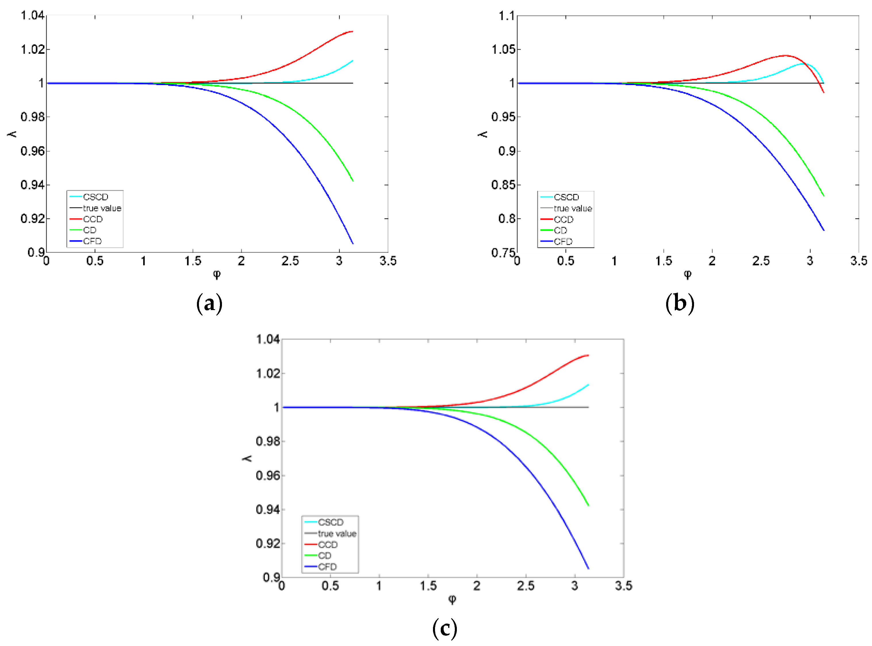
Ideally, if there is no numerical dispersion, then the velocity ratio $\lambda$ is equal to one. The larger the velocity ratio, the more serious the numerical dispersion. For comparison, we calculate the dispersion relation between velocity ratio and $kh$ for the central difference scheme (CFD), compact difference scheme (CD), CCD, and CSCD difference scheme. Figure 1 shows the velocity ratio curve for different $\theta$ for the above four methods in the isotropic ($\gamma =0$) condition.

Figure 1a–c show the velocity ratio curves for the CCD and CSCD schemes and the other two difference schemes using different $\theta$. The Courant numbers ($\alpha =v\Delta t/h$) are 0.25, the horizontal axis $\phi \in [0,\pi ]$ is the product of the wavenumber and the spatial step, and the vertical axis is the velocity ratio. A velocity ratio of one indicates that the numerical wave velocity is the same as the theoretical wave velocity, which shows that the method can suppress numerical dispersion better; otherwise, it indicates that the numerical dispersion of the method is worse. It can be seen that the dispersion phenomenon of the four methods is gradually intensified with the decrease in the number of spatial sampling points. The numerical dispersion of CSCD, CCD, and CD schemes is smaller than that of the CFD scheme, as their dispersion curves are closer to one. CSCD shows the best dispersion suppression, followed by CCD.

3.3. The Numerical Simulation Accuracy Analysis

To compare the numerical simulation accuracy of the models, we calculate the simulation error by simulating the two-dimensional plane harmonic initial value problem and then compare the numerical simulation accuracy of the CCD, CSCD, and CFD schemes. The initial value problem of the two-dimensional plane wave can be expressed as

$$\{\begin{array}{c}\frac{{\partial }^2{p}_{sh}\left(t,x,z\right)}{\partial t^2}=v^2\frac{{\partial }^2{p}_{sh}\left(t,x,z\right)}{\partial x^2}+v^2\frac{{\partial }^2{p}_{sh}\left(t,x,z\right)}{\partial z^2}\\ p_{sh}\left(0,x,z\right)=\cos \left(-\frac{2\pi f_0}{v}·\cos \theta ·x-\frac{2\pi f_0}{v}·\sin \theta ·z\right)\\ \frac{\partial p_{sh}\left(0,x,z\right)}{\partial t}=-2\pi f_0\sin \left(-\frac{2\pi f_0}{v}·\cos \theta ·x-\frac{2\pi f_0}{v}·\sin \theta ·z\right)\end{array}$$

(23)

where $v$ is the plane wave velocity, $\theta$ is the angle between the propagation direction and the x-axis, and $f_0$ is the frequency of the simple harmonic plane wave.

The analytical solution for the above initial value problem is

$$p_{sh}\left(t,x,z\right)=\cos \left[2\pi f_0\left(t-\frac{x}{v/\cos \theta }-\frac{z}{v/\sin \theta }\right)\right].$$

(24)

To simulate the two-dimensional shear wavefield, we specify the following: $f_0=20 \mathrm{Hz}$ and $\theta =\pi /4$, the wave velocity used is 1000 m/s, the length and depth of the model are 2000 m, the length of the vertical and horizontal grids are the same, and the sampling time is 1 s. The relative error of numerical simulation is calculated under different spatial mesh lengths and time steps, and it is defined as

$$E_r(\%)={\left\{\frac{1}{{\displaystyle \sum _{i=1}^N}{\displaystyle \sum _{j=1}^N}{\left[p_{sh}\left(t_n,x_i,z_j\right)\right]}^2}\sum _{i=1}^N\sum _{j=1}^N{\left[p_{sh}{}_{(i,j)}^n-p_{sh}\left(t_n,x_i,z_j\right)\right]}^2\right\}}^{\frac{1}{2}}\times 100$$

(25)

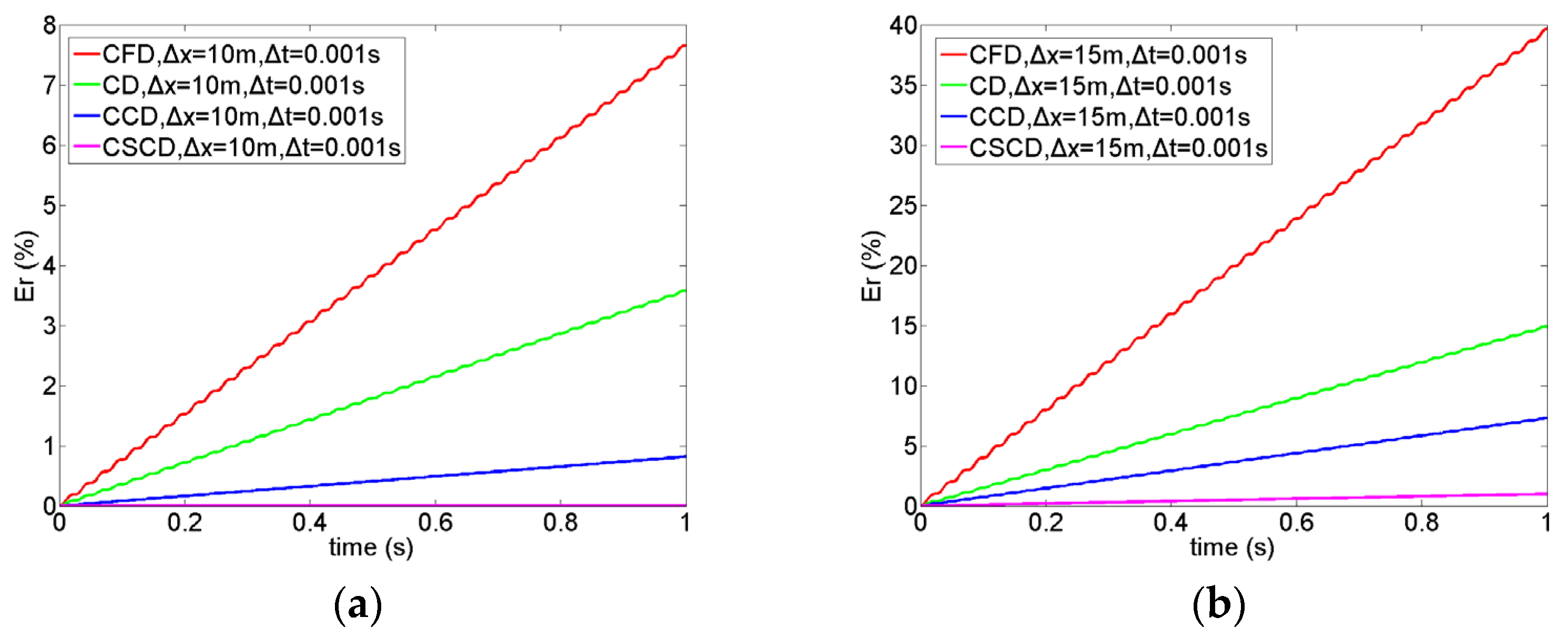
where $p_{sh}{}_{(i,j)}^n$ is the numerical solution, and $p_{sh}\left(t_n,x_i,z_j\right)$ is an analytical solution. We then compare the relative error curves of the CCD, CSCD, CD, and CFD schemes under different spatial steps (10 m, 15 m) and fixed time steps of 1 ms (Δt = 0.001 s), as shown in Figure 2. It can be seen from Figure 2 that the relative error gradually increases with increasing spatial grid length, time step, and simulation time. When the spatial step is 15 m and the time step is 1 ms, the maximum relative error of the CCD scheme is 8%, which is much smaller when compared with the maximum relative error of the CFD scheme (39%). When the smaller spatial gird size (10 m) is adopted, the accuracy is significantly improved, and the relative error is only 0.8%. The shear-wave simulation result using the CCD scheme has high accuracy and can handle the numerical simulation of the seismic wavefield with long sampling times. The simulation accuracy of the CSCD scheme is even higher than the CCD scheme. For CSCD, when the spatial gird size is 15 m, and the time step size is 1 ms, the maximum relative error is only 0.05%, further reducing to 0.0036% when a small spatial step (10 m) is used.

3.4. Comparison of Spatial Dispersion Suppression Effect

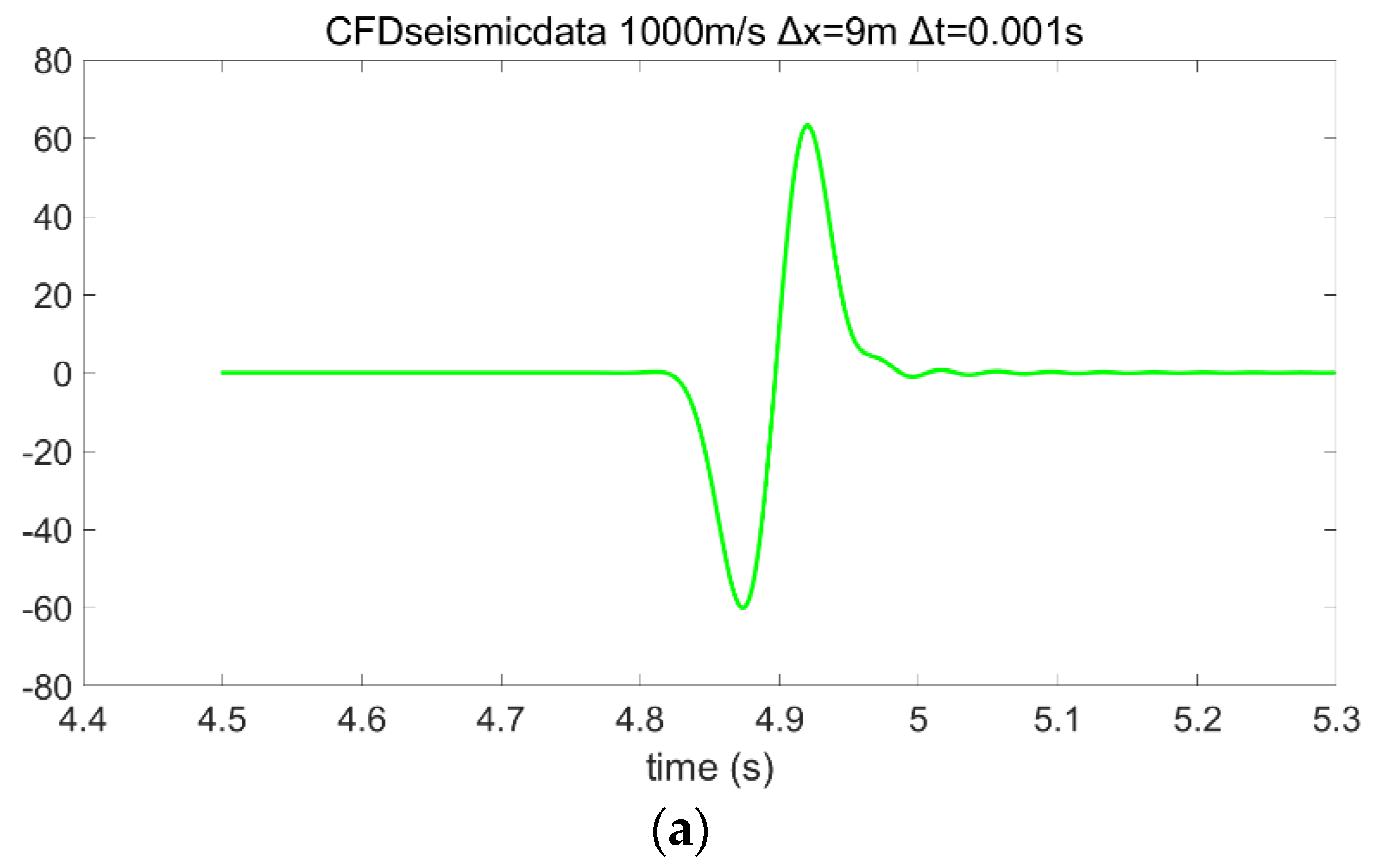
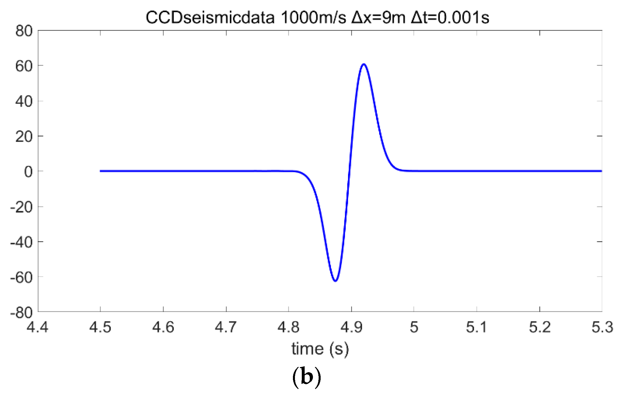
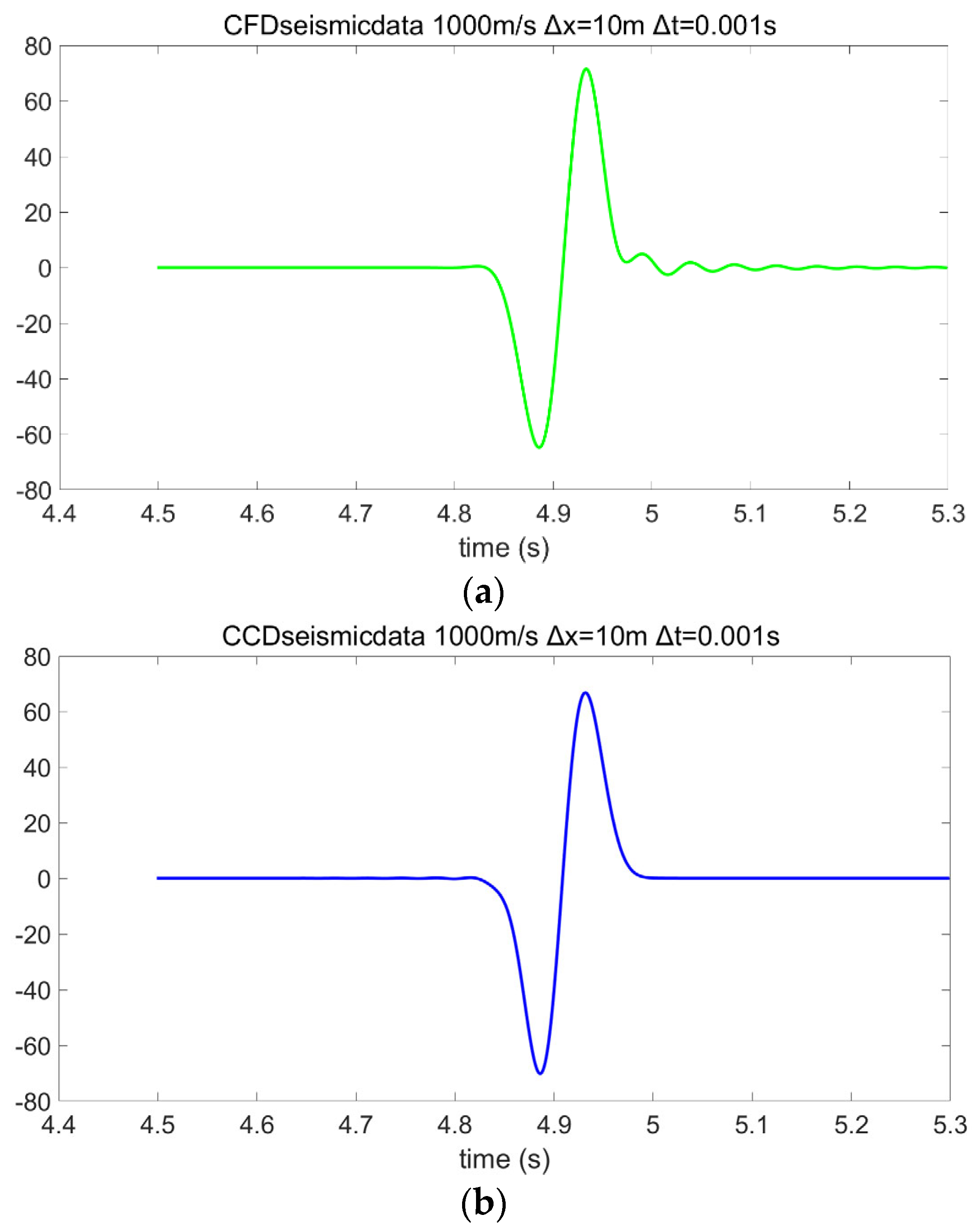
As the shear wave has the characteristics of low propagation speed, a one-dimensional low-speed homogeneous medium is constructed below. The velocity of the homogeneous medium model is 1000 m/s, the excitation position is located in the center of the model, and the source is a 10 Hz Rayleigh wavelet. Different space steps are set with a time step of 1 ms, the seismic records of 6 s are recorded, and the results are shown in Figure 3, Figure 4 and Figure 5. As shown in Figure 3, the traditional CFD scheme has numerical dispersion when the gird size is 9 m, and the dispersion increased substantially when the step increases to 10 m (Figure 5). In contrast, as shown in Figure 4, the corresponding seismic record calculated with the CCD scheme shows no numerical dispersion, and there is still no numerical dispersion when the gird size increases by 10 m (Figure 5).

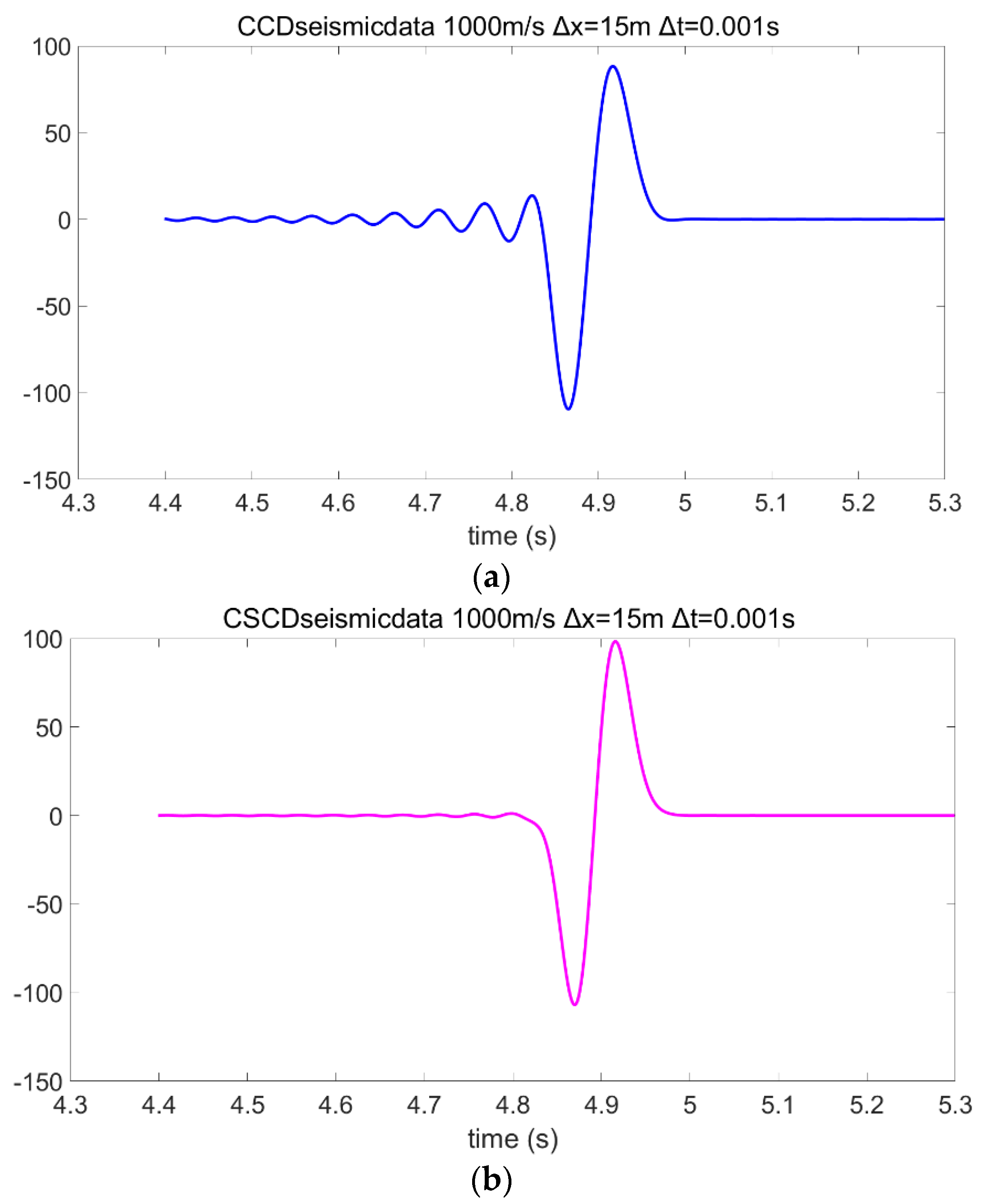
Figure 5a,b compare the numerical dispersion between the CCD and CSCD schemes when the step increases to 15 m. As shown in Figure 5a, at the speed of 1000 m/s, when the gird size continues to increase to 15 m, the CCD scheme shows dispersion, while the CSCD scheme shows no numerical dispersion at the same step. This confirms that the CSCD scheme improves the compactness of the CCD scheme and can better suppress the numerical dispersion so that a coarser grid may be used in the numerical simulation.

3.5. Time Dispersion Suppression Comparison

Seismic waves propagate in time and space. The numerical dispersion caused by grid discretization includes both spatial dispersion and time dispersion. The accuracy of time extrapolation of the traditional high-order difference (2 m, 2) scheme is only second order. When a large time step is adopted, there will be obvious time dispersion.

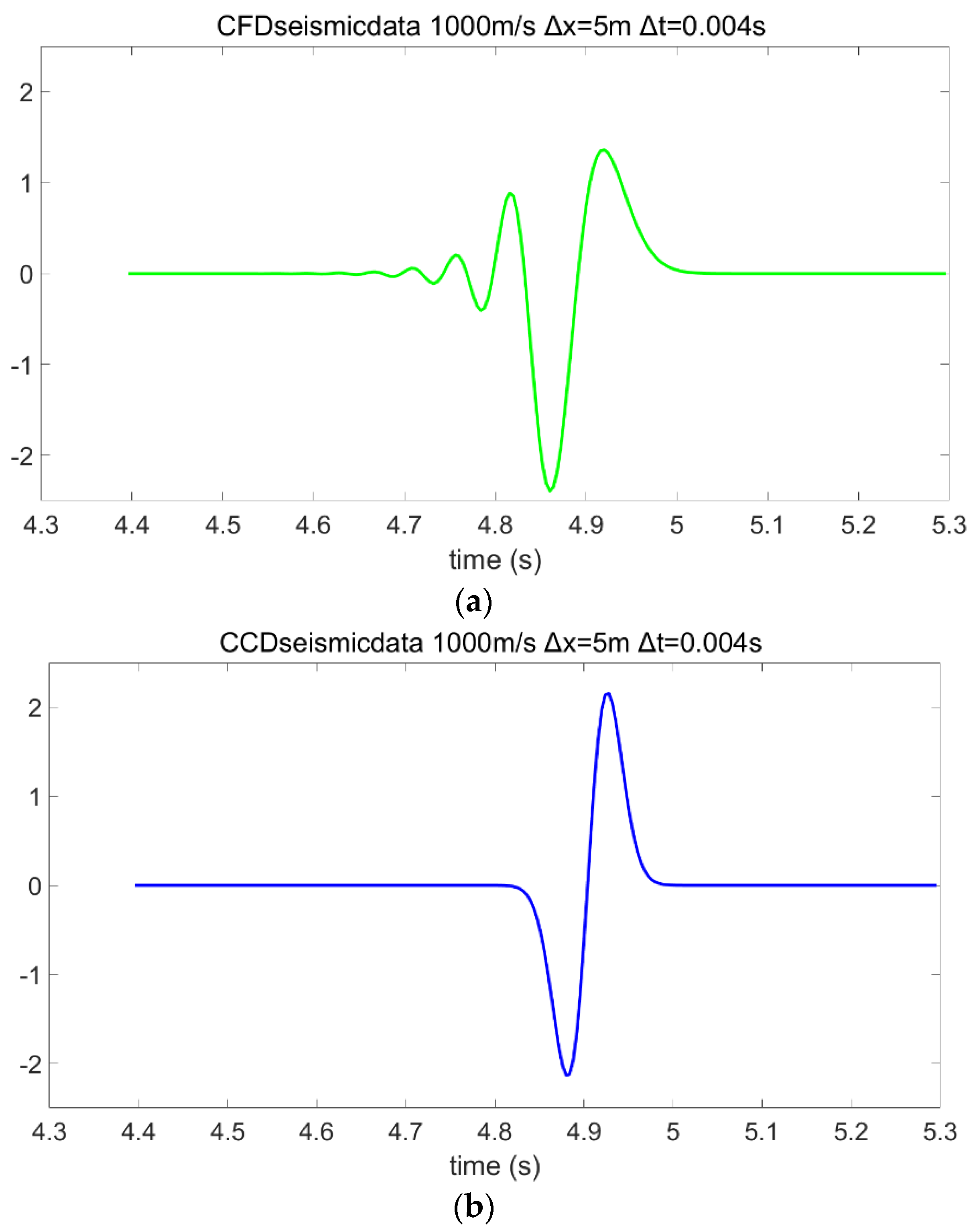
We use the same model to evaluate time dispersion as used for spatial dispersion. To evaluate time dispersion, it is necessary to eliminate the influence of numerical dispersion caused by the spatial gird size. Therefore, the spatial grid size is set to 5 m, and we increase the time step to 4 ms. The calculated seismic records of CCD and CFD are shown in Figure 6a,b.

The seismic record simulated using the CFD scheme shows serious and obvious dispersion, while the result of the CCD scheme shows almost no such dispersion. As the CCD scheme proposed in this paper uses the fourth-order difference operator to approximate the time partial derivative, it has better stability than the CFD scheme, which can only use the second-order difference operator to approximate the time partial derivative. The CSCD scheme, by contrast, uses the same fourth-order difference operator to approximate the time partial derivative, which shows even higher accuracy than the CCD scheme.

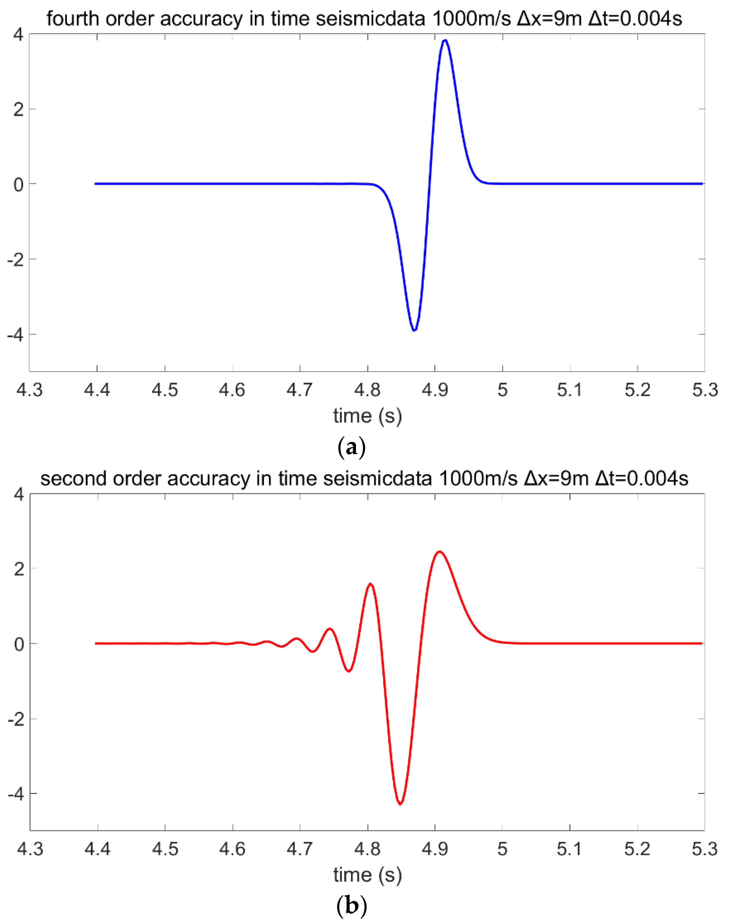
Figure 7a,b compare the seismic records using the fourth- and second-order difference operators to approximate the time partial derivative from the CCD scheme. It can be seen that when using the same finite difference scheme to suppress the numerical dispersion caused by the spatial gird size, the fourth-order operators show smaller numerical dispersion caused by increasing time step size than the second-order operators, which provides a theoretical basis for the use of large spatial gird size and large time step size for shear-wave simulation.

4. Shear-Wave (SH) RTM

4.1. Implementation of SH-RTM

The steps of shear-wave reverse-time migration, similar to those of traditional reverse-time migration, are as follows:

• Forward extrapolating of the source wavefield: starting from a given or estimated source wavefield, we solve the equation to forward propagate the source wavefield. Thus, for a source emitting at source positions $x_s,z_s$,

  $$V_y(x_s,z_s,t)=S(x_s,z_s,t)$$

  (26)
• Shear-wave reverse continuation: For receiver wavefield propagation, we reverse the R of the seismic receiver recorded in time and then set the initial receiver position as the initial boundary condition. We then use the selected finite difference scheme to solve the shear-wave equation (Equation (5)) iteratively to obtain the receiver wavefield. As shown in the following equation, where $x_r,z_r$ is the position of the source transmitter and receiver, and $T$ is the total duration of forward propagation.

  $$V_y(x_r,z_r,t)=R(x_r,z_r,T-t).$$

  (27)
• Imaging conditions of shear-wave application: the last step is to use the cross-correlation of source wavefield and receiver wavefield obtained in the previous two steps to obtain the image of the underground structure.

  $$I(x,z)={\displaystyle {\int }_0^{T}S(x,z,t)R(x,z,t)}dt.$$

  (28)

4.2. Shear-Wave Reverse-Time Migration in Marmousi Models

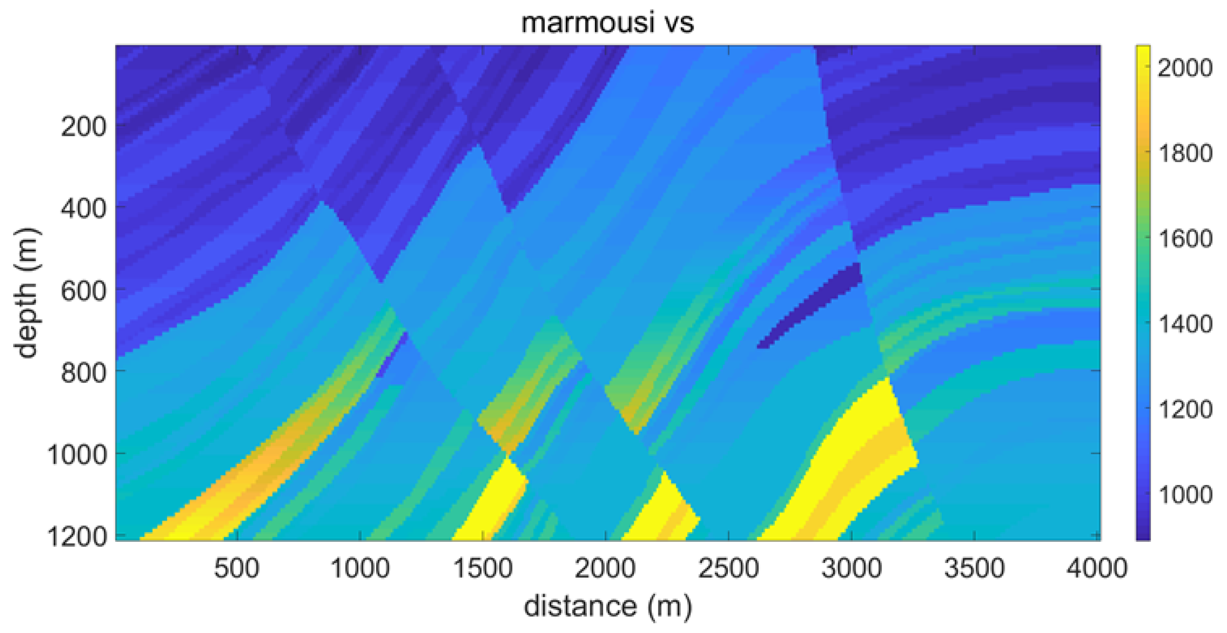
A set of two-dimensional Marmousi models are set up, as shown in Figure 8 and Figure 9, where the S-wave velocity (Figure 9) is modified by the ratio of horizontal to vertical P-wave velocity (Figure 8). The model size is 121 × 401 grid points, the spatial grid size Δx = 10 m, the time step is 1 ms, the Ricker wavelet of 20 Hz is excited, and the sampling time is 4 s. With these initial conditions, the reverse-time migration imaging is then carried out.

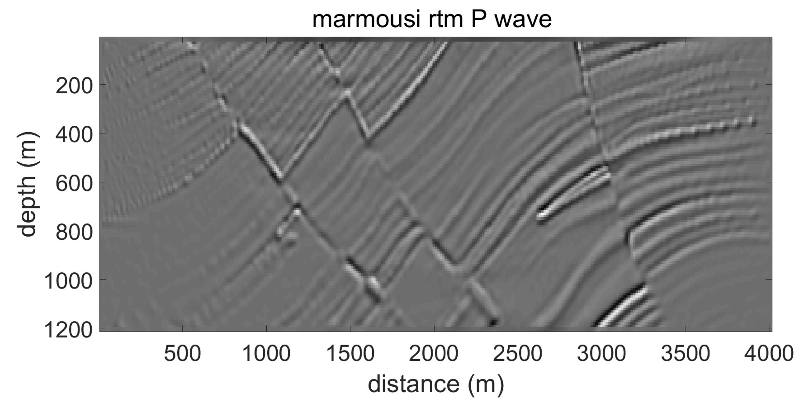
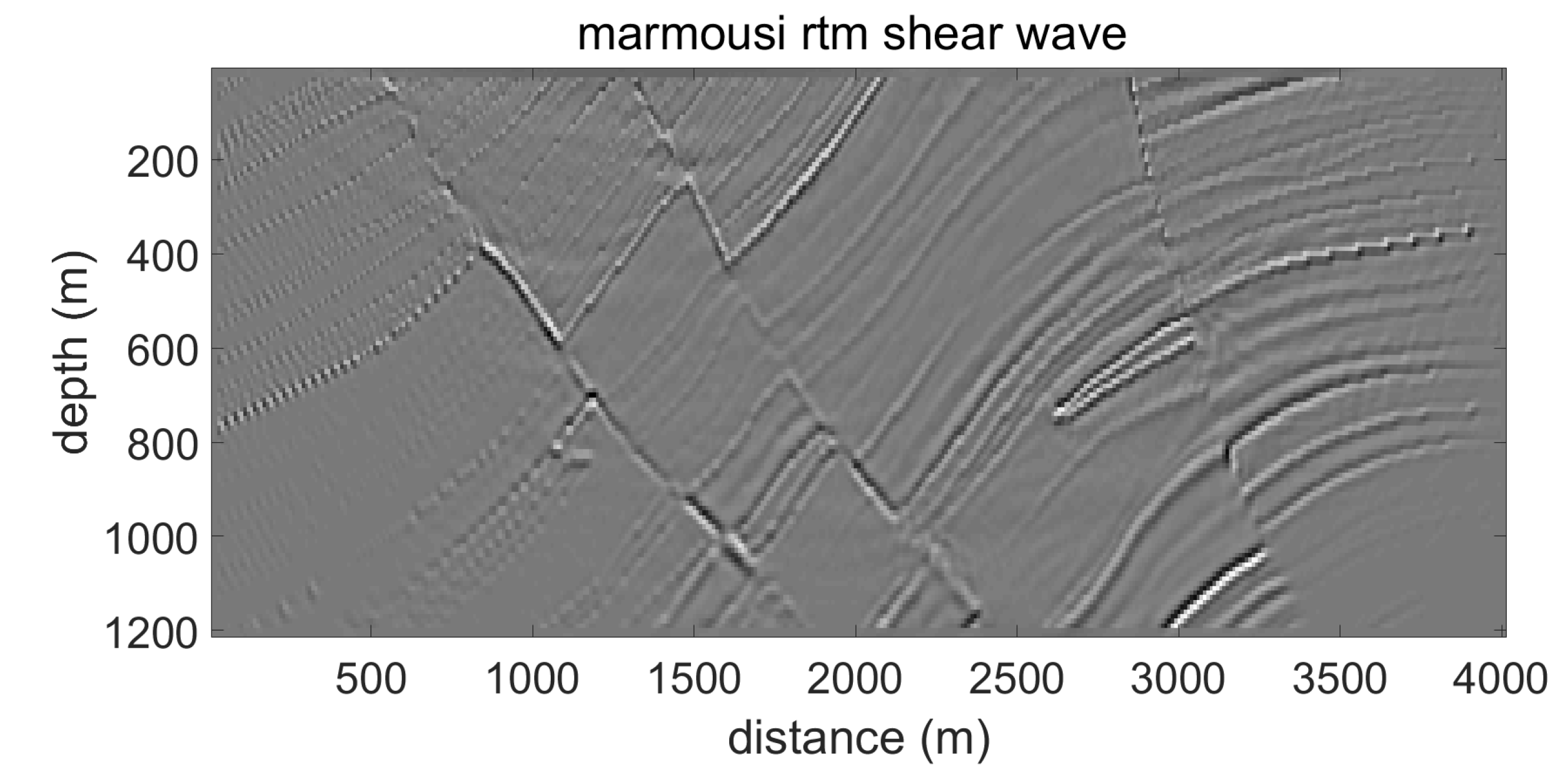
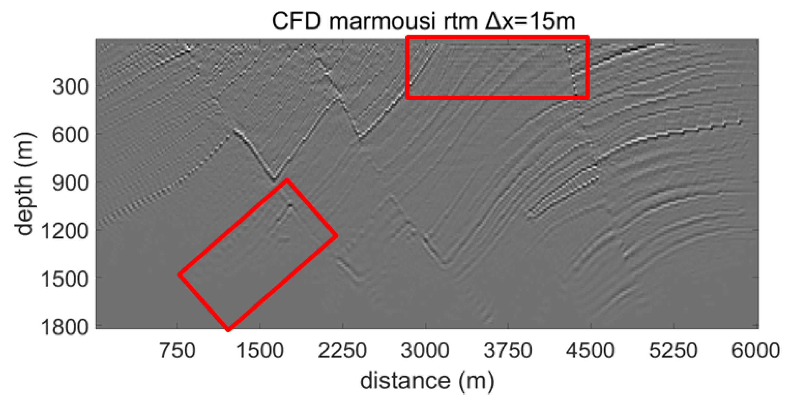
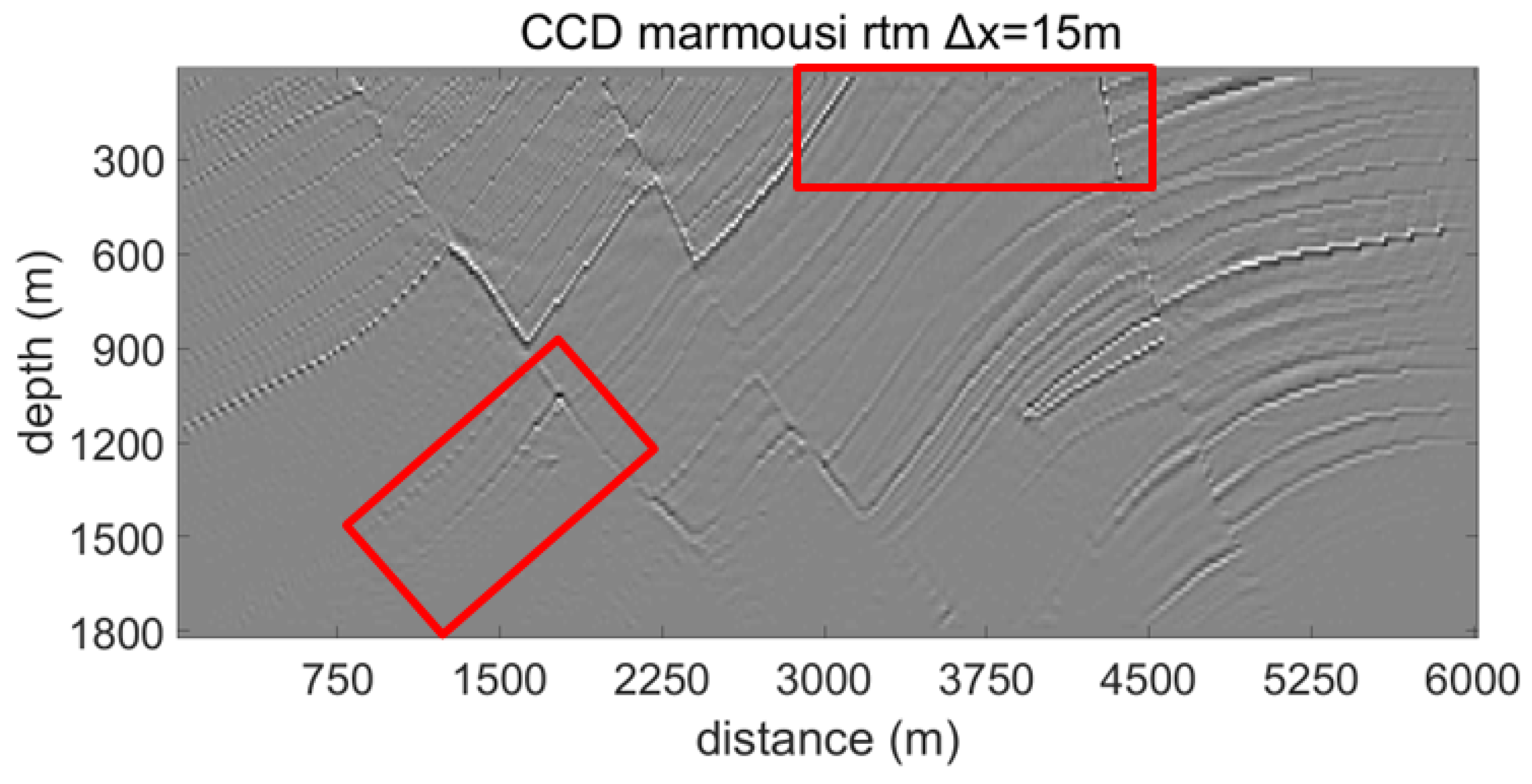
We use the acoustic-wave equation and P-wave source loading method for the reverse-time migration of the P-wave velocity (Figure 10), and the shear-wave equation and shear-wave source loading method for the reverse-time migration of the S-wave velocity (Figure 11). The result of using shear-wave velocity for reverse-time migration (Figure 11) has clearer structural definitions and higher resolution compared with the result of acoustic reverse-time migration using P-wave velocity in Figure 10. We then continue with the SH reverse-time migration imaging experiment, by increasing the spatial gird size, setting Δx = 15 m, get new S-wave velocity Marmousi model (Figure 12) and the sampling time to 4000 ms. The images for different differential methods are then compared. The following figures (Figure 13, Figure 14 and Figure 15) show the reverse-time migration results of the Marmousi model in the shear-wave equation using different finite difference schemes.

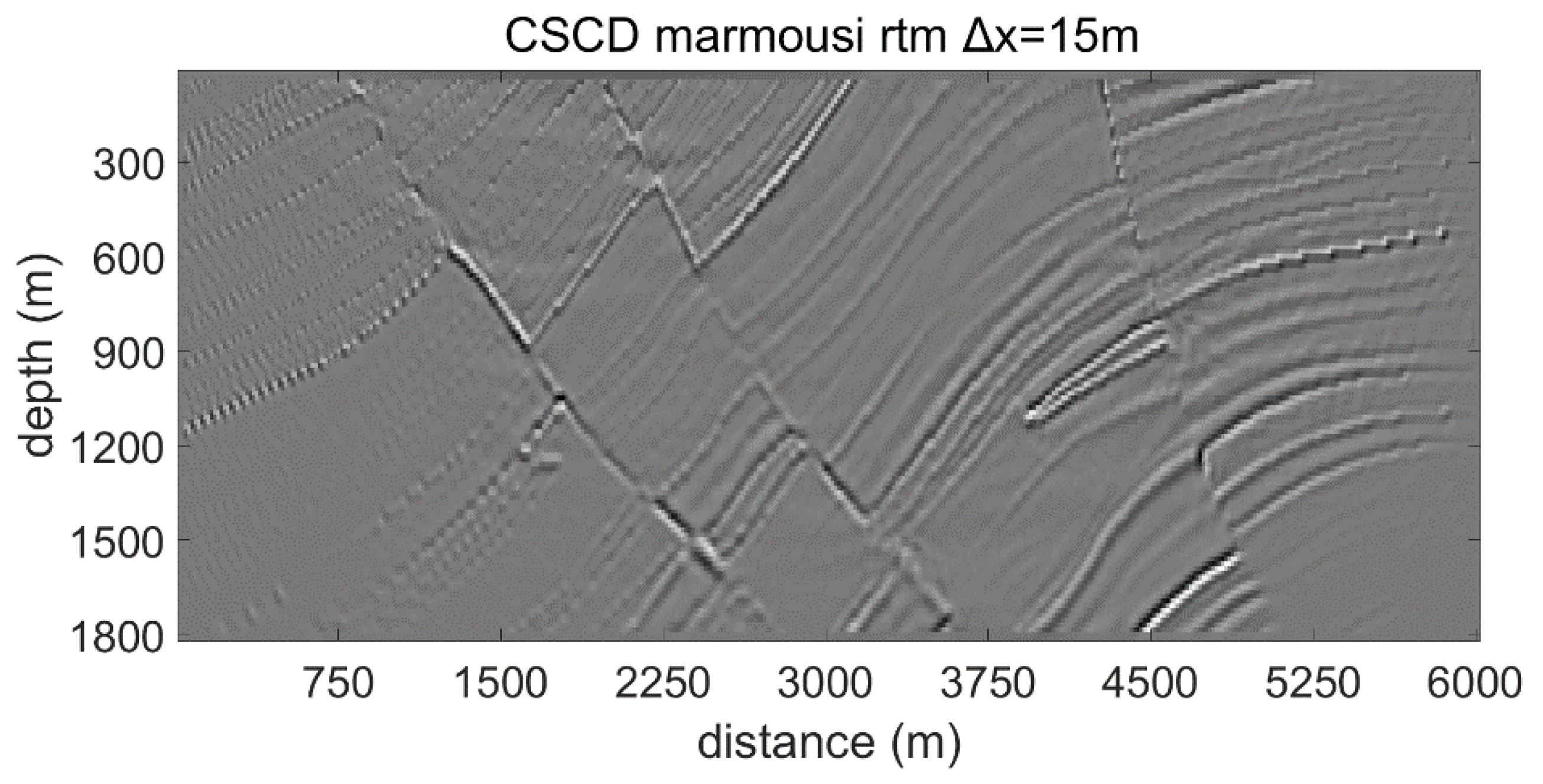
As shown in Figure 13 and Figure 14, the CCD scheme yields better imaging than the CFD scheme, where the red boxes mark the area of improvement, due to higher accuracy in accounting for numerical dispersion caused by the spatial gird size. Compared with Figure 13 and Figure 14, the CSCD scheme produces the best imaging results of the Marmousi model (Figure 15).

5. Conclusions

In this paper, we proposed a fourth-order time difference solution for the shear-wave equation using the supercompact difference scheme and the combined supercompact difference scheme. We carried out a detailed comparison of their accuracy in numerical simulations and reverse-time migrations. Thus, we reached the following conclusions:

The combined compact difference scheme (CCD) has the characteristics of low numerical dispersion, high stability, and simulation accuracy. It is suitable for the numerical simulation of the seismic wavefield with large space and time steps. It provides an effective method for simulating shear-wave propagation and implementing shear-wave reverse-time migration.

The combined supercompact difference scheme (CSCD) is extended and optimized from the combined compact difference scheme (CCD). Compared with its prototype, the supercompact difference scheme, the combined supercompact difference scheme further suppresses the numerical dispersion caused by the increase in spatial step length and is suitable for numerical simulation with even larger spatial step length.

Finally, we carried out the reverse-time migration imaging of the Marmousi model of shear-wave velocity under isotropic conditions. The combined supercompact difference scheme (CSCD) yields the best shear-wave imaging results of the Marmousi model when compared with the other methods. These results reveal the potential for further extending the supercompact difference scheme and the combined supercompact difference scheme forward simulation of shear waves in complex media such as two-dimensional or three-dimensional anisotropic media and viscoelastic media. It is worth highlighting that the method presented in this paper is restricted to isotropic media at the moment. However, these results reveal the potential for further extending the supercompact difference scheme and the combined supercompact difference scheme forward simulation of shear-wave in complex media such as two-dimensional or three-dimensional anisotropic or viscoelastic media. Of course, the method in this paper also has its limitations, such as low computational efficiency, making it very challenging to apply to three-dimensional media, which is also the focus of our subsequent research.

References

- Gray, S.H.; Etgen, J.; Dellinger, J.; Whitmore, D. Seismic migration problems and solutions. Geophysics 2001, 66, 1622–1640. [Google Scholar] [CrossRef]
- Yilmaz, O. Seismic data analysis. Soc. Expl. Geophys. 2001, 1230–1280. [Google Scholar]
- Leveille, J.P.; Jones, I.F.; Zhou, Z.Z.; Wang, B.; Liu, F. Subsalt imaging for exploration, production, and development: A review. Geophysics 2017, 76, WB3–WB20. [Google Scholar] [CrossRef]
- Liu, H.; Dai, N.; Niu, F.; Wu, W. An explicit time evolution method for acoustic wave propagation. Geophysics 2014, 79, T117–T124. [Google Scholar] [CrossRef] [Green Version]
- Huang, J.Q.; Li, Z.C.; Huang, J.P.; Zhang, J.; Sun, W. Lebedev grid high-order finite-difference modeling and elastic wave-mode separation for TTI media. Oil Geophys. Prospect. 2017, 52, 915–927. [Google Scholar]
- Amundsen, L.; Ørjan, P. Time step n-tupling for wave equations. Geophysics 2017, 82, T249–T254. [Google Scholar] [CrossRef]
- Chu, C.L.; Stoffa, P.L. An implicit finite-difference operator for the Helmholtz equation. Geophysics 2012, 77, T97–T107. [Google Scholar] [CrossRef]
- Jiang, Z.D.; Fan, C.W.; Li, X.Z.; Deng, G.J.; Chen, K.; Li, Y.S. Numerical simulation of marine ghost wave based on high order finite difference method with variable grids. Prog. Geophys. 2021, 36, 365–373. [Google Scholar] [CrossRef]
- Li, B.; Liu, Y.; Sen, M.K.; Ren, Z. Time-space-domain mesh-free finite difference based on least squares for 2D acoustic-wave modeling. Geophysics 2017, 82, T143–T157. [Google Scholar] [CrossRef]
- Liu, L.B.; Duan, P.R.; Zhang, Y.Y.; Tian, K.; Tan, M.Y.; Li, Z.C.; Dou, J.Y.; Li, Q.Y. Overview of mesh-free method of seismic forward numerical simulation. Prog. Geophys. 2020, 35, 1815–1825. [Google Scholar] [CrossRef]
- Wang, E.J.; Liu, Y.; Sen, M.K. Effective finite-difference modelling methods with 2-D acoustic wave equation using a combination of cross and rhombus stencils. Geophys. J. Int. 2016, 206, 1933–1958. [Google Scholar] [CrossRef]
- Zhang, B.Q.; Zhou, H.; Chen, H.M.; Shen, S.B. Time-space domain high-order finite difference method for seismic wave numerical simulation based on new stencils. Chin. J. Geophys. 2016, 59, 1804–1814. [Google Scholar] [CrossRef]
- Duan, Y.T.; Sava, P. Scalar imaging condition for elastic reverse time migration. Geophysics 2015, 80, S127–S136. [Google Scholar] [CrossRef] [Green Version]
- Adams, N.A.; Shariff, K.A. High-resolution hybrid compact-ENO scheme for Shock-Turbulence interaction problems. J. Comput. Phys. 1996, 127, 27–51. [Google Scholar] [CrossRef]
- Dennis, S.C.R.; Hundson, J.D. Compact h4 finite-difference approximations to operators of Navier-Stokes type. J. Comput. Phys. 1989, 85, 390–416. [Google Scholar] [CrossRef]
- Lele, S.K. Compact finite difference scheme with spectral-like resolution. J. Comput. Phys. 1992, 103, 16–42. [Google Scholar] [CrossRef]
- Chu, P.C.; Fan, C.W. A three-point combined compact difference scheme. J. Comput. Phys. 1998, 140, 370–399. [Google Scholar] [CrossRef] [Green Version]
- Chang, W.; McMechan, G.A. 3-D elastic prestack, reverse-time depth migration. Geophysics 1994, 59, 597–609. [Google Scholar] [CrossRef]
- Du, Q.Z.; Zhu, Y.T.; Ba, J. Polarity reversal correction for elastic reverse time migration. Geophysics 2012, 77, S31–S41. [Google Scholar] [CrossRef]
- Dai, N.; Wu, W.; Zhang, W.; Wu, X. TTI RTM using variable grid in depth. In Proceedings of the International Petroleum Technology Conference, Bangkok, Thailand, 7–9 February 2012; pp. 1–7. [Google Scholar]
- Zhang, J.; Tian, Z.; Wang, C. P- and S-wave separated elastic wave equation numerical modeling using 2D staggered-grid. In Proceedings of the 77th Annual International Meeting, SEG, San Antonio, TX, USA, 14 September 2007; pp. 2104–2109. [Google Scholar]
- Xiao, X.; Leaney, W.S. Local vertical seismic profiling (VSP)elastic reverse-time migration and migration resolution: Salt-flank imaging with transmitted P-to-S waves. Geophysics 2010, 75, S35–S49. [Google Scholar] [CrossRef]
- Gu, B.; Li, Z.; Ma, X.; Liang, G. Multi-component elastic reverse time migration based on the P and S separating elastic velocity-stress equation. J. Appl. Geophys. 2015, 112C, 62–78. [Google Scholar] [CrossRef]
- Wang, W.; McMechan, G.A.; Zhang, Q. Comparison of two algorithms for isotropic elastic P and S decomposition in the vector domain. Geophysics 2015, 80, T147–T160. [Google Scholar] [CrossRef] [Green Version]
- Du, Q.; Gong, X.; Zhang, M.; Zhu, Y.; Fang, G. 3D PS-wave imaging with elastic reverse-time migration. Geophysics 2014, 79, S173–S184. [Google Scholar] [CrossRef]
- Zhang, Q.; McMechan, G.A. 2D and 3D elastic wavefield vector decomposition in the wavenumber domain for VTI media. Geophysics 2010, 75, D13–D26. [Google Scholar] [CrossRef]
- Du, Q.Z.; Guo, C.F.; Zhao, Q.; Gong, X.; Wang, C.; Li, X.Y. Vector-based elastic reverse time migration based on scalar imaging condition. Geophysics 2017, 82, S111–S127. [Google Scholar] [CrossRef]
- Nguyen, B.D.; McMechan, G.A. Five ways to avoid storing source wavefield snapshots in 2D elastic prestack reverse time migration. Geophysics 2015, 80, S1–S18. [Google Scholar] [CrossRef]
- Li, X.; Zhang, S. Forty years of shear-wave splitting in seismic exploration: An overview. Geophys. Prospect. Pet. 2021, 60, 190–209. [Google Scholar]
- Bouchaala, F.; Ali, M.Y.; Matsushima, J. Compressional and shear wave attenuations from walkway VSP and sonic data in an offshore Abu Dhabi oilfield. Comptes Rendus Géosci. 2021, 353, 337–354. [Google Scholar] [CrossRef]
- Wu, Y.; He, Z.; Hu, J.; Deng, Z.; Wang, Y.; Yin, W. P-wave and S-wave Joint Acquisition Technology and Its Application in Sanhu Area. In Proceedings of the 88th Annual International Meeting, Anaheim, CA, USA, 14 October 2018; pp. 1–5. [Google Scholar]
- Wang, S.Q.; Yang, D.H.; Yang, K.D. Compact finite difference scheme for elastic equations. J. Tsinghua Univ. 2002, 42, 1128–1131. [Google Scholar]
- Bouchaala, F.; Guennou, C. Estimation of viscoelastic attenuation of real seismic data by use of ray tracing software: Application to the detection of gas hydrates and free gas. Comptes Rendus Géosci. 2012, 344, 57–66. [Google Scholar] [CrossRef]
- Zhu, T.; Harris, J.M.; Biondi, B. Q-compensated reverse-time migration. Geophysics 2014, 79, S77–S87. [Google Scholar] [CrossRef] [Green Version]
- Liu, F.; Zhang, G.; Morton, S.A.; Leveille, J.P. An effective imaging condition for reverse-time migration using wavefield decomposition. Geophysics 2011, 76, S29–S39. [Google Scholar] [CrossRef]
- Moradpouri, F.; Moradzadeh, A.; Pestana, R.N.C.; Ghaedrahmati, R.; Soleimani, M. An improvement in wave-field extrapolation and imaging condition to suppress RTM artifacts. Geophysics 2017, 82, S403–S409. [Google Scholar] [CrossRef]
- Moradpouri, F.; Morad-Zadeh, A.; Pestana, R.C.; Soleimani, M. Seismic reverse time migration using a new wave field extrapolator and a new imaging condition. Acta Geophys. 2016, 64, 1673–1690. [Google Scholar] [CrossRef] [Green Version]
- Virieux, J. SH-wave propagation in heterogeneous media: Velocity-stress finite-difference method. Geophysics 1984, 49, 1933–1942. [Google Scholar] [CrossRef]
- Wang, Y.; Shi, H.G.; Zhou, C.Y.; Gui, Z.X. Numerical simulation of 2D seismic wave-field used combined compact difference scheme. Chin. J. Geophys. 2018, 61, 4568–4583. [Google Scholar]
- Dong, L.; Zhan, J. Combined super compact finite difference scheme and application to simulation of shallow water equations. Chin. J. Comput. Mech. 2008, 25, 791–796. [Google Scholar]
- Blayo, E. Compact finite difference schemes for ocean models. J. Comput. Phys. 2000, 164, 241–257. [Google Scholar] [CrossRef]
- Sengupta, T.K.; Ganeriwal, G.; De, S. Analysis of central and upwind compact schemes. J. Comput. Phys. 2003, 192, 677–694. [Google Scholar] [CrossRef]
- Wu, G.C.; Wang, H.Z. Analysis of numerical dispersion in wave2field simulation. Prog. Geophys. 2005, 20, 58–65. [Google Scholar]
Figure 1.
Velocity ratio curves for different numerical simulation methods. The blue curve is the traditional central difference scheme, the green curve is the traditional implicit difference scheme, the red curve is the CCD difference scheme, the blue curve is the CSCD difference scheme, and the black line is the velocity ratio constant of 1: (a) ; (b) ; (c) .
Figure 2.
Relative errors of numerical simulation for different schemes and gird size: (a) Δx = 10 m, Δt = 0.001 s; (b) Δx = 15 m, Δt = 0.001 s.
Figure 3.
(a) CFD is used to simulate the numerical simulation of seismic records in the 1D homogeneous medium model, Δx = 9 m; (b) CCD is used to simulate the numerical simulation of seismic records in the 1D homogeneous medium model, Δx = 9 m.
Figure 4.
(a) CFD is used to simulate the numerical simulation of seismic records in the 1D homogeneous medium model, Δx = 10 m; (b) CCD is used to simulate the numerical simulation of seismic records in the 1D homogeneous medium model, Δx = 10 m.
Figure 5.
(a) CCD is used to simulate the numerical simulation of seismic records in the 1D homogeneous medium model, Δx = 15 m; (b) CSCD is used to simulate the numerical simulation of seismic records in the 1D homogeneous medium model, Δx = 15 m.
Figure 6.
(a) CFD is used to simulate the numerical simulation of seismic records in the 1D homogeneous medium model, Δt = 0.004 s; (b) CCD is used to simulate the numerical simulation of seismic records in the 1D homogeneous medium model, Δt = 0.004 s.
Figure 7.
(a) CCD is used to simulate the numerical simulation of seismic records in the 1D homogeneous medium model with fourth-order accuracy in time, dt = 0.004 s; (b) CCD is used to simulate the numerical simulation of seismic records in the 1D homogeneous medium model with second-order accuracy in time, dt = 0.004 s.
Figure 8.
Marmousi model: acoustic velocity model.
Figure 9.
Marmousi model: shear-wave velocity model.
Figure 10.
The reverse-time migration result with Marmousi acoustic velocity model.
Figure 11.
The reverse-time migration result with Marmousi shear-wave velocity model.
Figure 12.
Figure 13.
CFD is used for the reverse-time migration result with Marmousi shear-wave velocity model, Δx = 15 m.
Figure 14.
CCD is used to the reverse-time migration result with Marmousi shear-wave velocity model, Δx = 15 m.
Figure 15.
CSCD is used for the reverse-time migration result with Marmousi shear-wave velocity model, Δx = 15 m.