
Seismic Velocity Anomalies Detection Based on a Modified U-Net Framework

1
School of Mathematics, Jilin University, Changchun 130012, China
2
National Applied Mathematical Center (Jilin), Changchun 130012, China
3
College of Geoexploration Science and Technology, Jilin University, Changchun 130061, China
*
Author to whom correspondence should be addressed.
Appl. Sci. 2022, 12(14), 7225; https://0-doi-org.brum.beds.ac.uk/10.3390/app12147225
Submission received: 9 June 2022
/
Revised: 12 July 2022
/
Accepted: 13 July 2022
/
Published: 18 July 2022
(This article belongs to the Special Issue Technological Advances in Seismic Data Processing and Imaging)
Abstract
:Accurate and efficient reconstruction of hidden geological structures under the surface is the main task of high-resolution Velocity Model Building (VMB). The most commonly used methods in practice are Tomography and Full Waveform Inversion (FWI), which rely heavily on the initial model. Recently, deep learning types of methods have received widespread attention and have performed well in many tasks such as image segmentation and classification. Therefore, it is of great significance to introduce deep learning algorithms into the VMB procedure to accelerate the production cycle, especially for the velocity anomalies detection, which is crucial for a high-resolution initial model. In this paper, a modified U-Net framework is proposed and applied directly on the seismic shot gathers to identify anomalies in the early stage of VMB, which can provide a suitable initial guess for the following large-scale VMB procedures such as FWI. The numerical examples show the power of the proposed method on synthetic data.
1. Introduction
The main goal of the high-resolution Velocity Model Building process is to reconstruct the subsurface structures, especially to capture potential geological bodies, such as shallow gas clouds, salt bodies and fault plains. On the other hand, these complex geological structures result in certain types of anomalies. Refs. [1,2] proposed different methods to calculate velocity models. Particularly, gas clouds correspond to lower velocity and a smaller Quality Factor (Q) [3], and some quantifiable techniques were proposed to identify shallow gas pockets. A ray-based Q-tomography was developed by [4] and has been applied to field data to estimate the effects of shallow gas by representing the pockets as anomalous Q bodies [5]. One of the most crucial problems in the Q-tomography method is how to predict the Q bodies masks accurately, which is used to indicate the location of strong absorptions. Usually, several iterations were needed to improve the precision of the location information, either by manual editing or introducing some attributes as pilot. Refs. [6,7] show exciting Q-tomography results, employing the FWI model to produce the masks for the subsequent anomalous Q-tomography process to evaluate the shallow gas clouds. However, in the FWI guided Q-tomography flow, the accuracy of the masks is strongly dependent on the FWI process, human intervention, and the initial Q-factor model, which are extremely time-consuming and tedious. The initial Q-factor model can be directly obtained from field data by applying sophisticated methods [8]. Furthermore, the initial velocity model usually starts from a smooth one, which is based on manual velocity analysis or vintage experience from that area only; the local detailed information is excluded. Introducing accurate location information into velocity models automatically in the early stages will help to improve the quality of the VMB results and accelerate the model building process significantly.
Since deep learning was proposed by [9], it has received widespread attention and is widely used in computer vision, voice recognition, natural language processing, etc. Recently, machine-learning based techniques were introduced into the seismic data processing and interpretation community. Ref. [10] presented a supervised-learning-based salt body detection algorithm. Three features—amplitude, second derivative and curve length—were selected to characterize voxels of 3D seismic volume, and the algorithm uses small fraction of the characterized voxels for training to predict the whole volume. Ref. [11] developed a texture classification workflow using seismic attributes, clustering techniques and segmentation by thresholds, followed by second step mathematical morphological and basic operations between volumes to improve the detection. A major strategy of this type of method is to apply data mining algorithms [12] on the post-migration volumes. Ref. [13] developed a novel method based on machine learning techniques to automatically identify and localize faults. The method was introduced in the initial stages of the VMB process, when no seismic data had been migrated, which is different from other types of post-migration methods that use processed seismic data or migrated images [14,15].
In the field of computer vision, it is well known that Fully Convolutional Networks (FCNs) and U-Net perform well on image segmentation tasks. These two frameworks were proposed by [16,17], respectively. U-Net is similar to FCN and has been widely used in medical image segmentation. Compared with FCN, the first feature of U-Net is that it is completely symmetrical, which means the left and right hand side are very similar. However, the decoder of FCN is relatively simple, using only a deconvolution operation. The second difference is skip connection: FCN uses summation, while U-Net uses concatenation. The U-Net model modified and expanded the network on the basis of FCN, so that it can use very few training images to obtain very accurate segmentation results. In addition, an upsampling stage is added, which adds lots of feature channels, allowing more texture information of the original image to spread in high-resolution layers. U-net does not have a fully convolutional layer and uses valid for convolution throughout, which ensures that the results of the segmentation are based on no missing context features.
In this paper, a two-step deep-learning based velocity anomalies detection workflow is established. The workflow starts from the pre-migration shot gathers directly, justifiying the presence of anomalies firstly and then predicting accurate location information of the velocity anomalies prior to VMB process by employing a modified U-Net neural network. A set of two-dimensional synthetic model tests are presented to evaluate the effectiveness of the proposed workflow.
2. Materials and Methods
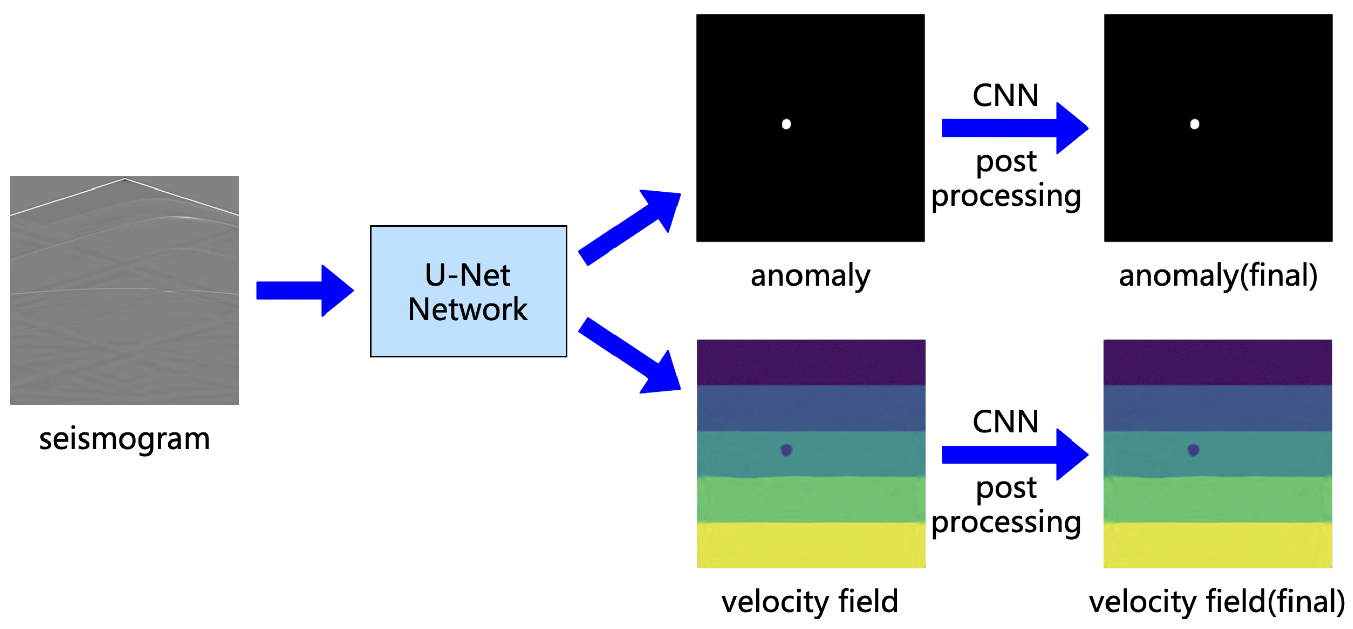
In this section, the flow chart of the proposed model is presented, including a 2-branch U-Net and a post-processing step.
2.1. Seismic Data Preparation
Firstly, a set of two-dimensional layered velocity models with anomalies are generated; the models include high or low speed anomaly regions. An acoustic wave equation forward modeling scheme is employed for producing seismic data based on the generated velocity models. The detailed settings are listed here.
- Background velocity can be simple layered model or including faults.
- Anomalies are simplified to some elliptical regions, with random center coordinates and major/minor axis length.
- Masks for the designed anomalies are generated simultaneously.
- At most, two anomalies are located in each model, either inside one layer or crossing multiple layers.
- Seismic data generated by different shots are recorded.
- All the data are separated into two parts for training and testing.
2.2. Flow Chart
The flow chart of the proposed framework is presented in Figure 1.
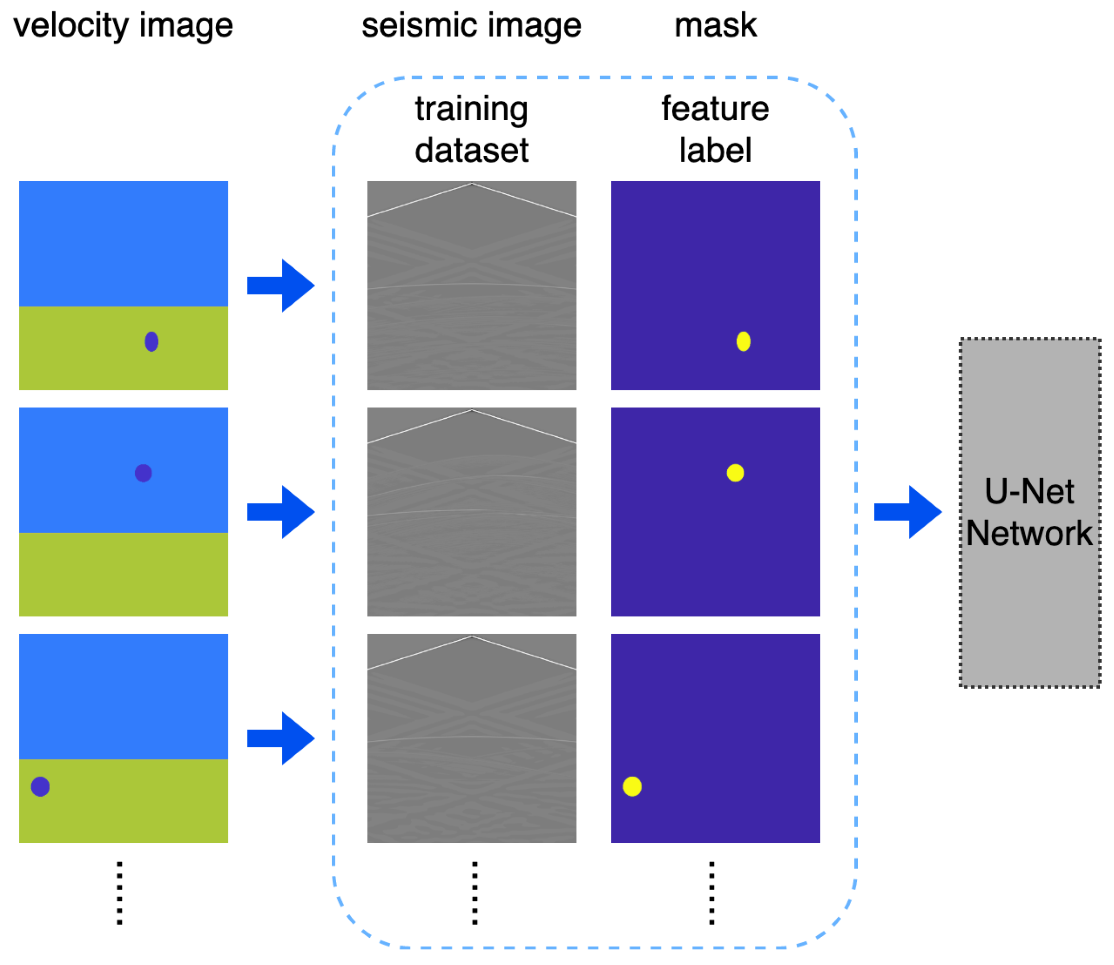
The pairs of generated seismic and the corresponding mask compose the training dataset and feature label, as the input for the proposed U-Net neural network. The training procedure is shown in Figure 2.
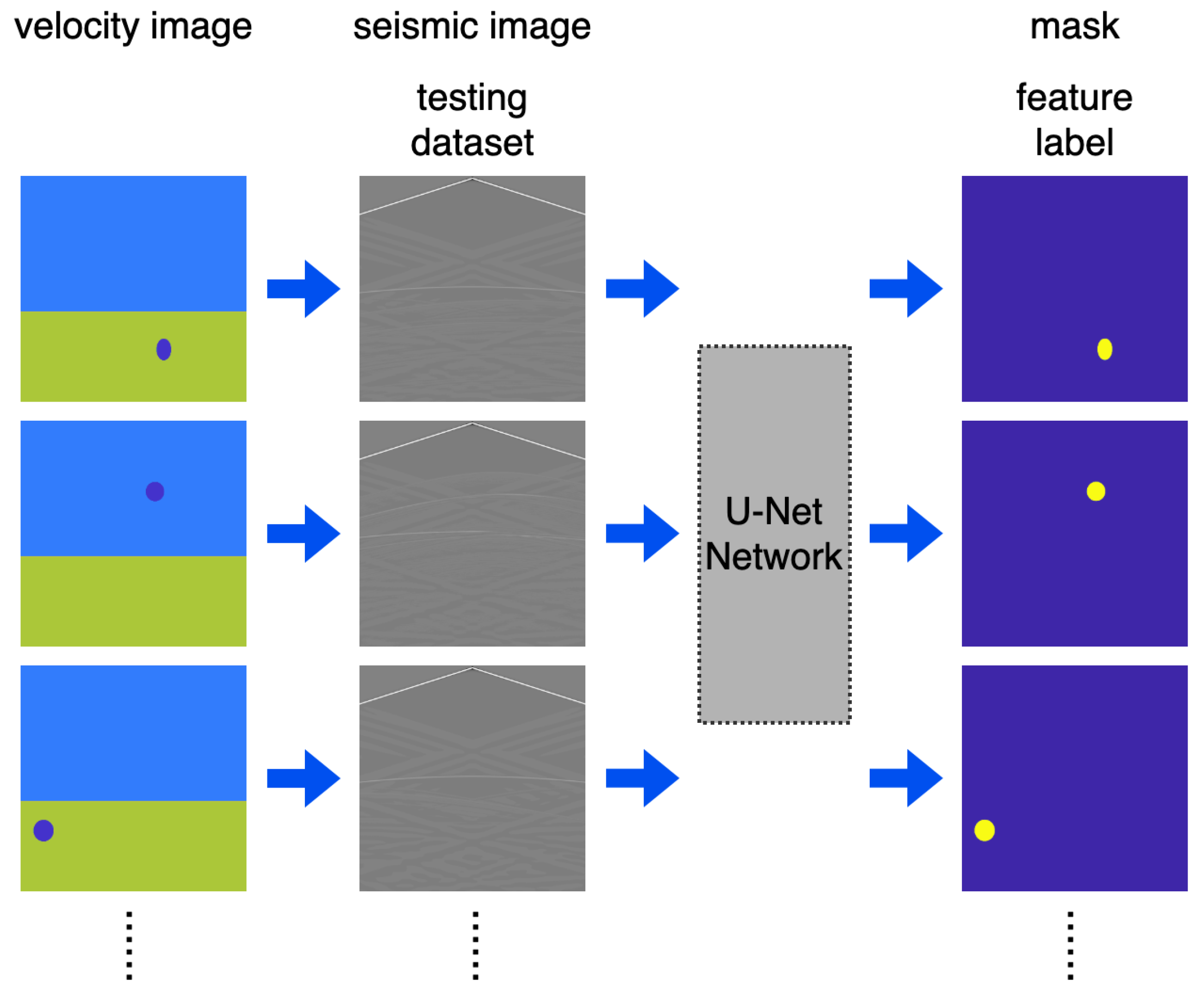
After the training process, the testing data (not included in training) will be input to the trained U-Net neural network, and the feature label set is predicted for verification purposes, which is shown in Figure 3.
2.3. Modified U-Net Neuron Network
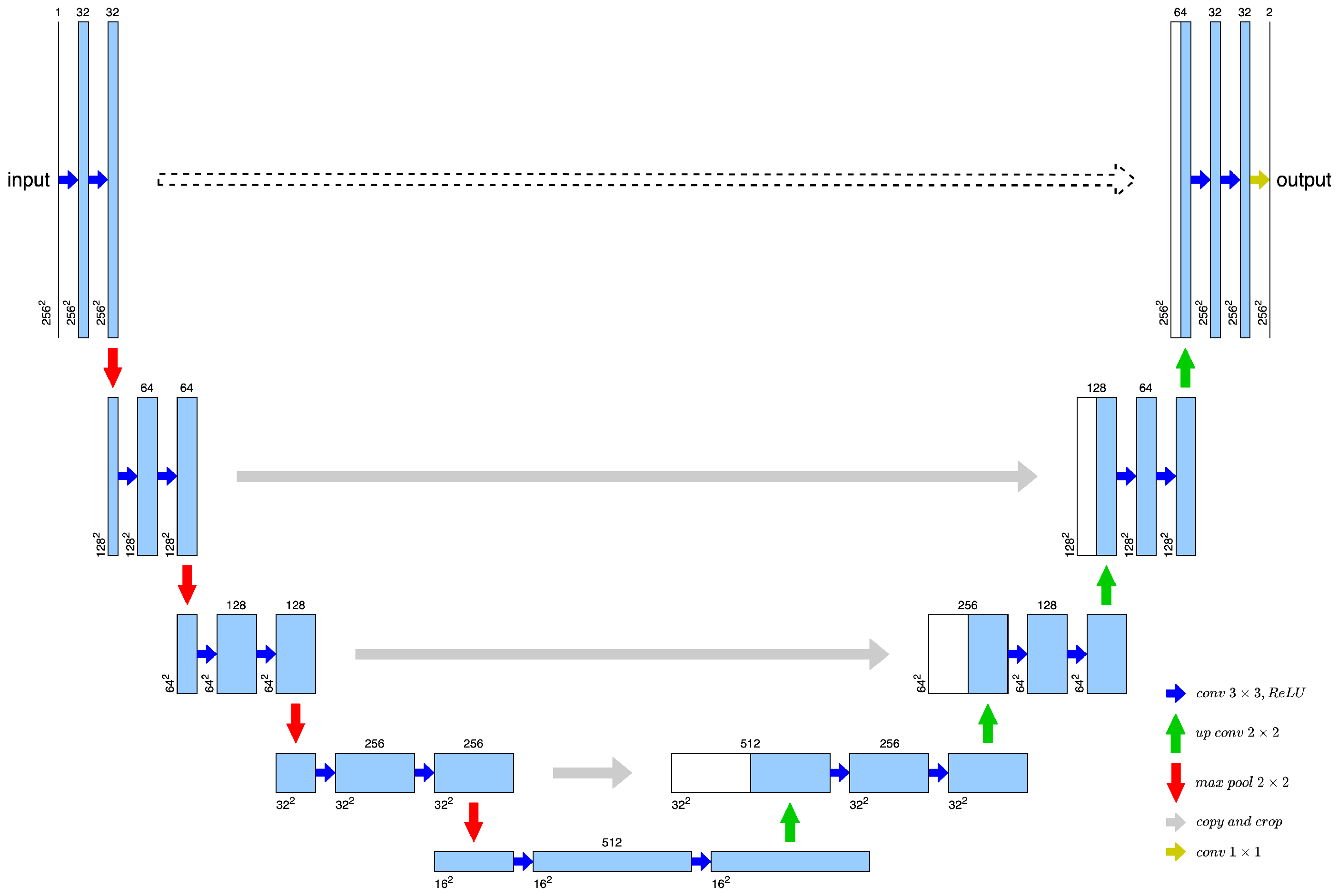
U-Net is an efficient deep learning framework for image segmentation task. As Figure 4 shows, it can be divided into the front and latter part. The front is the downsampling part for feature extraction, which is composed of convolution layer and pooling layer. The latter one is the upsampling part for image reconstruction, which is composed of an up-convolution layer and a convolution layer. It should be noted that the net concatenates the front part and the latter part in each parallel layer, so that more information of feature extraction can be reserved.
For the classical U-Net neuron network, suppose that is the data obtained after upsampling at the i-th layer, is the data before upsampling, is the data mapped from the left side of the network at the i-th layer and C represents the upsampling process. Then its mathematical formula can be expressed as
Our task is to invert seismic waveforms to generate velocity field and anomalies locations. A modified U-Net is proposed with a different structure from the classical one. Initially, the convolution operation starts from 1 pixel outside the edge of the seismic image, which guarantees that the generated velocity field does not change the size while acquiring the features of the original data. In addition, since it is found in the classical U-Net experiments that the generated velocity fields are contaminated by the contour of the seismic waveform, and the reason is that the classical U-Net transmits some parts of the data to the output directly, we modify the classical U-Net structure and omit the transmitted part. The structure of the modified U-Net is shown in Figure 4, and the dashed line indicates the transmitting process in traditional U-Net. The corresponding formulation is as follows:
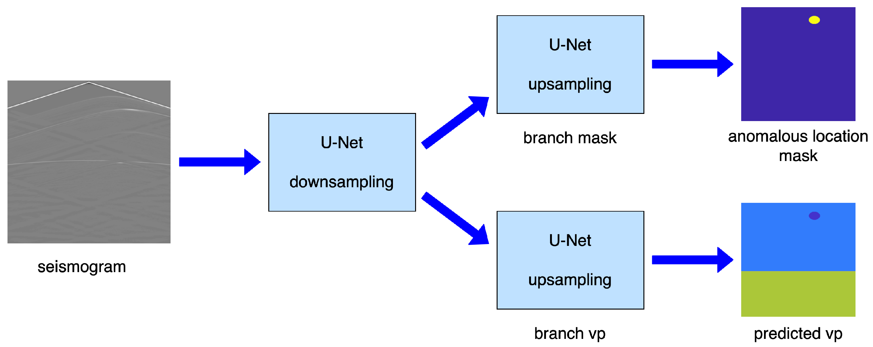
In addition, the upsampling process is divided into two branches, which are used to predict the velocity field and the anomaly mask, respectively. Under this setting, which is shown in Figure 5, the velocity and the anomaly mask can be generated from the corresponding seismic waveform simultaneously.
Velocity field image generation is a regression problem, and the MSE type of loss function is often used. On the other hand, anomaly image generation is a classification problem, where the BCE type of loss function should be employed. Classification and regression problems cannot use the same loss function as the criterion. Therefore, we define an ensemble loss function of the entire U-Net as a weighted summation of MSE and BCE loss with a fine-tunable parameter . The accuracy requirement of the model is that the ensemble loss function is less than a threshold, so that the accuracy of two branches can be guaranteed simultaneously. The ensemble loss function is defined as
2.4. Post-Processing
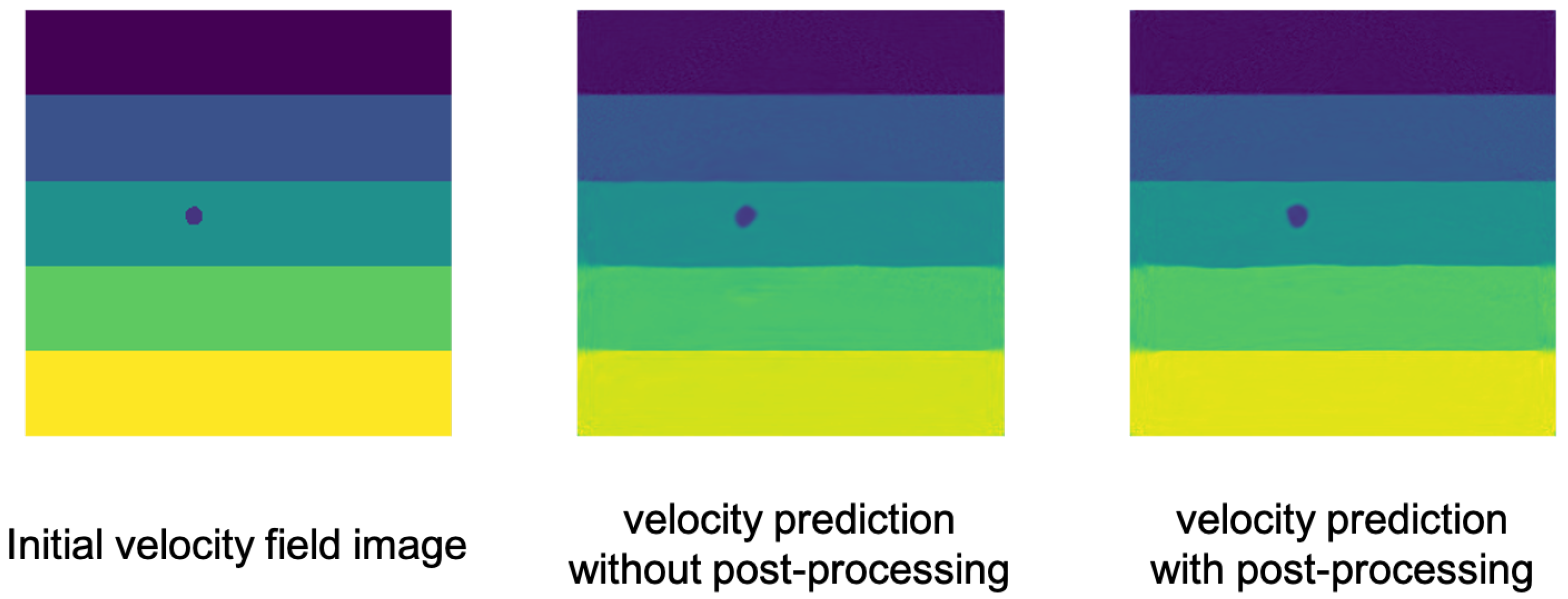
In practice of the Velocity Model Building, geophysicists usually apply a smoothing post-processing step to obtain a more reliable background velocity field. Following this traditional setting, we added two convolutional layers to the generated velocity field image to achieve a smoothing effect. As shown in Figure 6, the velocity field with a post-processing step has a more reasonable background and without touching the anomalies.
3. Results
For an area, the seismic wave propagation speed of different geological structures in the area is different, and there is a cavity in the geological structure (wave velocity is different from other geological structures). In this algorithm, when the data of the velocity field are given, a seismic waveform can be obtained by simulating the ground explosion. The specific method is to input velocity field data and modeling parameters (including shot position, parameters for recording wavefield snapshots, etc.) into the program. Then the corresponding seismic data and seismic waveforms will be generated by using the finite difference method. We made a comparison to the similar machine learning algorithm proposed in [13]. The experiments were performed on a workstation with two 10 Core Intel(R) Xeon(R) Silver 4210R CPU, 2 RTX A5000 GPU, 128GB RAM and an Ubuntu 20.04 operating system that implements Pytorch. The code of our algorithm has been uploaded to GitHub (https://github.com/DavidDeadpool/Unet-seismic/tree/main/Unet-seismic, accessed on 12 July 2022).
First, we generated a set of velocity models with anomalies distributed randomly and also generated the masks to describe the location of the anomalies corresponding to each velocity model. Then we modeled seismic shot gathers based on the generated velocity models. Finally, we paired the shot gathers and the masks together as the input and output of the training pairs of the U-Net network.
3.1. Velocity Models with Anomalies
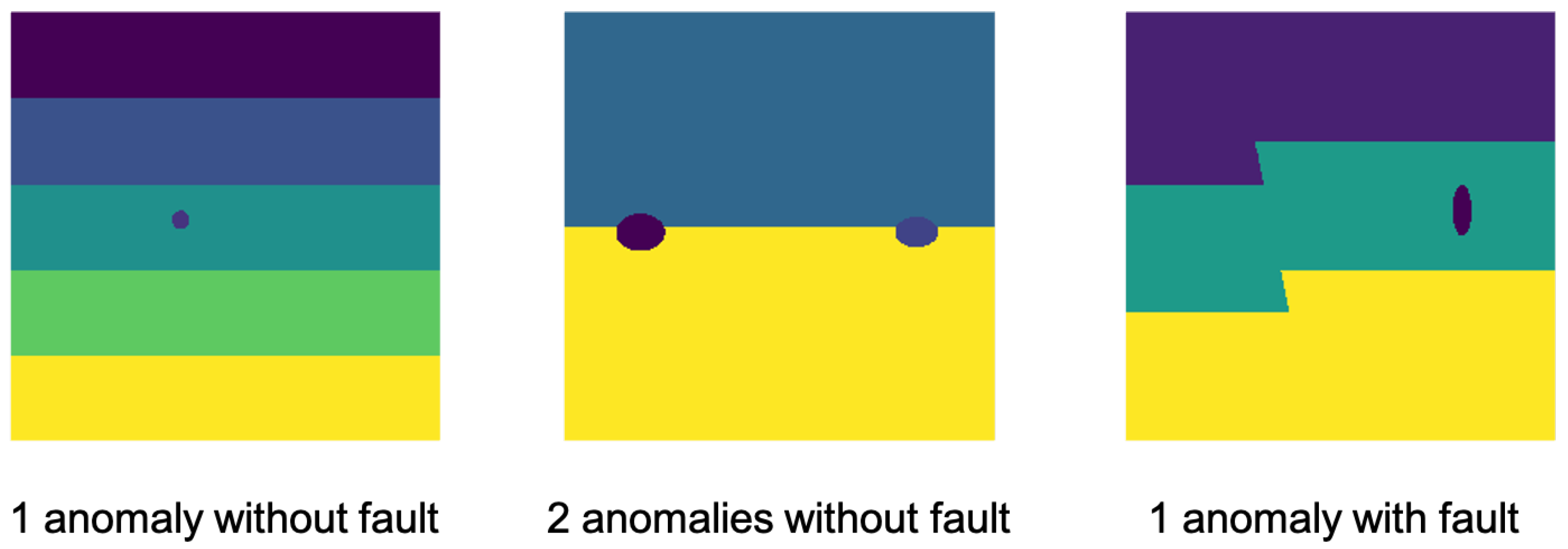
We have generated various types of velocity models. The basic type is a velocity model with one anomaly and no fault. Through the controlled variable method, the other velocity fields are multiple (two) anomalies with no fault and one anomaly with fault. According to the natural laws of geophysics, the velocity in the upper level (near the surface) is small, and the velocity increases as the depth increases. The location and size of the anomalies are randomly generated, and the default shape of the anomaly is an ellipse. The length of the semi-axis of the ellipse is . Figure 7 shows the different types of velocity models.
3.2. Seismic Waveforms
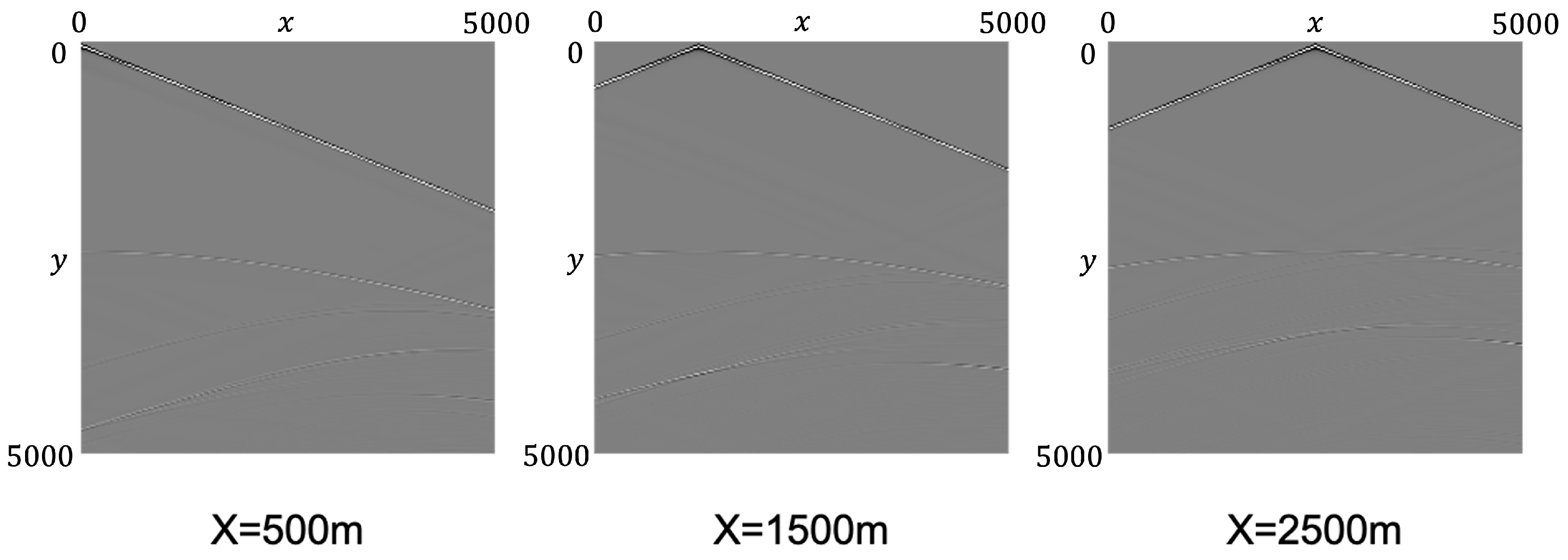
By using a 2D acoustic wave modeling algorithm [18], we calculated the reflection seismic records and wavefield snapshots corresponding to different shot points. We assume that the entire area is 5000 m wide, and the source and receiver position can be in this 5000 m area. The leftmost end of the image is set to m, and the rightmost end is m. We can collect one seismic waveform at each seismic wave launch location. For convenience, for the input of multiple seismic waveforms, the experiment selects the shots at locations of 500 m, 1500 m, 2500 m, 3500 m and 4500 m. Figure 8 shows the seismic waveforms corresponding to different shot positions.
3.3. Results
In order to understand the influence of fault and the number of anomalies on the experimental results, we conducted multiple sets of comparative experiments. In addition, in order to determine the impact of the number of shot points on the accuracy of the experiment, we conducted single shot point experiments ( m) and multiple shot point experiments m, 1500 m, 2500 m, 3500 m, 4500 m) and completed the comparison in each set of comparison experiments.
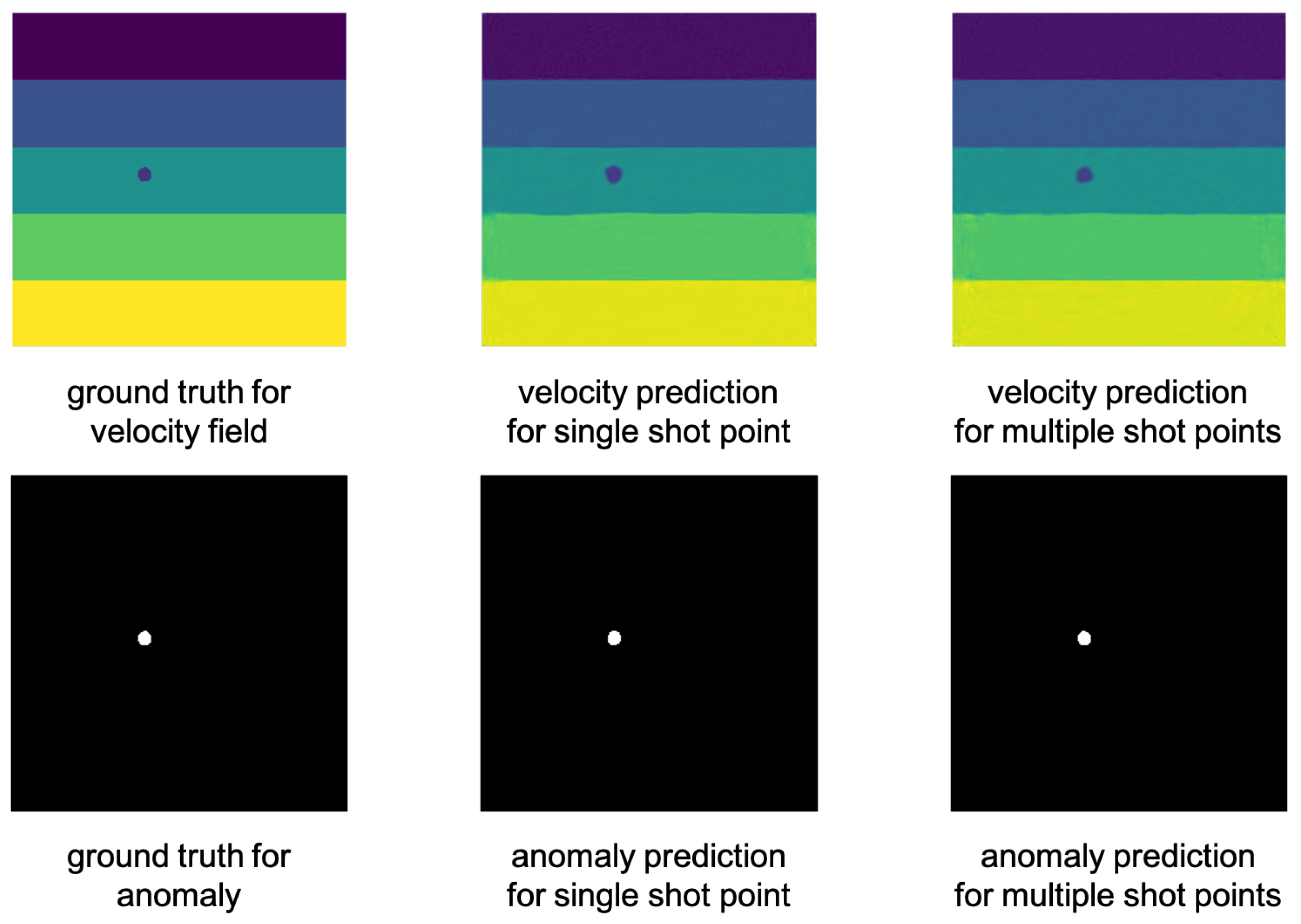
3.3.1. One Anomaly without Fault
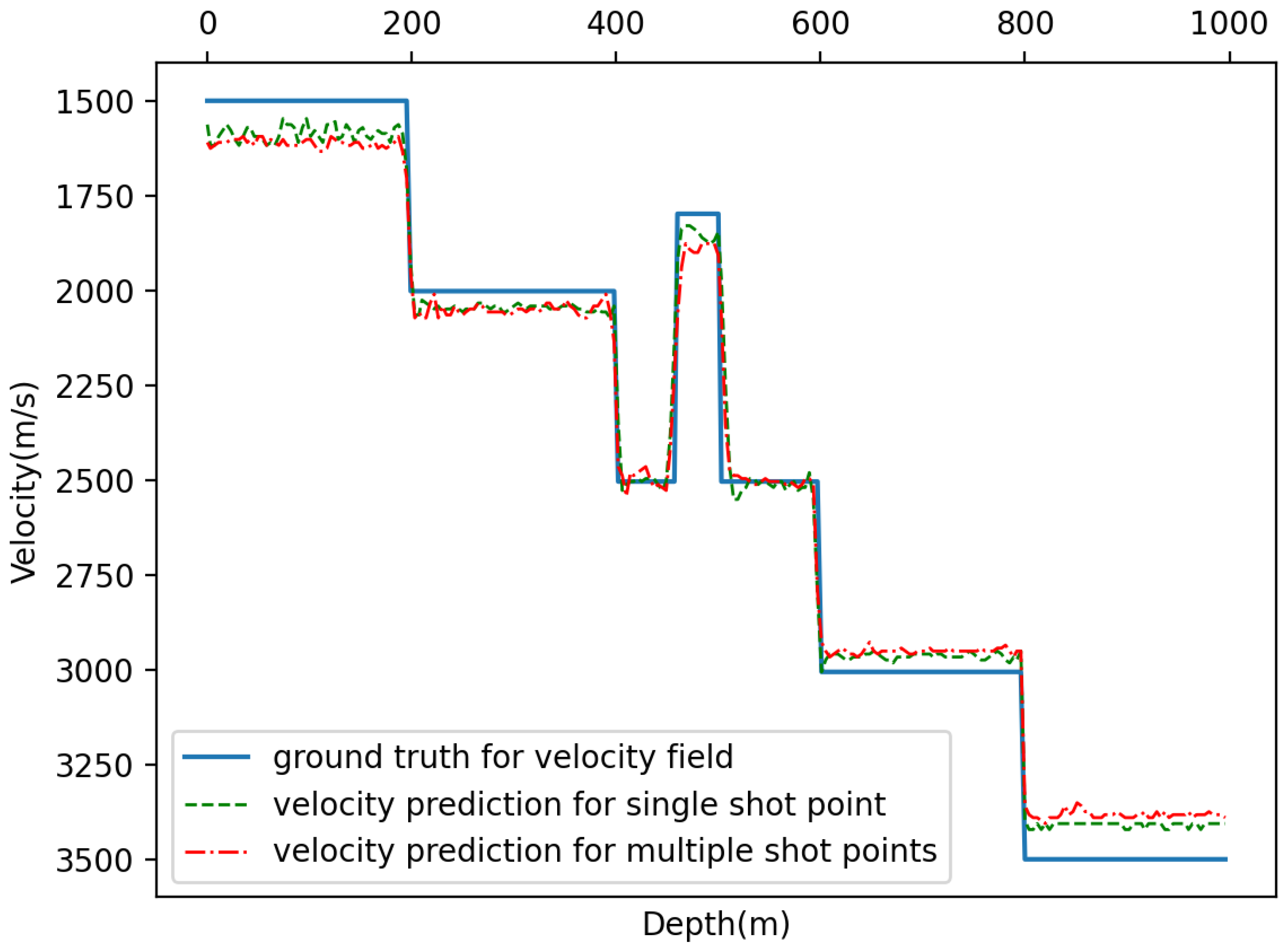
In this group of experiments, the velocity model is divided into five layers without fault, and there is only one anomaly. We made predictions for a single shot point and multiple shot points. The velocity field and anomaly images obtained through training are shown in Figure 9. There is no obvious difference in the prediction of the velocity field. In order to better view the prediction effect of the velocity field, we have produced vertical velocity profiles, as shown in Figure 10. The prediction error of a single shot point at an anomaly is smaller than that of a multi-shot-point prediction.
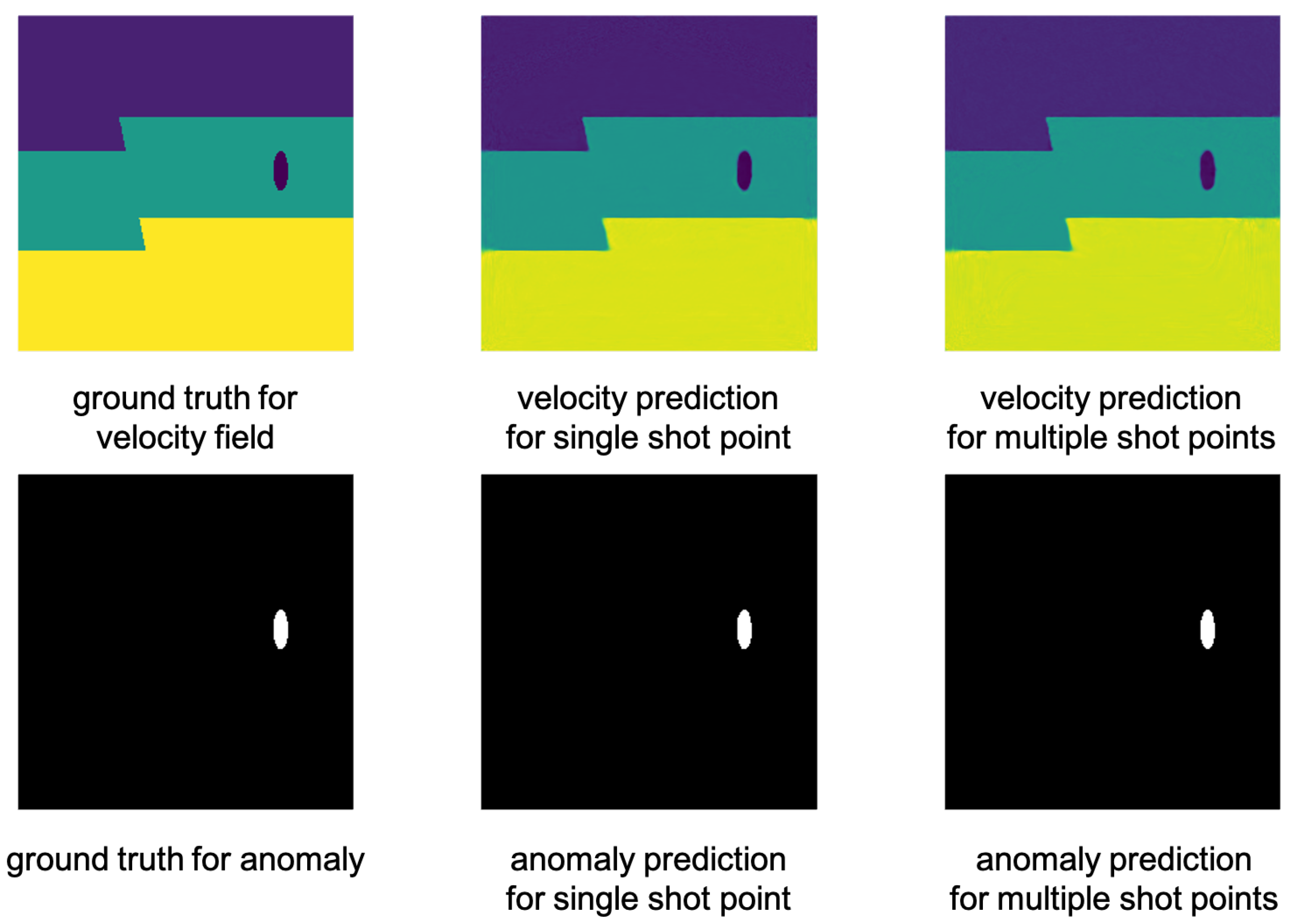
3.3.2. One Anomaly with Fault
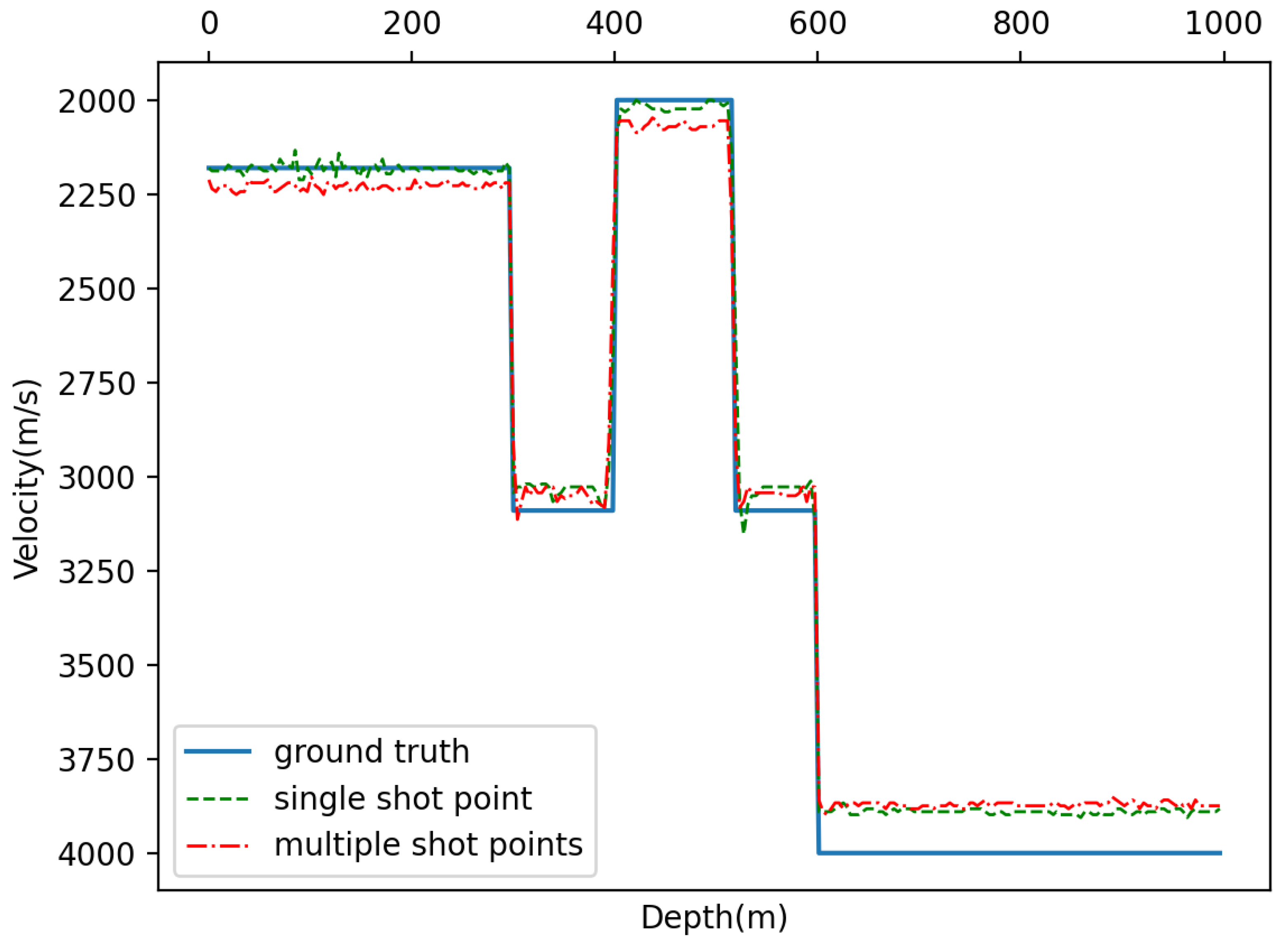
In this group of experiments, the velocity field is divided into three layers, with only one abnormal point. We made predictions for a single shot point and multiple shot points. The effect of predicting the velocity field and abnormal points is shown in Figure 11. There is no obvious difference in the prediction of both velocity field and anomaly. In order to better view the prediction effect of the velocity field, we have produced vertical velocity profiles, as shown in Figure 12. The prediction error of a single shot point at an anomaly is smaller than that of a multi-shot-point prediction.
3.3.3. Multiple Anomaly without Fault
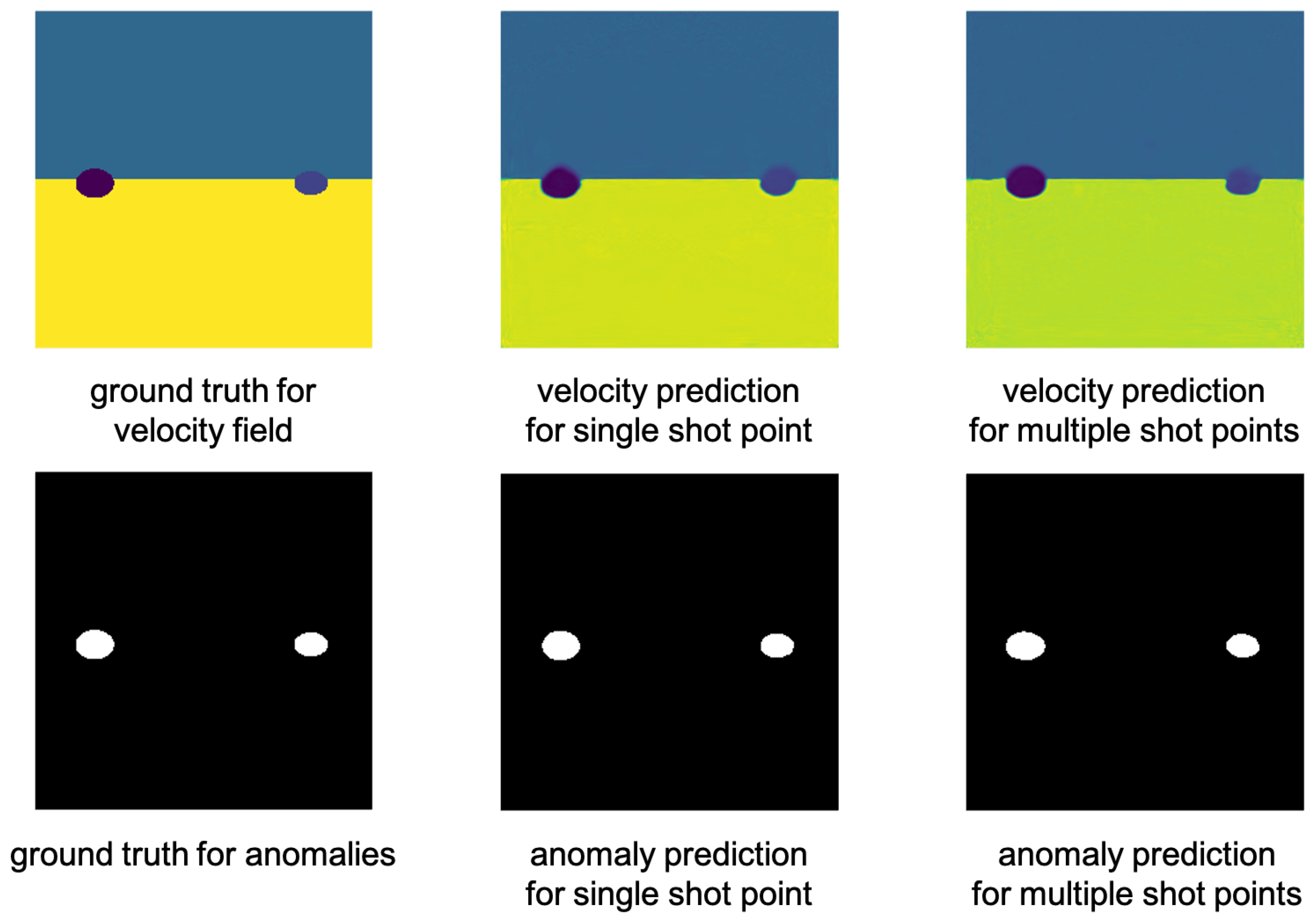
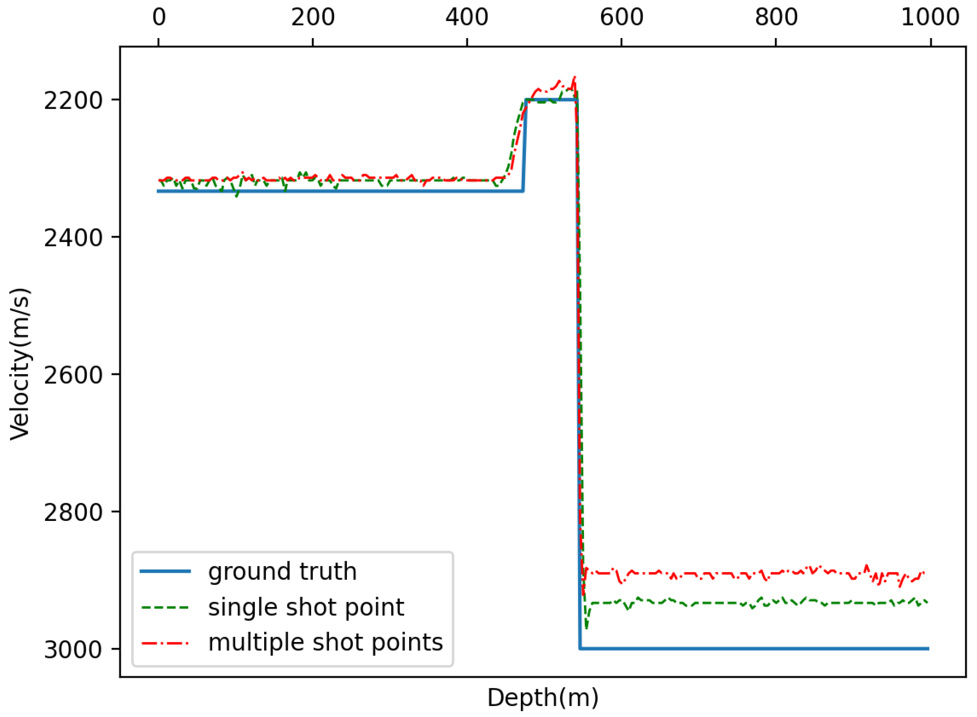
In this group of experiments, the velocity field is divided into two layers, with two anomalies. We made predictions for a single shot point and multiple shot points. The effect of predicting the velocity field and anomalies is shown in Figure 13. There is no obvious difference in the prediction of the velocity field, but the method of single-shot prediction is more accurate for the prediction of anomalies. In order to better view the prediction effect of the velocity field, we have produced vertical velocity profiles, as shown in Figure 14. The prediction error of a single shot point at an anomaly is smaller than that of a multi-shot-point prediction.
In summary, the neural network algorithm based on U-Net can accurately complete the process of predicting the velocity field and anomalies from the seismic waveform. Both single shot point and multiple shot points have good prediction effects, but the effect of multiple shot points is not necessarily better than single shot point.
4. Discussions and Conclusions
We generated simulated seismic data based on the finite difference method and used the modified U-Net to successfully predict the underground velocity field and the location of anomalies from seismic waveforms, and then used CNN to post-process the generated images. Experimental results show that the effect of multi-shot-point prediction is not necessarily better than that of single shot point. After numerical verification, the predicted velocity field and abnormal point position have very little error with the ground truth. It should be noted that traditional VMB normally needs weeks or months to reconstruct the velocity model; however, our algorithm only needs days, which is shown as Table 1. Next, we will use real seismic data to verify and refine our model.
There are still some problems with our model. First of all, as shown in Figure 10, Figure 12 and Figure 14, as the depth increases, the error of the velocity prediction will gradually increase. In addition, the data used in each of our experiments correspond to 1000 sets of artificially generated information. It is necessary to increase the amount of information and use real seismic data to improve the applicability of the model to the actual situation. Finally, although U-Net can extract image features well and achieve the required training effects, this processing is based on images and not directly obtained from seismic data training. The image resolution will seriously affect the training effect. We will continue to find ways to overcome these problems.
Author Contributions
Methodology, J.J. (Jiwei Jia) and J.J. (Jian Jiao); Resources, P.Y.; Software, Z.L. (Ziqian Li); Validation, Z.L. (Zheng Lu); Writing—Original Draft, Z.L. (Ziqian Li). All authors have read and agreed to the published version of the manuscript.
Funding
The authors are supported by the Natural Science Foundation of Jilin Province (Grant No. 20210101481JC), the Shanghai Municipal Science and Technology Major Project (Grant No. 2021SHZDZX0103), and the Fundamental Research Funds for the Central Universities (Grant No. 93K172020K27).
Institutional Review Board Statement
Not applicable.
Informed Consent Statement
Not applicable.
Data Availability Statement
The data that support the findings of this study are available from the corresponding author upon reasonable request.
Conflicts of Interest
The authors declare no conflict of interest.
References
- Rointan, A.; Soleimani Monfared, M.; Aghajani, H. Improvement of seismic velocity model by selective removal of irrelevant velocity variations. Acta Geod. Geophys. 2021, 56, 145–176. [Google Scholar] [CrossRef]
- Shahbazi, A.; Ghosh, D.; Soleimani, M.; Gerami, A. Seismic imaging of complex structures with the CO-CDS stack method. Stud. Geophys. Geod. 2016, 60, 662–678. [Google Scholar] [CrossRef]
- Bouchaala, F.; Guennou, C. Estimation of viscoelastic attenuation of real seismic data by use of ray tracing software: Application to the detection of gas hydrates and free gas. Comptes Rendus Geosci. 2012, 344, 57–66. [Google Scholar] [CrossRef]
- Xin, K.; Hung, B. 3-D tomographic Q inversion for compensating frequency dependent attenuation and dispersion. In SEG Technical Program Expanded Abstracts; Society of Exploration Geophysicists: Houston, TX, USA, 2009; pp. 4014–4018. [Google Scholar]
- Zhou, J.; Birdus, S.; Hung, B.; Teng, K.H.; Xie, Y.; Chagalov, D.; Cheang, A.; Wellen, D.; Garrity, J. Compensating attenuation due to shallow gas through Q tomography and Q-PSDM, a case study in Brazil. In SEG Technical Program Expanded Abstracts; Society of Exploration Geophysicists: Houston, TX, USA, 2011; pp. 3332–3336. [Google Scholar]
- Zhou, J.; Wu, X.; Teng, K.H.; Xie, Y.; Lefeuvre, F.; Anstey, I.; Sirgue, L. FWI-guided Q tomography and Q-PSDM for imaging in the presence of complex gas clouds, a case study from offshore Malaysia. In SEG Technical Program Expanded Abstracts 2013; Society of Exploration Geophysicists: Houston, TX, USA, 2013; pp. 4765–4769. [Google Scholar]
- Zhang, Z.; Jia, J.; Fu, G.; Zhang, H.; Chow, D.; Hung, B.; Anstey, I.; Lai, W.L. Fullband Imaging. 2016. Available online: https://archives.datapages.com/data/petroleum-exploration-society-of-australia/news/140/140001/pdfs/52.htm (accessed on 12 July 2022).
- Matsushima, J.; Ali, M.Y.; Bouchaala, F. A novel method for separating intrinsic and scattering attenuation for zero-offset vertical seismic profiling data. Geophys. J. Int. 2017, 211, 1655–1668. [Google Scholar] [CrossRef]
- Hinton, G.E. Deep belief networks. Scholarpedia 2009, 4, 5947. [Google Scholar] [CrossRef]
- Guillen, P.; Larrazabal, G.; González, G.; Boumber, D.; Vilalta, R. Supervised learning to detect salt body. In SEG Technical Program Expanded Abstracts; Society of Exploration Geophysicists: Houston, TX, USA, 2015; pp. 1826–1829. [Google Scholar]
- Guillen, P.; Larrazabal, G.; Gonzalez, G.; Sineva, D. Detecting salt body using texture classification. In Proceedings of the 14th International Congress of the Brazilian Geophysical Society & EXPOGEF, Rio de Janeiro, Brazil, 3–6 August 2015; Society of Exploration Geophysicists: Houston, TX, USA, 2015; pp. 1155–1159. [Google Scholar]
- Hastie, T.; Tibshirani, R.; Friedman, J. The Elements of Statistical Learning: Data Mining, Inference, and Prediction; Springer Science & Business Media: Berlin/Heidelberg, Germany, 2009. [Google Scholar]
- Zhang, C.; Frogner, C.; Araya-Polo, M.; Hohl, D. Machine-learning based automated fault detection in seismic traces. In Proceedings of the 76th EAGE Conference and Exhibition, Amsterdam, The Netherlands, 16–19 June 2014; Volume 2014, pp. 1–5. [Google Scholar]
- Cohen, I.; Coult, N.; Vassiliou, A.A. Detection and extraction of fault surfaces in 3D seismic data. Geophysics 2006, 71, P21–P27. [Google Scholar] [CrossRef] [Green Version]
- Hale, D. Methods to compute fault images, extract fault surfaces, and estimate fault throws from 3D seismic images. Geophysics 2013, 78, O33–O43. [Google Scholar] [CrossRef]
- Long, J.; Shelhamer, E.; Darrell, T. Fully convolutional networks for semantic segmentation. In Proceedings of the IEEE Conference on Computer Vision and Pattern Recognition, Boston, MA, USA, 7–12 June 2015; pp. 3431–3440. [Google Scholar]
- Ronneberger, O.; Fischer, P.; Brox, T. U-net: Convolutional networks for biomedical image segmentation. In International Conference on Medical Image Computing and Computer-Assisted Intervention; Springer: Berlin/Heidelberg, Germany, 2015; pp. 234–241. [Google Scholar]
- Artru, J.; Farges, T.; Lognonné, P. Acoustic waves generated from seismic surface waves: Propagation properties determined from Doppler sounding observations and normal-mode modelling. Geophys. J. Int. 2004, 158, 1067–1077. [Google Scholar] [CrossRef]
Figure 1.
Flow chart.

Figure 2.
Training procedure.

Figure 3.
Verification procedure.

Figure 4.
Architecture of the modified U-Net neuron network.

Figure 5.
U-Net separated into 2 parts.

Figure 6.
Post-processing step.

Figure 7.
Examples of velocity models.

Figure 8.
Seismic waveforms at different shot positions.

Figure 9.
Prediction for velocity field and anomaly in velocity model with one anomaly and no fault.
Figure 9.
Prediction for velocity field and anomaly in velocity model with one anomaly and no fault.

Figure 10.
Vertical velocity profiles of velocity field with one anomaly and no fault.

Figure 11.
Prediction for velocity field and anomaly with one anomaly and fault.

Figure 12.
Vertical velocity profiles of velocity field with one anomaly and fault.

Figure 13.
Prediction for velocity field and anomaly with 2 anomalies and no fault.

Figure 14.
Vertical velocity profiles of velocity field with 2 anomalies and no fault.


Table 1.
Time of calculation in one anomaly without fault experiment.
| Experiment | Time of Training | Time of Prediction |
|---|---|---|
| Single shot point | 95.3 h | 5 min |
| Multiple shot points | 109.3 h | 5 min |
Publisher’s Note: MDPI stays neutral with regard to jurisdictional claims in published maps and institutional affiliations. |
© 2022 by the authors. Licensee MDPI, Basel, Switzerland. This article is an open access article distributed under the terms and conditions of the Creative Commons Attribution (CC BY) license (https://creativecommons.org/licenses/by/4.0/).
Share and Cite
MDPI and ACS Style
Li, Z.; Jia, J.; Lu, Z.; Jiao, J.; Yu, P. Seismic Velocity Anomalies Detection Based on a Modified U-Net Framework. Appl. Sci. 2022, 12, 7225. https://0-doi-org.brum.beds.ac.uk/10.3390/app12147225
AMA Style
Li Z, Jia J, Lu Z, Jiao J, Yu P. Seismic Velocity Anomalies Detection Based on a Modified U-Net Framework. Applied Sciences. 2022; 12(14):7225. https://0-doi-org.brum.beds.ac.uk/10.3390/app12147225
Chicago/Turabian StyleLi, Ziqian, Jiwei Jia, Zheng Lu, Jian Jiao, and Ping Yu. 2022. "Seismic Velocity Anomalies Detection Based on a Modified U-Net Framework" Applied Sciences 12, no. 14: 7225. https://0-doi-org.brum.beds.ac.uk/10.3390/app12147225
Note that from the first issue of 2016, this journal uses article numbers instead of page numbers. See further details here.