
Estimation of Litho-Fluid Facies Distribution from Zero-Offset Acoustic and Shear Impedances


1
Department of Geosciences, Universiti Teknologi Petronas, Seri Iskander 32610, Perak, Malaysia
2
The Institute of Digital Signal Processing, University of Duisburg-Essen, Forsthausweg 2, 47057 Duisburg, Germany
*
Author to whom correspondence should be addressed.
Appl. Sci. 2022, 12(15), 7754; https://0-doi-org.brum.beds.ac.uk/10.3390/app12157754
Submission received: 8 June 2022
/
Revised: 5 July 2022
/
Accepted: 5 July 2022
/
Published: 1 August 2022
(This article belongs to the Special Issue Technological Advances in Seismic Data Processing and Imaging)
Abstract
:Seismic data are considered crucial sources of data that help identify the litho-fluid facies distributions in reservoir rocks. However, different facies mostly have similar responses to seismic attributes. In addition, seismic anisotropy negatively affects the facies predictors extracted from seismic data. Accordingly, this study aims at estimating zero-offset acoustic and shear impedances based on partial-stack inversion by two methods: statistical modeling and a multilayer feed-forward neural network (MLFN). The resulting impedance volumes are compared to those obtained from isotropic simultaneous inversion by using impedance logs. The best impedance volumes are applied to Thomsen’s anisotropy equations to solve for the anisotropy parameters Epsilon and Delta. Finally, the shear and acoustic impedances are transformed into elastic properties from which the facies and fluid distributions are predicted by using the logistic regression and decision tree algorithms. The results obtained from the MLFN show better matching with the impedance and facies logs compared to those obtained from isotropic inversion and statistical modeling.
1. Introduction
Seismic data have proved to be important quantitative tools that can bring valuable information about rock properties, especially when being integrated with statistical tools. For example, multiattribute transforms were used to predict log properties from seismic data [1]. Another common approach is to invert seismic data into elastic properties and then into petrophysical properties by statistical relationships obtained from logging data [2]. Porosity, lithology, and fluid properties were also estimated with the resampling of rock physics constraints [3,4,5]. Russel used multivariate statistics and neural networks to predict reservoir parameters from seismic attributes [6]. In addition, Bachrach inverted porosity and water saturation by stochastic rock physics modeling [7].
Other methodologies consider reservoir parameter inversion based on Bayesian classification theory [8,9]. Moreover, a geostatistical inversion method was used to predict reservoir properties in a higher certainty than that of deterministic methods [10]. In addition, some studies derived elastic properties from prestack seismic inversion to define facies [11,12]. Another straightforward methodology is to combine petroelastic modeling and stochastic inversion to predict hydrocarbon zones based on Bayesian theory [13]. A rock physics model was postulated to derive the elastic rock properties from mineral parameters and structure information [14]. Recently, rock properties were estimated from angle stack seismic data by a Bayesian inversion based on the Gibbs sampling algorithm [15].
Machine learning (ML) tools have been widely used in reservoir characterization [16]. For instance, formation porosity and permeability were estimated from logging and core data by using an artificial neural network (ANN) [17,18,19]. Other studies also used neural networks to predict essential rock properties such as permeability [20,21,22] and shear wave velocity [23,24,25,26]. Neural networks can be combined with seismic attributes to predict rock physics properties from seismic data [27,28,29,30]. In addition, facies distributions were estimated by both supervised and unsupervised ML algorithms such as ANN [31,32], convolutional neural network (CNN) [33,34,35], support vector machine (SVM) [36,37,38,39,40,41], bagged tree (BT) [42,43], relevance vector machine (RVM) [44], seed region growing (SRG) [45], self-organizing map (SOM) [46,47], principal component analysis (PCA) [48,49,50], and generative topographic mapping (GTM) [51]. Some challenges are common in ML facies models such as over-fitting and over-parametrization. Moreover, such models should consider the limitations of seismic data to eliminate error as much as possible. One of the problems that contributes to the uncertainty of seismic-derived methods is seismic anisotropy.
This study aimed at forecasting zero-offset P-impedance () and S-impedance () by using statistical modeling and MLFN after applying a partial-log-constrained inversion to the near, mid, and far angle stacks. The outputs of this objective were zero-offset impedances that were more accurate than those obtained from isotropic simultaneous inversion. Another objective was to compare the abilities of both statistical modeling and neural networks to turn the randomness of the data into identified patterns. The next step was to apply the best and volumes to Thomsen’s anisotropy equations to solve for the anisotropy parameters, Epsilon and Delta, assuming a vertical transverse isotropic (VTI) medium. Next, the zero-offset and were used as inputs to a facies model, which predicted the distribution of three classes: gas sand, wet sand, and shale. The idea of the facies model is to forecast the sand and gas probabilities by logistic regression [52] and then use them as inputs for a decision tree to predict the distribution of each facies class.
The three offset stacks were converted into angle stacks, which were the inputs of the partial-stack inversion, and angle gathers, which were the inputs of the simultaneous isotropic inversion. The ranges of the near, mid, and far stacks were from 5° to 15°, 15° to 25°, and 25 to 40°. The partial-stack inversion resulted in the and volumes at the central angles, 10°, 20°, and 32.5°, from which the zero-offset properties were forecasted. The target zone consisted of two gas-bearing shaly sand reservoirs in the Malay basin: A and B. The training data of the Bayesian and MLFN models were gathered from the wells (×1) and (×2); however, the facies log was only obtained at the well (×1) due to the availability of the petrophysical cut-offs and oil-mud resistivity imaging data. Another challenge was that the log was only available at the well (×1), so it was estimated from other log properties by the MLFN neural network at the well (×2).
The resulting and were compared to those obtained from isotropic inversion by using the impedance logs. The MLFN resulted in the most accurate zero-offset impedances. Therefore, the and volumes were applied to Thomsen’s anisotropy equations to solve for the anisotropy parameters Epsilon and Delta. The and of MLFN and isotropic inversion were transformed into the near and far elastic impedances, which were the lithology predictors, and then into the Mu–Rho (MR) ratio, Lambda–Rho/Mu–Rho (LR/MR) ratio, and Poisson’s ratio (PR), which are the fluid predictors. The litho-fluid model was applied to the inverted elastic volumes to forecast the litho-fluid facies distribution. The facies log was used to validate the predicted facies obtained from the isotropic and anisotropic approaches.
2. Seismic Anisotropy
Seismic anisotropy is the dependence of the seismic velocity on the incident angle [53,54,55]. Wave propagation in anisotropic media has been discussed by various studies [53,56,57,58]. To understand the seismic anisotropy of the Earth’s subsurface, the relationship between the internal forces (stress) and deformation occurring in the medium (strain) should be defined. When an elastic wave propagates through the subsurface, the stress–strain relationship can be obtained according to Hooke’s law as shown below [59]:
where is the stress tensor, is the strain tensor, and is the elastic (stiffness) tensor, which is a fourth-order tensor with 81 independent components. Both the strain and stress tensors are symmetric [60], resulting in:
The 81 independent components are accordingly reduced to 36 due to the symmetry in the stress and strain tensors. Therefore, the elastic tensor () is replaced with a 6 × 6 matrix (), where [61]:
where and are the new indices of the elastic tensor. The resulting (6 × 6) notation matrix is expressed as shown below:
There are several types of symmetry for the independent components that determine the degree of anisotropy. The maximum anisotropy degree occurs at the lowest possible symmetry, which is called “triclinic” symmetry and occurs when the () matrix has 21 different nonzero components, which is considered the maximum number of elements required to describe an anisotropic medium [58]. On the other hand, the isotropic case occurs at the highest symmetry case with a smaller amount of independent components.
The most realistic symmetry case of the Earth’s subsurface is polar symmetry, which has a single pole of rotational symmetry (Z-axis) that is different from the other two axes (X and Y) [61]. This anisotropy case is called transverse isotropy (TI), at which rock properties are assumed invariant about an axis of symmetry. If the symmetry axis is vertical, this means that the layers are considered horizontal and is hence called vertical transverse isotropy (VTI). Another case is called tilted transverse isotropy (TTI), which is a more realistic case because it follows the variations of the dip angles of layers. Polar symmetry can be described by a matrix of five different independent components, as shown below:
There are three anisotropy parameters that can define any anisotropy degree in terms of the stiffness components of a TI medium [53]. The anisotropy parameters are called Epsilon (), Delta (), and Gamma (). The weaker the anisotropy degree is, the closer these parameters are to zero. The anisotropy parameters in the weak anisotropy case have values less than 1.
Epsilon is the fractional difference between the vertical and horizontal P-wave velocities. It generally has a positive sign because rocks are less compressible along bedding than across bedding. It can be obtained by the following equation:
where is the anisotropy parameter Epsilon, is the horizontal P-wave velocity, is the vertical P-wave velocity, and and are the stiffness components of the elastic tensor.
The Delta parameter controls the near-vertical anisotropy and does not relate to the horizontal velocity, so it can be positive or negative. Assuming weak anisotropy, the Delta parameter refers to the stiffness components by the following equation:
where is the anisotropy parameter Delta, while , , and are the stiffness components of the elastic tensor.
The Gamma parameter is the fractional difference between the vertical and horizontal S-wave velocities and can be given as follows:
where is the anisotropy parameter Gamma, is the horizontal S-wave velocity, is the vertical S-wave velocity, and and are the stiffness components of the elastic tensor.
The P- and S-wave velocities can be defined in terms of the anisotropy parameters based on the weak anisotropy assumption [53,61], as shown below:
where ) and ) are the vertical P-wave and S-wave velocities, respectively, ) is the horizontal S-wave velocity, and are the zero-offset P-wave and S-wave velocities, respectively, at = 0, and is the incident angle.
3. The Effect of Seismic Anisotropy on Seismic Data
Seismic anisotropy causes a misinterpretation of seismic data, which affects the final reservoir model. For example, if seismic anisotropy is neglected, a target may be expected at the wrong depth. Another problem is that seismic anisotropy affects the angle-dependent reflectivity calculation, which is further used for prestack seismic applications such as amplitude versus offset (AVO) and elastic impedance (EI). Figure 1 shows a comparison between the isotropic and anisotropic assumptions, which yield significantly different reflectivities at the top of the C-sand reservoir in the Sawan gas field [62]. In addition to that, seismic anisotropy adds uncertainty to prestack seismic inversion, which results in inaccurate rock properties.
A common workflow of anisotropic seismic inversion is to obtain the anisotropy parameters and then process seismic data before the inversion process. The anisotropy parameters can be obtained from various types of data. However, the most confident sources of anisotropy quantification are core data. Traditional laboratory ultrasonic measurements of intrinsic anisotropy [63] depend on a limited number of orientations, resulting in inaccurate anisotropy measurements. On the other hand, more effective methods [64,65,66,67] depend on many ray paths having various inclination angles to the bedding plane.
A numerical study was applied to ultrasonic measurements according to Markov chain Monte Carlo simulation (MCMC) [68]. The idea of this study was to obtain the probability distribution curves of the anisotropy parameters based on the layering effects of five lithofacies: dry sandstone, wet sandstone, dry carbonate, wet carbonate, and shale. Accordingly, the anisotropy parameters were simulated for each facies class. The Backus averaging method helped calculate the harmonic means of the anisotropy parameters, assuming a horizontally layered inhomogeneous medium [69].
Another source of anisotropy information is the vertical seismic profile (VSP). For instance, one study aimed at obtaining the horizontal slowness (Sx) as well as the vertical slowness (Sz) and then combining them in the vector way to yield the scalar slowness [70,71]. This method results in accurate arrival time and depth values, but it assumes that layers are homogeneous and horizontal, which is not realistic [61].
The Delta parameter was estimated by using both prestack time data and sonic logs [72]. Moreover, a method, called The Empirical Relationship relates the anisotropy parameters to the shale volume (Vsh) that causes the intrinsic anisotropy [73,74,75]. The volume fraction and degree of compaction are assumed to be the controlling factors of the orientation of clay minerals and hence the anisotropy parameters. This method is convenient for heterogeneous media because it solves for the intrinsic anisotropy components. However, the problem of obtaining an accurate zero-offset velocity away from wells still exists. Another study considered the intrinsic anisotropy in shale based on an orientation distribution function [76]. This study aimed at modeling anisotropic elastic properties based on two approaches. The first approach was to apply an anisotropic differential effective medium model (DEM) based on the textural information about the kerogen network in kerogen-rich shale. The second approach was to use the DEM model with a compaction-dependent orientation distribution function to study the anisotropy in laminated shaly sand rocks.
The anisotropic elastic constants were estimated as functions of the fluid-filled porosity and the aspect ratio of the inclusions [77]. Another study introduced an anisotropic dual porosity (ADP) model to forecast the elastic properties of shaly sand rocks based on a combination of the anisotropic formulations of self-consistent approximation (SCA), DEM, and anisotropic Gassmann theory [78].
Kelter also estimated both Epsilon and Delta from synthetic modeling through some algorithms such as neural networks and regridding inversion [56]. The idea of this method is to model synthetics by using a PP and PS survey such that layer boundaries and material properties are predefined, and then the survey is simulated by the ray tracing method to generate a synthetic model from which the anisotropy parameters are forecasted. The best parameter estimates are selected according to the comparison between the synthetic model and the real seismic data. This method gives reliable results but only at well locations.
Another method was set by Liner and Fe [79], who estimated Thomsen’s parameters from routine well logging data, following a theoretical framework which uses sonic logs to provide a fine-layered isotropic elastic model that can be used to calculate anisotropy parameters as functions of depth and seismic wavelength [80]. Thomsen’s parameters can be also estimated from the average velocity, obtained from sonic data, and the mean inclination angles of deviated wells [81]. However, the results of that study were inaccurate because most of the wells’ inclination angles were below 5, showing no anisotropy effect on seismic data. The residual moveout analysis of diving waves has been used to estimate anisotropy parameters by applying different parametrization scenarios [82]. This method is reasonably accurate even for large values of velocity gradients, but it assumes that the velocity increases linearly with depth, while the anisotropy parameters do not. However, this assumption can only apply to homogeneous media.
The previous methods can be used to obtain the anisotropy parameters and then process seismic data to obtain zero-offset images, which can be inverted into accurate rock properties. However, a different approach is to transform the layer properties, obtained from isotropic inversion, into zero-offset parameters based on Ruger’s reflectivity function in horizontal transverse isotropy (HTI) media [83]. Another anisotropic prestack seismic inversion [84] is based on the Markov random field (MRF), which can establish dependencies between the spacial wave propagation field’s nodes based on prior constraints [85]. The weights of those constraints have been optimized by the anisotropic diffusion method to remove the anisotropy effect in three different models: the symmetrical, vertical asymmetrical, and asymmetrical models. This method has produced encouraging results for Vp, Vs, and density.
Based on the elastic wave equation, the anisotropic elastic waveform inversion was applied to invert for the P- and S-wave velocities, density, and Thomsen’s parameters [86]. The method is based on the idea of eliminating the error between the synthetic and field seismic waveform data according to a misfit function [87]. The anisotropic inversion outputs were successfully used to reduce the ground-roll noise in 2D seismic data.
Another methodology depends on multiscale phase inversion, assuming an anisotropic medium [88]. The advantage of this method is that it avoids the nonlinearity of the misfit functions [89] by adding wave-number details to the velocity model by a skeletonized inversion. This method assumes a VTI medium with Delta equal to zero, while the zero-offset P-wave velocity and Epsilon are inverted, resulting in more accurate results compared to full-wave inversion.
It can be concluded that most of the previous methods have quantified seismic anisotropy only at well locations. The interpolation of the anisotropy parameters between wells is challenging and should be further linked to the effect of the facies distribution. Therefore, the current study has improved a previous anisotropic inversion approach [90] which solves for the zero-offset impedances and anisotropy parameters, Epsilon and Delta, based on partial-stack inversion and Thomsen’s anisotropy equations [91]. On the other hand, our study estimates and based on statistical modeling and MLFN rather than calculating them empirically.
The advantage of ML algorithms is that they reduce the random error of partial-stack inversion and result in accurate impedances that best match the logs. Another contribution is that the facies model uses logistic regression to model lithologies and fluids and then combines them using the decision tree algorithm. The integration of two ML algorithms adds stability to the model and raises the chance of being applied to other fields. Moreover, the model includes the depth variable, which acts as a trend factor that highly affects the facies distribution.
4. Methodology
The study workflow, as shown in Figure 2, begins with inverting the angle gathers into , , and density volumes and inverting the angle stacks into and volumes at the near, mid, and far incident angles. Next, the partially inverted impedances are used to forecast the zero-offset impedances by the statistical and MLFN models. The impedance volumes are then compared to each other by using the impedance logs. The best and volumes are applied to Thomsen’s anisotropy equations to solve for the anisotropy parameters, Epsilon and Delta. The next step is to transform the impedance and density volumes into the elastic volumes, from which the sand and gas probabilities are estimated by using the logistic regression model. These probabilities are then inserted into a decision tree model to forecast the distribution of the facies classes: gas sand, wet sand, and shale. The inversion processes in our study were carried out by using the Hampson–Russel software provided by the CGG company.
This study is not applicable to poststack data. The impedance model’s accuracy depends on the seismic data quality as well as the angle gathers’ range. The wider the angle range, the more enhanced signal-to-noise ratio and hence the more accurate the model. Moreover, both the P- and S-impedances should be available in order to solve for the anisotropy parameters: Epsilon and Delta. The study assumes a VTI medium which neglects some anisotropy-related factors such as the layers’ dip angles and fractures; however, impedance modeling by MLFNs accurately solves for the zero-offset impedances by normalizing the error and mitigating the anisotropy effect simultaneously. The study’s facies model is only applicable to the three facies classes: gas sand, wet sand, and shale. However, the model can be extended to include more classes. Moreover, the applicability of the model to other fields can be enhanced if there are more facies data available from a large number of wells.
4.1. Isotropic Simultaneous Inversion
Simultaneous inversion is a prestack seismic inversion that simultaneously inverts the angle gathers into the reflectivities of the , , and density based on the linear relationships between the and each of the and density. The methodology used in this study [92] directly inverted for the , , and density [93,94].
The Aki–Richards equation [95] is an approximation of the relationship between the P-wave reflectivity between two media and the incident angle as follows:
where is the P-wave reflectivity at an incident angle (), while V, W, and are the average P-wave velocity, S-wave velocity, and density between the two media, respectively. The idea of Fatti’s equation [93] is to re-express the Aki–Richards equation in (12) in terms of the acoustic and shear impedances as follows:
where I is the acoustic impedance, J is the shear impedance, the term () is the zero-offset P-wave reflectivity, and the term () is the zero-offset S-wave reflectivity, such that:
Fatti’s equation could be re-expressed by replacing the reflectivities by the rock properties as follows:
where s() is the angle trace, W() is the angle-dependent wavelet, D is a derivative operator, is the acoustic impedance, is the shear impedance, is the density, and is the incident angle. The terms , , and are given by:
where , , and are constants, is the incident angle, is the S-wave velocity, and is the P-wave velocity.
Next, the terms (), (), and () were coupled by the following equations:
where k and m are the intercepts of the linear relations and and are constants, while and () are controlled by the deviations away from the best-fit lines of the linear relationships. and are the displacements of () and () due to the deviation from the best-fit lines.
The next step was to apply the derivative operator (D) to Equations (3) and (4):
where D is the derivative operator, while k and m are the intecepts of the linear relations. Eventually, the algorithm was applied to an initial guess and then iterated until it reached a solution at which the initial model matched the real data with the least-squared error.
4.2. Partial-Log-Constrained Inversion
The separate inversion of angle stacks is based on a partial inversion approach that obtains the zero-offset P- and S-wave velocities from the inverted P- and S-waves at different angular ranges [90]. The idea is based on Thomsen’s equations in (9) and (10), which relate the vertical P-wave () and S-wave () velocities to the anisotropy parameters, Epsilon and Delta, in VTI media.
Partial-log-constrained inversion requires a wavelet to be extracted from each angle stack so that the wavelet is centered at the average angle of the angle stack [90]. An initial model was created from logging data to guide the inversion. This method required S-wave velocity logs in the initial model to constrain the inversion. Each partial seismic volume was inverted into a velocity volume at the central angle of its angle range. Next, the velocity-domain Thomsen’s equations in (9) and (10) were used to solve for the zero-offset P- and S-wave velocities as well as the Epsilon and Delta parameters, as shown in the following equations:
where is the zero-offset P-wave velocity, and are the anisotropy parameters, is the quasivertical P-wave velocity, is the incident angle, and n is the number of partial stacks.
where is the zero-offset P-wave velocity, and are the anisotropy parameters, is the quasivertical S-wave velocity, is the incident angle, and n is the number of the partial stacks.
The log-constrained inversion of partial stacks was adopted from the nonlinear optimization inversion [90], such that the objective function is obtained by:
where V is the inverted P- or S-wave velocity, D is the angle-domain seismic data, and S is the corresponding prediction, which can be expressed according to the convolution model [96]. The reflectivity function is based on the Aki and Richard approximation of the angle-dependent reflectivity [97], as shown below:
where is the reflectivity at an incident angle , while is the zero-offset reflectivity, which is given by:
where , , and are, respectively, the average P-wave velocity, S-wave velocity, and density of the underlying and overlying layers, while , , and are the differences between these properties at the underlying and overlying strata.
The term can be obtained by Gardner’s equation as follows [98]:
According to Equations (24)–(28), the reflectivity will be as follows:
After inverting the partial stacks separately into and volumes at the near, mid, and far angles, the zero-offset velocities Epsilon and Delta were solved by Equations (21) and (22).
The current study applied the same methodology to and by replacing the velocities of Equations (9) and (10) by impedances, as shown below:
Partial inversion is sensitive to the quality of seismic data because the magnitude of the noise may be more than that of the anisotropy effect. Hence, the zero-offset impedances were estimated from the impedances at the near, mid, and far incident angles by using statistical modeling and MLFN. Seismic data consisted of three 3D volumes of angle ranges, from 5 to 15°, 15 to 25°, and 25 to 40°. Accordingly, three partial stacks were created at the near, mid, and far central incident angles: 10°, 20°, and 32.5°, respectively. The advantage of impedance modeling is that it normalizes the error and reduces the anisotropy effect simultaneously.
An important step prior to the modeling process is to calculate Epsilon and Delta at the well locations in order to have an idea about the degree of anisotropy within the study area and to specify the model’s assumptions accordingly. The anisotropy parameters were calculated by the methodology of Liner and Fei [79], who calculated the layer-induced stiffness parameters from the averaged properties of the isotropic elastic layers and then obtained Epsilon and Delta as functions of those parameters. The stiffness parameters were obtained from the following equations:
where is the Backus averaging symbol, is the shear modulus, and is Lame’s constant, while and l are the stiffness parameters. Next, Epsilon and Delta were obtained from the following equations:
Another premodeling step is to explore the relations between the zero-offset impedances, which are the and logs, and the angle impedances, which are the composite traces obtained from the partial-stack inversion. Figure 3 shows a fair linear relationship based on the data of wells (×1) and (×2), which consist of 1292 observations for 1582 observations for .
The linearity between variables is proven visually through the best-fit lines (in blue). In addition, the Pearson correlation coefficient (R-value) was calculated in Python using NumPy. The R-values show strong positive correlations at the near and mid angles, while the correlation is moderate at the far angle. This is matching with Thomsen’s equations in (9) and (10), which consider a linear relationship between the zero-offset velocity and the velocity at an angle theta.
Accordingly, a linear regression model was firstly created to forecast the zero-offset impedance from the partially inverted impedances based on the MCMC simulation. As the R-value between each of the P- and S-impedances and their far-angle impedances was moderate due to the anisotropy effect, the MLFN was created to better estimate the zero-offset impedances and turn the randomness in the data points into recognized patterns.
4.3. Zero-Offset Impedance Modeling
4.3.1. Statistical Modeling
The idea of the model is to fit a linear relationship between the zero-offset impedance, which is the response variable, and the partially inverted impedances, which are the explanatory variables. The output of the model consists of the posterior means of the coefficients of the three partially inverted impedances. The general form of the model is:
where is the zero-offset or , while , , and are the model’s coefficients and , , and are the impedances at the near, mid, and far angles, respectively. The model’s parameters are estimated based on Bayesian theory and MCMC simulation. The Bayesian model consists of three components: the likelihood, priors, and posterior. The priors of the model were the parameters of the proposed distribution of the model coefficients. The posterior component was considered the probability distribution function of all realizations of the simulated coefficients.
The linear expression of the model was obtained from Thomsen’s equation in (9), which can be rewritten as follows:
where:
By substituting the near, mid, and far P-impedances, , , and , respectively, to Equation (39), three equations were obtained as follows:
By adding the three Equations (41)–(43), the linear expression will be as follows:
Similarly, the linear expression of the model was obtained based on Thomsen’s equation in (10), which can be rewritten as shown below:
where
After adding the three equations of the near, mid, and far angles, the linear expression will be as follows:
The likelihood function of the or models can be written as shown below:
Given the coefficients vector b, the explanatory variables vector , and the variance , the zero-offset impedance follows a normal distribution with a mean equal to the linear expression of the covariates and coefficients, where (i) is the number of observations.
The next layer of the model is the coefficients vector , which consists of , , and such that the three coefficients follow a common normal distribution. The mean and variance of this distribution were obtained from Equation (40) for the model and Equation (46) for the model. Based on the weak anisotropy assumption, the mean of the anisotropy parameters was considered zero and the standard deviation was 0.2. Moreover, the squared ratio of and was set, according to the wells’ data, to have a mean equal to 6 and a standard deviation (SD) equal to 3. The prior function for the and models can be written as follows:
where and are, respectively, the mean and variance of the normal distribution of the coefficients vector b, which has an index (j) from 1 to 3.
The variance of the model was assumed to follow an inverse gamma distribution, which depends on the shape parameter and the scale parameter , which act as priors of the parameter . The distribution function of the is shown below:
The idea of the model is to calculate the the zero-offset impedance by substituting the posterior means of the coefficients to Equation (38). The MCMC was used to draw multiple random realizations from the proposed normal distribution. Based on the law of large numbers, the average of a random sample from a distribution converges to the true mean of that distribution [99]. In other words, the Markov chains would converge to the posterior means of the model’s coefficients. The advantage of the MCMC is that it can solve for complicated posterior distributions which are difficult to be calculated mathematically.
Finally, the posterior means of the and models were substituted into Equation (38) to solve for the zero-offset impedances. The final graphical representation of the impedance model is shown in Figure 4, where is the zero-offset impedance, , , and are the impedances at the near, mid, and far angles, respectively, i is the observation index that ranges from 1 to n, bj is the common distribution of the coefficients which depends on the mean and variance , and is the variance of the model which depends on shape parameter and scale parameter .
4.3.2. Multilayer Feed-Forward Neural Network (MLFN)
Due to the availability of vast amounts of data in recent years, ANNs have become the most common prediction methods [100]. One of the widely used ANNs is the multilayer feed-forward neural network (MLFN) [101,102]. The MLFN consists of an input layer, one or more hidden layers, and an output layer [103]. An activation function is used to map the summation of the weighted inputs into the output layer [104]. The number of hidden layers and number of neurons in each of them should be carefully determined because this step controls the model’s accuracy [105].
The selection of appropriate activation functions has a high impact on a model’s performance. There are various types of activation functions such as the sigmoid, or logistic, function, which is commonly used in classification models. The current study considers a linear activation function to solve for the zero-offset impedance in a regression model. The choice of linear function is based on the moderate-to-strong correlation between the input and output variables as discussed earlier.
The connection between any two neurons is controlled by a random weight. A model’s random weights are adjusted until reaching the least mean square error and the best match between the predicted and actual output values. The backpropagation method is commonly used to obtain the optimal set of weights and calculate the error in a repetitive way until reaching the best training accuracy [106,107]. The backpropagation process involves an optimization algorithm such as stochastic gradient descent (SGD) [108] and adaptive moment estimation (Adam) [109]. The algorithm used in our model is the Levenberg–Marquardt (LMA) [110] due to its fast performance and ability to train MLFN models [111].
A model’s error can be represented by various loss functions such as cross-entropy [112], weighted binary cross-entropy (WCE) [113], and dice loss [114]. The loss function used in our study is the mean squared error (MSE), which is one of the best unbiased estimators used in regression models [115]. The MSE can be defined by the following equation:
where N is the number of samples and is the output variable at an observation (i).
The structure of the MLFN, in this study, consists of three layers: an input, a hidden, and an output layer. Figure 5 shows the graphical representation of the MLFN models for both and , where the input layer consists of three neurons, which are the near-, mid-, and far-angle impedances, while the output layer consists of one neuron, which is the zero-offset impedance. Several trials were performed in MATLAB to determine the best number of neurons for the hidden layer. The best performance was observed at 20 neurons for both the and models.
4.4. Calculation of the Anisotropy Parameters: Epsilon and Delta
After comparing and validating and , obtained from the isotropic inversion, statistical modeling, and MLFN, the best P- and S-impedance volumes were applied to Thomsen’s anisotropy equations to solve for the parameters Epsilon and Delta. Both the partially inverted impedances, zero-offset impedances, and central angles of the angle stacks (10, 20, and 32.5 degrees) were applied to the impedance-domain Thomsen’s equations in (30) and (31), yielding six equations, as shown below:
where , , and are the P-impedance volumes at the near, mid, and far angles, respectively, while , , and are the S-impedance volumes at the near, mid, and far angles, respectively. and are the zero-offset P- and S-impedances, respectively, and and are the anisotropy parameters.
By adding Equations (52)–(54) to each other and Equations (55)–(57) to each other, two equations were obtained such that one of them related Epsilon and Delta to the volumes and the other one related Epsilon and Delta to the volumes. Finally, the two resulting equations were solved by MATLAB for the anisotropy parameters Epsilon and Delta, as shown below:
4.5. Estimation of Facies Distribution
After obtaining the zero-offset P- and S-impedances, they were transformed into elastic properties in order to forecast the lithology and fluid probabilities separately by two logistic regression models. The lithology and fluid models were merged together to estimate the distribution of gas sand, wet sand, and shale by using the decision tree algorithm. and were firstly transformed into the lithology predictors: near and far elastic impedances [116]. Next, the fluid predictors, Mu–Rho, Lambda–Mu–Rho, and Poisson’s ratios, were calculated based on the LMR theory [117]. The idea of the facies model is based on the combination of the logistic regression [52] and decision tree algorithms.
Logistic regression is one of the linear regression models that deal with binary response variables. The idea of logistic regression is to provide model estimates which lie between zero and one [118]. These estimates can be considered the probabilities of occurrence of both zero and one. Therefore, the likelihood of a logistic regression model follows a Bernoulli distribution which takes on the value 1 with a probability and 0 with a probability (1 – ), as shown in the following equation:
where is a binary event at an observation (i), while is the probability of the success of this event at the observation (i). Instead of directly relating the expected value of to the model’s variables, it can be assigned to the value of , which can be related to the model’s variables and coefficients by using a link function, as shown in the following equation:
where () is the logarithmic function of the odds of , is the intercept, to are the model’s coefficients, and to are the model’s explanatory variables at an observation (i). After simplifying the previous equation in (61), the can be obtained as shown below:
where is the expected value of . Assuming a three-class medium, which consists of gas sand, wet sand, and shale, the lithology model aims at predicting the sand probability from the lithology predictors, while the fluid model aims at estimating the gas probability from the fluid predictors. Given the observations of the elastic attributes and the facies log, the model’s coefficients can be obtained based on Bayes’s theorem [119].
The lithology model aims at predicting the sand probability from the near-EI and far-EI attributes. On the other hand, the fluid model aims at estimating the gas probability from the Mu–Rho, Lambda–Rho/Mu–Rho, and Poisson’s ratios. The posterior means of the coefficients of the two models were obtained by MCMC simulation. The facies and fluid models were merged together by using the sand and gas probabilities, along with depth values, as inputs to a decision tree, which turned the probabilities into facies estimates.
A decision tree is a classification method that generates questions over training samples and answers them using a set of statistical criteria for data classification [42]. There are two types of decision trees, which are regression and classification trees. As the response variable in this study was categorical, a decision tree was considered.
A decision tree begins with a root node where the samples are classified into two branches such that if the answer to the question is “Yes”, the sample goes under the “Yes” branch, while if the answer is “NO”, the sample goes under the “No” branch. A distinct series of questions and branches are set in the internal nodes until satisfying the stopping rule in the last terminal of the tree, which is called the leaf node. According to the classification rule [120], each leaf in a tree represents a class (A or B).
A popular method used to construct decision trees is called classification and regression trees (CART) [121]. The CART method splits observations into two parts by minimizing the relative sum of squared errors [122] between the two partitions, according to the principle of binary recursive partitioning (BRP) [123]. The advantages of this method are that it is nonparametric, free of significance tests, and has low sensitivity to outliers [124].
The process of tree shortening is called pruning. Avoiding the large size of a tree is crucial to eschew over-fitting. The size of a decision tree is controlled by many factors, such as the minimum number of samples that should be left in a node to achieve splitting [125]. A pruned tree mostly leads to results which are close to those of the original tree. However, the pruned tree may be more accurate than the initial one in some cases [126].
This study used the “rpart” package in R to model the three-class facies variable based on the CART method. The inputs of the tree were the sand and gas probabilities that had been estimated by logistic regression as well as the depth variable as trend factors. The output of the tree was a categorical variable having three values, 1, 2, and 3, which corresponded to the three litho-fluid classes: gas sand, wet sand, and shale, respectively. The tree was assessed by calculating the correct classification rate (CCR), which is the number of correctly classified observations over the total number of samples.
5. Results and Discussion
The wells were tied to seismic data by check shots of wells ×1 and ×2. A constant wavelet was extracted from the wells to achieve the tie between the synthetic logs and seismic traces. Next, three horizons were picked: A, B, and C, which appear as troughs in seismic data, as shown in Figure 6.
Both the conventional well logs and oil-mud resistivity imager (OMRI) were interpreted at the well (×1) such that the zone of interest extended from 1300 m to 1480 m. Firstly, the sand and shale could be preliminarily discriminated by using the shale volume at the cut-off 0.3. The gas sand and wet sand were differentiated by and water saturation at the cut-offs 2.8 and 0.45, respectively. The thicknesses of the gas sand zones were validated by the net pay thickness mentioned in the well report.
Figure 7 shows the OMRI-derived facies against the well-log-derived facies obtained from the petrophysical cut-offs at the well (×1). Both facies logs confirm that the dominant facies is a massive shale that corresponds to the high shale volume and water saturation zones. The massive and planar-laminated sandstone layers correspond to the gas intervals of the two reservoirs: A and B. Those gas zones appear as fining-upward cycles in the shale volume (Vsh) log where and water saturation are low. Minor siltstone zones appear in track (a) and coincide with some of the wet sand zones in track (b). The layers become thinner as the depth increases, coinciding with abrupt changes in the well logs.
The top of the target zone (1300–1316 m) consists of massive shale, which can be interpreted as a delta plain. The next interval extends from depth 1316 m to 1330 m, where the A reservoir appears as a distributary channel that consists of fining-upward sediments. The top of this interval is considered a fine-grained sandstone, which appears as wet sand in track (b). The rest of the A reservoir consists of equal amounts of the planar and cross-bedded gas-bearing sandstones, where , Vsh, and water saturation are low. A sharp contact is clear at the base of the channel at depth 1330 m due to the change from sandstone to shale.
Another depositional cycle begins at depth 1330 m, where the massive and laminated shales are interbedded with minor siltstone. The OMRI images show broad and spiral bands in darker clay-rich portions. The shale extends until depth 1422 m, where another distributary channel appears within the B reservoir. This unit is dominated by massive-to-weakly stratified porous sands. A sharp contact is defined at depth 1438 m, below which the lower interval consists of laminated sandstone with low porosity. The depth interval from 1452 m to 1481 m consists of interbedded sandstone, siltstone, and shale. The reservoir quality in this zone is poor, with high water-saturation and shale-volume. This is matching with the facies log in track (b), where the sandstone is wet.
The OMRI images are crucial for data filtering due to their high resolution relative to the conventional well logs. For example, there is a possible streak of coal at depth 1316.8 m which could not be detected by the conventional logs, as shown in Figure 7. Accordingly, all thin layers and coal streaks have been excluded from the facies model. This data preparation step is essential to reduce misclassification. In other words, if the OMRI images are not available, the collected training data cannot be accurate due to the presence of coal streaks and thin layers which are below logging data resolution.
A group wavelet was extracted from the angle gathers such that it consisted of three wavelets at the three central angles: 10°, 20°, and 32.5°. The initial model of the simultaneous inversion was created from wells ×1 and ×2 such that the target zone ranged from two-way time 1000 to 1800 ms with a two-millisecond (ms) sample rate. A smoother was applied to the modeled trace in the output domain after lateral interpolation. The inverted properties of the inversion were the P-impedance, S-impedance, and density. Similarly, an initial model was created for each angle stack to invert for P- and S-impedances at the near, mid, and far incident angles.
Figure 8 and Figure 9 show the change in the P- and S-impedance values by changing the incident angle for each facies class at the well (×1). The anisotropy effect appears in the shale-dominated zones, as shown in Figure 8d. The P-impedance seems directly proportional to the incident angle, especially in the black circles, where the values gradually increase from the near to the far impedance sections. On the other hand, the gas sands of the A and B horizons appear in green color and almost have the same impedance values at the near, mid, and far angles.
These results seem consistent with a previous study that calculates the P-wave velocity for the Floyd shale by three different models, as shown in Figure 10 [127]. The first and second methods, T_45 and T_60, are based on Thomsen’s model [53], where the Delta parameter is obtained using the -component on the 45 and 60 plugs, respectively. The third model, , is based on the strong anisotropy assumption [128]. The three models show that the P-wave velocity increases by increasing the incident angle due to the intrinsic anisotropy of shale. The results are confirmed by the ultrasonic measurements applied to the core sample.
A previous study shows the measurements of the P- and S-wave velocities in shale core samples which indicate moderate intrinsic anisotropy, where the Epsilon () is 0.16, Delta () is 0.08, and Gamma () is 0.29 [129]. Figure 11 shows a plot of velocity versus angle, where the quasivertical P-wave velocity (qP), quasivertical S-wave velocity (qSV), and horizontal S-wave velocity (SH) increase by increasing the incident angle at the angle range up to approximately 35°. These results are consistent with the current study that claims that the P- and S-impedances increase by increasing angles, as shown in the black circles of Figure 8 and Figure 9.
An important note about seismic data is that the velocity change with angle may be due to other reasons rather than seismic anisotropy, such as tuning effect and noise. Accordingly, the next step is to estimate the zero-offset impedance from the partially inverted volumes to normalize the random error and anisotropy effect simultaneously.
The total data points collected for the and models are 1292 and 1582, respectively. These data points were gathered from the Backus-averaged impedance logs of wells ×1 and ×2 and the depth-converted composite traces of the partially inverted impedances at the wells’ locations. The data points were randomly divided into three parts such that 70% of them were used for training, 15% for testing, and 15% for validation.
Figure 12 and Figure 13 show the trace plots of the Markov chains, which aim at estimating the coefficients for both the and models, respectively. The number of iterations is shown on the X-axis and the value of each coefficient is shown on the Y-axis. Each coefficient was simulated in R by three chains, which appear in green, black, and red colors. For both the and models, the chains reached their stationary distribution in less than 5000 iterations. However, the chains of the model seem more converged than those of the model due to the high random error of the inversion.
The posterior means and standard deviations of the coefficients were finally obtained for each model, as shown in Table 1. It is clear from the posterior means of the coefficients that the rate of change of the zero-offset impedance with the angle of incidence is almost constant at the near and mid incident angles (10 and 20°), while the rate of change decreases at the far angle (32.5°). In other words, the zero-offset changes with the far at a lower rate compared to the near- and mid-angle impedances.
The next step is to estimate the zero-offset impedances by the MLFN. The training, testing, and validation data were the same as those used for the statistical model. Two networks were trained for the and models by the Levenberg–Marquardt algorithm such that the best performance was reached at 21 iterations for the model and 58 for the model, as shown in Figure 14, where the number of iterations is on the X-axis and the mean square error is on the Y-axis. The error reduction trends of the training, validation, and testing data appear in blue, green, and red colors, respectively. The three trends are close to each other, which means that there is no over-fitting.
The networks reached the least mean square error (MSE) error values at 92,840 for the model and 36,893 for the model. In addition, the error values were plotted in a histogram, as shown in Figure 15, where the errors of the training, validation, and testing data appear in blue, green, and red colors, respectively. The error distribution for the and models is centered around the zero-error (yellow) line.
The quality check of the resulting zero-offset and starts with color matching with the impedance logs, as shown in Figure 16 and Figure 17, respectively. It is clear that the MLFN’s impedances (Figure 16c and Figure 17c) better match the impedance logs at the wells (×1) and (×2) than those of simultaneous inversion (Figure 16a and Figure 17a) and statistical modeling (Figure 16b and Figure 17b). In addition, there are extreme impedance values shown in isotropic inversion compared to the anisotropic methods that have more normalized inversion error values.
Another visual comparison is made by the histogram plots of the inverted for the three models, as shown in Figure 18, where the , obtained from the simultaneous inversion, has extreme low and high values of impedance with relatively high standard deviation (1445) and low mean (6195). The extreme values of simultaneous inversion appear in purple and green colors in Figure 16a. On the other hand, the least standard deviation (1068) belongs to the of the MLFN. Moreover, the means of the anisotropic models are higher than those of simultaneous inversion, which show extremely low values down to 2000 ((m/s)·(g/cc)).
Similarly, Figure 19 shows the histogram plots extracted from the the S-impedance sections, where the isotropic method has extremely low values, down to 1000 ((m/s)·(g/cc)), high values, up to 9000 ((m/s)·(g/cc)), and relatively high standard deviation (1671). On the other hand, the statistical model and MLFN have lower standard deviations, which are 821 and 886, respectively.
Another comparison is to evaluate the residuals’ plots of all models by calculating the difference between the impedance logs and the predicted impedance for each model. Figure 20 shows the plots of the calculated residuals versus the observation indexes for the models (Figure 20a–c) and models (Figure 20d–f). It can be noticed that the residuals of the MLFN model are centered around zero and have low magnitude compared to those of the simultaneous inversion and statistical modeling. In order to determine the best model, the R-value was calculated for each model, as shown in the Table 2.
The simultaneous (isotropic) inversion shows low R-values for and (84% and 73%, respectively), which indicates high inversion errors. The statistical model has enhanced the correlations to be 88% and 85% for and , respectively. However, the statistical models’ results are still close to the isotropic case because the random error has been reduced by using only one value of each coefficient for the entire volume. Therefore, the error normalization is not as much as desired. On the other hand, the MLFN method has the highest R-values, 94% and 92% for and , respectively. This shows how ML can reduce the randomness in the data and turn it into recognized patterns.
It can be concluded that the statistical model has resulted in more accurate impedance volumes than the simultaneous inversion; however, the statistical model has only one value for each coefficient, which is not enough to normalize the random error as desired. The model can be more hierarchical if there are more facies data in several wells. On the other hand, the MLFN model could estimate the zero-offset impedance efficiently by turning the randomness in data into identified patterns.
A previous method [90] aimed at calculating the zero-offset velocities and anisotropy parameters empirically by inverting the partial stacks into velocities at different incident angles and solving Thomsen’s anisotropy equations [61]. However, this method is applicable to high-resolution seismic data. On the other hand, the current study uses statistical modeling and neural networks (MLFN) to reduce the anisotropy effect and normalize the error simultaneously.
Ma estimated the P- and S-impedances from the P- and S-wave reflectivities by using a joint inversion [130]. The author reduced the nonuniqueness of the inversion output by adding the / ratio as a lithology constraint. Compared to simultaneous inversion, joint inversion follows the background lithology trend and hence yields more accurate impedances. The current study also follows a lithology constraint by estimating the zero-offset impedances from the impedances at different incident angles. In other words, the impedances at non-normal angles add facies information to the model and yield a unique solution for the zero-offset impedance.
The and volumes, obtained from the MLFN method, were applied to Equations (58) and (59) in order to solve for the anisotropy parameters Epsilon and Delta. Figure 21 shows the resulting Epsilon and Delta sections plotted against those obtained from the methodology of Liner and Fei [79] at the well (×1).
Figure 22 shows the histograms of Epsilon and Delta sections, where the values of Epsilon range from −0.2 to 0.2 with a mean value of 0.002, while the Delta ranges from −0.075 to +0.075 with a mean value of 0.001. These values are within the weak-anisotropy ranges, according to Thomsen’s model [53].
The composite traces of the resulting Epsilon and Delta were extracted from their volumes and plotted against the facies log at the well (×1), as shown in Figure 23. The tops of the gas horizons, A and B, show high positive Epsilon values (blue rectangles) due to the reduction in the P-wave velocity. The positive sign is reasonable because the vertical velocity decreases relative to the horizontal velocity, which is in the same direction as the bedding.
Another observation is that the anisotropy degree is directly proportional to the contrast of the elastic properties between layers. This phenomenon appears in the abrupt change in facies, as shown in Figure 23, where the black rectangle shows high contrast boundaries between layers coinciding with significant fluctuations in the Epsilon parameter. The same conclusion is mentioned by Bandyopadhyay [76], who plotted the anisotropy parameters, Epsilon and Delta, versus the depth for a laminated shaly sand succession, as shown in Figure 24. The magnitude of the anisotropy is low for the water-saturated sand (Figure 24a), which has Lame’s parameters that are similar to those of shale. On the other hand, the Lame’s parameters of the gas-saturated sand (Figure 24b) and shale are significantly different, resulting in a high magnitude of the anisotropy parameters.
Most of the previous studies stated that Epsilon is always positive or zero. However, the resulting Epsilon, as shown in Figure 21a, has a negative sign in some zones. This is matching with Bandyopadhyay’s study [76], which stated that Epsilon can be negative in laminated shaly gas sand layers, as shown in the anisotropy–depth plot (Figure 24b), where the depth interval is divided into three zones, (A), (B), and (C), which are the shallow, compaction, and diagenesis regimes, respectively. Epsilon is significantly fluctuating around zero in the gas-saturated sand such that it becomes negative at the shallow and diagenesis zones.
The Epsilon and Delta sections are plotted in Figure 25, showing a strong positive correlation between them. The color legend represents the two-way time value for each observation. The best-fit line gives the following linear relationship between Epsilon and Delta:
Interestingly, the observed relationship is mostly similar to that obtained by Li [73], who implemented the following equation:
The next step is to transform the and into the elastic properties from which the lithology and fluid distributions should be forecasted. The facies integrated model was firstly applied to logging data at the well (×1) for training and then used to predict the facies distribution from the elastic volumes. The lithology model was postulated by using R, based on logistic regression, to forecast the sand probability from the near and far elastic impedances. Similarly, the fluid model was created to predict the gas probability from the Mu–Rho, Lambda–Rho/Mu–Rho, and Poisson’s ratios [52]. Finally, the two models were merged by a decision tree to obtain the distribution of each facies class.
The predicted sand and gas probabilities (Phi-sand and Phi-gas-sand, respectively) of the training data were plotted versus the lithology and fluid variables, respectively, as shown in Figure 26. As expected, the sand probability values are high where the lithology variable is closer to 1, indicating sandstone, and low where the lithology variable is closer to 0, indicating shale (Figure 26a). Like the sand probability, the gas probability is high where the fluid variable is 1, indicating gas sand, and generally low where the fluid variable equals 0, indicating wet sand (Figure 26b). The best cut-off values were selected to differentiate between the sand and shale observations in the lithology model as well as the gas sand and wet sand in the fluid model.
A decision tree was created to estimate the litho-fluid classes from the sand probability, gas probability, and depth. The total data points are 1084, starting from depth 1300 m to 1851 m. According to the facies log of the well (×1), the data consist of 75 gas sand, 286 wet sand, and 723 shale data points. The data were divided into three parts for training (80%), testing, (10%), and validation (10%). The best minimum split value has been observed to be 10, which leads to the best performance of the tree. Figure 27 shows the graphical representation of the decision tree, which classifies the training data into gas sand in red, wet sand in blue, and shale in green. The input variables are the gas probability (Pg), sand probability (Ps), and depth (d).
The accuracy of the tree was calculated for the training, testing, and validation data to be 91%, 89%, and 90%, respectively, and the average accuracy is 91%. These results show that the tree is accurate enough to be applied to the depth-converted seismic data. A function was created in R-Studio to transform the zero-offset and volumes, obtained from the isotropic inversion and MLFN, into elastic properties and then into sand and gas probabilities based on the facies model.
Eventually, the decision tree was applied to predict the facies classes from the probabilities and depth. The composite traces of the facies volumes were extracted at the well (×1) to compare the isotropic simultaneous inversion and the anisotropic MLFN outputs, as shown in Figure 28, where the gas sand, wet sand, and shale are represented in the red, blue, and green colors, respectively. The CCR was calculated for each litho-fluid class for both the isotropic and anisotropic cases, as shown in Table 3.
The CCR values of the gas sand are 51% and 97% for the isotropic and anisotropic cases, respectively. This improvement is evident in Figure 28, where the gas sand is correctly detected at the anisotropic case. Similarly, the CCR values of the shale are 55% and 73% for the isotropic and anisotropic cases, respectively. The CCR values of the wet sand are almost the same for the two cases, 82% and 83% for the isotropic and anisotropic cases, respectively.
The average CCR value is 56% for the isotropic facies and 77% for the anisotropic case. This means that the accuracy of litho-fluid detection has been enhanced by about 21%. This improvement is not only due to the reduction in the anisotropy effect but also because the MLFN has normalized the inversion errors due to the tuning effect.
These results seem comparable to those of another case study, from the Okoli field in the Sava depression, which aimed at predicting clastic facies using neural networks [107]. Although the lithology was estimated based on various logs, the results showed correlation levels ranging from 78.3% to 82.1%, which are close to the results of this study.
A recent study set various ML algorithms to estimate four facies classes from seismic attributes [131]. The logistic regression showed encouraging success rates, up to 0.98, compared to other algorithms, such as the Gaussian process, linear discriminant analysis, and stochastic gradient descent. However, a high success rate does not indicate the model’s stability, especially in heterogeneous fields. The advantage of the current study’s facies model is that the litho-fluid probabilities as well as the depth variable are inserted into a decision tree which turns the probabilities into facies estimates. The integration of two different algorithms guarantees the model’s stability and reduces the chance of over-fitting.
6. Conclusions
The zero-offset and volumes were obtained by an isotropic simultaneous inversion and then by two anisotropic methods: statistical modeling and MLFN. The validation of the P-impedance volumes shows that the MLFN model had near-zero residuals and a high R-value (0.94) compared to simultaneous inversion and statistical modeling, which had low R-squared values (0.84 and 0.88, respectively). Similarly, the MLFN resulted in a high correlation for the S-impedance (0.92), while simultaneous inversion and statistical modeling had lesser R-values (0.73 and 0.85, respectively).
The and volumes, obtained from the MLFN models, were applied to the impedance-domain Thomsen’s anisotropy equations to solve for the anisotropy parameters: Epsilon and Delta. The anisotropy magnitude was observed to be low in the shaly wet sand successions, where the contrast of the elastic properties between layers was low, while it showed higher magnitude in the shaly gas sand successions, which had high-contrast fluctuations in the elastic properties.
The and volumes, obtained from the isotropic inversion and MLFN, were converted into elastic properties from which the sand and gas probabilities were forecasted by logistic regression. The predicted probabilities were inserted into a decision tree to estimate the distribution of gas sand, wet sand, and shale classes within the target zone. The predicted facies distributions were validated by the facies log at the well (×1), where the MLFN showed a high average success rate (0.77) compared to the simultaneous inversion, which had a low success rate (0.56).
Conventional inversion algorithms have proved to be misleading if seismic anisotropy is neglected. On the other hand, statistical methods and ML are more efficient tools for obtaining more accurate rock properties, especially when considering the dependence of these properties on incident angles.
The decision tree of the facies model shows encouraging results due to the contribution of the depth constraint. This proves that the trend factor is crucial for accurate reservoir characterization. Therefore, the availability of geochemical data would be an added value that links other properties, such as elastic properties and anisotropy parameters, to the pressure regime and compaction profile.
The study considers that the subsurface follows the VTI assumption, which applies to horizontal layers. However, the methodology can be extended to include more realistic cases, such as the TTI and HTI assumptions, which can enhance the accuracy of zero-offset parameter modeling. In addition, core data are needed to validate anisotropy measurement and yield confident models.
Author Contributions
Conceptualization, M.F.G.; methodology, M.F.G. and S.Y.M.A.; software, M.F.G.; validation, M.F.G., A.H.A.L. and S.Y.M.A.; formal analysis, M.F.G.; investigation, M.F.G.; resources, A.H.A.L.; data curation, M.F.G. and A.H.A.L.; writing—original draft preparation, M.F.G.; writing—review and editing, M.F.G., A.H.A.L. and S.Y.M.A.; visualization, M.F.G.; supervision, A.H.A.L.; project administration, A.H.A.L.; funding acquisition, A.H.A.L. All authors have read and agreed to the published version of the manuscript.
Funding
This research was funded by YUTP-PRG OF Grant Cost Center: 015PBC-021.
Institutional Review Board Statement
Not applicable.
Informed Consent Statement
Not applicable.
Data Availability Statement
The data that support the findings of this study are available from Petronas. Restrictions apply to the availability of these data, which were used under license for this study.
Acknowledgments
We would like to thank the Department of Petroleum Geosciences at Universiti Teknologi Petronas. In addition, we appreciate all the efforts and support of our colleagues in the Center of Seismic Imaging. A special thanks to Amir Abbas for his valuable help and support.
Conflicts of Interest
The authors declare no conflict of interest.
Abbreviations
The following abbreviations are used in this manuscript:
| MLFN | Multi Layer Feed Forward |
| ML | Machine Learning |
| ANN | Artificial Neural Network |
| CNN | Convolutional Neural Network |
| SVM | Support Vector Machine |
| BT | Bagged Tree |
| RVM | Relevance Vector Machine |
| SRG | Seed Region Growing |
| SOM | Self-Organizing Map |
| PCA | Principal Component Analysis |
| GTM | Generative Topographic Mapping |
| EI | Elastic Impedance |
| MR | Mu-Rho |
| LR | Lambda-Rho |
| PR | Poisson’s Ratio |
| VTI | Vertical Transverse Isotropy |
| TI | Transverse Isotropy |
| TTI | Tilted Transverse Isotropy |
| AVO | Amplitude Versus Offset |
| MCMC | Markov Chain Monte Carlo |
| VSP | Vertical Seismic Profile |
| Vsh | Shale Volume |
| DEM | Differential Effective Medium |
| ADP | Anisotropic Dual Porosity |
| SCA | Self-Consistent Approximation |
| HTI | Horizontal Transverse Isotropy |
| MRF | Markov-Random Field |
| SD | Standard Deviation |
| CCR | Correct Classification Rate |
| OMRI | Oil-Mud Resistivity Imager |
References
- Hampson, D.; Todorov, T.; Russell, B. Using multi-attribute transforms to predict log properties from seismic data. Explor. Geophys. 2000, 31, 481–487. [Google Scholar] [CrossRef]
- Dubucq, D.; Busman, S.; Van Riel, P. Turbidite reservoir characterization: Multi-offset stack inversion for reservoir delineation and porosity estimation; A Golf of Guinea example. In SEG Technical Program Expanded Abstracts 2001; Society of Exploration Geophysicists: Houston, TX, USA, 2001; pp. 609–612. [Google Scholar]
- Johansen, T.A.; Spikes, K.; Dvorkin, J. Strategy for estimation of lithology and reservoir properties from seismic velocities and density. In SEG Technical Program Expanded Abstracts 2004; Society of Exploration Geophysicists: Houston, TX, USA, 2004; pp. 1726–1729. [Google Scholar]
- Ganguli, S.S.; Vedanti, N.; Dimri, V. 4D reservoir characterization using well log data for feasible CO2-enhanced oil recovery at Ankleshwar, Cambay Basin-A rock physics diagnostic and modeling approach. J. Appl. Geophys. 2016, 135, 111–121. [Google Scholar] [CrossRef]
- Ganguli, S.S. Integrated Reservoir Studies for CO2-Enhanced Oil Recovery and Sequestration: Application to an Indian Mature Oil Field; Springer: Berlin/Heidelberg, Germany, 2017. [Google Scholar]
- Russell, B.H. The Application of Multivariate Statistics and Neural Networks to the Prediction of Reservoir Parameters Using Seismic Attributes. Ph.D. Thesis, University of Calgary, Calgary, AB, Canada, 2004. [Google Scholar]
- Bachrach, R. Joint estimation of porosity and saturation using stochastic rock-physics modeling. Geophysics 2006, 71, O53–O63. [Google Scholar] [CrossRef]
- Doyen, P. Seismic Reservoir Characterization: An Earth Modelling Perspective; EAGE Publications: Houten, The Netherlands, 2007; Volume 2. [Google Scholar]
- Hu, H.; Yin, X.; Wu, G. Joint inversion of petrophysical parameters based on Bayesian classification. Geophys. Prospect. Pet. 2012, 51, 225–232. [Google Scholar]
- Yin, X.Y.; Sun, R.Y.; Wang, B.L.; Zhang, G.Z. Simultaneous inversion of petrophysical parameters based on geostatistical a priori information. Appl. Geophys. 2014, 11, 311–320. [Google Scholar] [CrossRef]
- Di Luca, M.; Salinas, T.; Arminio, J.F.; Alvarez, G.; Alvarez, P.; Bolivar, F.; Marín, W. Seismic inversion and AVO analysis applied to predictive-modeling gas-condensate sands for exploration and early production in the Lower Magdalena Basin, Colombia. Lead. Edge 2014, 33, 746–756. [Google Scholar] [CrossRef] [Green Version]
- Yoong, A.A.; Lubis, L.A.; Ghosh, D.P. Application of Simultaneous Inversion Method to Predict the Lithology and Fluid Distribution in “X” Field, Malay Basin. Proc. IOP Conf. Ser. Earth Environ. Sci. 2016, 38, 012007. [Google Scholar] [CrossRef] [Green Version]
- Babasafari, A.A.; Ghosh, D.P.; Salim, A.M.A.; Ratnam, T.; Sambo, C.; Rezaee, S. Petro-elastic modeling for enhancement of hydrocarbon prediction: Case study in Southeast Asia. In SEG Technical Program Expanded Abstracts 2018; Society of Exploration Geophysicists: Houston, TX, USA, 2018; pp. 3141–3145. [Google Scholar]
- Babasafari, A.A.; Ghosh, D.; Salim, A.M.A.; Alashloo, S.Y.M. Rock Physics Modeling Assisted Reservoir Properties Prediction: Case Study in Malay Basin. Int. J. Eng. Technol. 2018, 7, 24–28. [Google Scholar] [CrossRef]
- de Figueiredo, L.P.; Grana, D.; Bordignon, F.L.; Santos, M.; Roisenberg, M.; Rodrigues, B.B. Joint Bayesian inversion based on rock-physics prior modeling for the estimation of spatially correlated reservoir properties. Geophysics 2018, 83, M49–M61. [Google Scholar] [CrossRef]
- Saikia, P.; Baruah, R.D.; Singh, S.K.; Chaudhuri, P.K. Artificial Neural Networks in the Domain of Reservoir Characterization: A Review From Shallow to Deep Models. Comput. Geosci. 2020, 135, 104357. [Google Scholar] [CrossRef]
- Verma, A.K.; Cheadle, B.A.; Routray, A.; Mohanty, W.K.; Mansinha, L. Porosity and Permeability Estimation Using Neural Network Approach From Well Log Data. In Proceedings of the GeoConvention Vision Conference, Calgary, AB, Canada, 14–18 May 2012. [Google Scholar]
- Cao, J.; Yang, J.; Wang, Y.; Wang, D.; Shi, Y. Extreme Learning Machine for Reservoir Parameter Estimation in Heterogeneous Sandstone Reservoir. Math. Probl. Eng. 2015, 2015. [Google Scholar] [CrossRef]
- Okon, A.N.; Adewole, S.E.; Uguma, E.M. Artificial Neural Network Model for Reservoir Petrophysical Properties: Porosity, Permeability and Water Saturation Prediction. Model. Earth Syst. Environ. 2021, 7, 2373–2390. [Google Scholar] [CrossRef]
- Ahmadi, M.A.; Zendehboudi, S.; Lohi, A.; Elkamel, A.; Chatzis, I. Reservoir permeability prediction by neural networks combined with hybrid genetic algorithm and particle swarm optimization. Geophys. Prospect. 2013, 61, 582–598. [Google Scholar] [CrossRef]
- Gholami, R.; Moradzadeh, A.; Maleki, S.; Amiri, S.; Hanachi, J. Applications of Artificial Intelligence Methods in Prediction of Permeability in Hydrocarbon Reservoirs. J. Pet. Sci. Eng. 2014, 122, 643–656. [Google Scholar] [CrossRef]
- Liu, S.; Zolfaghari, A.; Sattarin, S.; Dahaghi, A.K.; Negahban, S. Application of Neural Networks in Multiphase Flow Through Porous Media: Predicting Capillary Pressure and Relative Permeability Curves. J. Pet. Sci. Eng. 2019, 180, 445–455. [Google Scholar] [CrossRef]
- Asoodeh, M.; Bagheripour, P. Prediction of Compressional, Shear, and Stoneley Wave Velocities From Conventional Well Log Data Using a Committee Machine With Intelligent Systems. Rock Mech. Rock Eng. 2012, 45, 45–63. [Google Scholar] [CrossRef]
- Akhundi, H.; Ghafoori, M.; Lashkaripour, G.R. Prediction of Shear Wave Velocity Using Artificial Neural Network Technique, Multiple Regression and Petrophysical Data: A Case Study in Asmari Reservoir (SW Iran). Open J. Geol. 2014, 2014. [Google Scholar] [CrossRef] [Green Version]
- Anemangely, M.; Ramezanzadeh, A.; Tokhmechi, B. Shear Wave Travel Time Estimation from Petrophysical Logs Using ANFIS-PSO Algorithm: A Case Study From Ab-Teymour Oilfield. J. Nat. Gas Sci. Eng. 2017, 38, 373–387. [Google Scholar] [CrossRef]
- Anemangely, M.; Ramezanzadeh, A.; Amiri, H.; Hoseinpour, S.A. Machine Learning Technique for the Prediction of Shear Wave Velocity Using Petrophysical Logs. J. Pet. Sci. Eng. 2019, 174, 306–327. [Google Scholar] [CrossRef]
- Li, H.; Lin, J.; Wu, B.; Gao, J.; Liu, N. Elastic Properties Estimation From Prestack Seismic Data Using GGCNNs and Application on Tight Sandstone Reservoir Characterization. IEEE Trans. Geosci. Remote Sens. 2021, 60, 1–21. [Google Scholar] [CrossRef]
- Validov, M.F.; Nurgaliev, D.K.; Sudakov, V.A.; Murtazin, T.A.; Golod, K.A.; Galimova, A.R.; Shamsiev, R.R.; Lutfullin, A.A.; Amerhanov, M.I.; Aslyamov, N.A. The Use of Neural Network Technologies in Prediction the Reservoir Properties of Unconsolidated Reservoir Rocks of Shallow Bitumen Deposits. In Proceedings of the SPE Annual Caspian Technical Conference, OnePetro, Virtual Event, 1–5 October 2021. [Google Scholar]
- Weinzierl, W.; Wiese, B. Deep Learning a Poroelastic Rock-Physics Model For Pressure and Saturation Discrimination Deep Learning a Rock-Physics Model. Geophysics 2021, 86, MR53–MR66. [Google Scholar] [CrossRef]
- Banerjee, A.; Chatterjee, R. Mapping of Reservoir Properties Using Model-Based Seismic Inversion and Neural Network Architecture in Raniganj Basin, India. J. Geol. Soc. India 2022, 98, 479–486. [Google Scholar] [CrossRef]
- Kapur, L.; Lake, L.W.; Sepehrnoori, K.; Herrick, D.C.; Kalkomey, C.T. Facies Prediction From Core and Log Data Using Artificial Neural Network Technology. In Proceedings of the SPWLA 39th annual logging symposium. Society of Petrophysicists and Well-Log Analysts, Keystone, CO, USA, 26–28 May 1998. [Google Scholar]
- Wang, G.; Carr, T.R. Organic-rich Marcellus Shale Lithofacies Modeling and Distribution Pattern Analysis in the Appalachian Basin. AAPG Bull. 2013, 97, 2173–2205. [Google Scholar] [CrossRef] [Green Version]
- Zhang, G.; Wang, Z.; Chen, Y. Deep learning for seismic lithology prediction. Geophys. J. Int. 2018, 215, 1368–1387. [Google Scholar] [CrossRef]
- Li, F.; Zhou, H.; Wang, Z.; Wu, X. ADDCNN: An attention-based deep dilated convolutional neural network for seismic facies analysis with interpretable spatial–spectral maps. IEEE Trans. Geosci. Remote Sens. 2020, 59, 1733–1744. [Google Scholar] [CrossRef]
- Feng, R.; Balling, N.; Grana, D.; Dramsch, J.S.; Hansen, T.M. Bayesian Convolutional Neural Networks for Seismic Facies Classification. IEEE Trans. Geosci. Remote Sens. 2021, 59, 8933–8940. [Google Scholar] [CrossRef]
- Al-Anazi, A.; Gates, I. A support vector machine algorithm to classify lithofacies and model permeability in heterogeneous reservoirs. Eng. Geol. 2010, 114, 267–277. [Google Scholar] [CrossRef]
- Saraswat, P.; Sen, M.K. Artificial immune-based self-organizing maps for seismic-facies analysis. Geophysics 2012, 77, O45–O53. [Google Scholar] [CrossRef]
- Roy, A. Latent Space Classification of Seismic Facies; The University of Oklahoma: Norman, OK, USA, 2013. [Google Scholar]
- Torres, A.; Reveron, J.; Infante, J. Lithofacies discrimination using support vector machines, rock physics and simultaneous seismic inversion in clastic reservoirs in the Orinoco Oil Belt, Venezuela. In Proceedings of the 2013 SEG Annual Meeting, OnePetro, Houston, TX, USA, 1–3 October 2013. [Google Scholar]
- Wang, G.; Carr, T.R.; Ju, Y.; Li, C. Identifying organic-rich Marcellus Shale lithofacies by support vector machine classifier in the Appalachian basin. Comput. Geosci. 2014, 64, 52–60. [Google Scholar] [CrossRef]
- Hall, B. Facies classification using machine learning. Lead. Edge 2016, 35, 906–909. [Google Scholar] [CrossRef]
- Amraee, T.; Ranjbar, S. Transient instability prediction using decision tree technique. IEEE Trans. Power Syst. 2013, 28, 3028–3037. [Google Scholar] [CrossRef]
- Keynejad, S.; Sbar, M.L.; Johnson, R.A. Assessment of machine-learning techniques in predicting lithofluid facies logs in hydrocarbon wells. Interpretation 2019, 7, SF1–SF13. [Google Scholar] [CrossRef]
- Liu, X.; Chen, X.; Li, J.; Zhou, X.; Chen, Y. Facies identification based on multikernel relevance vector machine. IEEE Trans. Geosci. Remote Sens. 2020, 58, 7269–7282. [Google Scholar] [CrossRef]
- Liu, J.; Dai, X.; Gan, L.; Liu, L.; Lu, W. Supervised seismic facies analysis based on image segmentation. Geophysics 2018, 83, O25–O30. [Google Scholar] [CrossRef]
- Liu, R.; Zhang, B.; Wang, X. Patterns classification in assisting seismic-facies analysis. In SEG Technical Program Expanded Abstracts 2017; Society of Exploration Geophysicists: Houston, TX, USA, 2017; pp. 2127–2131. [Google Scholar]
- Zhao, T.; Li, F.; Marfurt, K.J. Constraining self-organizing map facies analysis with stratigraphy: An approach to increase the credibility in automatic seismic facies classification. Interpretation 2017, 5, T163–T171. [Google Scholar] [CrossRef]
- Guo, H.; Marfurt, K.J.; Liu, J. Principal component spectral analysis. Geophysics 2009, 74, P35–P43. [Google Scholar] [CrossRef]
- Haykin, S.S. Neural Networks and Learning Machines, 3rd ed.; Pearson Prentice Hall: New York, NY, USA, 2009. [Google Scholar]
- Roden, R.; Smith, T.; Sacrey, D. Geologic pattern recognition from seismic attributes: Principal component analysis and self-organizing maps. Interpretation 2015, 3, SAE59–SAE83. [Google Scholar] [CrossRef]
- Roy, A.; Romero-Peláez, A.S.; Kwiatkowski, T.J.; Marfurt, K.J. Generative topographic mapping for seismic facies estimation of a carbonate wash, Veracruz Basin, southern Mexico. Interpretation 2014, 2, SA31–SA47. [Google Scholar] [CrossRef] [Green Version]
- Gouda, M.F.; Salim, A. Litho-Fluid Facies Modeling by Using Logistic Regression. Pet. Coal 2020, 62. [Google Scholar]
- Thomsen, L. Weak elastic anisotropy. Geophysics 1986, 51, 1954–1966. [Google Scholar] [CrossRef]
- Thomsen, L.; Anderson, D.L. Weak elastic anisotropy in global seismology. Geol. Soc. Am. Spec. Pap. 2015, 514, 39–50. [Google Scholar]
- Zhang, Y.; Eisner, L.; Barker, W.; Mueller, M.C.; Smith, K.L. Effective anisotropic velocity model from surface monitoring of microseismic events. Geophys. Prospect. 2013, 61, 919–930. [Google Scholar] [CrossRef] [Green Version]
- Kelter, A. Estimation of Thomsen’s anisotropy parameters from compressional and converted wave surface seismic travel-time data using NMO equations, neural networks and regridding inversion. In SEG Technical Program Expanded Abstracts 2005; Society of Exploration Geophysicists: Houston, TX, USA, 2005; pp. 120–122. [Google Scholar]
- Mainprice, D. Seismic anisotropy of the deep Earth from a mineral and rock physics perspective. In Treatise on Geophysics, 2nd ed.; Elsevier: Oxford, UK, 2015; pp. 487–538. [Google Scholar]
- Almqvist, B.S.G.; Mainprice, D. Seismic properties and anisotropy of the continental crust: Predictions based on mineral texture and rock microstructure. Rev. Geophys. 2017, 55, 367–433. [Google Scholar] [CrossRef] [Green Version]
- Love, A.E.H. A Treatise on the Mathematical Theory of Elasticity; Cambridge University Press: Cambridge, UK, 2013. [Google Scholar]
- Bergstrom, J.S. Mechanics of Solid Polymers: Theory and Computational Modeling; William Andrew: Norwich, NY, USA, 2015. [Google Scholar]
- Thomsen, L. Understanding Seismic Anisotropy in Exploration and Exploitation; Distinguished Instructor Series; Society of Exploration Geophysicists: Houston, TX, USA, 2002; pp. 3–27. [Google Scholar]
- Anwer, H.M.; Alves, T.M.; Ali, A. Effects of sand-shale anisotropy on amplitude variation with angle (AVA) modelling: The Sawan gas field, Pakistan, as a key case-study for South Asia’s sedimentary Basins. J. Asian Earth Sci. 2017, 147, 516–531. [Google Scholar] [CrossRef] [Green Version]
- Dewhurst, D.N.; Siggins, A.F.; Sarout, J.; Raven, M.D.; Nordgård-Bolås, H.M. Geomechanical and ultrasonic characterization of a Norwegian Sea shale. Geophysics 2011, 76, WA101–WA111. [Google Scholar] [CrossRef]
- Nadri, D.; Sarout, J.; Bóna, A.; Dewhurst, D. Estimation of the anisotropy parameters of transversely isotropic shales with a tilted symmetry axis. Geophys. J. Int. 2012, 190, 1197–1203. [Google Scholar] [CrossRef] [Green Version]
- Sarout, J.; Esteban, L.; Delle Piane, C.; Maney, B.; Dewhurst, D.N. Elastic anisotropy of Opalinus Clay under variable saturation and triaxial stress. Geophys. J. Int. 2014, 198, 1662–1682. [Google Scholar] [CrossRef] [Green Version]
- Sarout, J.; Delle Piane, C.; Nadri, D.; Esteban, L.; Dewhurst, D.N. A robust experimental determination of Thomsen’s δ parameter. Geophysics 2015, 80, A19–A24. [Google Scholar] [CrossRef] [Green Version]
- Yan, F.; Han, D.H.; Chen, X.L. Practical and robust experimental determination of c13 and Thomsen parameter δ. Geophys. Prospect. 2018, 66, 354–365. [Google Scholar] [CrossRef] [Green Version]
- Yan, F.; Han, D.H.; Sil, S.; Chen, X.L. Analysis of seismic anisotropy parameters for sedimentary strata. Geophysics 2016, 81, D495–D502. [Google Scholar] [CrossRef] [Green Version]
- Backus, G.E. Long-wave elastic anisotropy produced by horizontal layering. J. Geophys. Res. 1962, 67, 4427–4440. [Google Scholar] [CrossRef] [Green Version]
- Miller, D.E.; Spencer, C. An exact inversion for anisotropic moduli from phase slowness data. J. Geophys. Res. Solid Earth 1994, 99, 21651–21657. [Google Scholar] [CrossRef]
- Miller, D.E.; Leaney, S.; Borland, W.H. An in situ estimation of anisotropic elastic moduli for a submarine shale. J. Geophys. Res. Solid Earth 1994, 99, 21659–21665. [Google Scholar] [CrossRef]
- Alkhalifah, T.; Tsvankin, I. Velocity analysis for transversely isotropic media. Geophysics 1995, 60, 1550–1566. [Google Scholar] [CrossRef]
- Li, Y. Anisotropic well logs and their applications in seismic analysis. In SEG Technical Program Expanded Abstracts 2002; Society of Exploration Geophysicists: Houston, TX, USA, 2002; pp. 2459–2462. [Google Scholar]
- Li, Y. An empirical method for estimation of anisotropic parameters in clastic rocks. Lead. Edge 2006, 25, 706–711. [Google Scholar] [CrossRef]
- Ehirim, C.; Chikezie, N. The effect of anisotropy on amplitude versus offset (AVO) synthetic modelling in Derby field southeastern Niger delta. J. Pet. Explor. Prod. Technol. 2017, 7, 667–672. [Google Scholar] [CrossRef] [Green Version]
- Bandyopadhyay, K. Seismic Anisotropy: Geological Causes and its Implications to Reservoir Geophysics; Stanford University: Standford, CA, USA, 2009. [Google Scholar]
- Hornby, B.E.; Schwartz, L.M.; Hudson, J.A. Anisotropic effective-medium modeling of the elastic properties of shales. Geophysics 1994, 59, 1570–1583. [Google Scholar] [CrossRef]
- Sun, J.; Jiang, L.; Liu, X. Anisotropic effective-medium modeling of the elastic properties of shaly sandstones. In SEG Technical Program Expanded Abstracts 2010; Society of Exploration Geophysicists: Houston, TX, USA, 2010; pp. 212–216. [Google Scholar]
- Liner, C.L.; Fei, T.W. Layer-induced seismic anisotropy from full-wave sonic logs: Theory, application, and validation. Geophysics 2006, 71, D183–D190. [Google Scholar] [CrossRef]
- Berryman, J.G.; Grechka, V.Y.; Berge, P.A. Analysis of Thomsen parameters for finely layered VTI media. Geophys. Prospect. 1999, 47, 959–978. [Google Scholar] [CrossRef] [Green Version]
- Haktorson, H. Estimation of Anisotropy Parameters and AVO modeling of the Troll field, North Sea. Master’s Thesis, Institutt for petroleumsteknologi og anvendt geofysikk, Trondheim, Norway, 2012. [Google Scholar]
- Xu, S.; Stovas, A.; Alkhalifah, T. Estimation of the anisotropy parameters from imaging moveout of diving wave in a factorized anisotropic medium. Geophysics 2016, 81, C139–C150. [Google Scholar] [CrossRef] [Green Version]
- Mesdag, P. A new approach to quantitative azimuthal inversion for stress and fracture detection. In SEG Technical Program Expanded Abstracts 2016; Society of Exploration Geophysicists: Houston, TX, USA, 2016; pp. 357–361. [Google Scholar]
- Guo, Q.; Zhang, H.; Han, F.; Shang, Z. Prestack seismic inversion based on anisotropic Markov random field. IEEE Trans. Geosci. Remote Sens. 2017, 56, 1069–1079. [Google Scholar] [CrossRef]
- Benedek, C.; Shadaydeh, M.; Kato, Z.; Szirányi, T.; Zerubia, J. Multilayer Markov random field models for change detection in optical remote sensing images. ISPRS J. Photogramm. Remote Sens. 2015, 107, 22–37. [Google Scholar] [CrossRef] [Green Version]
- Huang, L.; Gao, K.; Huang, Y.; Cladouhos, T.T. Anisotropic seismic imaging and inversion for subsurface characterization at the Blue Mountain geothermal field in Nevada. In Proceedings of the 43rd Workshop on Geothermal Reservoir Engineering, Stanford, CA, USA, 12–14 February 2018; pp. 12–14. [Google Scholar]
- Chi, B.; Dong, L.; Liu, Y. Correlation-based reflection full-waveform inversion. Geophysics 2015, 80, R189–R202. [Google Scholar] [CrossRef]
- Fu, L.; Guo, B.; Schuster, G.T. Multiscale phase inversion of seismic data. Geophysics 2018, 83, R159–R171. [Google Scholar] [CrossRef]
- Fu, L.; Symes, W.W. A discrepancy-based penalty method for extended waveform inversion. Geophysics 2017, 82, R287–R298. [Google Scholar] [CrossRef] [Green Version]
- Wei, X.; Jiang, X.; Booth, D.; Liu, Y. The inversion of seismic velocity using a partial-offset stack with well-log constraints. J. Geophys. Eng. 2006, 3, 50–58. [Google Scholar] [CrossRef]
- Gouda, M.; Salim, A.; Hamada, G. Estimation of Anisotropy-Free Acoustic Impedance from Partial-Stack Seismic Inversion: A Case Study From Inas field, Malay Basin. In Proceedings of the EAGE-GSM 2nd Asia Pacific Meeting on Near Surface Geoscience and Engineering, Kuala Lumpur, Malaysia, 24–25 April 2019. [Google Scholar]
- Hampson, D.P.; Russell, B.H.; Bankhead, B. Simultaneous inversion of pre-stack seismic data. In SEG Technical Program Expanded Abstracts 2005; Society of Exploration Geophysicists: Houston, TX, USA, 2005; pp. 1633–1637. [Google Scholar]
- Fatti, J.L.; Smith, G.C.; Vail, P.J.; Strauss, P.J.; Levitt, P.R. Detection of gas in sandstone reservoirs using AVO analysis: A 3-D seismic case history using the Geostack technique. Geophysics 1994, 59, 1362–1376. [Google Scholar] [CrossRef]
- Simmons Jr, J.L.; Backus, M.M. Waveform-based AVO inversion and AVO prediction-error. Geophysics 1996, 61, 1575–1588. [Google Scholar] [CrossRef]
- Aki, K. Quantitative seismology. Theory and Method; Freeman: San Francisco, CA, USA, 1980; pp. 304–308. [Google Scholar]
- Oldenburg, D.; Scheuer, T.; Levy, S. Recovery of the acoustic impedance from reflection seismograms. Geophysics 1983, 48, 1318–1337. [Google Scholar] [CrossRef]
- Richards, P.G.; Aki, K. Quantitative Seismology: Theory and Methods; Freeman: Stuttgart, Germany, 1980. [Google Scholar]
- Gardner, G.; Gardner, L.; Gregory, A. Formation velocity and density—The diagnostic basics for stratigraphic traps. Geophysics 1974, 39, 770–780. [Google Scholar] [CrossRef] [Green Version]
- Gao, R.; Sheng, Y. Law of large numbers for uncertain random variables with different chance distributions. J. Intell. Fuzzy Syst. 2016, 31, 1227–1234. [Google Scholar] [CrossRef] [Green Version]
- Kumar, N. Deep Learning: Feedforward Neural Networks Explained. 2019. Available online: https://medium.com/hackernoon/deep-learning-feedforward-neural-networks-explained-c34ae3f084f1 (accessed on 4 July 2022).
- Rosenblatt, F. The perceptron: A probabilistic model for information storage and organization in the brain. Psychol. Rev. 1958, 65, 386. [Google Scholar] [CrossRef] [PubMed] [Green Version]
- Jain, A.K.; Mao, J.; Mohiuddin, K.M. Artificial Neural Networks: A tutorial. Computer 1996, 29, 31–44. [Google Scholar] [CrossRef] [Green Version]
- Nikravesh, M.; Zadeh, L.A.; Aminzadeh, F. Soft Computing and Intelligent Data Analysis in Oil Exploration; Elsevier: Amsterdam, The Netherlands, 2003. [Google Scholar]
- Zhang, X.; Liu, X.; Wang, X.; Band, S.S.; Bagherzadeh, S.A.; Taherifar, S.; Abdollahi, A.; Bahrami, M.; Karimipour, A.; Chau, K.W.; et al. Energetic Thermo-Physical Analysis of MLP-RBF Feed-Forward Neural Network Compared With RLS Fuzzy to Predict CuO/liquid Paraffin Mixture Properties. Eng. Appl. Comput. Fluid Mech. 2022, 16, 764–779. [Google Scholar] [CrossRef]
- Rizk-Allah, R.M.; Hassanien, A.E. COVID-19 forecasting based on an improved interior search algorithm and multilayer feed-forward neural network. In Medical Informatics and Bioimaging Using Artificial Intelligence; Springer: Berlin/Heidelberg, Germany, 2022; pp. 129–152. [Google Scholar]
- Werbos, P.J. The Roots of Backpropagation: From Ordered Derivatives to Neural Networks and Political Forecasting; John Wiley & Sons: Hoboken, NJ, USA, 1994; Volume 1. [Google Scholar]
- Malvić, T. Clastic facies prediction using neural network (case study from Okoli field). Nafta 2006, 57, 415–431. [Google Scholar]
- Robbins, H.; Monro, S. A stochastic approximation method. Ann. Math. Stat. 1951, 400–407. [Google Scholar] [CrossRef]
- Kingma, D.P.; Ba, J. Adam: A method for stochastic optimization. arXiv 2014, arXiv:1412.6980. [Google Scholar]
- Moré, J.J. The Levenberg-Marquardt algorithm: Implementation and theory. In Numerical Analysis; Springer: Berlin/Heidelberg, Germany, 1978; pp. 105–116. [Google Scholar]
- Jozanikohan, G.; Norouzi, G.H.; Sahabi, F.; Memarian, H.; Moshiri, B. The application of multilayer perceptron neural network in volume of clay estimation: Case study of Shurijeh gas reservoir, Northeastern Iran. J. Nat. Gas Sci. Eng. 2015, 22, 119–131. [Google Scholar] [CrossRef] [Green Version]
- Yi-de, M.; Qing, L.; Zhi-Bai, Q. Automated image segmentation using improved PCNN model based on cross-entropy. In Proceedings of the 2004 International Symposium on Intelligent Multimedia, Video and Speech Processing, Hong Kong, China, 20–22 October 2004; pp. 743–746. [Google Scholar]
- Pihur, V.; Datta, S.; Datta, S. Weighted rank aggregation of cluster validation measures: A monte carlo cross-entropy approach. Bioinformatics 2007, 23, 1607–1615. [Google Scholar] [CrossRef] [Green Version]
- Sudre, C.H.; Li, W.; Vercauteren, T.; Ourselin, S.; Jorge Cardoso, M. Generalised dice overlap as a deep learning loss function for highly unbalanced segmentations. In Deep Learning in Medical Image Analysis and Multimodal Learning for Clinical Decision Support; Springer: Berlin/Heidelberg, Germany, 2017; pp. 240–248. [Google Scholar]
- James, W.; Stein, C. Estimation with quadratic loss. In Breakthroughs in Statistics; Springer: Berlin/Heidelberg, Germany, 1992; pp. 443–460. [Google Scholar]
- Veeken, P.C.; Rauch-Davies, M. AVO attribute analysis and seismic reservoir characterization. First Break 2006, 24, 41–52. [Google Scholar] [CrossRef]
- Goodway, B.; Chen, T.; Downton, J. Improved AVO fluid detection and lithology discrimination using Lamé petrophysical parameters;“λ ρ”,“μ ρ”, & “λ/μ fluid stack”, from P and S inversions. In SEG Technical Program Expanded Abstracts 1997; Society of Exploration Geophysicists: Houston, TX, USA, 1997; pp. 183–186. [Google Scholar]
- Kleinbaum, D.G.; Klein, M. Analysis of matched data using logistic regression. In Logistic Regression: A Self-Learning Text; Springer: Berlin/Heidelberg, Germany, 2002; pp. 227–265. [Google Scholar]
- Stuart, A. Kendall’s advanced theory of statistics. Distrib. Theory 1994, 1, 128. [Google Scholar]
- Quinlan, J.R. Learning decision tree classifiers. ACM Comput. Surv. (CSUR) 1996, 28, 71–72. [Google Scholar] [CrossRef]
- Breiman, L.; Friedman, J.; Olshen, R.; Stone, C. Classification and Regression Trees; Wadsworth International Group: Belmont, CA, USA, 1984; Volume 37, pp. 237–251. [Google Scholar]
- Venkatasubramaniam, A.; Wolfson, J.; Mitchell, N.; Barnes, T.; JaKa, M.; French, S. Decision trees in epidemiological research. Emerg. Themes Epidemiol. 2017, 14, 11. [Google Scholar] [CrossRef] [PubMed]
- Strobl, C.; Malley, J.; Tutz, G. An introduction to recursive partitioning: Rationale, application, and characteristics of classification and regression trees, bagging, and random forests. Psychol. Methods 2009, 14, 323. [Google Scholar] [CrossRef] [Green Version]
- Merkle, E.C.; Shaffer, V.A. Binary recursive partitioning: Background, methods, and application to psychology. Br. J. Math. Stat. Psychol. 2011, 64, 161–181. [Google Scholar] [CrossRef]
- Therneau, T.; Atkinson, B.; Ripley, B.; Ripley, M.B. Package ‘rpart’. The Comprehensive R Archive Network (CRAN). 2019. Available online: https://cran.microsoft.com/snapshot/2020-04-20/web/packages/rpart/rpart.pdf (accessed on 7 June 2022).
- Almuallim, H. An efficient algorithm for optimal pruning of decision trees. Artif. Intell. 1996, 83, 347–362. [Google Scholar] [CrossRef] [Green Version]
- Sondergeld, C.H.; Rai, C.S. Elastic anisotropy of shales. Lead. Edge 2011, 30, 324–331. [Google Scholar] [CrossRef]
- Berryman, J.G. Exact seismic velocities for transversely isotropic media and extended Thomsen formulas for stronger anisotropies. Geophysics 2008, 73, D1–D10. [Google Scholar] [CrossRef]
- Vernik, L.; Fisher, D.; Bahret, S. Estimation of net-to-gross from P and S impedance in deepwater turbidites. Lead. Edge 2002, 21, 380–387. [Google Scholar] [CrossRef]
- Ma, X.Q. Global joint inversion for the estimation of acoustic and shear impedances from AVO derived P-and S-wave reflectivity data. First Break 2001, 19, 557–566. [Google Scholar]
- Wrona, T.; Pan, I.; Gawthorpe, R.L.; Fossen, H. Seismic facies analysis using machine learning. Geophysics 2018, 83, O83–O95. [Google Scholar] [CrossRef]
Figure 1.
A plot of the reflection coefficient on the Y-axis versus the angle of incidence on the X-axis. The blue and green lines represent the reflectivities obtained based on the isotropic and anisotropic assumptions, respectively.
Figure 1.
A plot of the reflection coefficient on the Y-axis versus the angle of incidence on the X-axis. The blue and green lines represent the reflectivities obtained based on the isotropic and anisotropic assumptions, respectively.

Figure 2.
A flow diagram showing the methodology of estimating the facies distribution from the zero-offset acoustic and shear impedances, which are obtained from isotropic inversion, statistical modeling, and MLFN.
Figure 2.
A flow diagram showing the methodology of estimating the facies distribution from the zero-offset acoustic and shear impedances, which are obtained from isotropic inversion, statistical modeling, and MLFN.

Figure 3.
Plots of the zero-offset P-impedance () versus each of the partially inverted P-impedances (a) -Near, (b) -Mid, and (c) -Far, while the zero-offset S-impedance () is plotted versus each of the partially inverted S-impedances (d) -Near, (e) -Mid, and (f) -Far.
Figure 3.
Plots of the zero-offset P-impedance () versus each of the partially inverted P-impedances (a) -Near, (b) -Mid, and (c) -Far, while the zero-offset S-impedance () is plotted versus each of the partially inverted S-impedances (d) -Near, (e) -Mid, and (f) -Far.

Figure 4.
The graphical representation of the statistical or models.

Figure 5.
A graphical representation of the MLFN for both the and models. The input layer consists of three nodes, which are the near, mid, and far impedances, the hidden layer consists of 20 nodes, and the output layer consists of one node, which is the zero-offset impedance.
Figure 5.
A graphical representation of the MLFN for both the and models. The input layer consists of three nodes, which are the near, mid, and far impedances, the hidden layer consists of 20 nodes, and the output layer consists of one node, which is the zero-offset impedance.

Figure 6.
A seismic section extracted from the near-stack volume and tied to the wells ×1, ×2, and ×3, where the horizons’ tops A, B, and C are in yellow, green, and cyan colors, respectively.
Figure 6.
A seismic section extracted from the near-stack volume and tied to the wells ×1, ×2, and ×3, where the horizons’ tops A, B, and C are in yellow, green, and cyan colors, respectively.

Figure 7.
Well (×) facies and conventional logs: (a) OMRI-derived facies, (b) well-log-derived facies, (c) well logs, and (d) well tops.
Figure 7.
Well (×) facies and conventional logs: (a) OMRI-derived facies, (b) well-log-derived facies, (c) well logs, and (d) well tops.

Figure 8.
The partially inverted sections at the near, mid, and far incident angles (from (a–c), respectively) against the facies log at well ×1 (d).
Figure 8.
The partially inverted sections at the near, mid, and far incident angles (from (a–c), respectively) against the facies log at well ×1 (d).

Figure 9.
The partially inverted sections at the near, mid, and far incident angles (from (a–c), respectively) against the facies log at well ×1 (d).
Figure 9.
The partially inverted sections at the near, mid, and far incident angles (from (a–c), respectively) against the facies log at well ×1 (d).

Figure 10.
A plot of the P-wave velocities vs. the incident angles for the Floyd shale.

Figure 11.
A plot of the velocity versus incident angle, obtained from ultrasonic measurements on shale cores.
Figure 11.
A plot of the velocity versus incident angle, obtained from ultrasonic measurements on shale cores.

Figure 12.
The trace plots of the Markov chains that simulate the coefficients of the variables for the statistical model: b1, b2, and b3.
Figure 12.
The trace plots of the Markov chains that simulate the coefficients of the variables for the statistical model: b1, b2, and b3.

Figure 13.
The trace plots of the Markov chains that simulate the coefficients of the variables for the statistical model: b1, b2, and b3.
Figure 13.
The trace plots of the Markov chains that simulate the coefficients of the variables for the statistical model: b1, b2, and b3.

Figure 14.
The performance plots of the (a) and (b) MLFN models, where the number of iterations is on the X-axis and the mean square error is on the Y-axis. The error reduction trends of the training, validation, and testing data appear in blue, green, and red colors, respectively.
Figure 14.
The performance plots of the (a) and (b) MLFN models, where the number of iterations is on the X-axis and the mean square error is on the Y-axis. The error reduction trends of the training, validation, and testing data appear in blue, green, and red colors, respectively.

Figure 15.
The error histograms of the (a) and (b) MLFN models, where the error value is on the X-axis and the error frequency (instances) is on the Y-axis. The errors of the training, validation, and testing data appear in blue, green, and red colors, respectively.
Figure 15.
The error histograms of the (a) and (b) MLFN models, where the error value is on the X-axis and the error frequency (instances) is on the Y-axis. The errors of the training, validation, and testing data appear in blue, green, and red colors, respectively.

Figure 16.
Arbitrary sections extracted from the zero-offset acoustic impedance volumes obtained from (a) isotropic inversion, (b) statistical modeling, and (c) MLFN. The inserted curves are the acoustic impedance logs of the wells ×1 and ×2.
Figure 16.
Arbitrary sections extracted from the zero-offset acoustic impedance volumes obtained from (a) isotropic inversion, (b) statistical modeling, and (c) MLFN. The inserted curves are the acoustic impedance logs of the wells ×1 and ×2.

Figure 17.
Arbitrary sections extracted from the zero-offset shear impedance volumes obtained from (a) isotropic inversion, (b) statistical modeling, and (c) MLFN. The inserted curves are the shear impedance logs of the wells ×1 and ×2.
Figure 17.
Arbitrary sections extracted from the zero-offset shear impedance volumes obtained from (a) isotropic inversion, (b) statistical modeling, and (c) MLFN. The inserted curves are the shear impedance logs of the wells ×1 and ×2.

Figure 18.
The histogram plots of the zero-offset P-impedance obtained from (a) isotropic inversion, (b) statistical modeling, and (c) MLFN.
Figure 18.
The histogram plots of the zero-offset P-impedance obtained from (a) isotropic inversion, (b) statistical modeling, and (c) MLFN.

Figure 19.
The histogram plots of the zero-offset S-impedance obtained from (a) isotropic inversion, (b) statistical modeling, and (c) MLFN.
Figure 19.
The histogram plots of the zero-offset S-impedance obtained from (a) isotropic inversion, (b) statistical modeling, and (c) MLFN.

Figure 20.
The residual plots of the isotropic inversion, statistical modeling, and MLFN for each of the zero-offset (a–c) and (d–f), where the number of samples of each model is on the X-axis and residuals are on the Y-axis.
Figure 20.
The residual plots of the isotropic inversion, statistical modeling, and MLFN for each of the zero-offset (a–c) and (d–f), where the number of samples of each model is on the X-axis and residuals are on the Y-axis.

Figure 21.
Cross-sections extracted from the anisotropy parameters’ volumes Epsilon (a) and Delta (b) calculated by applying the MLFN-based and to the impedance-domain Thomsen’s anisotropy equations. The inserted curves are the Epsilon and Delta calculated at the well (×1).
Figure 21.
Cross-sections extracted from the anisotropy parameters’ volumes Epsilon (a) and Delta (b) calculated by applying the MLFN-based and to the impedance-domain Thomsen’s anisotropy equations. The inserted curves are the Epsilon and Delta calculated at the well (×1).

Figure 22.
The histograms of the anisotropy parameters (a) Epsilon and (b) Delta sections, which were calculated by applying the MLFN-based and to the impedance-domain Thomsen’s anisotropy equations.
Figure 22.
The histograms of the anisotropy parameters (a) Epsilon and (b) Delta sections, which were calculated by applying the MLFN-based and to the impedance-domain Thomsen’s anisotropy equations.

Figure 23.
The anisotropy parameters, Epsilon and Delta, against the facies log at the well (×1), where A, B, C, and D are sand zones.
Figure 23.
The anisotropy parameters, Epsilon and Delta, against the facies log at the well (×1), where A, B, C, and D are sand zones.

Figure 24.
Plots of the anisotropy parameters, Epsilon (blue curve) and Delta (red curve), on the X-axes versus the depth on the Y-axes, for both the water- and gas-saturated sand (a and b, respectively). The depth range is divided into three zones, (A), (B), and (C), which are the shallow, compaction, and diagenesis regimes, respectively [76].

Figure 25.
A linear regression plot between Epsilon, on the X-axis, and Delta, on the Y-axis. The data points were obtained from the Epsilon and Delta volumes, which were calculated by applying the MLFN-based and to the impedance-domain Thomsen’s anisotropy equations.
Figure 25.
A linear regression plot between Epsilon, on the X-axis, and Delta, on the Y-axis. The data points were obtained from the Epsilon and Delta volumes, which were calculated by applying the MLFN-based and to the impedance-domain Thomsen’s anisotropy equations.

Figure 26.
(a) Plot of the sand probability (Phi-sand) versus the lithology (facies) variable. (b) Plot of the gas probability (Phi-gas-sand) versus the fluid variable.
Figure 26.
(a) Plot of the sand probability (Phi-sand) versus the lithology (facies) variable. (b) Plot of the gas probability (Phi-gas-sand) versus the fluid variable.

Figure 27.
The graphical representation of the decision tree model, which classifies the training data of the well (×1) into gas sand in red, wet sand in blue, and shale in green. The input variables are the gas probability (Pg), sand probability (Ps), and depth (d).
Figure 27.
The graphical representation of the decision tree model, which classifies the training data of the well (×1) into gas sand in red, wet sand in blue, and shale in green. The input variables are the gas probability (Pg), sand probability (Ps), and depth (d).

Figure 28.
The litho-fluid facies at the well (×1): (a) log facies, (b) simultaneous inversion facies, and (c) MLFN facies.
Figure 28.
The litho-fluid facies at the well (×1): (a) log facies, (b) simultaneous inversion facies, and (c) MLFN facies.


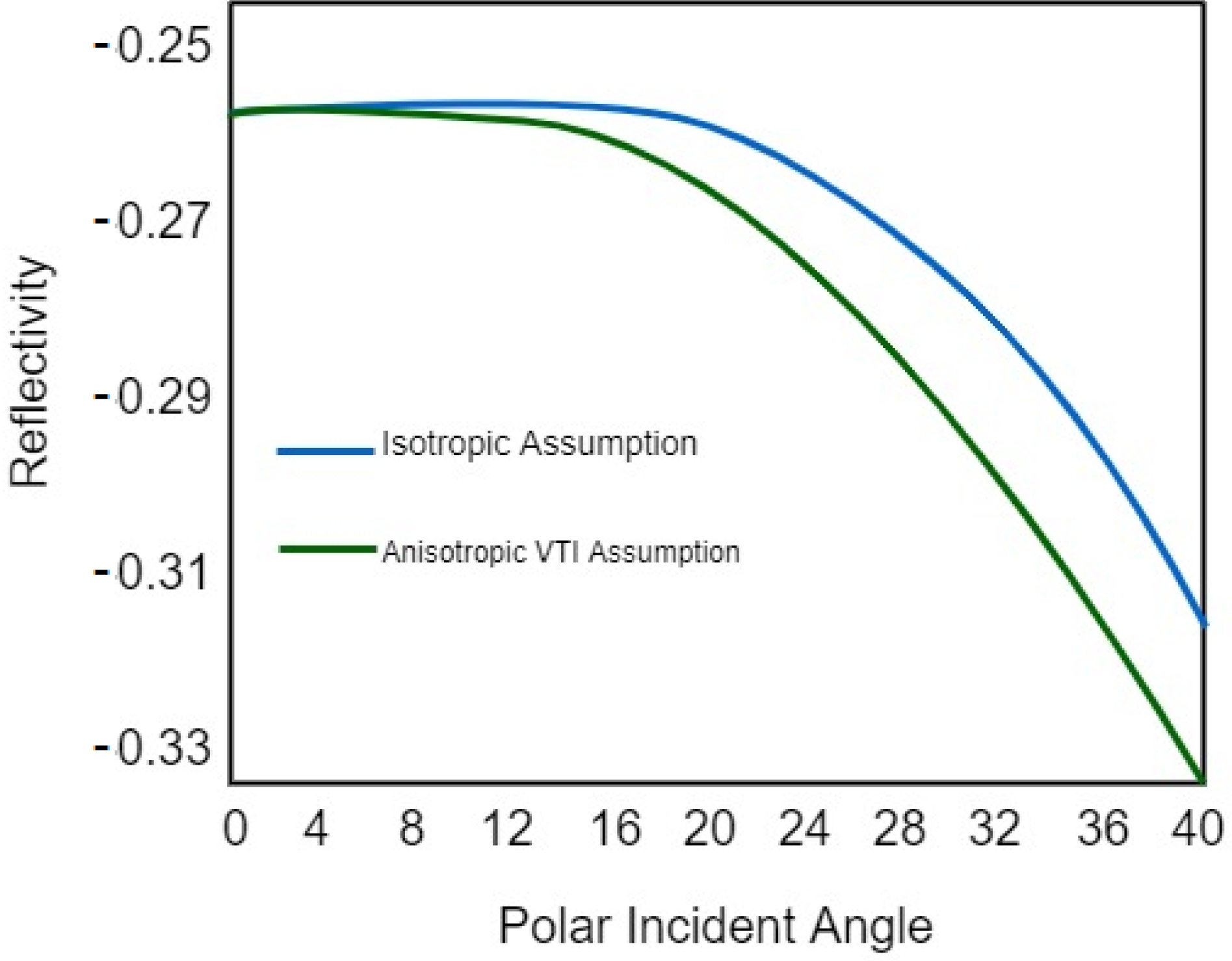
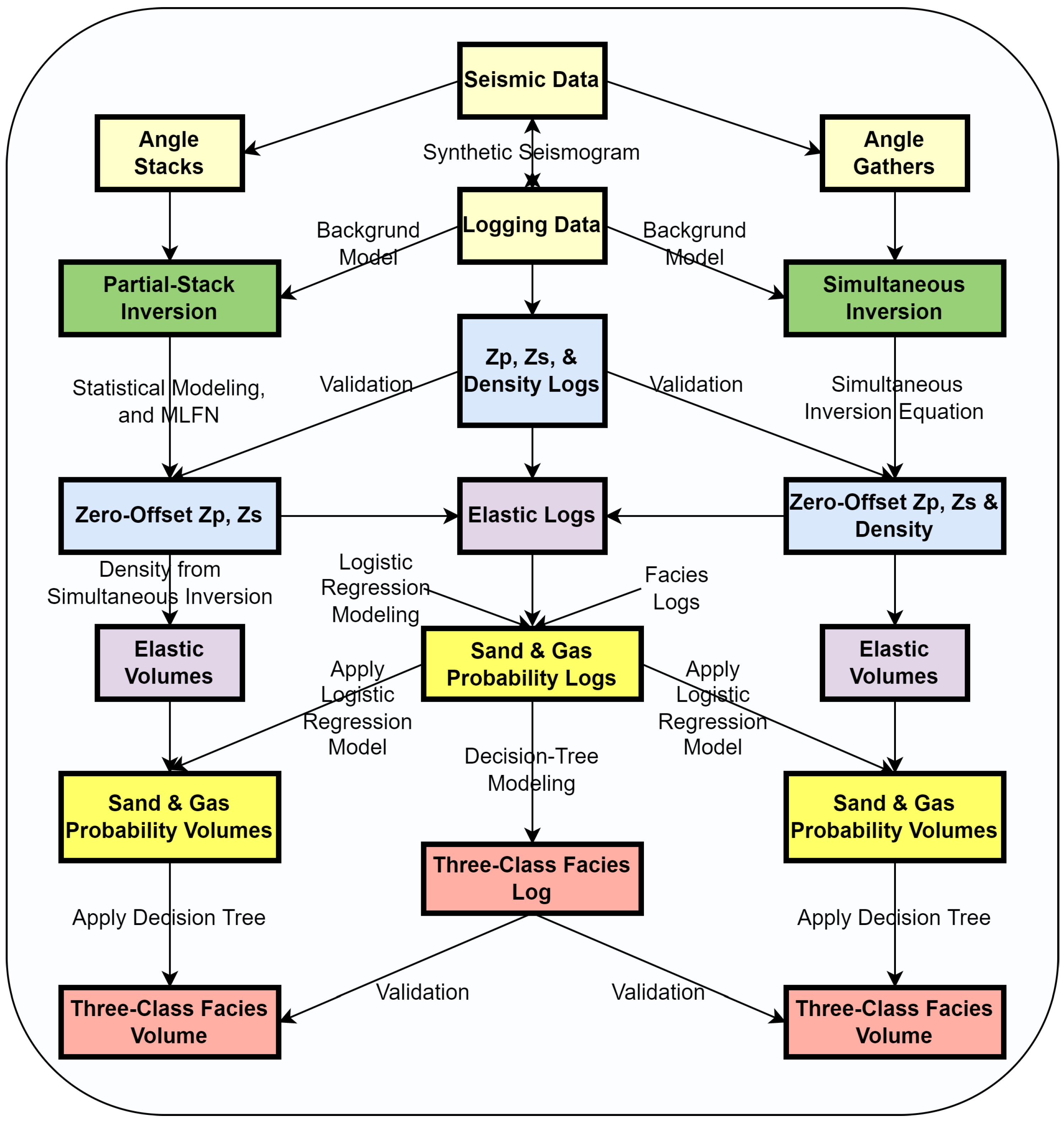
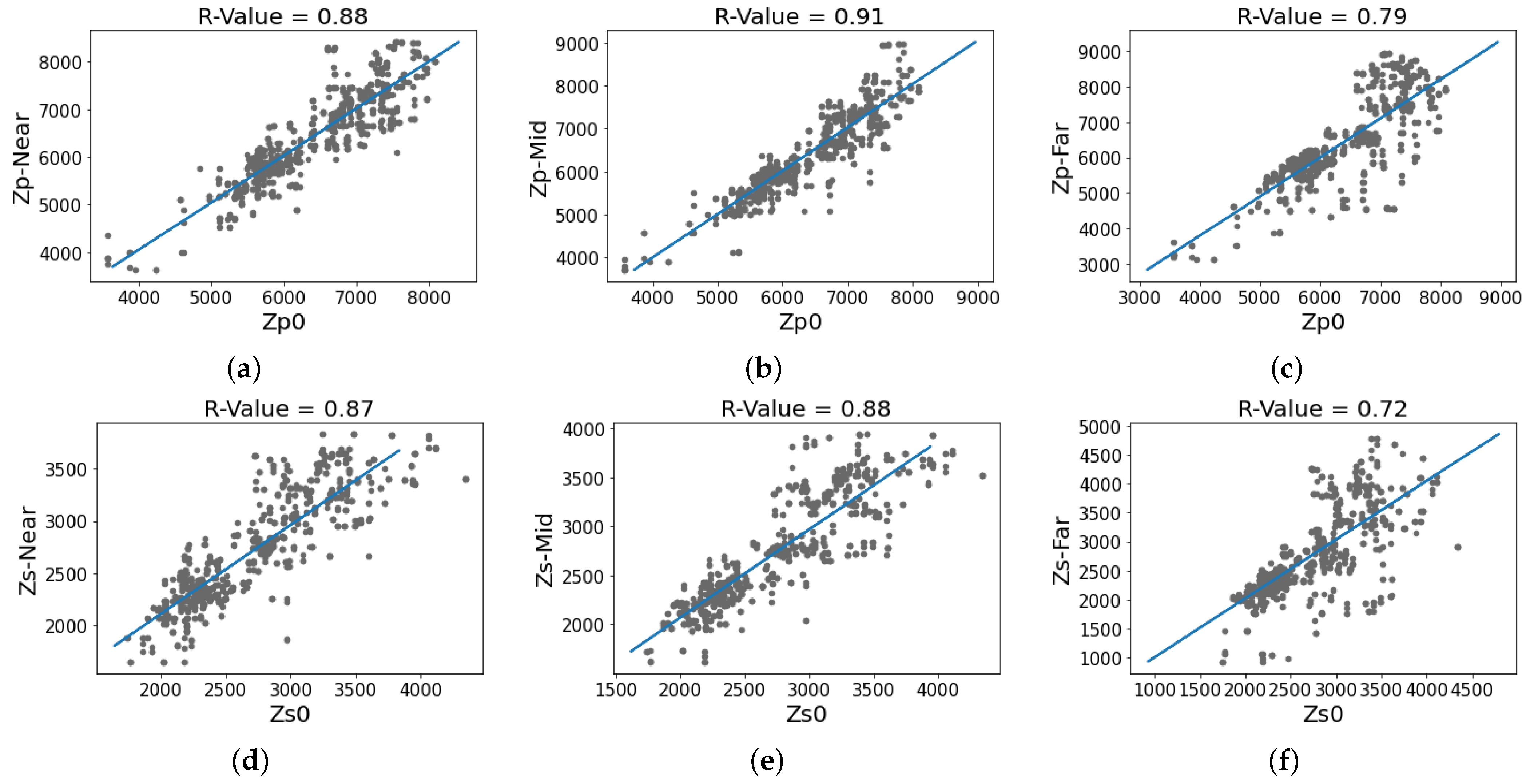
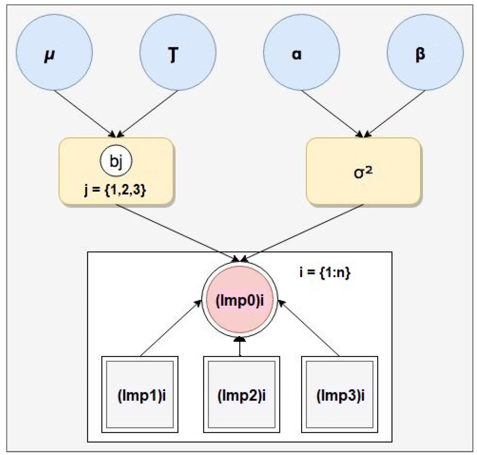
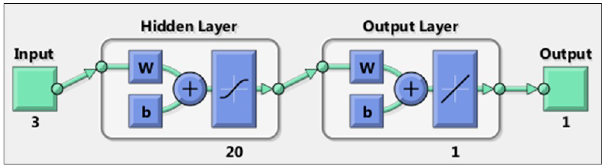
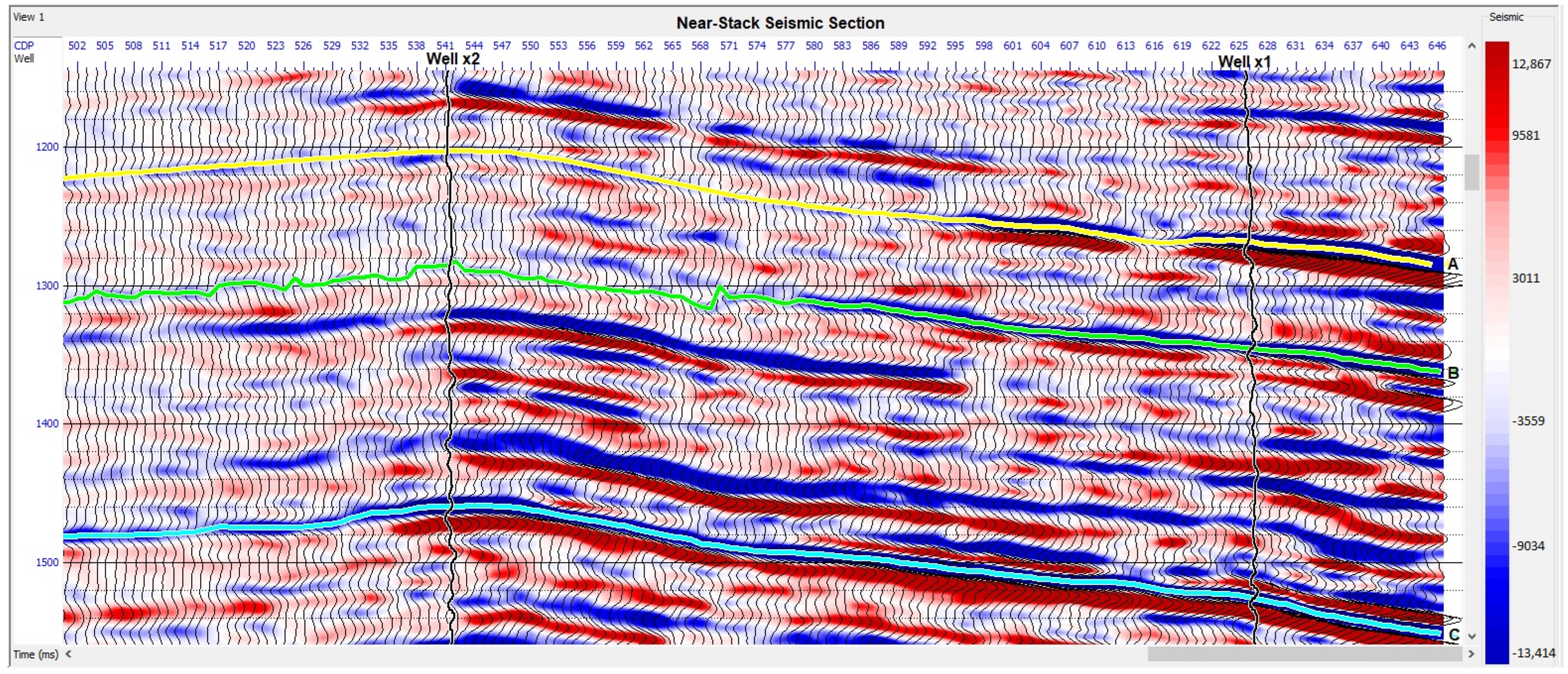
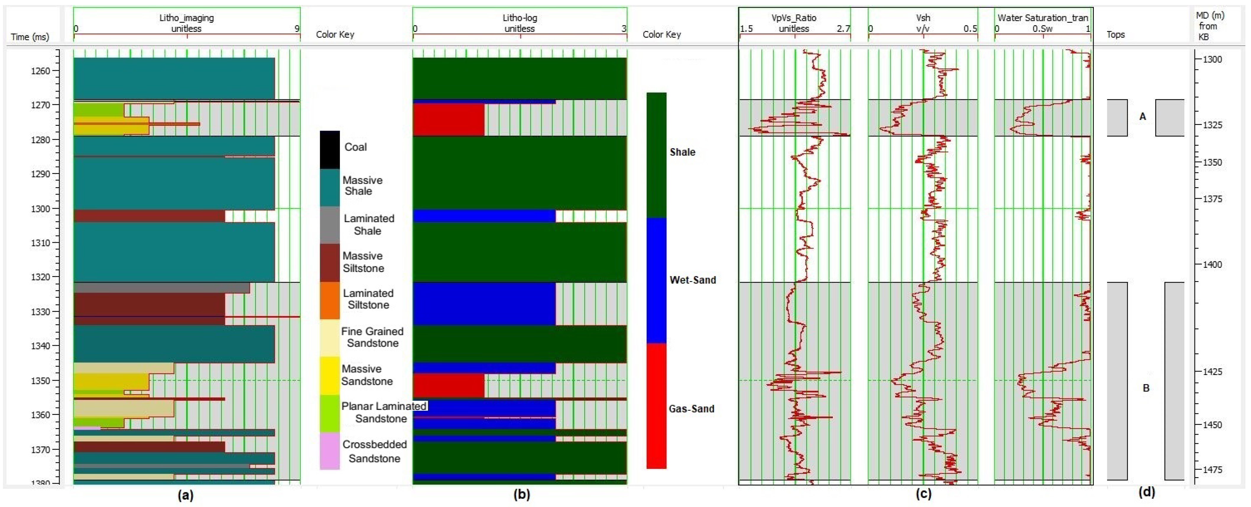
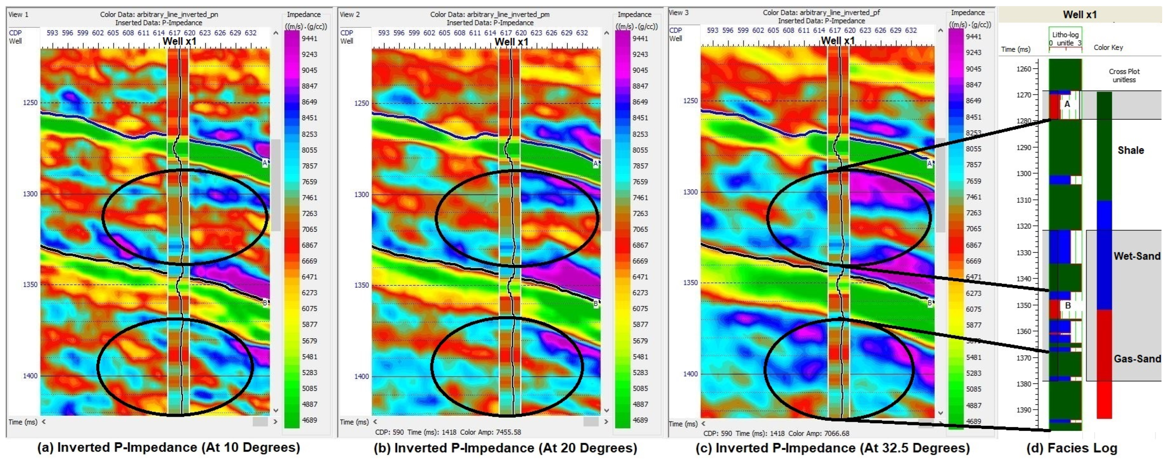
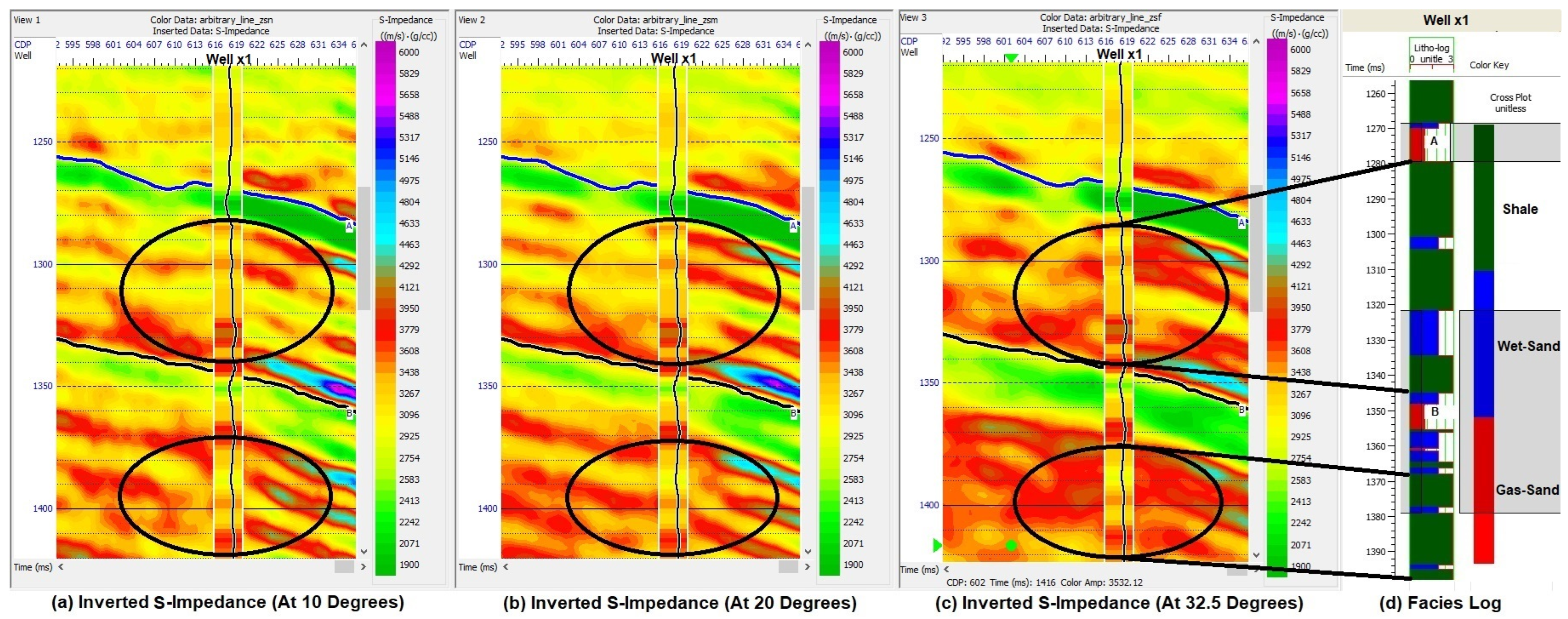
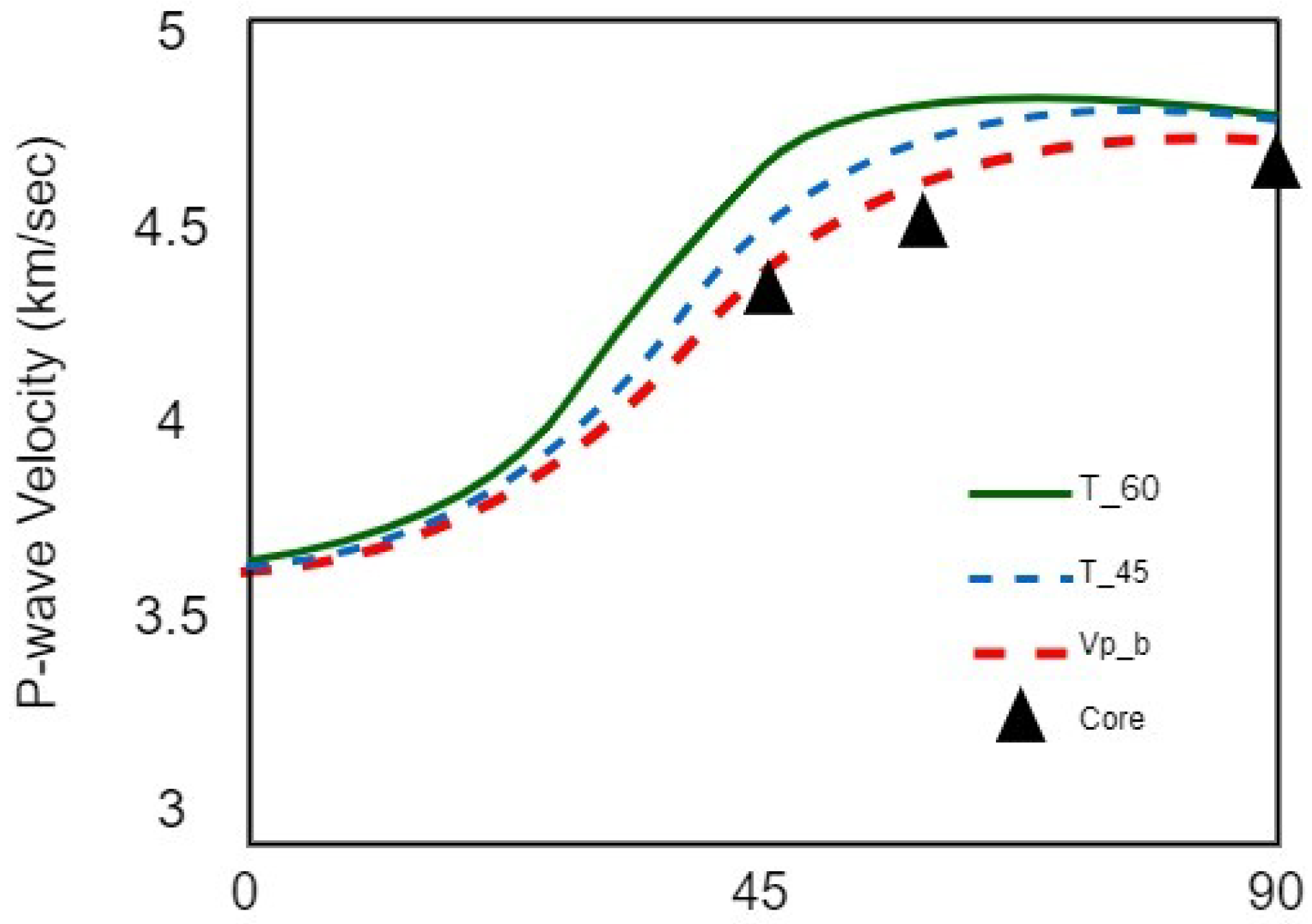
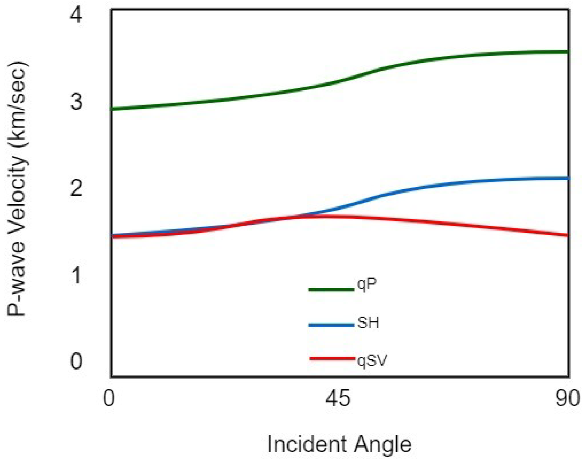
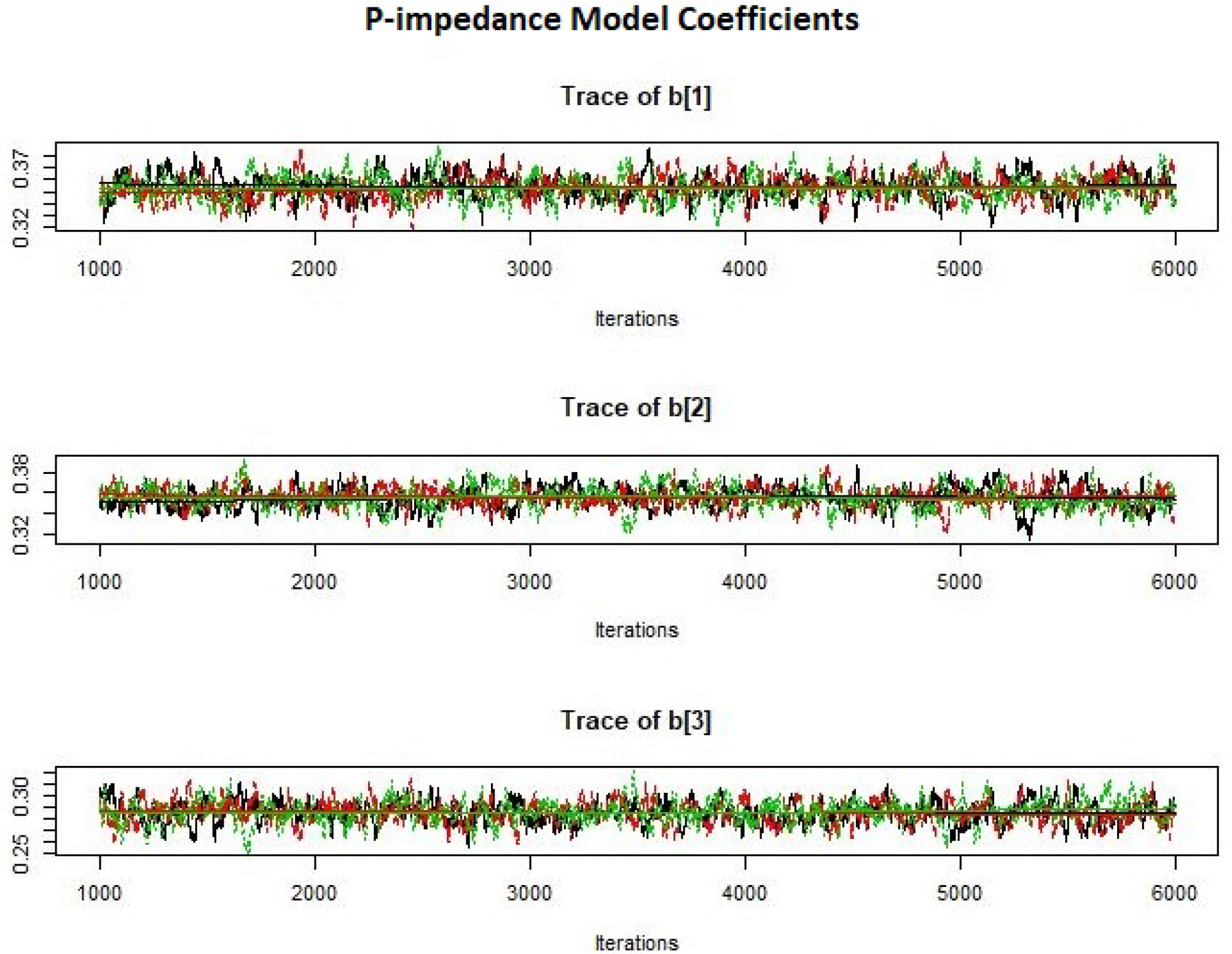
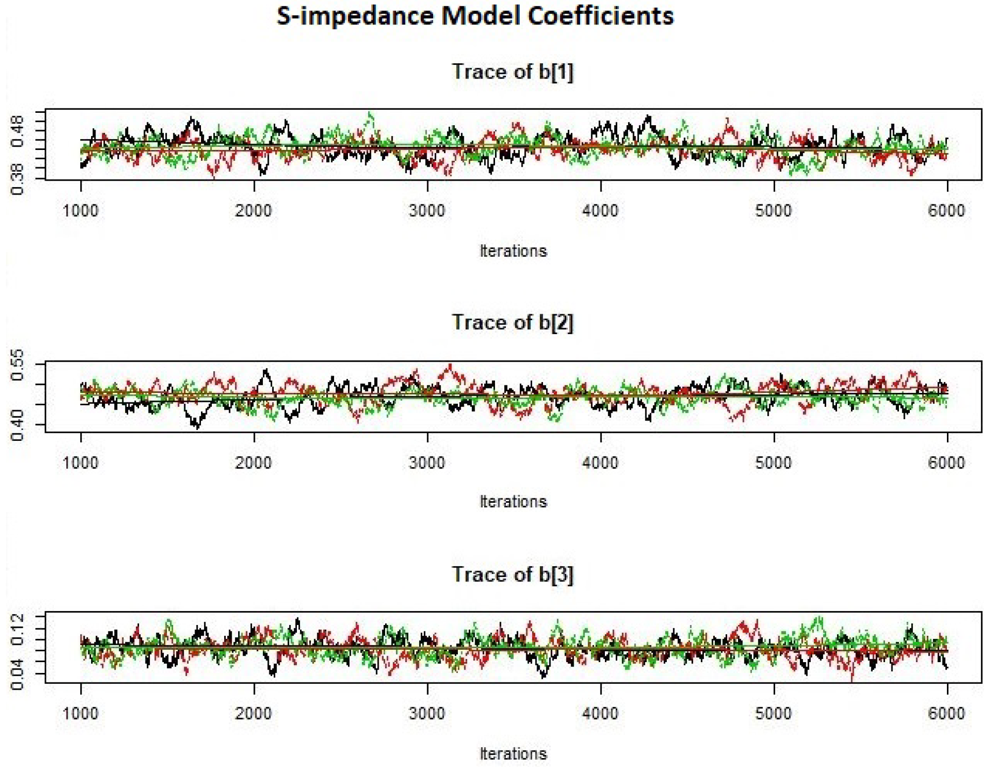
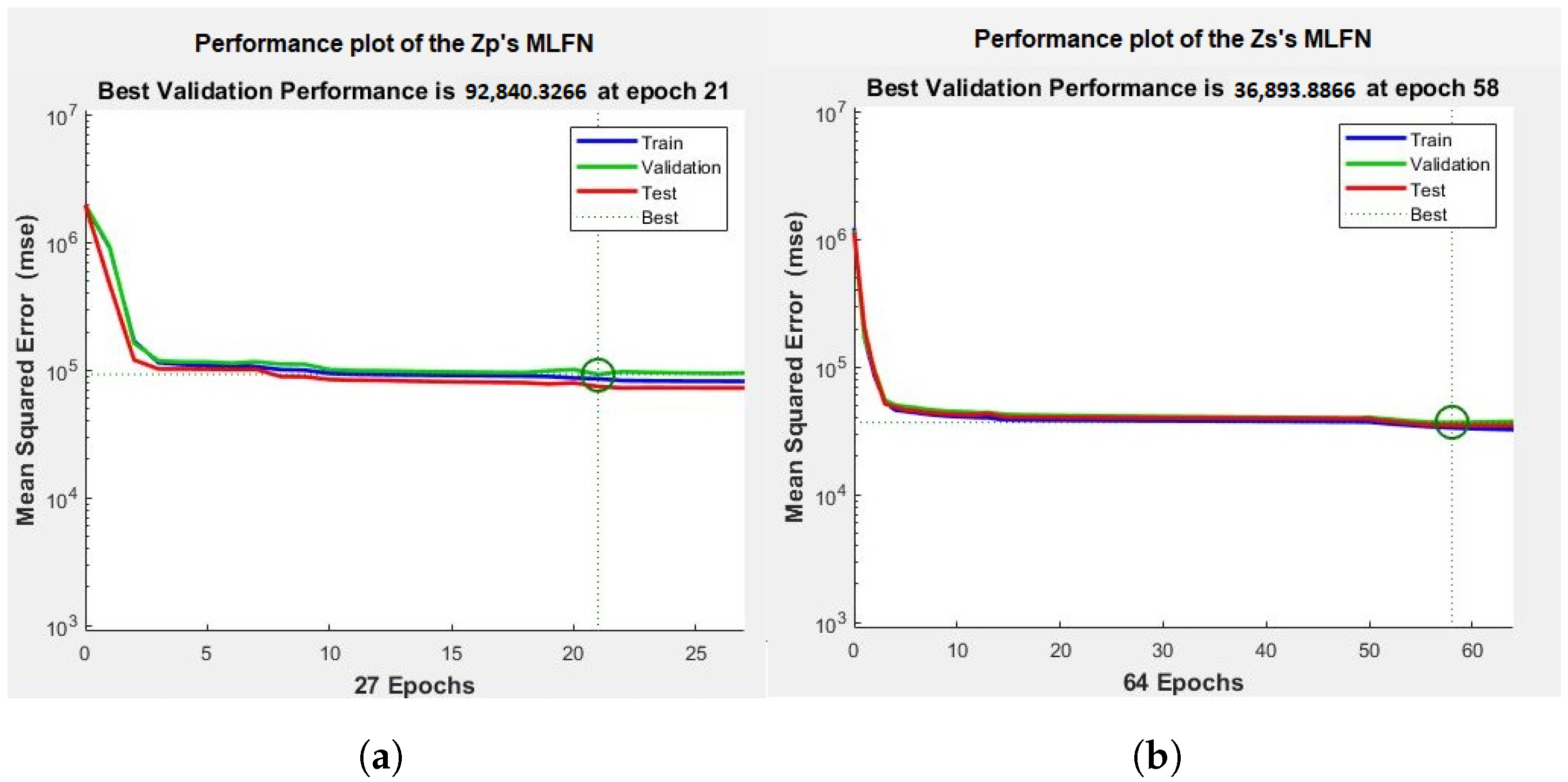
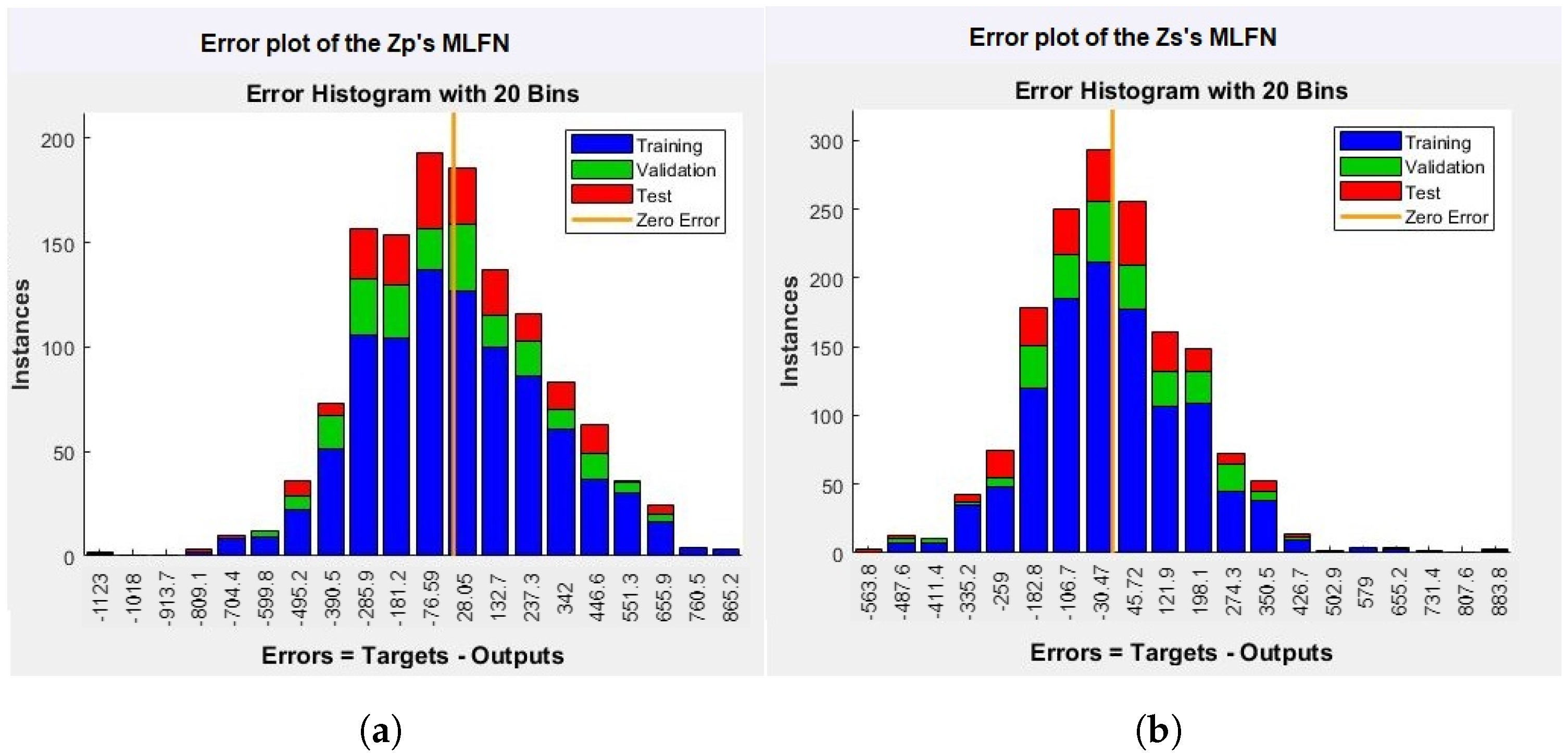
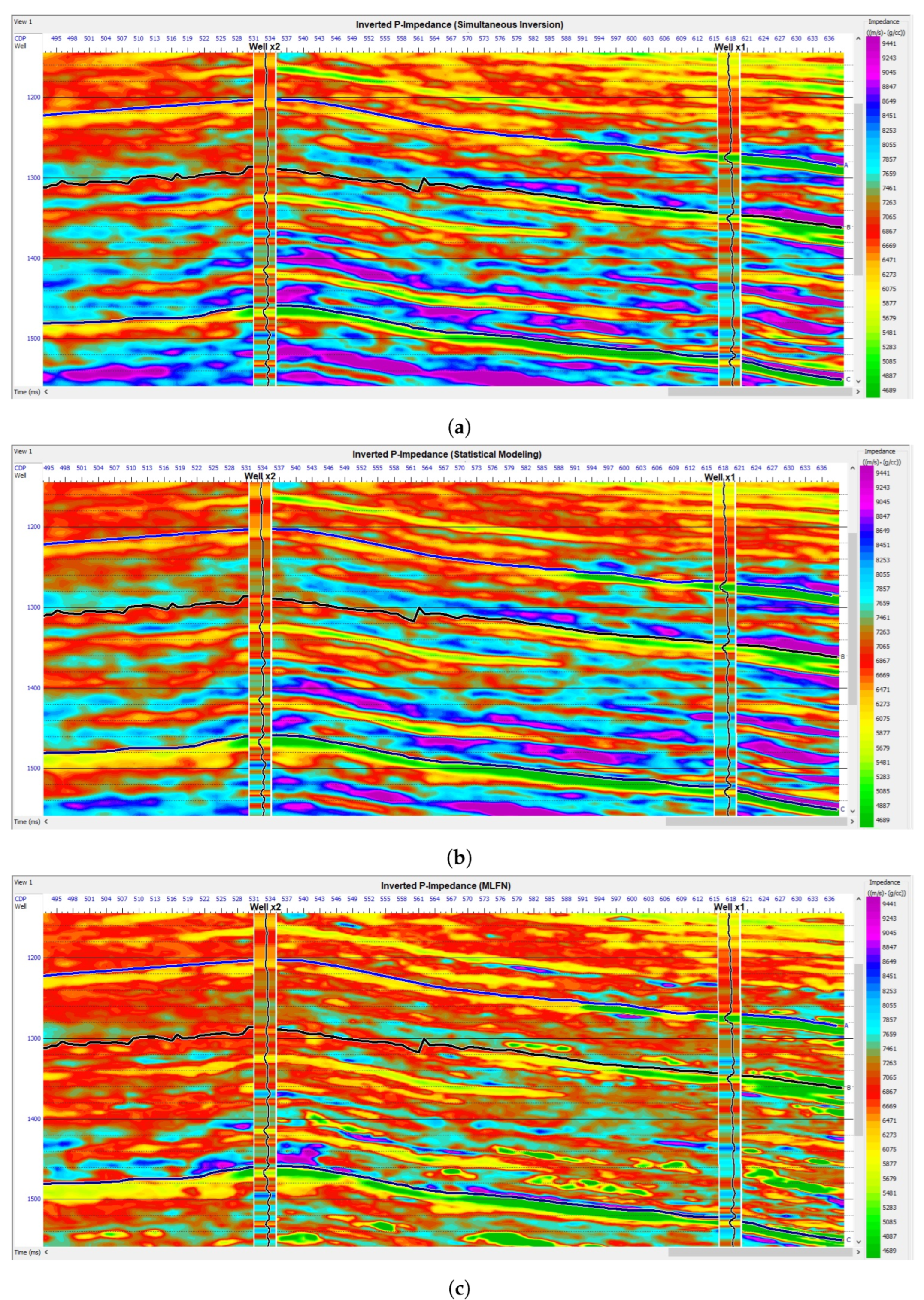
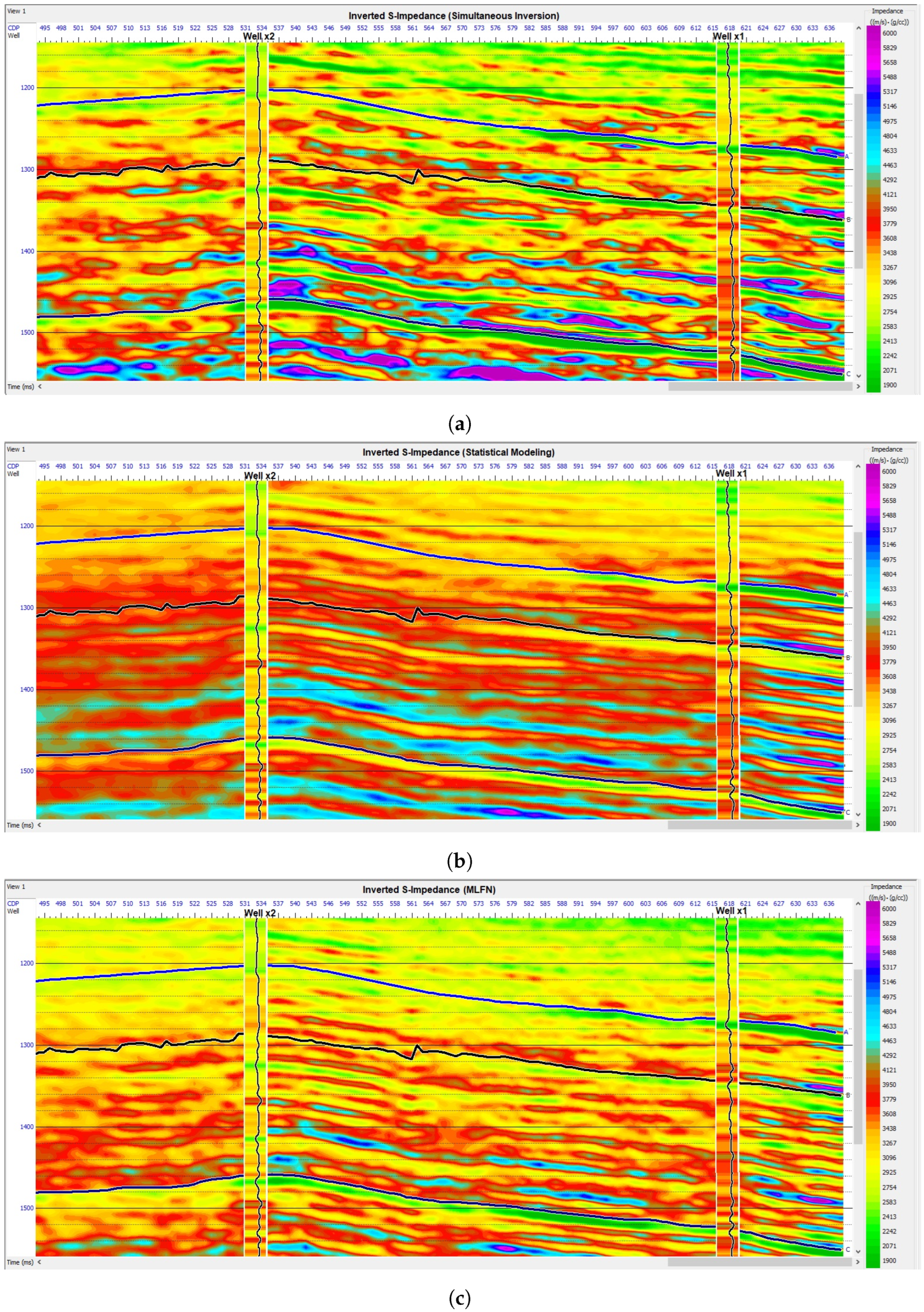
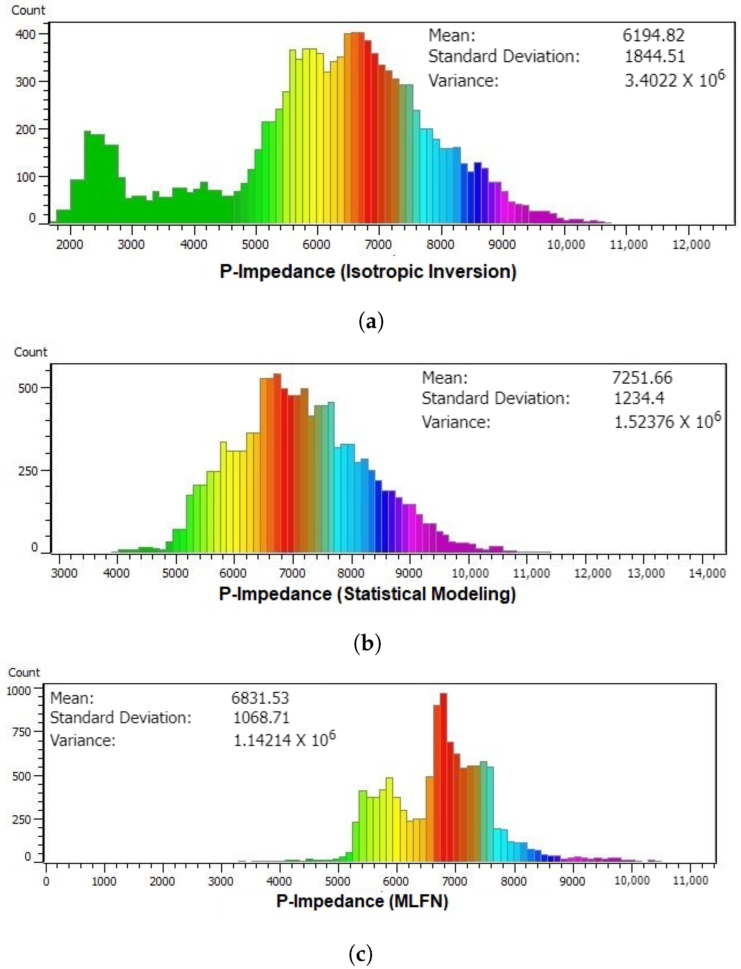
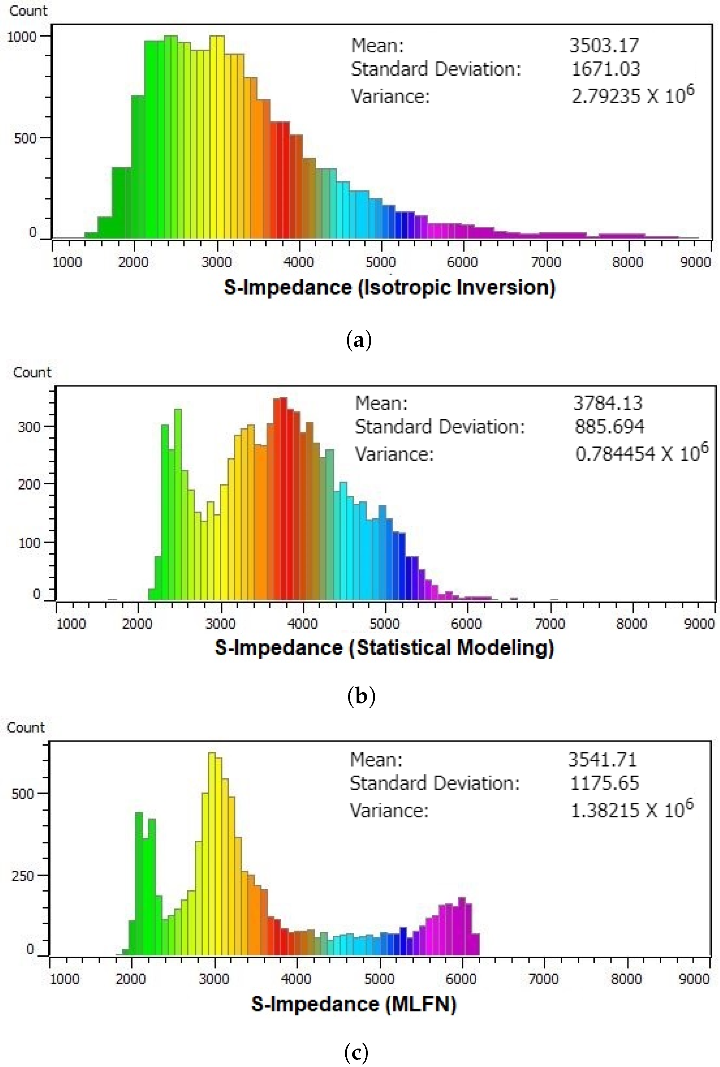
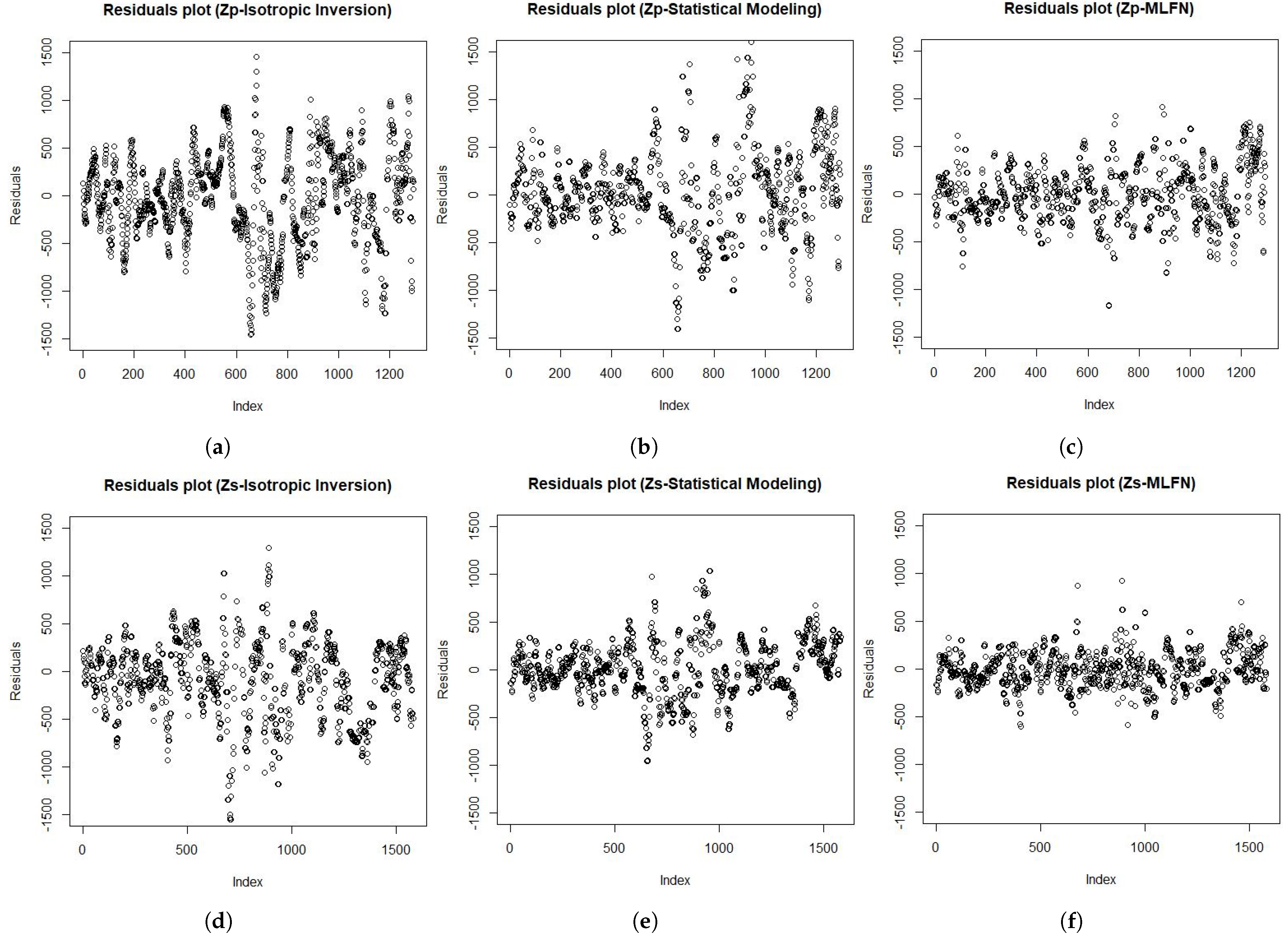
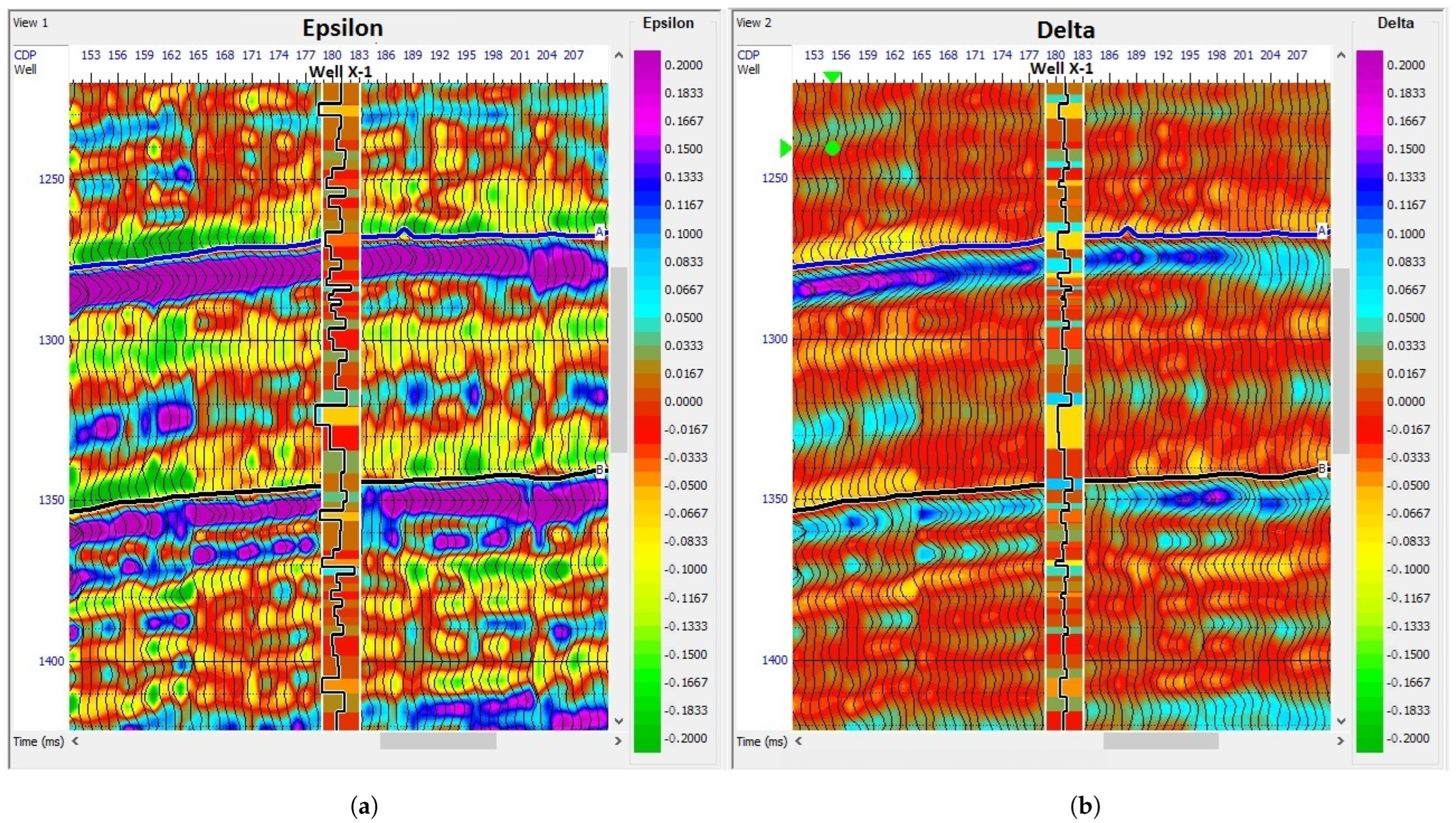
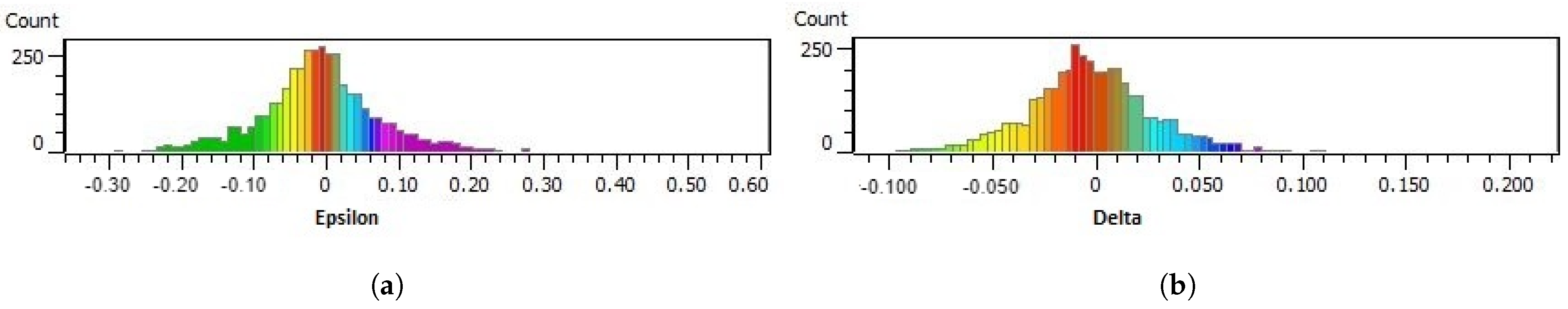
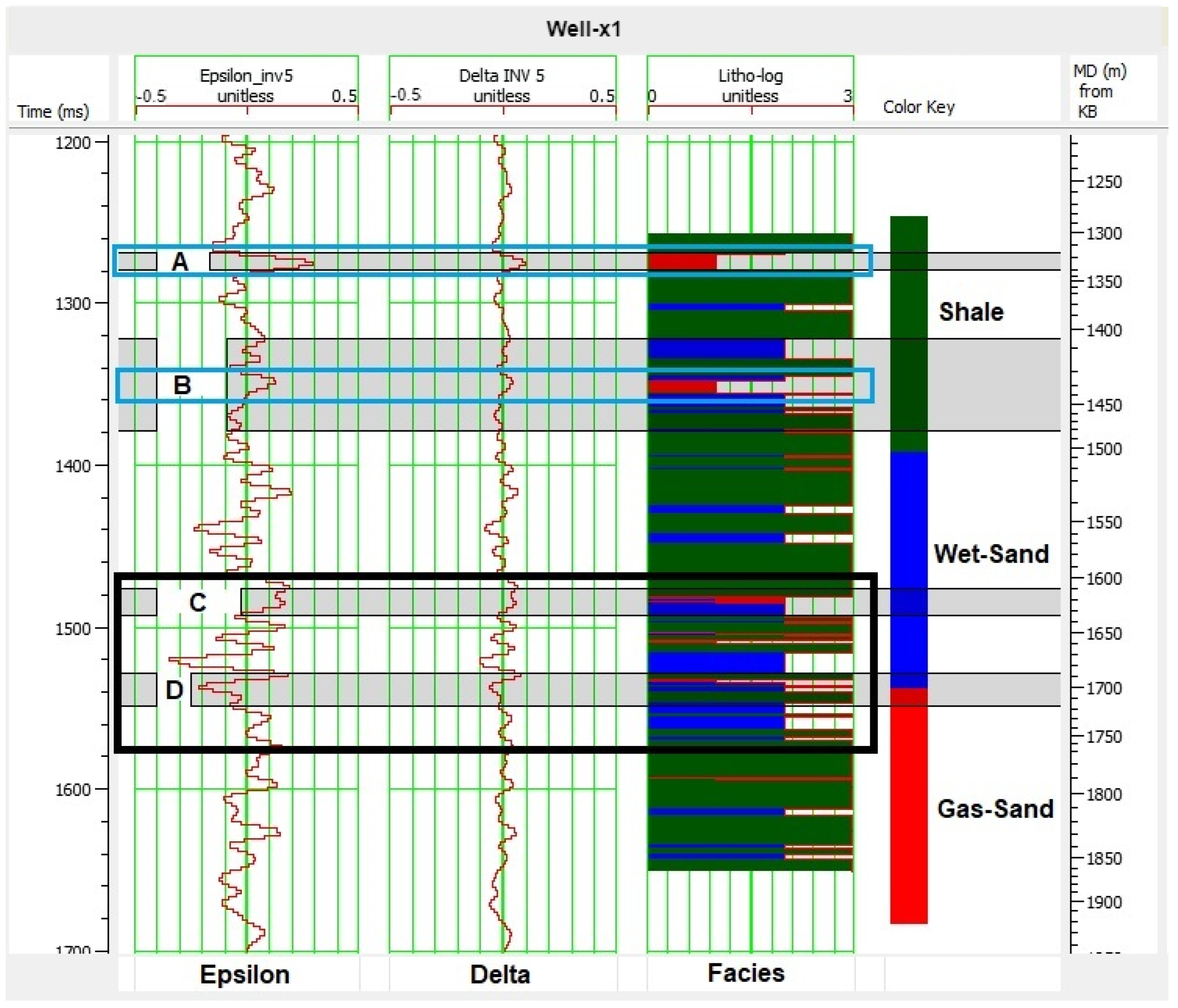
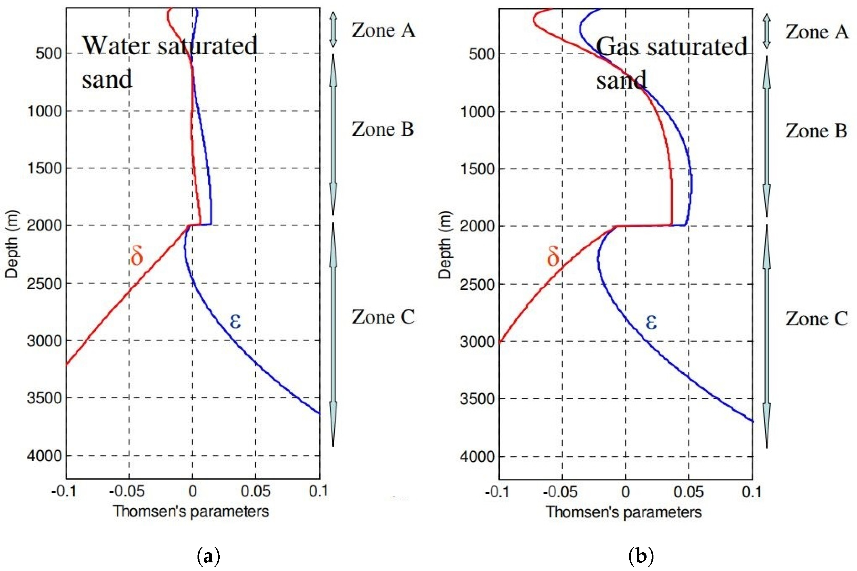
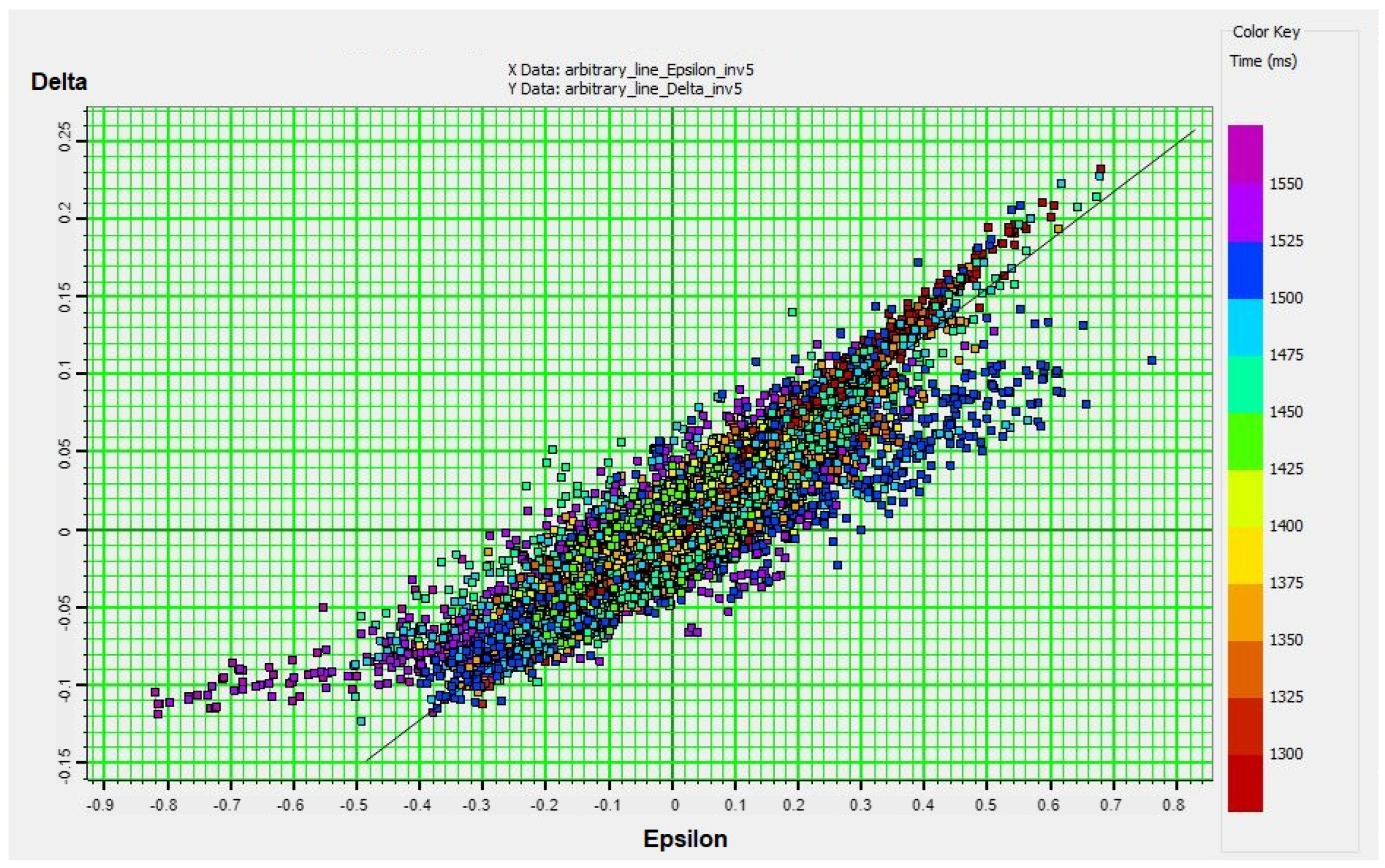
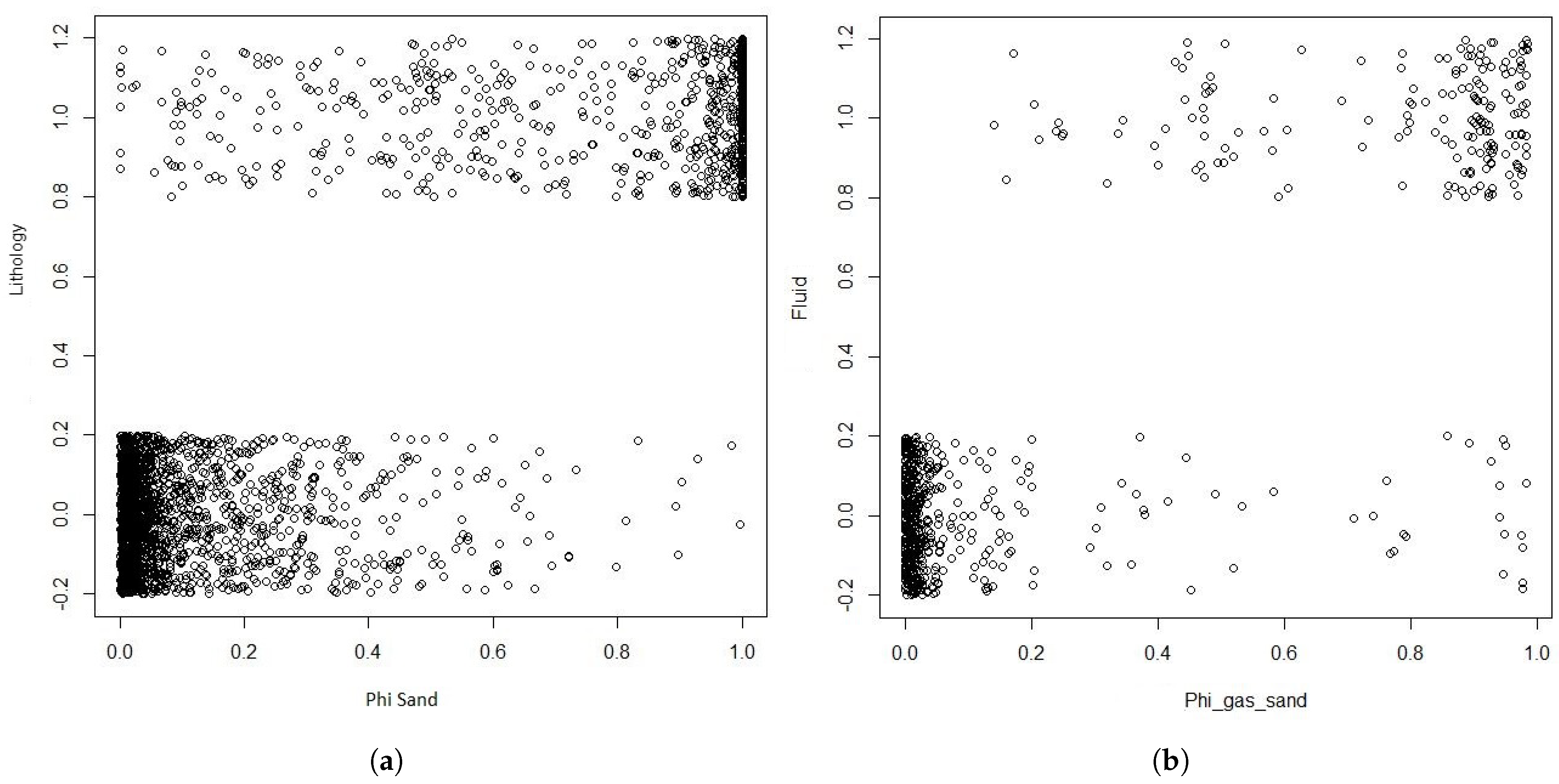
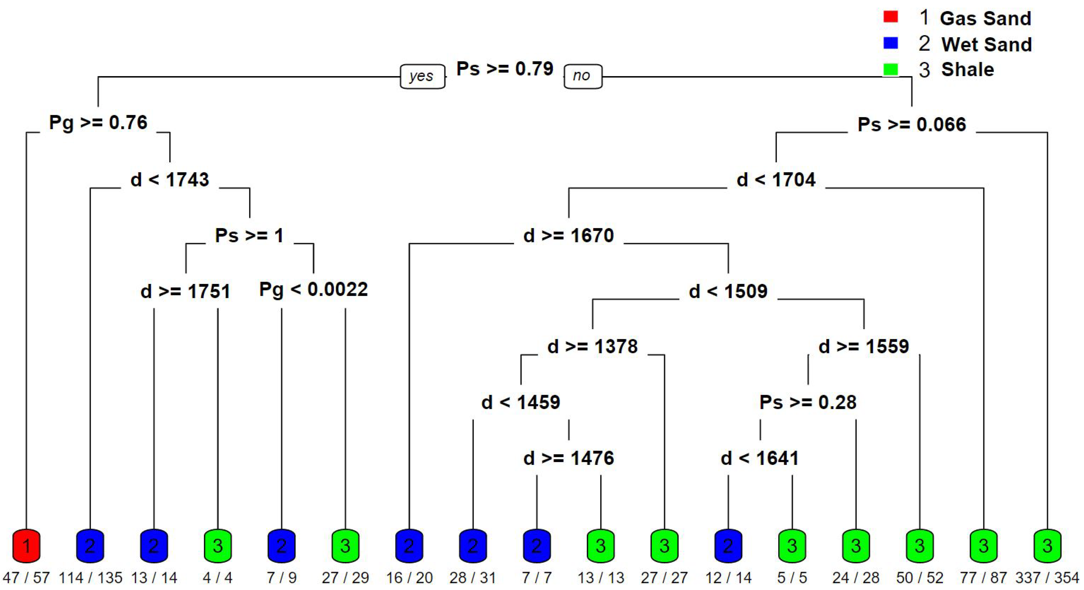
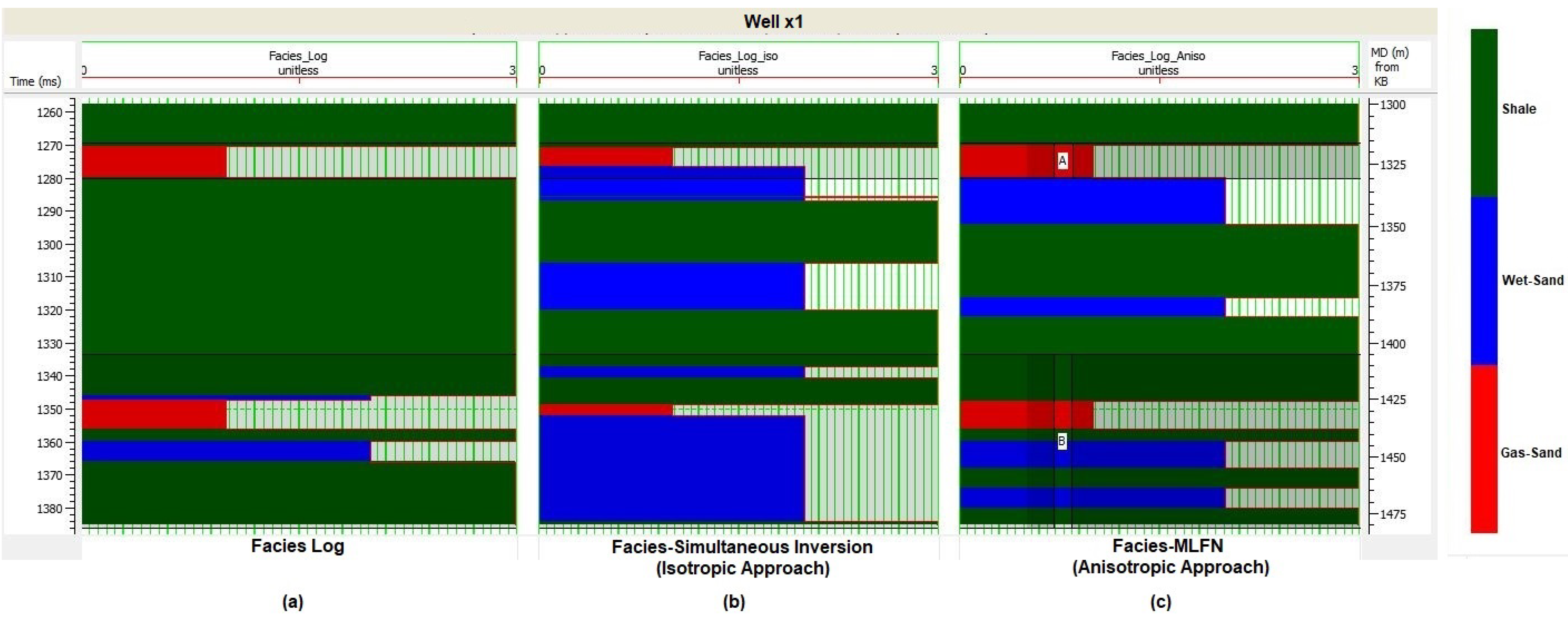
Table 1.
The statistical properties, mean (Mu) and standard deviation (SD), of the coefficients of the zero-offset and statistical models.
Table 1.
The statistical properties, mean (Mu) and standard deviation (SD), of the coefficients of the zero-offset and statistical models.
| Coefficient | ||||||
|---|---|---|---|---|---|---|
| Property | Mu | SD | Mu | SD | Mu | SD |
| Model | 0.3532 | 0.01 | 0.3555 | 0.01 | 0.286 | 0.01 |
| Model | 0.3672 | 0.01 | 0.364 | 0.01 | 0.266 | 0.01 |
Table 2.
The correlation coefficients of the predicted and obtained from isotropic inversion, statistical modeling, and MLFN at the wells (×1) and (×2).
Table 2.
The correlation coefficients of the predicted and obtained from isotropic inversion, statistical modeling, and MLFN at the wells (×1) and (×2).
| Property | Isotropic Inversion | Statistical Modeling | MLFN |
|---|---|---|---|
| 84% | 88% | 94% | |
| 73% | 85% | 92% |
Table 3.
The correct classification rates of the litho-fluid classes for isotropic inversion and MLFN.
Table 3.
The correct classification rates of the litho-fluid classes for isotropic inversion and MLFN.
| Method | Gas Sand | Wet Sand | Shale | All Facies |
|---|---|---|---|---|
| Isotropic Inversion | 51% | 82% | 55% | 56% |
| MLFN | 97% | 83% | 73% | 77% |
Publisher’s Note: MDPI stays neutral with regard to jurisdictional claims in published maps and institutional affiliations. |
© 2022 by the authors. Licensee MDPI, Basel, Switzerland. This article is an open access article distributed under the terms and conditions of the Creative Commons Attribution (CC BY) license (https://creativecommons.org/licenses/by/4.0/).
Share and Cite
MDPI and ACS Style
Gouda, M.F.; Abdul Latiff, A.H.; Moussavi Alashloo, S.Y. Estimation of Litho-Fluid Facies Distribution from Zero-Offset Acoustic and Shear Impedances. Appl. Sci. 2022, 12, 7754. https://0-doi-org.brum.beds.ac.uk/10.3390/app12157754
AMA Style
Gouda MF, Abdul Latiff AH, Moussavi Alashloo SY. Estimation of Litho-Fluid Facies Distribution from Zero-Offset Acoustic and Shear Impedances. Applied Sciences. 2022; 12(15):7754. https://0-doi-org.brum.beds.ac.uk/10.3390/app12157754
Chicago/Turabian StyleGouda, Mohammed Fathy, Abdul Halim Abdul Latiff, and Seyed Yasser Moussavi Alashloo. 2022. "Estimation of Litho-Fluid Facies Distribution from Zero-Offset Acoustic and Shear Impedances" Applied Sciences 12, no. 15: 7754. https://0-doi-org.brum.beds.ac.uk/10.3390/app12157754
Note that from the first issue of 2016, this journal uses article numbers instead of page numbers. See further details here.