

Reverse Time Migration Imaging Using SH Shear Wave Data
1
State Key Laboratory of Petroleum Resources and Prospecting, China University of Petroleum (Beijing), Beijing 102249, China
2
BGP Inc., China National Petroleum Corporation, Beijing 100083, China
*
Author to whom correspondence should be addressed.
Appl. Sci. 2022, 12(19), 9944; https://0-doi-org.brum.beds.ac.uk/10.3390/app12199944
Submission received: 9 August 2022
/
Revised: 29 September 2022
/
Accepted: 30 September 2022
/
Published: 3 October 2022
(This article belongs to the Special Issue Technological Advances in Seismic Data Processing and Imaging)
Abstract
:Featured Application
Imaging through gas clouds using SH shear wave.
Abstract
In this paper, we discussed the reverse time migration imaging of compressional wave (P-wave) and horizontally polarized shear wave (SH shear wave) seismic data, together with P- and SH shear wave constrained velocity model building. In the Sanhu area in Qaidam Basin, there are large areas of gas clouds, which leads to poor P-wave seismic imaging. The P and SH shear wave seismic data of a co-located survey line with the same acquisition geometry were used to access their imaging capability using reverse time migration. We first estimated the change in P-wave and SH shear wave velocity ratio using pre-stack time migration (PSTM) for constraining the overall depth domain velocity model. Additionally, we then used an eighth-order finite difference scheme for P-wave reverse time migration on a variable grid and used the sixth-order combined compact difference (CCD) wave field simulation method for SH shear wave reverse time migration on a regular grid. The results show that the constrained velocity model produces a good match in the overall geological structure shown in the P-wave and SH shear wave reverse time migration results. However, in the gas cloud areas, SH shear wave reverse time migration has obvious imaging advantages, which can clearly image the structure inside the gas clouds.
1. Introduction
Currently, the main means of oil-gas exploration are mainly based on the P-wave (compressional wave). A series of mature technologies developed for P-wave exploration, including data acquisition, data pre-processing, pre-stack time migration, and pre-stack depth migration, have made great progress and are still making progress. However, with the extension of exploration to low permeability, deep and unconventional reservoirs and the increasingly complex exploration targets, relying solely on P-wave technology is facing more and more challenges. Through an analysis of the limitations of P-wave exploration and the potential of shear wave exploration, Gou et al. [1] proposed the effectiveness and applicability of SH shear wave (horizontally polarized shear wave) exploration technology and conducted SH shear wave data acquisition and processing tests in an exploration area in Western China [2].
Generally speaking, the resolution of seismic exploration is a quarter of the wavelength, which depends on the velocity and frequency. As the wave velocity of subsurface media is objective and certain, the resolution can only be improved by increasing the frequency. In terms of tight reservoirs or deep carbonate reservoirs, the P-wave velocity can be higher than 5000 m/s, and the effective frequency will be reduced to about 30 Hz with the attenuation of deep high-frequency components, which is very unfavorable for the identification of deep thin layers [3,4]. The further improvement of the effective frequency band in the deep layer will face great challenges in source excitation. If the frequency band is consistent, the wave speed of the shear wave is usually about half that of the P-wave, and the resolution can reach twice that of the P-wave. Shear-wave exploration is one of the effective ways to improve the resolution [5,6,7].
In recent years, with the rapid development of computer calculation, reverse time migration has gradually become an industrial applied imaging technology used to solve the imaging of various complex structures. Compared with that of the P-wave, the shear wave velocity is low and the frequency band is wide, such as carbonate rocks (Takougang et al., 2020) [8], which can improve the resolution of the formation; the shear wave propagation is only related to the rock frame, which can be used to accurately construct the subsurface structure. In terms of the near offset, the shear wave has a higher signal-to-noise ratio than the P-wave, so it has higher inversion precision [9,10,11,12,13,14,15,16]. To improve the accuracy and efficiency of shear-wave pre-stack depth migration, it is necessary to apply a high-precision finite-difference scheme to shear wave seismic imaging on the basis of the low-speed characteristics of the shear wave, and this method needs to maintain good accuracy of spatial difference and time difference under the condition of a large spatial grid and time step. Thus, migration algorithm selection is one of the subjects discussed in this paper.
Since the mid-1990s, reverse time migration has been applied to multi-component wave seismic data excited from an elastic-wave source [17,18,19,20], and it has overcome calculation problems and interference artifacts in P- and shear wave simulation. In recent years, most studies have focused on the P- and shear wave decoupled method to separate P- and shear waves [21,22,23,24,25,26,27,28]. In these studies, there is no case of the direct use of shear wave data for reverse time migration, but the elastic wave field was used to separate P- and shear waves or decoupled P- and shear wave fields obtained from the elastic-wave equation. This paper will focus on the direct use of SH shear wave source data for reverse time migration imaging and together with corresponding procedures for velocity analysis and velocity model building.
The study area, Sanhu, referred to in this paper, is located in the Qaidam Basin. The reservoir in the area is mainly consisted of thin sand-mudstone interbed and unconsolidated sandstone reservoirs, and this area is the largest Quaternary biogas production area discovered in China. Affected by the reservoir gas, the reservoir imaging is seriously blurred and distorted. To determine the characteristics of the study area, in this paper, the SH shear wave velocity model in the depth domain is established by using the SH shear wave data in the survey, and the subsurface reflecting interface in this area is imaged by using the SH shear wave reverse time migration imaging technology [29,30]. During depth domain velocity model building, we obtain the P-to-SH shear wave velocity ratio in the area from the time domain P-wave and SH shear wave imaging results, which is used to constrain the overall P- and SH shear wave depth domain velocity model building.
2. Application Background and Method Principles
2.1. Survey Background
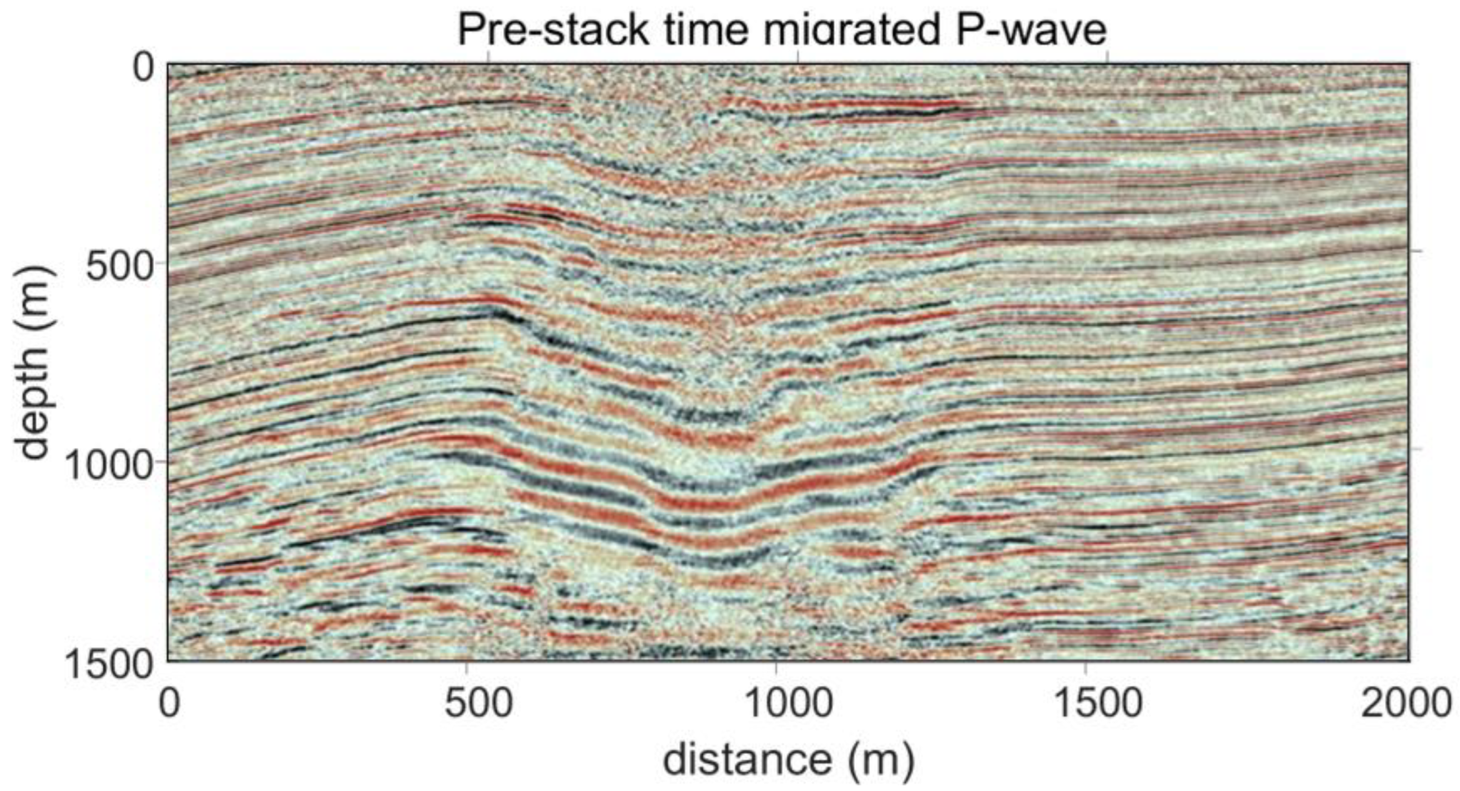
The survey studied in this paper is from the Sanhu area of the Qaidam Basin, and its surface is mostly composed of aeolian monadnock, sand dunes, sandbag, saline-alkali land, hard-alkali land, salt marsh, etc. The Sanhu area is a biogas enrichment area. Affected by subsurface gas, as shown in Figure 1 the energy and frequency absorption of P-wave seismic data in the seismic anomaly area is serious, the data signal-to-noise ratio is low, and the structure is distorted [31]. It is difficult to obtain reliable imaging of low-relief structures.
At the same time, there are unique geological characteristics of the Quaternary system in the Sanhu area, such as weak diagenesis, a thin sand-mudstone interbed, an indiscriminate hydrocarbon source and reservoir, as well as the succession and relay of gas generation. Under this unique geological background, a high resolution is required for imaging the structure in this area, and SH shear wave imaging has a high stratigraphic resolution due to its low velocity and wide frequency band.
2.2. Principle of Reverse Time Migration
The principle of SH shear wave reverse time migration (RTM) used in this paper is briefly introduced below:
Reverse time migration based on the solution of two-way wave equation is the most advanced pre-stack depth migration imaging. After an accurate velocity model is obtained, SH shear wave reverse time migration imaging (SH-RTM) generally includes three steps [32]:
- (1)
- The source wave field is obtained by using the source constructed manually or extracted from actual data, and the corresponding model is numerically simulated to obtain the source wave field , where is the space vector.
- (2)
- Using the seismic data obtained at the receiver, the reverse continuation propagation passes through the same velocity model, and the corresponding receiver wave field is obtained, where the position of the receiver is .
- (3)
- We can then apply appropriate imaging conditions, such as cross-correlation, we obtain the (reverse-time migration image results):where is the source wavefield obtained by forward modeling, is the receiver wavefield obtained by reverse continuation simulation at the same time under the same velocity model, and t is the total propagation time.
It can be seen from Equation (1) that the final result of reverse time migration is affected by the accuracy of the source wave field and the receiver wave field . Therefore, in order to obtain accurate imaging of the target area, it is necessary to make good use of high-quality SH shear wave data and apply them to reverse time migration.
2.3. Depth Domain Velocity Model Building for SH Shear Wave Data
The depth domain velocity model building is very important for the effect of depth domain imaging, and P-wave and SH shear wave data are simultaneously acquired in this study area [33]. In depth-domain imaging, the reflector of the subsurface structure, the P-wave and SH shear wave, should be matched [34]. Generally, in the case of the combination of shear wave or converted wave and P-wave imaging, a priority will be given to determine the P-wave velocity (VP) during the model establishment, and then a P-to-S wave velocity ratio will be estimated and used together with the VP (P-wave velocity) to establish the model of SH shear wave velocity (VS). In this study area, due to the gas clouds and the difficulty of obtaining effective signals of P-waves, it is difficult to establish a velocity model of VP. While the pure SH shear wave can propagate through the rock frame without being affected by gas and fluid, the pure SH shear wave data can be directly used to establish a model of the SH shear wave velocity vs. (SH shear wave velocity).
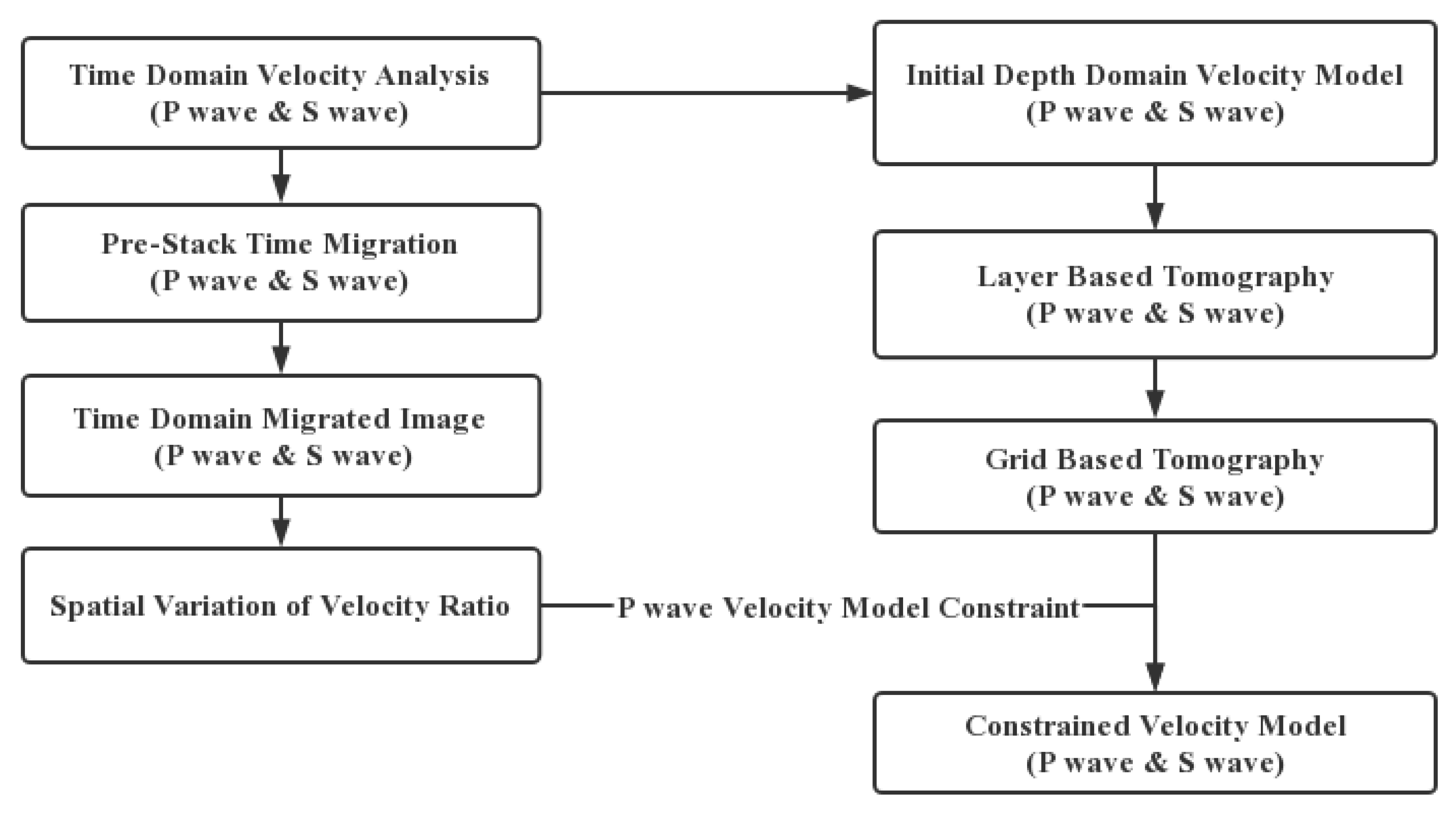
First of all, we separately used the SH shear wave and P-wave velocity models. The establishment of P-wave velocity model refers to the establishment of SH shear wave velocity model since SH shear wave data in the region has a better signal-to-noise ratio in the survey and is more credible in the absorption area. Then, the velocity ratios of the P- and SH shear waves in this region are estimated, and the obtained ratios are taken as constraints. In order to better match the imaging of the P-wave and SH shear wave in the depth domain, we also need to estimate the change in the velocity ratio of the P-wave and SH shear wave by using the pre-stack time migration image. There are many methods of depth domain velocity model building, and we mainly use layer- and grid-based tomography. After the establishment of the two models, the spatial P-wave-to-SH shear wave ratio mentioned above is used to obtain the interlayer travel time in the depth domain model, calculate the proportion of model correction, and apply it to the correction of the P-wave model. In the actual constraint process, the velocity correction is about 1–3%, which can be attributed to weak anisotropic media.
2.4. Principle of Combined Compact Difference Scheme
The combined compact difference (CCD) to suppress the numerical dispersion caused by the spatial step size are enclosed in this paper to solve the problem of low SH shear wave velocity; the formula is as follows [35,36]:
In Equation (2), is the grid spacing, are the difference coefficient matrices; f is the function value of node ; and represent the first- and second-order derivatives of node , respectively; represent the function values of node successively m nodes forward and m nodes backward; represent the first-order derivatives of node successively one node forward and one node backward, respectively; represent the second derivative of node one node forward and one node backward. The wave field of the SH shear wave can be simulated with the above method applied to the numerical simulation of SH shear wave propagation under the condition of a two-dimensional medium.
In this paper, we use the three-point sixth order format of Equation (2) for the SH shear wave reverse time migration, that is, Formula (3).
3. Analysis of Combined Compact Difference Scheme
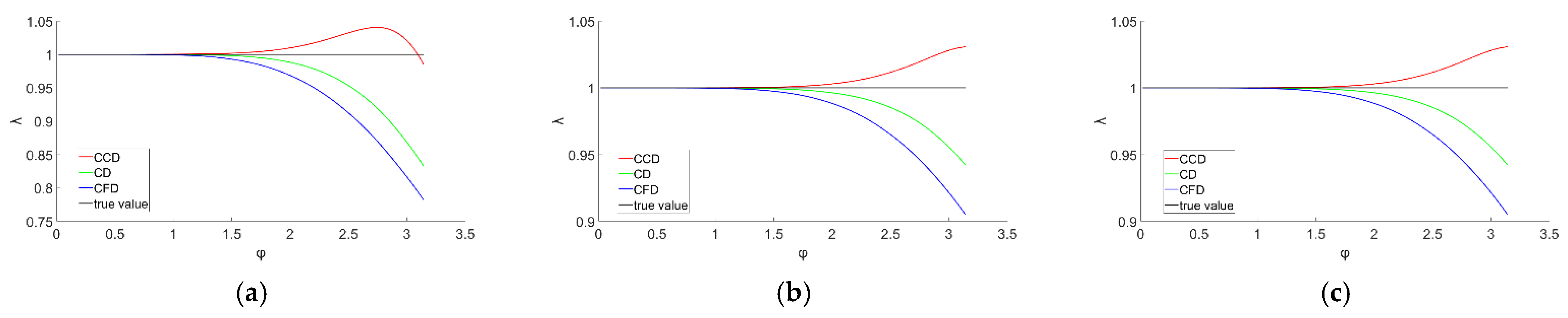
In numerical simulations, if the size of the spatial grid is too large, it will cause large solution errors and produce numerical dispersion [37,38]. The simple harmonic wave solution is introduced to have the velocity ratio curve at different values in the isotropic case; is the angle between the wave’s propagation direction and the x-axis. It is used to compare the spatial dispersion suppression effects of CCD with the traditional finite difference scheme. It is shown as follows:
In Figure 2, the ratio of numerical wave velocity to true velocity is defined as:
where is the numerical wave velocity, and is the true wave velocity. It is shown in Figure 2 that with the velocity ratio curves of the CCD, the other two different formats at different values. The Courant numbers () are 0.25, the horizontal axis is the product of the wavenumber and the spatial step, and the y-coordinate is the velocity ratio , with 1 meaning that the numerical wave speed is consistent with the theoretical wave speed and indicating that the numerical dispersion is low. It also indicates that CCD has the best suppression effects.
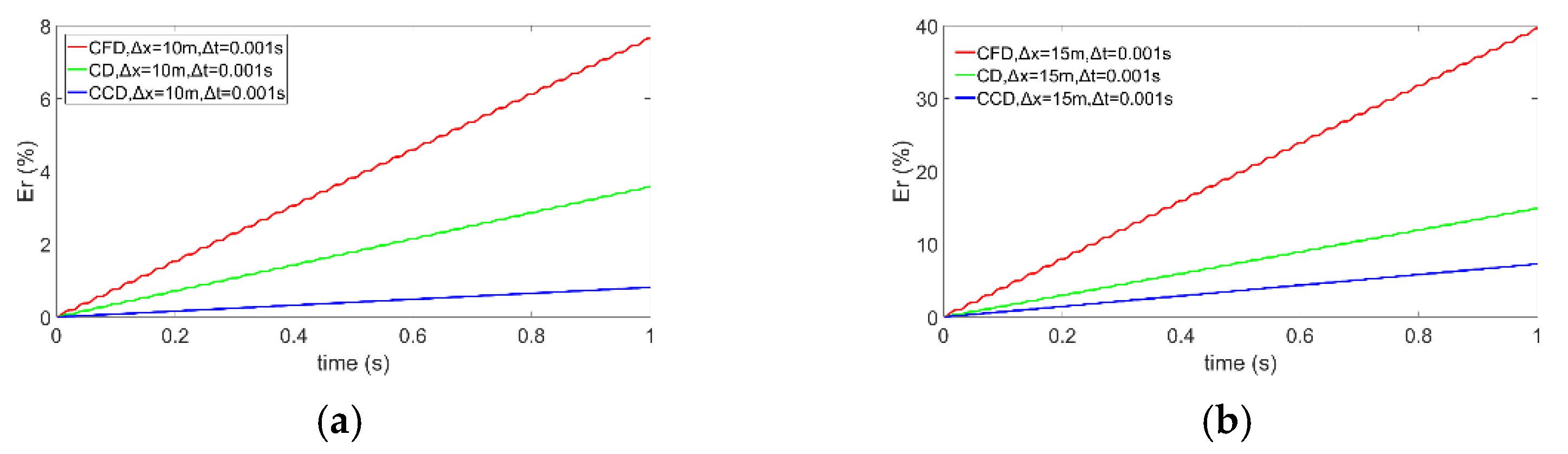
Additionally, the simulation error is calculated by simulating the two-dimensional plane harmonic initial value problem to analyze and compare the numerical simulation accuracy of the CCD and CFD (centered finite difference scheme).
4. Real Data Application
4.1. Data Characteristics
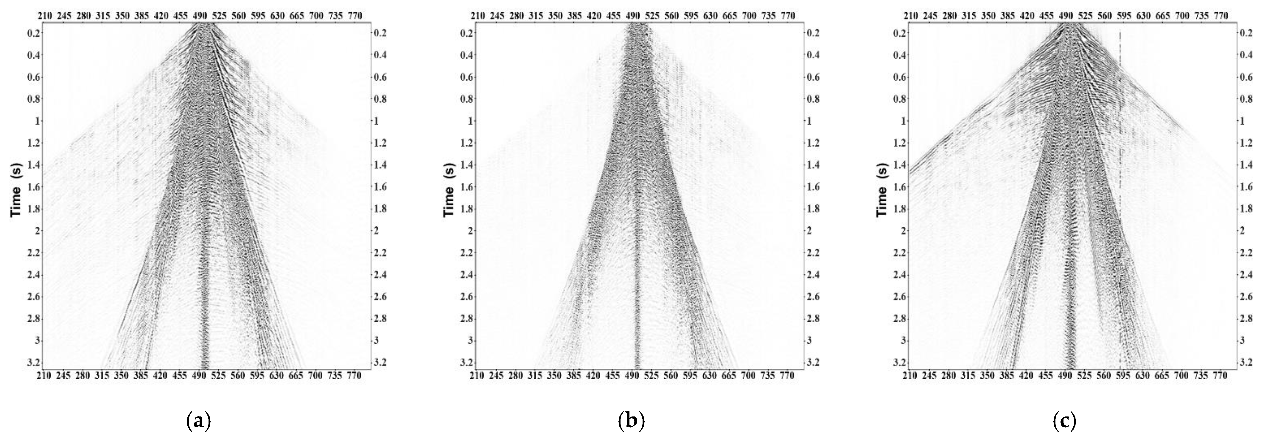
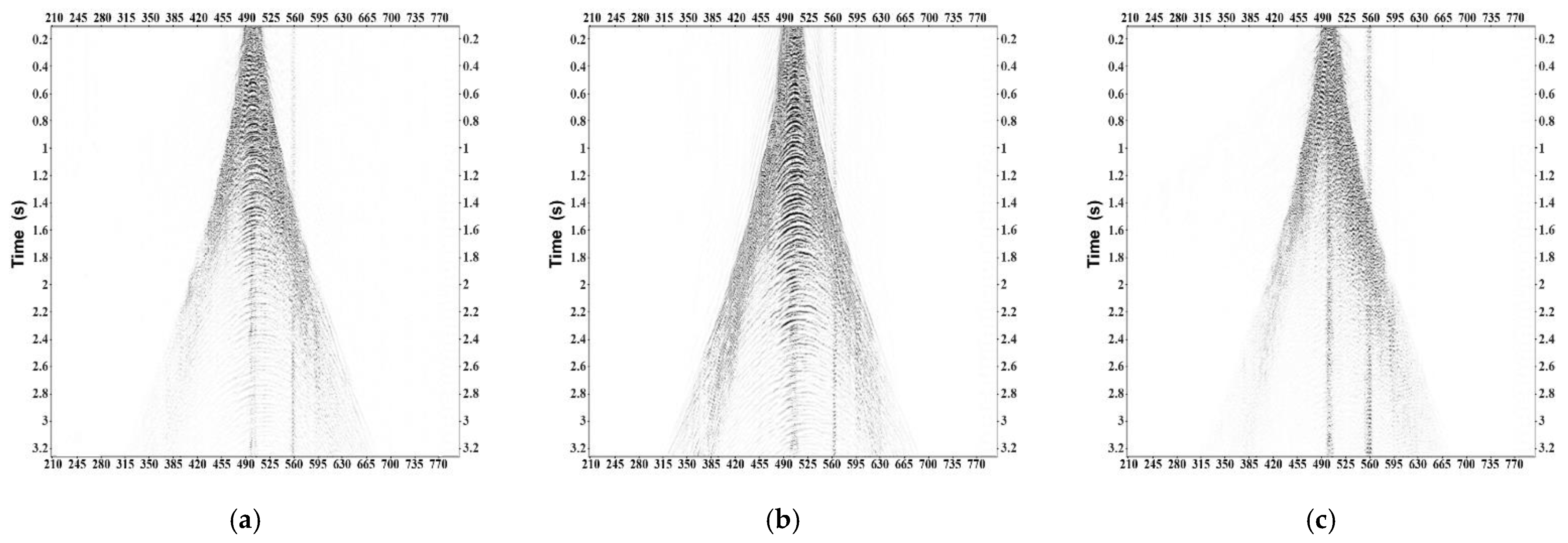
Figure 4 shows a single-shot record of the P-wave source in the study area; theoretically, the seismic records generated by P wave sources do not have shear wave fields. As shown in Figure 4a, with the X-component wave field seismic record of the P-wave source, the wave field is relatively complex, the converted wave signal is relatively weak and submerged in a large amount of scattering noise, and there is obvious leaked pure shear wave information in the near trace. The Y-component wave field seismic record is shown in Figure 4b; there is basically no converted wave information in this component, and the near trace is dominated by noise with weak pure shear wave information. The Z-component wave field seismic record is shown in Figure 4c; the P-wave reflection hyperbola characteristics of the shallow part are relatively obvious in this wave field, the near-trace is dominated by noise without pure shear wave information, and the deep information is submerged in a large amount of scattered noise. The reason why the converted wave signal of the P-wave field is relatively weak and the effective information of the wave field is submerged in a large amount of scattered noise is likely due to the fact that the area is a biogas enrichment area in relatively deep strata based on the geological characteristics of the area, which is also the reason why the use of P-wave data for reverse time migration imaging in this area is not ideal.
Figure 5 shows the corresponding single-shot record obtained from the SH shear wave source (i.e., the y-direction concentrated force source) in this area. As shown in Figure 5a, the X-component data, there should be no SH shear wave information in isotropic media, but there is relatively weak SH shear wave signal leakage in actual data. The most likely cause of SH shear wave signal leakage is due to shear-wave splitting, which is not the focus of this article. The seismic record of the Z-component wave field in Figure 5c is dominated by noise without SH shear wave information, which is consistent with the theory of the SH shear wave propagation. In theory, the wave field obtained by concentrating force sources in the y-direction only has wave field information in the Y-component in isotropic media. Figure 5b is the seismic record of the y-component wave field, with a high signal-to-noise ratio and obvious SH shear wave information. Overall, the resolution of SH shear wave seismic records is higher than that of P-wave seismic record, comparing Figure 5b with Figure 4c. SH shear wave source data can also have a high signal-to-noise ratio in the deep gas cloud region due to its insensitivity to gas, and it has great advantages in geological structure characterization and reverse time migration imaging research in this area.
It can be seen through the analysis of shot records that the data quality of the SH-Y component is relatively good. This research focuses on imaging research on SH-Y component data. This component is perpendicular to the survey line direction.
4.2. Depth Domain Imaging Matching and Velocity Model Building
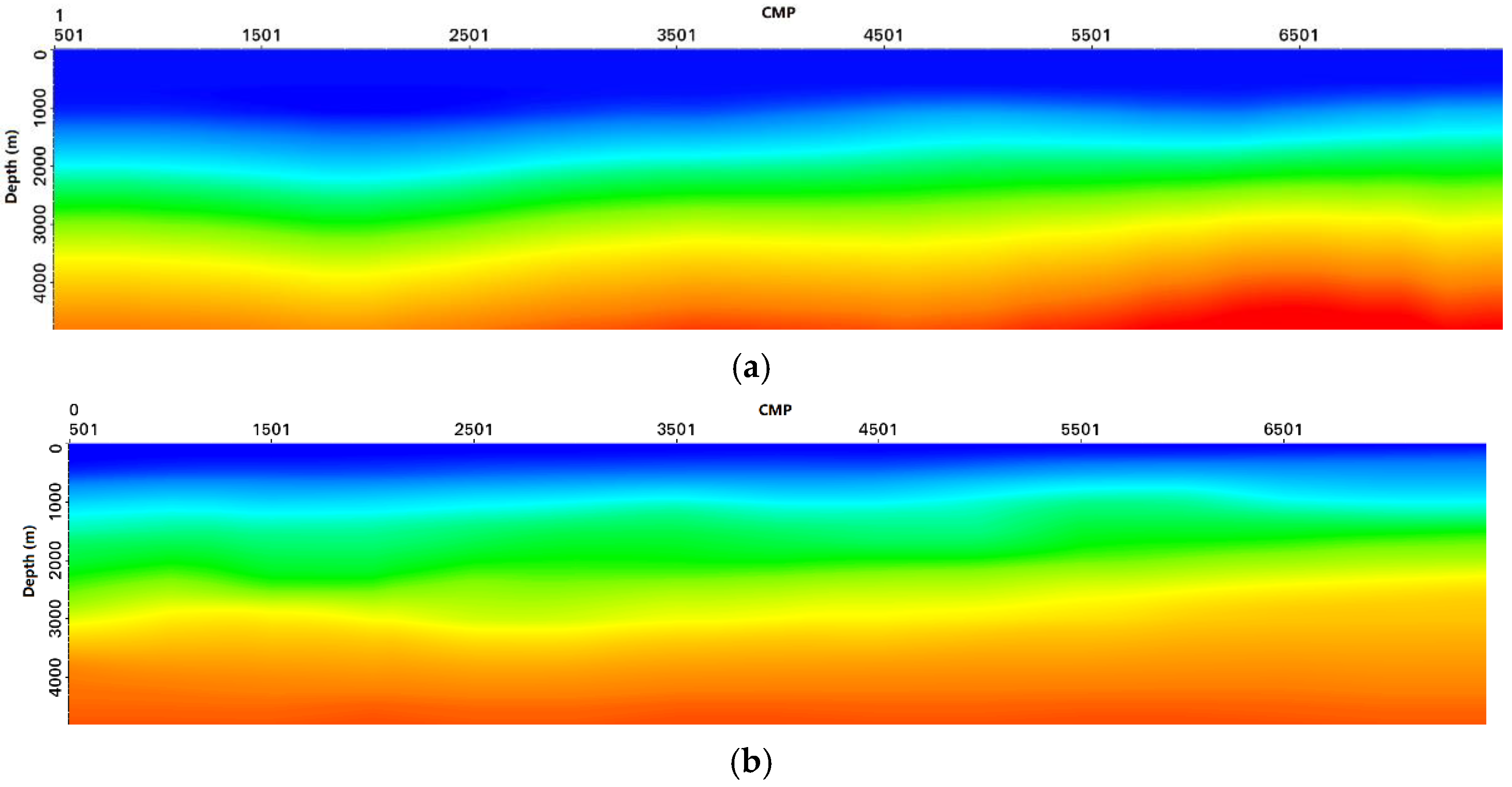
The depth domain velocity model of the P-wave and SH shear wave have been established, respectively, with a velocity model building workflow including layer- and grid-based tomography. It is shown in Figure 6 with the depth domain velocity models of the P-wave and SH shear wave, respectively, that they have a certain similarity in the spatial variation of the velocity field; the velocity of the P-wave is relatively low at the position of CMP (common middle point) 1200–2500, and it is relevant to the gas enrichment in this area, which can also be seen in the pre-stack depth migration results shown later.
The imaging of the reflector of the P-wave and the strong reflector of the SH shear wave should be located at the same depth because the pre-stack depth migration images show the wave impedance interface of subsurface media. It is very difficult to match the depth domain imaging positions of the P-wave and SH shear wave in practical applications due to the low signal-to-noise ratio of P-wave data, the possibility of anisotropy, and various uncertainties in the area. A relatively easy-to-implement process has been designed to attempt to match the imaging depth of the P-wave and SH shear wave. Our idea is to constrain VP and vs. because the most significant factor affecting the imaging depth is the velocity field. The specific method is that a set of strong reflectors in the survey are selected; they are picked up in the migration images of the P-wave and SH shear wave, respectively; and their average velocities are calculated from the surface to the reflectors. The specific formula is , in which, for , , similar calculations for both the P-wave and SH shear wave have been made, the imaging position of the strong reflector in the depth domain is determined by this average velocity, and the average velocity ratio obtained should also be consistent with the P-wave and SH shear wave velocity in the survey [40]. The existing depth domain velocity can be corrected if the velocity ratio of SH shear wave and SH shear wave in the space of the survey is obtained. The pre-stack time migration images have been used and the corresponding reflectors have been picked up to solve this problem, the pre-stack time images of the P-wave and SH shear wave approximately represent the vertical two-way travel time of the P-wave and SH shear wave with zero offset, and the travel time ratio is obtained to further constrain the VS/VP ratio.
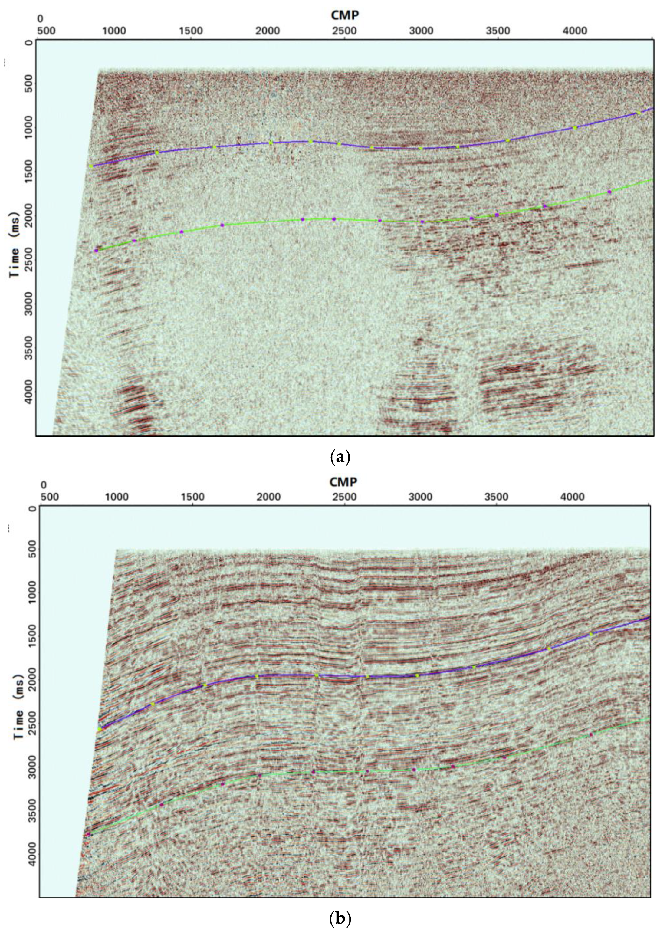
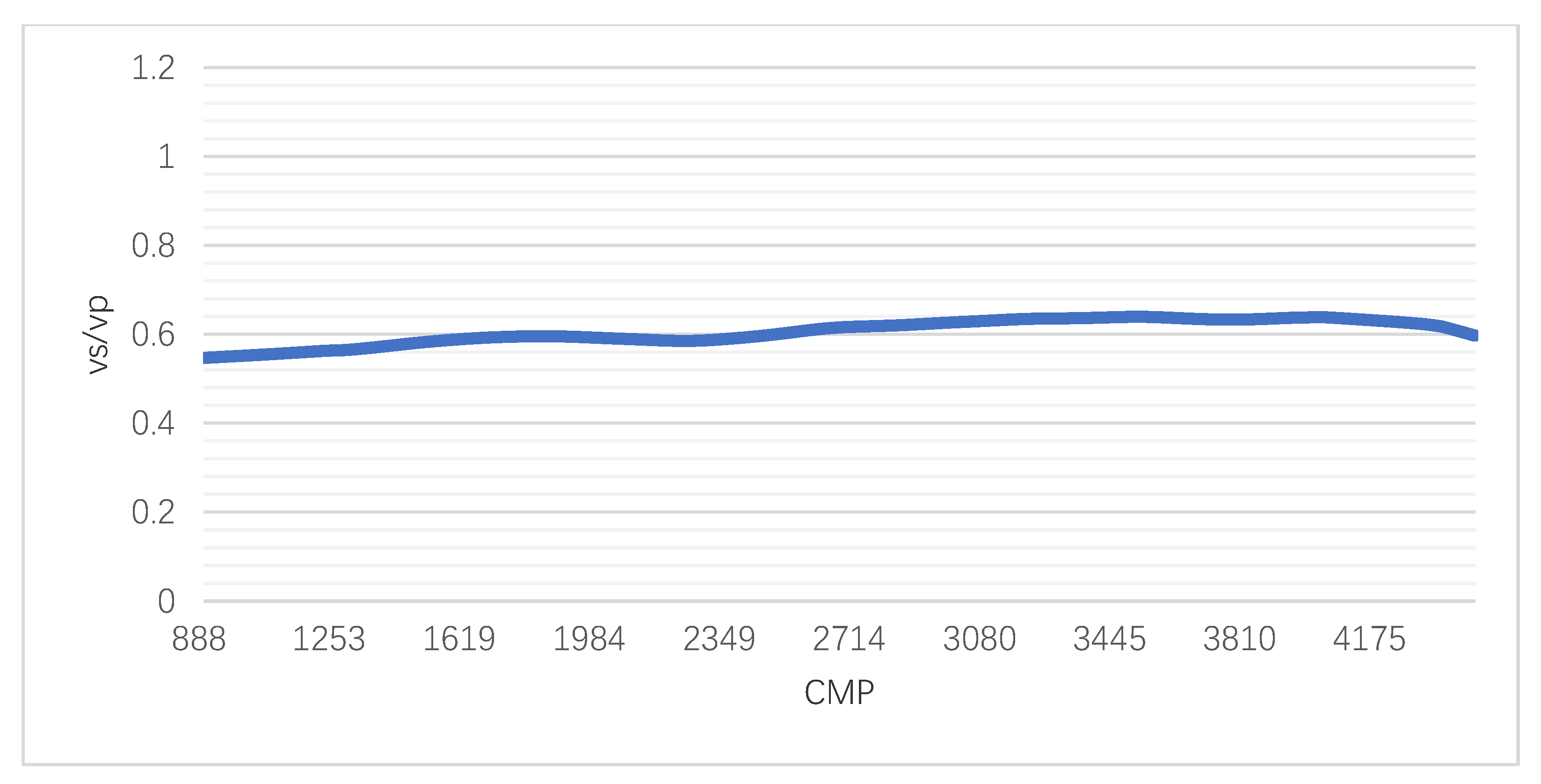
Back to the first step, a corresponding proportional constraint has been made on the P-wave velocity field with a correction of about 1–3%, and the weak anisotropy parameter is utilized to solve the residual moveout of imaging caused by this correction. In fact, the numerical model verifies that isotropic and anisotropic imaging profiles are close to each other under weak anisotropy (<5%); therefore, anisotropy is ignored in this study [41]. In Figure 7, the horizon selected for the P-wave and SH shear wave in the time domain is used to calculate the P-wave and SH shear wave velocity ratio. Figure 8 shows the P-wave and SH shear wave velocity ratio.
For ease of understanding, we built a flow chart of velocity modeling, as shown in Figure 9. Figure 9 is about the P wave and SH shear wave velocity modeling process in this paper. In this figure, for the convenience of display, the S wave means SH shear wave. We can see that, after the preliminary modeling, we need to go through layer-based tomography and grid-based tomography, and the velocity ratio is obtained simultaneously with the velocity modeling. After the velocity ratio is obtained, it is used to constrain the velocity model of P wave to get the accurate velocity model.
4.3. RTM Results of P and SH Shear Wave
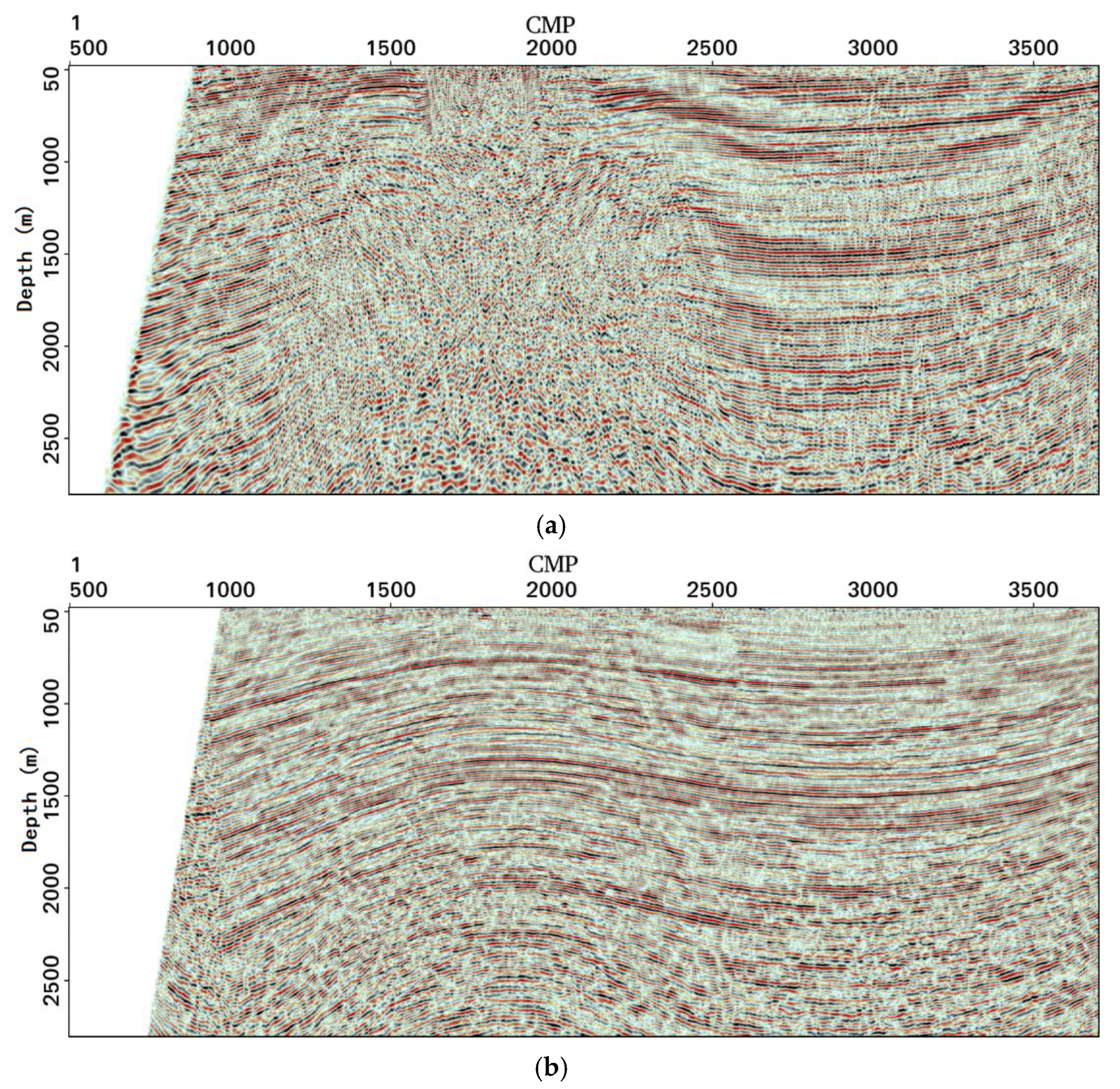
The reverse time migration of P-wave and SH shear wave data were carried out, respectively; there are 1519 shots and 8472 detection points in this survey, and the same acquisition geometry was adopted for both the P- and SH shear wave. The eighth-order finite difference scheme with a variable grid was adopted for P-wave reverse time migration for seismic wave simulation, the imaging condition is the cross-correlation imaging condition, and we use Laplace filtering to remove the low-frequency noise of the imaging. The SH shear wave reverse time migration was realized on a regular grid with the sixth-order CCD (Formula (3)) wave field simulation method adopted, an interval of 2 m for the grid size in the z-direction and an interval of 5 m for the grid size in the x-direction were adopted, and Laplace filtering was adopted to remove the low-frequency noise of the imaging to ensure stability and suppress alias frequencies in the wave field continuation process. Figure 10 shows the pre-stack depth migration images of the P-wave and SH shear wave. It can be seen in the image that there is no clear reflector for the P-wave in the area of CMP (common middle point) 1200–2500, which is due to the gas cloud in the area; the P-wave is significantly absorbed and has difficulty in passing through the area and reflecting to the surface when the compression wave goes through the area, but the SH shear wave can propagate normally in the area because it propagates through the rock frame and is not affected by the gas. Therefore, SH shear wave reverse time migration can clearly image through this area and has obvious imaging advantages in this area over P-wave.
5. Conclusions
The depth domain pre-stack migration practice was performed for P-wave and SH shear wave seismic data in the Sanhu area of the Qaidam Basin in Qinghai Province, including depth domain velocity model building, P-wave to SH shear wave velocity ratio estimation, and reverse time migration (RTM). The layer- and grid-based tomography methods were used to build the depth velocity model. Additionally, the pre-stack time migration results of the P-wave and SH shear wave were utilized to approximately calculate the distribution of the P-wave and SH shear wave velocity ratio in the study area, and the ratio was used to constrain the P-wave and SH shear wave velocity model building so that the reflectors of the P-wave and SH shear wave pre-stack depth migration results were matched in the depth domain. An eighth-order finite difference scheme was used for P-wave RTM on a variable grid, and a sixth-order CCD was used for SH shear wave RTM on a regular grid. The results showed that the SH shear wave results have obvious imaging advantages compared with the P-wave results in the gas-cloud region, which verified the accuracy of the SH shear wave RTM algorithm and demonstrated great potential in seismic imaging application.
Author Contributions
Conceptualization, C.Z.; Formal analysis, J.Y.; Funding acquisition, X.L.; Investigation, C.Z., W.Y. and H.N.; Methodology, C.Z. and W.Y.; Project administration, J.Y. and X.L.; Resources, J.Y. and H.N.; Software, C.Z.; Supervision, X.L.; Validation, H.N.; Writing—original draft, C.Z. and W.Y.; Writing—review & editing, X.L. All authors have read and agreed to the published version of the manuscript.
Funding
The study is supported by the Science and Technology Research and Development Project of CNPC (2021DJ3506) and (2021ZG03) and R&D Department of China National Petroleum Corporation (Investigations on fundamental experiments and advanced theoretical methods in geophysical prospecting applications, 2022DQ0604-02).
Institutional Review Board Statement
Not applicable.
Informed Consent Statement
Not applicable.
Data Availability Statement
Not applicable.
Conflicts of Interest
The authors declare no conflict of interest.
References
- Gou, L.; Zhang, S.; Li, X. Improving the Effectiveness of Shear-wave Seismic Exploration through Geophysical Technology Innovation. Pet. Sci. Technol. Forum 2021, 40, 12–19. [Google Scholar]
- Shao, Z.; He, S.; Hou, L.; Wang, Y.; Tian, C.; Liu, X.; Zhou, Y.; Hao, M.; Lin, C. Dynamic Accumulation of the Quaternary Shale Biogas in Sanhu Area of the Qaidam Basin, China. Energies 2022, 15, 4593. [Google Scholar] [CrossRef]
- Bouchaala, F.; Guennou, C. Estimation of viscoelastic attenuation of real seismic data by use of ray tracing software: Application to the detection of gas hydrates and free gas. Comptes Rendus Geosci. 2012, 344, 57–66. [Google Scholar] [CrossRef]
- Matsushima, J.; Ali, M.Y.; Bouchaala, F. A novel method for separating intrinsic and scattering attenuation for zero-offset vertical seismic profiling data. Geophys. J. Int. 2017, 211, 1655–1668. [Google Scholar] [CrossRef]
- Li, X.; Zhang, S. Forty years of shear-wave splitting in seismic exploration: An overview. Geophys. Prospect. Pet. 2021, 60, 190–209. [Google Scholar]
- Gaiser, J.E. 3-D converted shear wave rotation with layer stripping. U.S. Patent US5610875, 11 March 1997. [Google Scholar]
- Wu, Y.; He, Z.; He, J.; Deng, Z.; Wang, Y.; Yin, W. P-wave and S-wave joint acquisition technology and its application in Sanhu Area. In SEG Technical Program Expanded Abstracts 2018; Society of Exploration Geophysicists: Tulsa, OK, USA, 2018; pp. 1–5. [Google Scholar]
- Takougang, E.M.T.; Ali, M.Y.; Bouzidi, Y.; Bouchaala, F.; Sultan, A.A.; Mohamed, A.I. Characterization of a carbonate reservoir using elastic full-waveform inversion of vertical seismic profile data. Geophys. Prospect. 2020, 68, 1944–1957. [Google Scholar] [CrossRef]
- Dai, F.; Zhang, F.; Li, X.-Y. SH-SH wave inversion for S-wave velocity and density. Geophysics 2022, 87, A25–A32. [Google Scholar] [CrossRef]
- Zhang, F. Simultaneous inversion for S-wave velocity and density from the SV-SV wave. Geophysics 2021, 86, R187–R195. [Google Scholar] [CrossRef]
- LI, X.Y. Processing P-P and P-S waves in multicomponent sea-floor data for azimuthal anisotropy: Theoryandoverview. Oil Gas Sci. Technol. 1998, 53, 607–620. [Google Scholar]
- Zhang, F.; Li, X. Inversion of the reflected SV-wave for density and S-wave velocity structures. Geophys. J. Int. 2020, 221, 1635–1639. [Google Scholar] [CrossRef]
- Cheng, J.W.; Zhang, F.; Li, X.Y. Nonlinear amplitude inversion using a hybrid quantum genetic algorithm and the exact zoeppritz equation. Pet. Sci. 2022, v, 1048–1064. [Google Scholar] [CrossRef]
- Cheng, J.W.; Zhang, F.; Li, X.Y. Seismic Amplitude Inversion for Orthorhombic Media Based on a Modified Reflection Coefficient Approximation. Surv. Geophys. 2022, v, 1–39. [Google Scholar] [CrossRef]
- Deng, Z.; Li, C.; Chen, G.; Yang, J.; Wang, R.; Hu, Y.; An, S.; Wang, H.; Du, Z. The application of pure shear wave seismic data for gas reservoir delineation. In SEG Technical Program Expanded Abstracts 2019; Society of Exploration Geophysicists: Tulsa, OK, USA, 2019; pp. 2690–2694. [Google Scholar]
- Brian, R.; Larry, L. A Gassmann consistent rock physics template. CSEG Rec. 2013, 38, 22–30. [Google Scholar]
- Li, X.Y. Fractured reservoir delineation using multicomponent seismic data. Geophys. Prospect. 1997, 45, 39–64. [Google Scholar] [CrossRef]
- Chang, W.; McMechan, G.A. 3-D elastic prestack, reverse-time depth migration. Geophysics 1994, 59, 597–609. [Google Scholar] [CrossRef]
- Du, Q.Z.; Zhu, Y.T.; Ba, J. Polarity reversal correction for elastic reverse time migration. Geophysics 2012, 77, S31–S41. [Google Scholar] [CrossRef]
- Dai, N.; Wu, W.; Zhang, W.; Wu, X. TTI RTM using variable grid in depth. Int. Pet. Technol. Conf. 2011, v, 1–7. [Google Scholar]
- Zhang, J.; Tian, Z.; Wang, C. P- and S-wave separated elastic wave equation numerical modeling using 2D staggered-grid. In Proceedings of the 77th Annual International Meeting, SEG, San Antonio, TX, USA, 14 September 2007; pp. 2104–2109. [Google Scholar]
- Xiao, X.; Leaney, W.S. Local vertical seismic profiling (VSP) elastic reverse-time migration and migration resolution: Salt-flank imaging with transmitted P-to-S waves. Geophysics 2010, 75, S35–S49. [Google Scholar] [CrossRef]
- Gu, B.; Li, Z.; Ma, X.; Liang, G. Multi-component elastic reverse time migration based on the P and S separating elastic velocity-stress equation. J. Appl. Geophys. 2015, 112C, 62–78. [Google Scholar] [CrossRef]
- Wang, W.; McMechan, G.A.; Zhang, Q. Comparison of two algorithms for isotropic elastic P and S decomposition in the vector domain. Geophysics 2015, 80, T147–T160. [Google Scholar] [CrossRef] [Green Version]
- Du, Q.; Gong, X.; Zhang, M.; Zhu, Y.; Fang, G. 3D PS-wave imaging with elastic reverse-time migration. Geophysics 2014, 79, S173–S184. [Google Scholar] [CrossRef]
- Zhang, Q.; McMechan, G.A. 2D and 3D elastic wavefield vector decomposition in the wavenumber domain for VTI media. Geophysics 2010, 75, D13–D26. [Google Scholar] [CrossRef]
- Du, Q.Z.; Guo, C.F.; Zhao, Q.; Gong, X.; Wang, C.; Li, X.Y. Vector-based elastic reverse time migration based on scalar imaging condition. Geophysics 2017, 82, S111–S127. [Google Scholar] [CrossRef]
- Nguyen, B.D.; McMechan, G.A. Five ways to avoid storing source wavefield snapshots in 2D elastic prestack reverse time migration. Geophysics 2015, 80, S1–S18. [Google Scholar] [CrossRef]
- Tian, J.; Zeng, X.; Wang, W.; Shaosheng, Z.; Zeqing, G.; Hua, K. The detection of biogas in unconsolidated sandstone formation of the Qua-ternary in Qaidam Basin. Geophys. Prospect. Pet. 2016, 55, 408–413. [Google Scholar]
- Sun, P.; Guo, Z.-Q.; Zhang, L.; Tian, J.-X.; Zhang, S.-S.; Zeng, X.; Kong, H.; Yang, J. Biologic gas accumulation mechanism and exploration strategy in Sanhu area, Qaidam Basin. Nat. Gas Geosci. 2013, 24, 494–504. [Google Scholar]
- Chen, G.; Deng, Z.; Jiang, T.; Junyong, Z.; Xuejiao, Y.; Chengye, Q.; Xiaoping, X. Application of PP-wave and SS-wave joint interpretation technology in gas cloud area. Lithol. Reserv. 2019, 31, 79–87. [Google Scholar]
- Zhu, T.; Harris, J.M.; Biondi, B. Q-compensated reverse-time migration. Geophysics 2014, 79, S77–S87. [Google Scholar] [CrossRef]
- Helene, H.V.; Martin, L. Simultaneous inversion of PP and PS seismic data. Geophysics 2006, 71, R1–R10. [Google Scholar]
- Ruixue, S.; Ayse, K.; Christopher, J. High resolution seismic reflection PP and PS imaging of the bedrock surface below glacial deposits in Marsta, Sweden. J. Appl. Geophys. 2022, 198, 1–13. [Google Scholar]
- Chu, P.C.; Fan, C.W. A three-point combined compact difference scheme. J. Comput. Phys. 1998, 140, 370–399. [Google Scholar] [CrossRef] [Green Version]
- Dong, L.; Zhan, J. Combined super compact finite difference scheme and application to simulation of shallow water equations. Chin. J. Comput. Mech. 2008, 25, 791–796. [Google Scholar]
- Sengupta, T.K.; Ganeriwal, G.; De, S. Analysis of central and upwind compact schemes. J. Comput. Phys. 2003, 192, 677–694. [Google Scholar] [CrossRef]
- Wu, G.C.; Wang, H.Z. Analysis of numerical dispersion in wave 2 field simulation. Prog. Geophys. 2005, 20, 58–65. [Google Scholar]
- Zhou, C.; Wu, W.; Sun, P.; Yin, W.; Li, X. The Combined Compact Difference Scheme Applied to Shear-Wave Reverse-Time Migration. Appl. Sci. 2022, 12, 7047. [Google Scholar] [CrossRef]
- Brian, R.; Hedlinz, K.; Hilterman, F.J.; Lines, R. Tutorial Fluid-property discrimination with AVO: A Biot-Gassmann perspective. Geophysics 2003, 68, 29–39. [Google Scholar]
- Jin, S. Tying PS to PP depth section: Two examples of anisotropic prestack depth imaging of 4C data. In SEG Technical Program Expanded Abstracts 2002; Society of Exploration Geophysicists: Tulsa, OK, USA, 2002. [Google Scholar]
Figure 1.
Pre-stack time migrated P-wave seismic section in a gas-cloud region of Sanhu.

Figure 2.
Velocity ratio curves for different numerical simulation methods. The blue curve is the traditional central difference scheme, the green curve is the traditional implicit difference scheme, the red curve is the CCD difference scheme and the black line is the velocity ratio constant of 1: (a) ; (b) ; (c) .

Figure 3.
Relative errors of numerical simulation for different schemes and gird size: (a) Δx = 10 m, Δt = 0.001 s; (b) Δx = 15 m, Δt = 0.001 s.
Figure 3.
Relative errors of numerical simulation for different schemes and gird size: (a) Δx = 10 m, Δt = 0.001 s; (b) Δx = 15 m, Δt = 0.001 s.

Figure 4.
(a) The X-component wave field seismic record of the P-wave source. (b) The Y-component wave field seismic record of the P-wave source. (c) The Z-component wave field seismic record of the P-wave source.
Figure 4.
(a) The X-component wave field seismic record of the P-wave source. (b) The Y-component wave field seismic record of the P-wave source. (c) The Z-component wave field seismic record of the P-wave source.

Figure 5.
(a) The X-component wave field seismic record of the SH shear wave source. (b) The Y-component wave field seismic record of the SH shear wave source. (c) The Z-component wave field seismic record of the SH shear wave source.
Figure 5.
(a) The X-component wave field seismic record of the SH shear wave source. (b) The Y-component wave field seismic record of the SH shear wave source. (c) The Z-component wave field seismic record of the SH shear wave source.

Figure 6.
(a) The depth domain velocity model of the P-wave with a velocity model building workflow including layer- and grid-based tomography. (b) The corresponding depth domain velocity model of the SH shear wave.
Figure 6.
(a) The depth domain velocity model of the P-wave with a velocity model building workflow including layer- and grid-based tomography. (b) The corresponding depth domain velocity model of the SH shear wave.

Figure 7.
Pre-stack time migration (PSTM) sections: (a) P-wave and (b) SH shear wave.

Figure 8.
VS/VP ratio in the survey.

Figure 9.
Velocity modeling flowchart.

Figure 10.
Pre-stack depth migration sections using RTM: (a) the P-wave, Δx = 5 m, Δz = 2 m; (b) the SH shear wave, Δx = 5 m, Δz = 2 m.
Figure 10.
Pre-stack depth migration sections using RTM: (a) the P-wave, Δx = 5 m, Δz = 2 m; (b) the SH shear wave, Δx = 5 m, Δz = 2 m.

Publisher’s Note: MDPI stays neutral with regard to jurisdictional claims in published maps and institutional affiliations. |
© 2022 by the authors. Licensee MDPI, Basel, Switzerland. This article is an open access article distributed under the terms and conditions of the Creative Commons Attribution (CC BY) license (https://creativecommons.org/licenses/by/4.0/).
Share and Cite
MDPI and ACS Style
Zhou, C.; Yin, W.; Yang, J.; Nie, H.; Li, X. Reverse Time Migration Imaging Using SH Shear Wave Data. Appl. Sci. 2022, 12, 9944. https://0-doi-org.brum.beds.ac.uk/10.3390/app12199944
AMA Style
Zhou C, Yin W, Yang J, Nie H, Li X. Reverse Time Migration Imaging Using SH Shear Wave Data. Applied Sciences. 2022; 12(19):9944. https://0-doi-org.brum.beds.ac.uk/10.3390/app12199944
Chicago/Turabian StyleZhou, Chengyao, Wenjie Yin, Jun Yang, Hongmei Nie, and Xiangyang Li. 2022. "Reverse Time Migration Imaging Using SH Shear Wave Data" Applied Sciences 12, no. 19: 9944. https://0-doi-org.brum.beds.ac.uk/10.3390/app12199944
Note that from the first issue of 2016, this journal uses article numbers instead of page numbers. See further details here.