Article

Machine Learning Techniques Applied to Identify the Two-Phase Flow Pattern in Porous Media Based on Signal Analysis

State Key Laboratory of Multiphase Flow in Power Engineering, Xi’an Jiaotong University, Xian-Ning West Road 28#, Xi’an 710049, China
*
Author to whom correspondence should be addressed.
Submission received: 29 July 2022 / Revised: 18 August 2022 / Accepted: 24 August 2022 / Published: 27 August 2022
(This article belongs to the Special Issue Flow and Heat Transfer Research in Multiphase Flow and Porous Media)

Abstract

:
The development of flow pattern identification technology for gas–liquid two-phase flow in porous media is of great significance to engineering research and production. In this paper, a high accuracy identification method for two-phase flow pattern in porous media is proposed with Machine learning techniques. The gas–liquid two-phase flow patterns and corresponding differential pressure signals in porous beds with particle diameters of 1.5 mm, 3 mm, and 6 mm are obtained through visual experiments. Three time domain characteristic parameters (Mean, Standard deviation, and Range) are calculated by a statistical method, while the EMD energy spectrum of the signal is obtained by empirical mode decomposition. Based on these parameters, machine learning technology, including support vector machine (SVM) and BP neural network, are employed to identify the flow pattern. Four flow pattern identification models are trained based on SVM and BP neural network, with accuracies of 94.77%, 93.4%, 96.08%, and 91.5%. Furthermore, the three models with good performance are integrated by integrated learning technology. An integrated identification model of gas–liquid two-phase flow pattern in porous media with an overall accuracy of 98.04% is finally obtained.

1. Introduction

Two-phase flow in porous media plays a critical role in scientific and industrial processes. During a severe accident of a light water reactor (LWR), the corium may form a debris bed with a porous media structure [1]. Understanding the two-phase flow mechanism in porous media is important to developing efficient cooling technology and terminating severe accidents. In petroleum engineering applications, since the oil–water mixtures are stored in the underground cracks of porous media structures, the study of two-phase flow in porous media is conducive to the development of more efficient oil extraction technologies [2]. In addition, in agriculture engineering [3], chemical engineering [4], and other fields, two-phase flow in porous media also widely exists and has an important impact on experiments and production. Flow pattern, which has a great effect on heat and mass transfer, is the research foundation to clarify the flow and heat transfer mechanism of two-phase flow in porous media as well as improve industrial production efficiency [5]. Accurate identification of flow patterns is the premise of flow pattern research. For the needs of experiments and industrial production, it is of great significance to develop accurate and fast flow pattern identification technology for porous media.
In early research, scholars directly observe the two-phase flow patterns in transparent pipes (including pipes filled with porous media) with their eyes. They distinguish different flow patterns according to the forms of the gas–liquid phase [6,7]. Afterward, the application of high-speed cameras helps the researchers capture the subtle changes in flow patterns timely and accurately [8]. This direct observation method is very effective for classifying and identifying typical flow patterns. However, it also has some limitations. For example, in real production, there are few transparent pipelines, which limits direct observation. In addition, for the transition flow pattern between typical flow patterns, it is difficult to distinguish which flow pattern it belongs to only through observation since it will be disturbed by the subjectivity of the observer.
In order to solve the above problems, scholars try to improve the flow pattern identification method. Some scholars try to establish experimental systems in the laboratory to simulate the real situation. Using these devices, scholars have observed various flow patterns and obtained some corresponding signals that are easy to be measured, such as differential pressure signals [9,10,11], temperature signals [12], and so on. After extracting the features of these signals and classifying them according to the corresponding flow patterns, the relationship between different flow patterns and signal features can be established, which is the basis for flow pattern judgment. The signal feature extraction techniques can be divided into three categories: time domain feature extraction, frequency domain feature extraction, and time-frequency domain feature extraction. Time domain feature extraction includes mean value, variance, and probability density function (PDF), etc. The common method of frequency domain feature extraction is power spectral density (PSD). Time-frequency analysis technology appears late, including wavelet analysis, empirical mode decomposition (EMD), and Hilbert-Huang transform [13]. Matsui [14] calculated the probability density function (PDF) of the differential pressure signal and distinguished the flow pattern by the shape of the PDF curve. Elperin and Klochko [15] extracted the wavelet energy spectrums of differential pressure signals to distinguish the flow patterns. dos Reis [16] summarized the characteristics of power spectral density (PSD) and PDF of the capacitive probe signal of slug flow. Li [17] identified the flow pattern in the dust collector through the synthesis of PSD, PDF, and wavelet features. Wu [10] characterized different flow regimes and their transition in a concentric vertical annulus through autocorrelation, PSD, Shannon entropy, and permutation entropy.
In recent years, machine learning technology has been developed in industries greatly [18,19,20,21]. It shows a strong ability in pattern recognition and classification, which provides a reference for the progress of flow pattern identification technology. More and more scholars have applied machine learning technology to the field of flow pattern recognition and developed a series of well-performing flow pattern recognition methods. Liang [22] used ultrasonic echoes and RBF neural network to identify the flow patterns in a horizontal pipe. Pei [23] utilized the complex network theory to identify the flow patterns in water pipelines. Guo [12] applied a neural network with the temperature fluctuation on pipe walls in classifying flow patterns. In addition to neural networks, support vector machine (SVM) technology is also widely used in flow pattern recognition. Zhang [24] identified the oil–gas two-phase flow pattern based on SVM and electrical capacitance tomography technique. Liu [25] used doppler spectrum analysis and SVM to identify the flow pattern of oil–water two-phase flow. Ambrosio [26] used void fraction time series and SVM to classify the two-phase flow pattern in a vertical pipe.
It can be seen that the flow pattern recognition method combining signal feature extraction and machine learning technology has been introduced on some occasions. Unfortunately, compared with the importance of two-phase flow pattern identification in porous media, the research on this technology is far from enough. The present study proposes a new method to identify the gas–liquid two-phase flow pattern in porous media based on differential pressure signals and machine learning technology. The time domain characteristics and time-frequency domain (EMD) characteristics of the differential pressure signal are obtained. Using these features, a variety of flow pattern identification models based on SVM and BP neural networks are constructed. The comparison of different models verifies the performance of SVM and BP neural networks in porous media flow pattern recognition. Finally, an intelligent online flow pattern identification system for porous media is constructed by using three optimal models and integrated recognition technology. Compared with the single model, the identification ability of the system has been improved. This paper provides a new idea for the development of flow pattern identification methods in porous media in the fields of the chemical industry, agriculture, petroleum, and nuclear engineering.

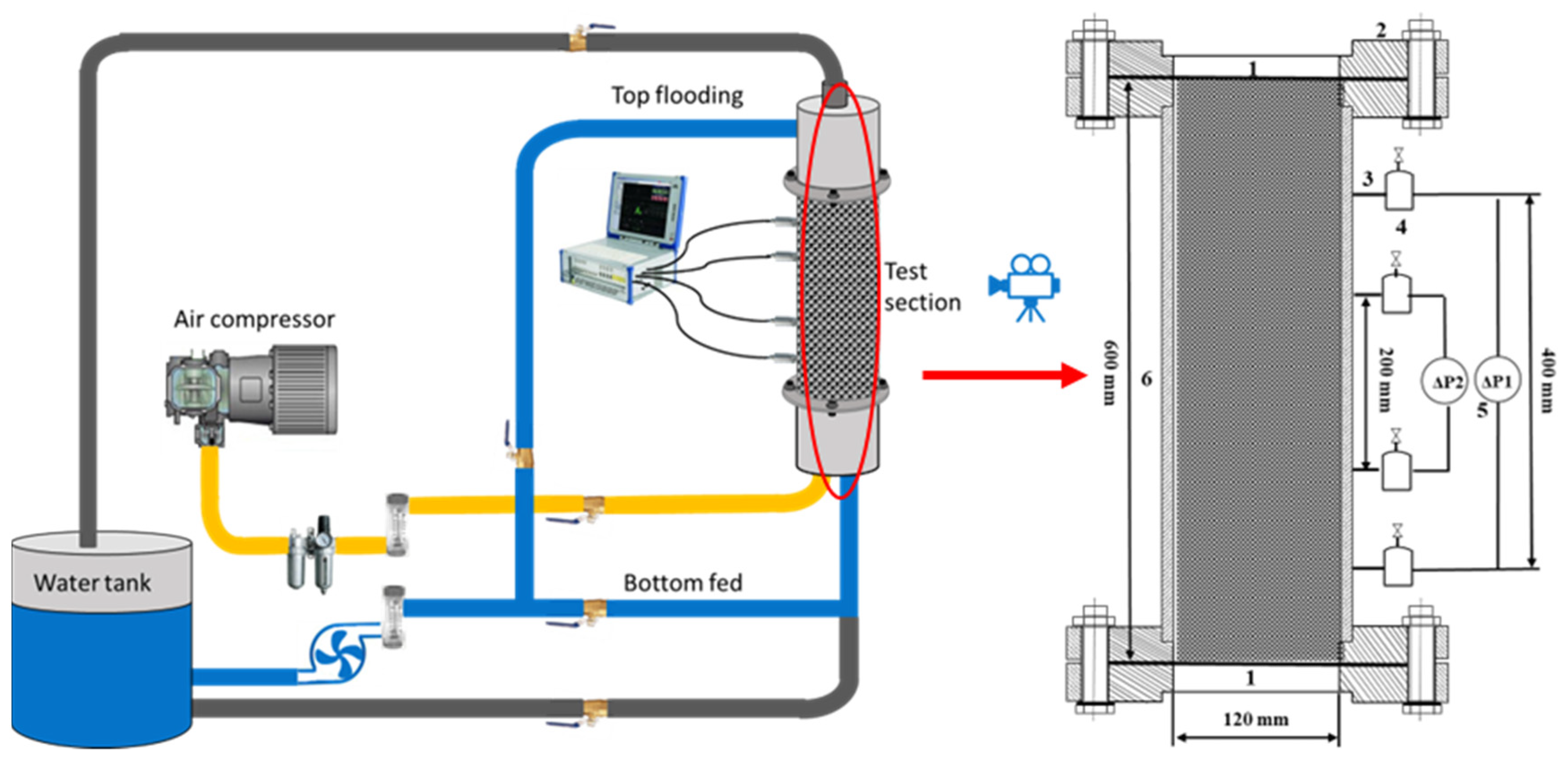
2. Description of Experiments

The experiments are carried out on a visual experimental system named DEBECO-LT (Debris Bed Coolability-Low Temperature). Figure 1 shows the diagram of the experimental system. In this paper, air and water are sent to the bottom of the test section, where they mix and flow into the porous media pipe. The wall of the experimental section is made of plexiglass, and two stainless steel wire meshes are fixed at the top and bottom to ensure that the glass balls will not move casually. Rosemont-3051 transmitters (0.04%) are fixed at the inlet and outlet of the test section to measure the differential pressure signals; the signal acquisition frequency is 400 Hz. FastcamMini Photron high-speed camera (102, 400 frame/s) is used to capture clear flow pattern photos. The previous paper describes the experimental system in more detail [27].
The experimental pressure is equal to the local atmospheric pressure, about 0.1 MPa. The room temperature is about 10 °C. Spherical glass particles with diameters of 1.5 mm, 3 mm, and 6 mm are packed into three different porous media beds. The superficial velocity of air is 0.005–0.44 m/s and that of water is 0.59–1.17 mm/s. More details of the experimental setup can be found in Table 1.

3. Methodology

3.1. Feature Extraction Methodology

Feature extraction is the key to establishing the relationship between flow patterns and signals, and it is also the basis of machine learning technology to distinguish and recognize flow patterns. Appropriate feature extraction is important to developing flow pattern identification technology. In this paper, statistical methods and empirical modal analysis (EMD) technology are used to extract the time domain and time-frequency domain characteristics of the signal.

3.1.1. Characteristics of Time Domain

In this paper, three common statistical parameters, which are mean, variance, and range of the signal, are selected to reflect the time domain characteristics of the signal. These features can be used to analyze the time domain features of signals and as the input of machine learning classifiers containing time domain features. The calculation formulas are as follows:
Mean of differential pressure signal:
m = 1 N i = 1 N s ( i )
where x(i) refers to each point of the signal, and N indicates the number of signal points.
The standard deviation of differential pressure signal:
S = 1 N i = 1 N ( s ( i ) m ) 2
where m refers to the mean of the differential pressure signal
Range of differential pressure signal:
R = s ( i ) max s ( i ) min

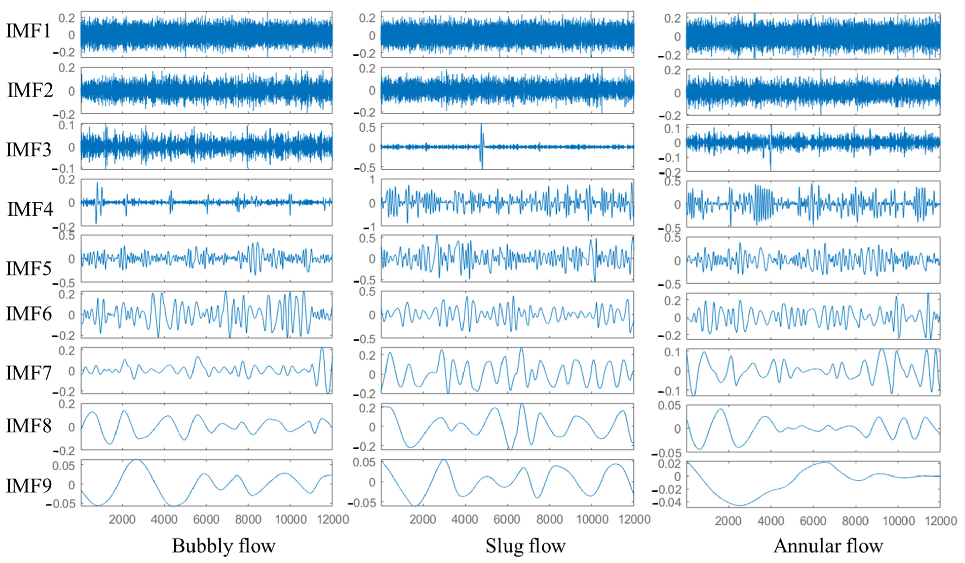
3.1.2. Characteristics of Time-Frequency Domain

It is not comprehensive to extract the signal features only from the time domain. In order to extract more abundant features, this paper also introduces the empirical mode decomposition (EMD) method to extract the time-frequency domain features of the signal. EMD is a new adaptive signal time-frequency processing method proposed by N. E. Huang that is especially suitable for the analysis and processing of nonlinear and nonstationary signals. The essence of the empirical mode decomposition (EMD) method is to identify all vibration modes contained in the signal through the characteristic time scale. In this process, the characteristic time scale and the definition of IMF have certain experiences and approximations. Compared with other signal processing methods, the EMD method is intuitive, indirect, a posteriori, and adaptive. The characteristic time scale used in its decomposition is derived from the original signal.
The purpose of EMD decomposition is to obtain the eigenmode function. EMD decomposes the input signal into several eigenmode functions and a residual; the process is as follows:
(1)
Find all extreme points of signal I(n).
(2)
Use a cubic spline curve to fit the envelope Emax(n) and Emin(n) of the upper and lower extreme points, and find the average value m1(n) of the upper and lower envelope and subtract it from I(n):
h ( n ) = I ( n ) m 1 ( n )
(3)
Judge whether h(n) is IMF according to preset criteria:
(1)
In the whole time range of the function, the number of local extreme points and zero crossing points must be equal or be at most one difference;
(2)
At any time point, the envelope of the local maximum (upper envelope) and the envelope of the local minimum (lower envelope) must be zero on average;
(4)
If not, replace I(n) with h(n) and repeat the above steps until h(n) meets the criteria; then h(n) is the IMFm(n) to be extracted;
(5)
Each time the IMFm(n) is obtained, it is deducted from the original signal and the above steps are repeated until the last remaining part RESM(n) of the signal is only a monotone sequence or a constant value sequence. In this way, the original signal I(n) is decomposed into the linear superposition of a series of IMFm(n) and the remaining parts:
I ( n ) = m = 1 M I M F m ( n ) + R E S M ( n )
where I(n) indicates the input signal, IMFm(n) represents the eigenmode function of mth, and RESM(n) indicates the residual.
The EMD energy of mth is determined by the amplitude of IMFm(n), which is defined as follows:
E m = ( I M F m ( n ) ) 2
The EMD energy spectrum is defined as follows:
E = m = 1 n E m
L e v e l   m = E m / E

3.2. Machine Learn Methodologies

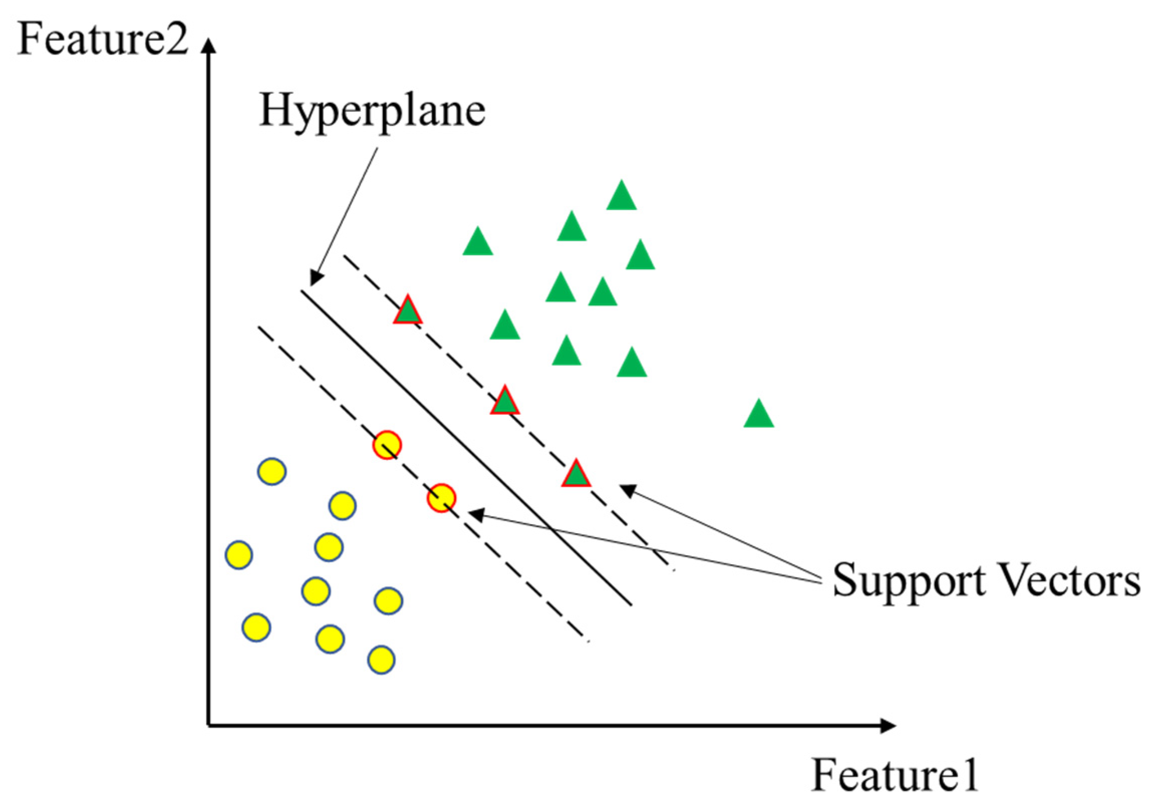
3.2.1. Support Vector Machine

Support vector machine (SVM) theory is proposed by Vapnik [28]. Generally speaking, the support vector machine is a classifier. For the two groups of marked vectors, an optimal segmentation hypersurface is given to divide the two groups of vectors into two sides so that the vector closest to the hyperplane in the two groups of vectors (the so-called support vector) is as far away from the hyperplane as possible. Figure 2 shows the schematic diagram of SVM.
For a data set, d a t a = { ( x 1 , y 1 ) , ( x 2 , y 2 ) , , ( x n , y n ) } , where x i R n , y i { + 1 , 1 } . It can be specifically described as the following problem of finding the conditional maximum value:
{ min a { 1 2 i = 1 m j = 1 m a i a j y i y j ϕ ( x i ) T ϕ ( x j ) i = 1 m a i } j = 1 m a i y i = 0 0 a i C i = 1 , 2 , , m
The above problem involves the vector inner product mapped to a high-dimensional space, that is, the calculation of ϕ ( x i ) T ϕ ( x j ) . Therefore, it is necessary to introduce kernel function K(x,z). This paper employs the Gaussian kernel function:
K ( x , z ) = exp ( x z 2 2 σ 2 )
Besides, LIBSVM tools [29] provide support for the calculation.

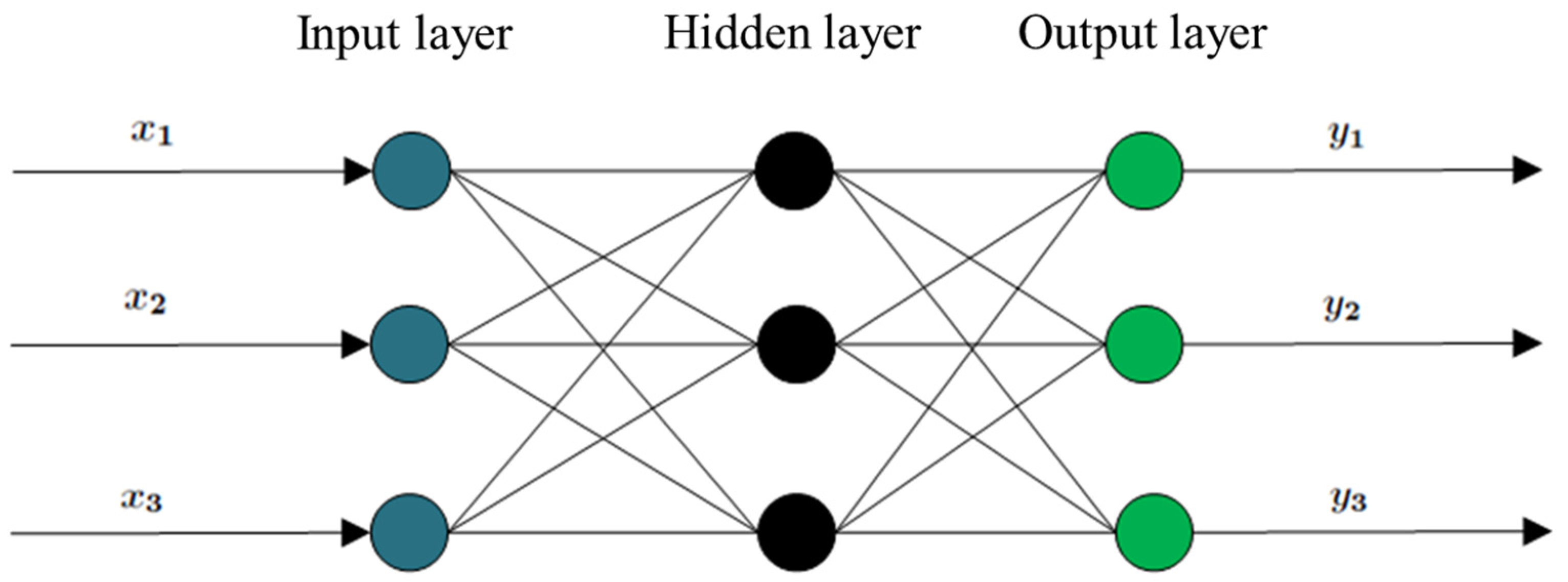
3.2.2. BP Neural Network

BP (Back Propagation) neural network is a multilayer feedforward neural network trained according to the error backpropagation algorithm, which is one of the most widely used neural network models. The process of BP neural network is mainly divided into two stages. The first stage is the forward propagation of the signal, from the input layer to the hidden layer, and finally to the output layer. The second stage is the back-propagation of error, from the output layer to the hidden layer, and finally to the input layer, adjusting the weight and offset from the hidden layer to the output layer and from the input layer to the hidden layer. Figure 3 shows the schematic diagram of a BP neural network.

4. Results and Discussion

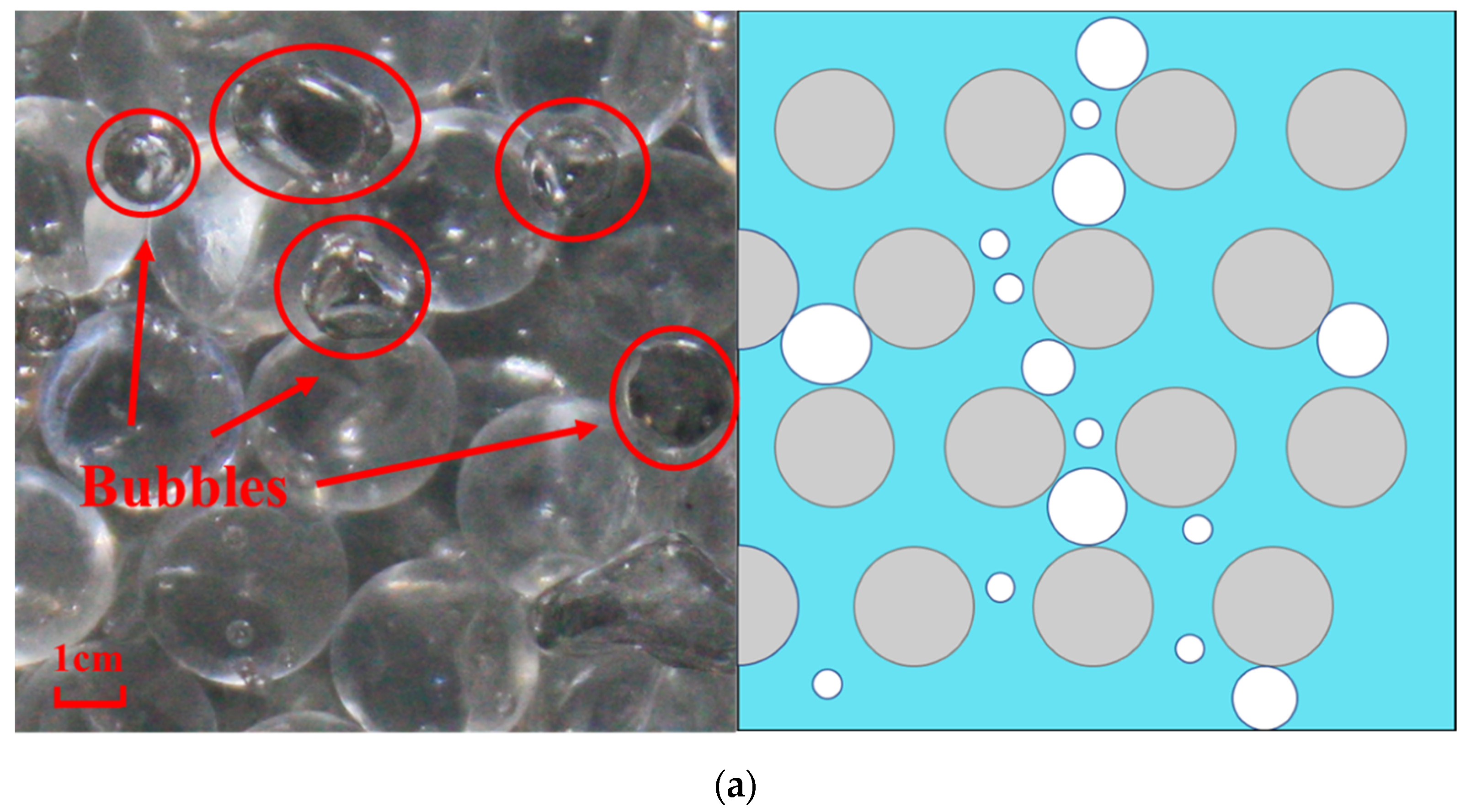
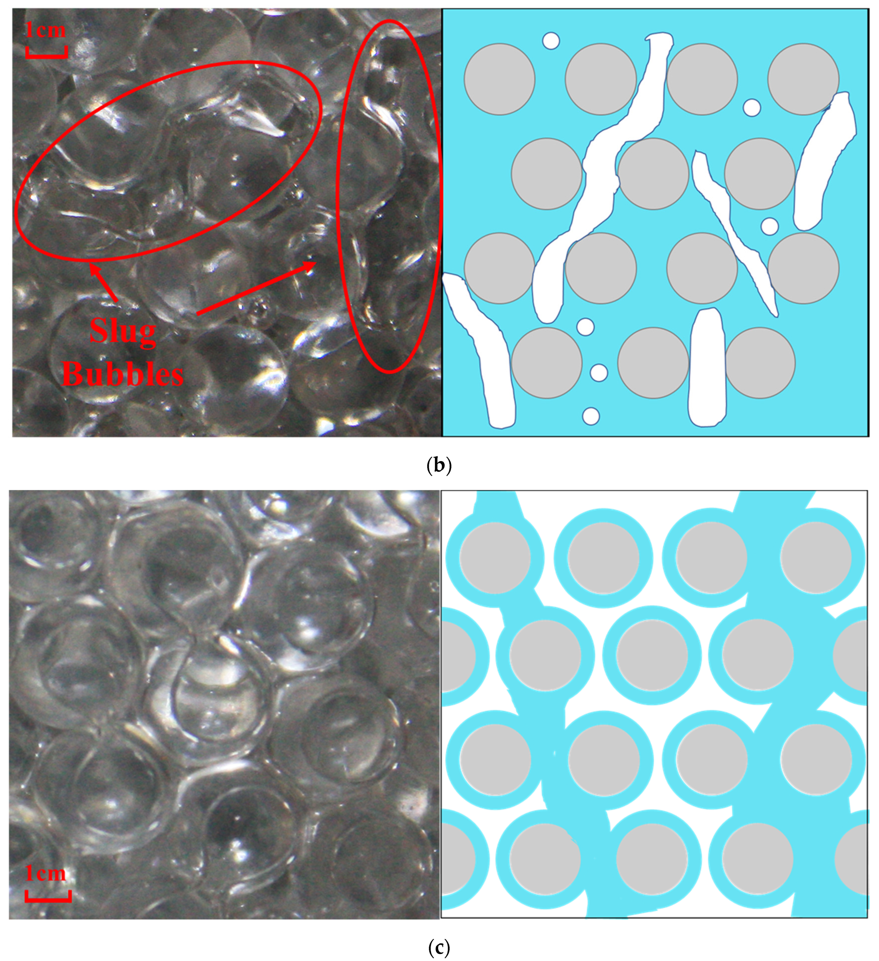
4.1. Experiment Results

In this study, different flow patterns in a porous bed are recorded by changing the gas flow rate while the liquid flow rate is fixed. During this process, bubbly flow, slug flow, annular flow, and the transition flow patterns among them are observed. The photos and diagrams of typical flow patterns are shown in Figure 4. At first, the gas flow rate is lower. At this time, the gas phase is scattered between the pores of the porous media bed in the form of small bubbles. With the continuous increase in gas flow rate, the number and volume of bubbles increase, and the flow pattern begins to transition to slug flow. When the flow pattern is completely transformed into slug flow, it can be seen that the bubbles between adjacent pores are connected to form irregular gas slugs, as shown in Figure 4b. In the whole experimental section, such gas slugs can be seen everywhere. As the gas flow rate further increases, the gas slugs are connected to form larger gas slugs, and the flow pattern transitions to annular flow. For a typical annular flow, the liquid is attached to the surface of particles and pipe walls in the form of a liquid film, and the gas flows rapidly through the gap between these liquid films, as shown in Figure 4c. It is worth mentioning that in porous beds with particle diameters of 1.5 mm and 6 mm, three typical flow patterns cannot be completely observed within the current working conditions due to the limitation of pore size. Bubbly flow cannot be observed in a porous bed with a particle diameter of 1.5 mm. For a porous bed with a particle diameter of 6 mm, annular flow cannot be observed. Only in the porous bed with a particle diameter of 3 mm are bubbly flow, slug flow, and annular flow are observed at the same time.
Figure 5 shows the diagram of differential pressure signals of typical flow patterns in porous beds with different particle diameters. As shown in Figure 5a,b, the differential pressure signals of bubbly flow in two porous beds fluctuate around 4.5 kPa, and the fluctuation ranges are about 1 kPa. The difference in particle diameter does not lead to an obvious difference between differential pressure signals. For slug flow, it can be seen from Figure 5c–e that there is a great difference between the differential pressure signals of bubbly flow and that of slug flow. The differential pressure signals of slug flow in porous beds with particle diameters of 3 mm and 1.5 mm fluctuate up and down around 5 kPa, and the fluctuation ranges can reach about 2 kPa, which is larger than that of bubbly flow. As for the differential pressure signal of slug flow in a porous bed with a particle diameter of 6 mm, although its fluctuation range is small, which is about 1.5 kPa. The average of the signal is around 3.5 kpa at this time, which is significantly smaller than 4.5 kPa of bubbly flow and 5 kPa of slug flow in the other two porous beds. By observing differential pressure signals of annular flow in Figure 5f,g, it can be found that the average value of the differential pressure signals is increased, both greater than 5 kPa. For the porous bed with a particle diameter of 3 mm, the fluctuation range of the differential pressure signal of annular flow is smaller than that of the slug flow.
In general, it can be found that there are certain differences in the features of differential pressure signals of different flow patterns, such as the mean value, dispersion degree, and so on. The features of these typical flow patterns are extracted, quantified, and classified, and then the unknown flow patterns can be classified and recognized through these features. The next section will introduce how to use time domain analysis and EMD methods to extract and quantify the characteristic parameters of differential pressure signals.

4.2. Feature Extraction

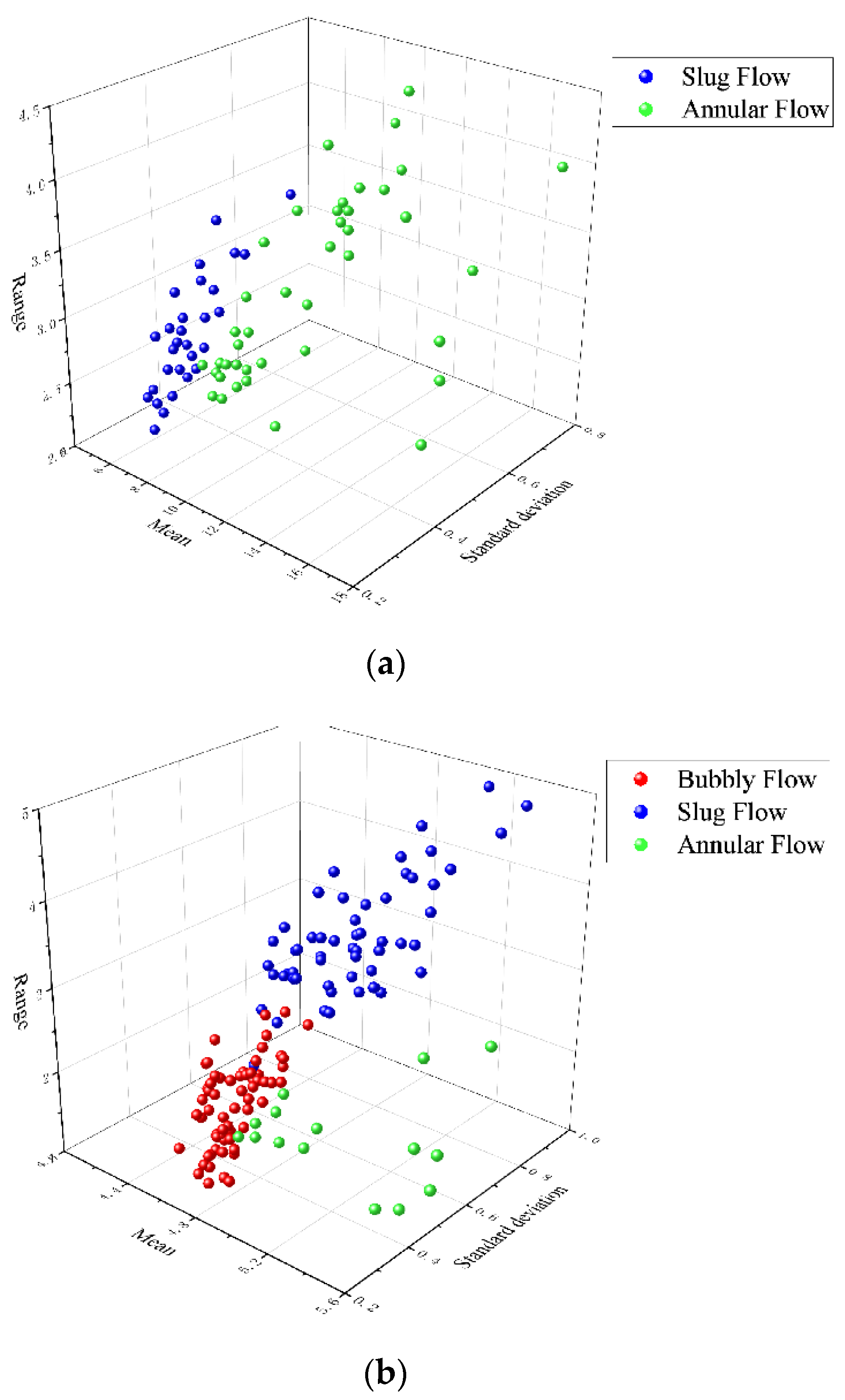
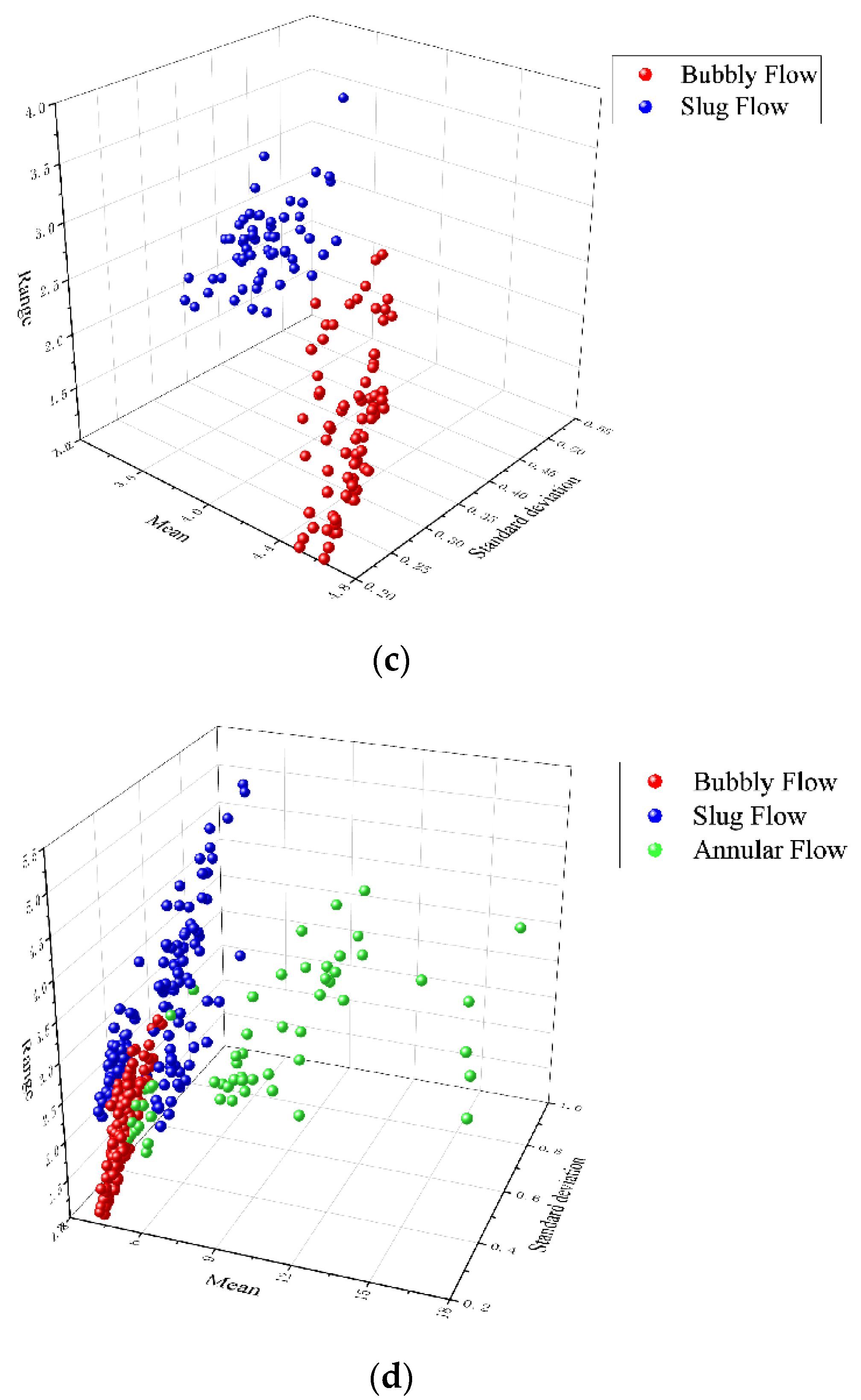
4.2.1. Time Domain Feature Extraction

According to Equations (1)–(3), three time domain parameters (average value, standard deviation, and range) corresponding to each group of data are obtained. The average reflects the concentration trend of the differential pressure signal, the standard deviation reflects the dispersion degree of the differential pressure signal, and the range quantifies the fluctuation range of the differential pressure signal. After sorting out the calculation results, the time domain characteristic distributions of different flow patterns in porous beds with different particle diameters are obtained, as shown in Figure 6.
It can be seen from Figure 6a that there is an obvious boundary between the slug flow and annular flow in a porous bed with a particle diameter of 1.5 mm. Figure 6b shows that in a porous bed with a particle diameter of 3 mm, a few data points of slug flow and bubble flow overlap in the time domain distribution. In Figure 6c, it can be seen that in the porous bed with a particle diameter of 6 mm, there is also an obvious boundary between the distribution of bubble flow and slug flow data in the time domain. Nevertheless, it can be found from Figure 6d that when the influence of particle diameter of porous media bed is not considered, there will be a lot of overlap in the distribution of time domain characteristics of different flow patterns, which indicates that particle diameter is also one of the important parameters affecting classification, and the influence of particle diameter cannot be ignored.
In order to better analyze the distribution of time domain characteristics, the distribution range and median of time domain characteristic parameters of different flow patterns are counted, and the calculation results are shown in Table 2.
It can be seen from the Table 2 that for the porous bed with a particle diameter of 1.5 mm, the average value of the differential pressure signal of the slug flow is 5.74–7.05 kPa, and that of the annular flow is greater than 8.02 kPa. Therefore, the data with the average value of the differential pressure signal falling within these ranges can be directly distinguished between the slug flow and the annular flow in the porous bed with a particle diameter of 1.5 mm. Similarly, in the porous media bed with a particle diameter of 6 mm, the average value of the differential pressure signal can also be directly used to distinguish bubbly flow and slug flow (bubbly flow is 4.11–4.76 kPa, slug flow is 3.38–3.97 kPa). However, it should be considered that the average value of differential pressure signal alone cannot distinguish all the flow patterns. Firstly, in a porous media bed with a particle diameter of 3 mm, there is a range of overlap between the characteristic parameters of different flow patterns. Secondly, for porous media beds with particle diameters of 1.5 and 6 mm, it is also difficult to distinguish data that are between two ranges (for example, the average value of differential pressure signal is within 7.05–8.02 kPa) through the judgment of researchers. This is why multiple parameters rather than a single parameter are selected to judge the flow pattern. To solve the above problems, new features (EMD energy spectrum) are introduced to provide a more judgment basis. At the same time, machine learning technology is employed to identify and classify different flow patterns from a mathematical point of view.

4.2.2. Time-Frequency Feature Extraction

EMD has been briefly introduced in Section 3.1.2. In this section, the differential pressure signals of different flow patterns are decomposed to obtain the IMF components of the signal; the decomposition results are shown in Figure 7.
As can be seen in Figure 7, most of the IMF3 of slug flow is close to zero, which is obviously different from that of bubbly flow and annular flow. Similarly, the IMF4 of bubbly flow is also very different from that of slug flow and annular flow, not only in forms but also in amplitude. Moreover, for IMF6, IMF7, there are also differences in the amplitudes of modal functions of different flow patterns. Therefore, using Equations (6) and (7), the EMD energy spectra of different signals are defined and calculated, and the corresponding distribution ranges are obtained. Due to the adaptability of the EMD method, the decomposition levels of different signals are different. Considering that the amplitudes of IMF8 and IMF9 of most signals are very low (energy is very low), in order to unify the results, only the energy of level one–level seven is retained. The calculation results are shown in Table 3, Table 4 and Table 5. It can be seen from Table 3 that the energy proportion of EMD at levels 1–3 is not high, especially from the median point of view; only the bubbly flow in a porous bed with a particle diameter of 6 mm accounts for more than 10% of the energy at level one. It can be seen from Table 4 that the EMD energy of the signal is mainly distributed at levels four, five, and six, especially at level four. As can be seen in Table 5, the difference in EMD energy at level seven between different conditions is large. For example, for the slug flow in the porous bed with particle diameters of 3 mm and 6 mm, the energy proportion may reach more than 40%, while for other conditions, the energy proportion of this level is much lower.
In general, by processing the signal with the EMD method and calculating the corresponding EMD energy spectrum, new parameters that are different from time domain characteristic parameters can be obtained. These new parameters will show different characteristics with different flow patterns, which can be used for the identification of flow patterns. They also provide richer feature vectors as support for the next machine learning classification.

4.3. Machine Learning Identification

In Section 4.2, the time domain characteristics and EMD energy spectrum of differential pressure signals are calculated. After analyzing these characteristics, it can be found that it is difficult to classify and identify all working conditions with a single parameter, and there is often overlap between parameters. The complex characteristics make it difficult for researchers to accurately identify flow patterns through subjective judgment. The development of machine learning technology, especially support vector machine (SVM) technology and neural network technology, provides new ideas and tools for solving these problems. Through SVM technology and neural network technology, the recognition model can be trained by using multi-dimensional feature vectors based on certain mathematical rules. Compared with manual recognition, these mathematical models can quickly and accurately judge the flow pattern according to the input feature vector, which greatly reduces the impact of subjectivity on the results and improves the recognition efficiency. Therefore, this section uses SVM technology and neural network technology to train multiple SVM/neural network identification models with different features and compares the identification ability of these models to evaluate the performance of the two technologies in porous media flow pattern identification.
Samples should be prepared before training. A total of 341 sets of typical flow pattern data are obtained in this experiment, including bubbly flow, slug flow, and annular flow. One part of the data is used as the training set to train the model, and the other part of the data is used as the test set to test the identification ability of the model. The details are shown in Table 6.
The vector including time domain features and EMD energy spectrum is constructed. Considering the important influence of particle diameter on the characteristics, the particle diameter is also included in the vector. The dimension n of the vector should not be too large, which is limited by the number of training sets. In this paper, n < 8 (2n < 188). Therefore, the final vector is composed of three time domain characteristic parameters, three levels of EMD energy ratio, and one particle diameter. From large to small, two kinds of vectors are constructed, which will lead to two different SVM models. One vector includes four, five, and six levels and the other one includes one, two, and seven levels. Examples of vectors are shown in Table 7.
The SVM models are trained with the prepared vectors. In this paper, the k-CV method [30] combined with the grid search method is used to obtain two key parameters (the penalty factor C and the kernel function parameter g), which are important to ensure the accuracy of SVM models. Table 8 shows the identification results of the two SVM models.
In general, the identification ability of the SVM-1 model is better than that of the SVM-2 model. The identification ability of slug flow and annular flow of SVM-1 model is better than that of the SVM-2 model. However, its bubbly flow identification ability is worse than that of the SVM-2 model, but this gap is not very obvious.
In addition to the SVM model, the neural network flow pattern identification model is also trained based on BP neural network technology. In this paper, BP neural network includes one input layer (7 neurons, corresponding to seven features of a vector), one intermediate layer (12 neurons), and one output layer (3 neurons, corresponding to labels of three flow patterns). The same training set and test set as SVM models are selected, which can help evaluate the identification ability of the two methods. The training results are shown in Table 9.
As shown in Table 9, the identification ability of different BP network models varies greatly. The BP-1 model has the best identification ability, which is not only better than the BP-2 model but also better than SVM-1 and SVM-2 models. The identification ability of the BP-2 model is the worst of the four models. Moreover, the models containing one, two, and seven levels of EMD energy perform worse than the models containing four, five, and six levels of EMD energy.
Next, consider further improving the identification ability of flow patterns. The idea of bagging technology in integrated learning technology is introduced. That is, train multiple models at the same time, let these models vote on the results, and determine the final results according to the voting results. In this study, four models are trained. If all the models participate in the voting, there may be a tie vote. Due to the poor performance of BP-2, its results may mislead the correct results. Therefore, SVM-1, SVM-2, and BP-1 were selected to form an integrated model. The identification process is shown in Figure 8, moreover, considering the special situation (bubble flow: annular flow: slug flow, 1:1:1). Since the BP-1 model performed best among the three models, it is considered that the final result of BP-1 model will prevail when the conflict occurs. Table 10 shows the identification results of an integrated model. It can be seen that the integrated model further improves identification ability based on the original models. The test data of bubbly flow and annular flow have been correctly identified, and only two groups of slug flow data have not been correctly identified.

5. Conclusions

In this paper, a method based on feature extraction and machine learning is proposed to identify the two-phase flow patterns in porous media, which provides a new idea for the development of flow pattern identification methods in porous media in the fields of the chemical industry, agriculture, petroleum, and nuclear engineering. The differential pressure signals of two phase flow in the porous media packed with particles are collected through visual experiments. The time domain characteristic parameters and EMD energy spectrum are extracted. After that, a variety of flow pattern identification models based on machine learning technology are trained. An integrated flow pattern identification model with high accuracy is finally obtained based on integrated identification technology. The main conclusions are as follows:
(1)
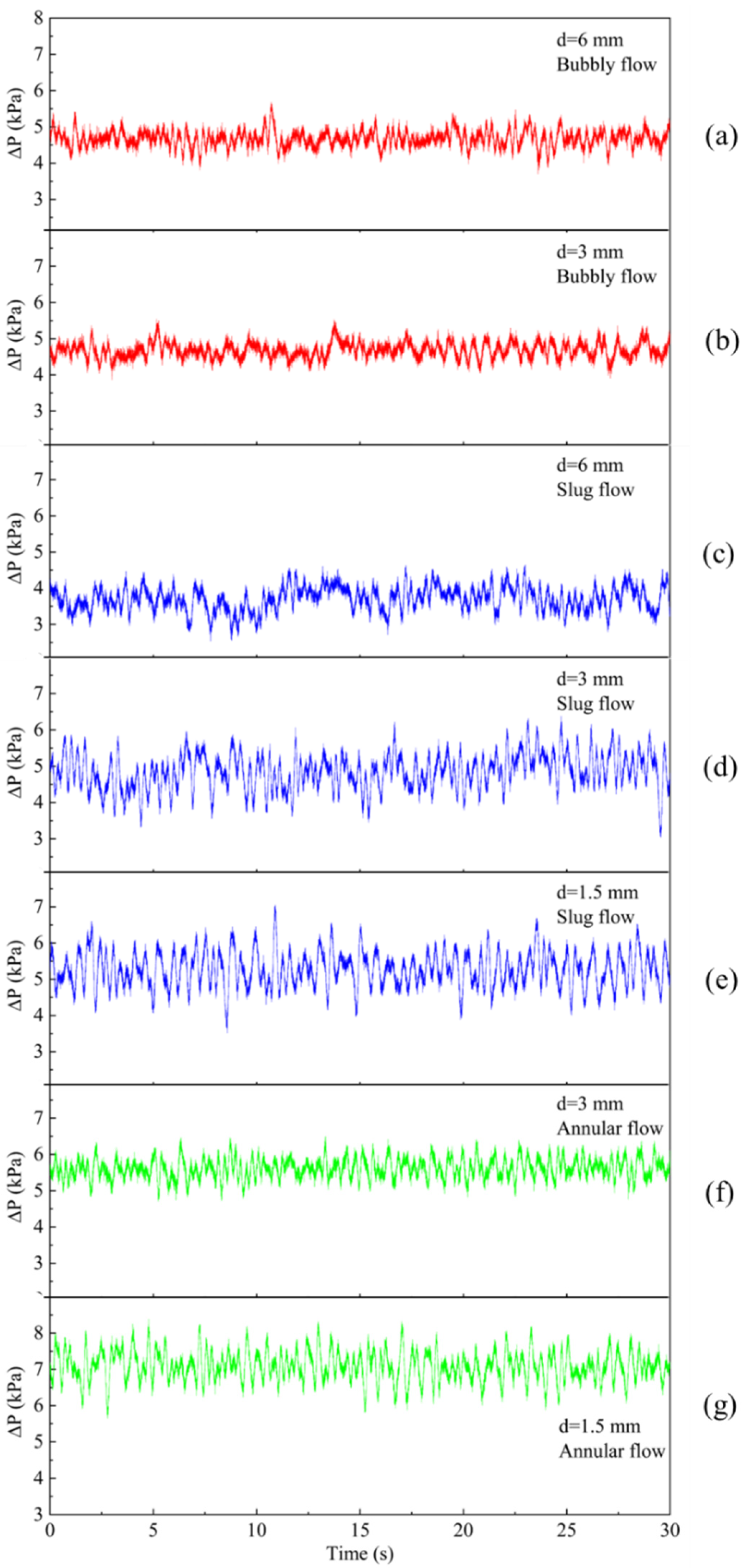
There are differences between the average values of differential pressure signals of different flow patterns. For a porous bed with a particle diameter of 1.5 mm, the boundary between slug flow and annular flow is 8 kPa. For a porous bed with a particle diameter of 3 mm, the distribution range of average differential pressure of different flow patterns overlaps. For a porous bed with a particle diameter of 6 mm, the boundary between bubbly flow and slug flow is 4 kPa. For other parameters, the overlapping area between different flow patterns is larger, and it is difficult to distinguish the flow patterns only by manual identification. It is necessary to introduce machine learning technology.
(2)
The BP-1 model based on BP neural network technology has the best identification ability among single models, with an accuracy of 96.08%. However, another BP-2 model based on different levels of EMD energy has the worst identification ability. Its accuracy is only 91.5%. The identification ability of the two models SVM-1 and SVM-2 trained by SVM technology is close, since the accuracies of them are 94.77%, and 93.4%, respectively. In this study, the two neural network models have the highest and lowest recognition accuracy. Although the SVM model is lower than the optimal neural network model in recognition accuracy, the recognition ability of the two models is closer. SVM technology is more stable than BP neural network technology.
(3)
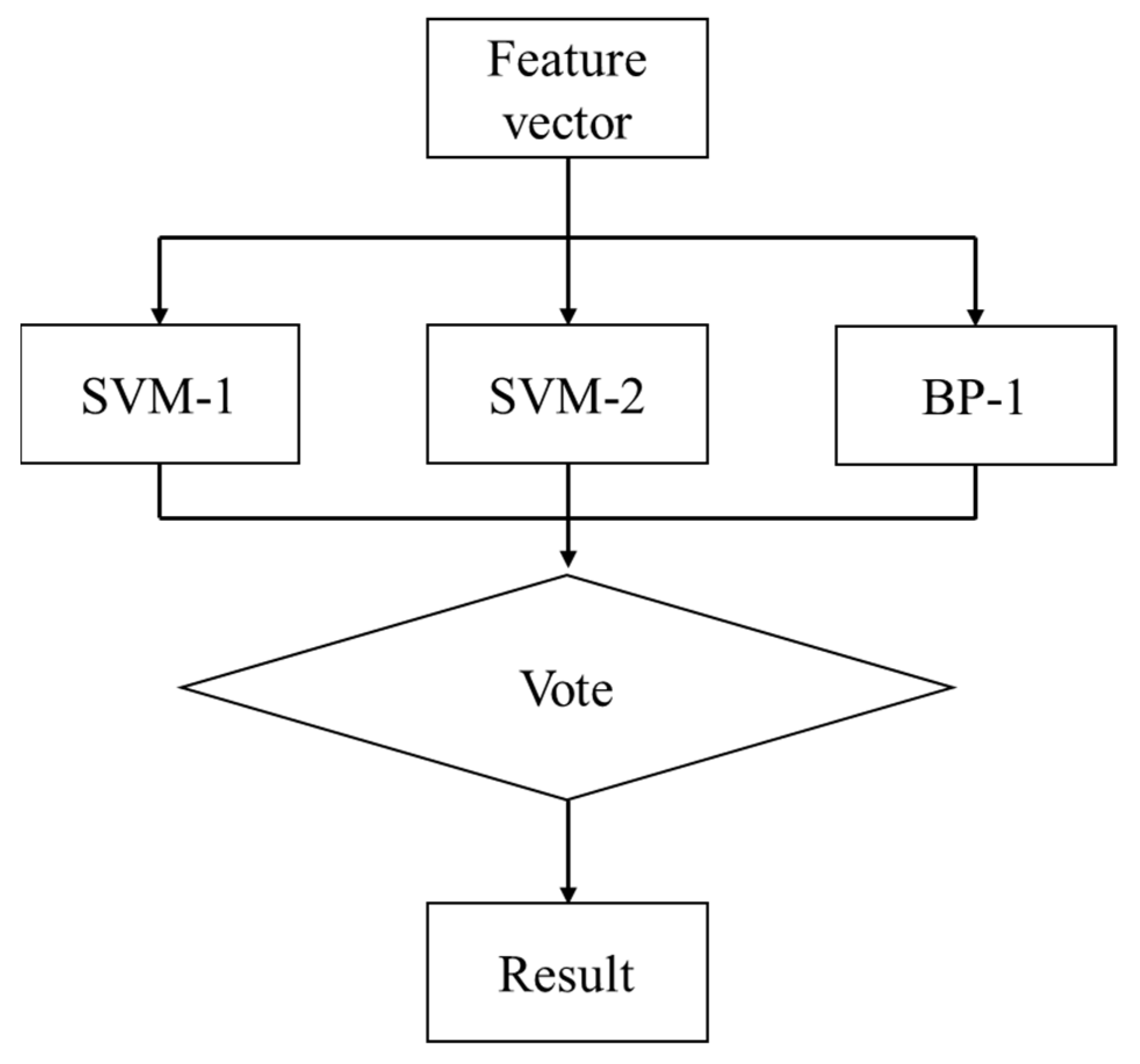
By integrating several high-quality models, the integrated model can further improve the ability of flow pattern identification on the basis of the original models. The identification accuracy increased from 94.77% to 98.04%. This behavior will increase the total calculation time because it takes time to train each model. The total time is approximately equal to the sum of the time needed to train the three models, respectively. Users can consider comprehensively according to the requirements for accuracy and timeliness. Moreover, poor quality models will reduce the identification ability of integrated models.

Author Contributions

Conceptualization, L.L.; Data curation, X.L. and J.Z.; Formal analysis, W.W., H.Z. and J.Z.; Investigation, X.L. and L.L.; Methodology, X.L., L.L. and J.Z.; Software, W.W. and H.Z.; Visualization, W.W. and H.Z.; Writing—original draft, X.L.; Writing—review & editing, L.L. All authors have read and agreed to the published version of the manuscript.

Funding

This research received no external funding.

Conflicts of Interest

The authors declare no conflict of interest.

Nomenclature

aapproximation coefficient, 1
bConstant term of hyperplane equation,1
CCrest factor, 1
Elocal energy density, 1
Jflow rate, mm/s
Kkernel function
Ppower spectral density, kPa2/Hz
RRange value
ssignal
SStandard deviation
ttime
xCoordinates
yCoordinates
zCoordinates
Фscaling function
Subscripts
ggas
iunit number
junit number
kunit number
munit number
maxmaximum
minminimum
Munit number
RRange value
SStandard deviation
Acronyms
BPBack propagation
EMDEmpirical mode decomposition
IMFIntrinsic mode function
SVMsupport vector machine

References

  1. Ma, W.; Yuan, Y.; Sehgal, B.R. In-Vessel Melt Retention of Pressurized Water Reactors: Historical Review and Future Research Needs. Engineering 2016, 2, 103–111. [Google Scholar] [CrossRef]
  2. Hu, B.; Gu, Z.; Zhou, C.; Wang, L.; Huang, C.; Su, J. Investigation of the Effect of Capillary Barrier on Water–Oil Movement in Water Flooding. Appl. Sci. 2022, 12, 6285. [Google Scholar] [CrossRef]
  3. Kulli, B. Visualizing soil compaction based on flow pattern analysis. Soil Tillage Res. 2003, 70, 29–40. [Google Scholar] [CrossRef]
  4. Zhang, C.; Jiao, W.; Liu, Y.; Qi, G.; Yuan, Z.; Zhang, Q. CFD Simulation of Dry Pressure Drop in a Cross-Flow Rotating Packed Bed. Appl. Sci. 2021, 11, 10099. [Google Scholar] [CrossRef]
  5. Yao, T.; Wu, Q.; Liu, Z.; Zou, S.; Xu, Q.; Guo, L. Experimental investigation on mitigation of severe slugging in pipeline-riser system by quasi-plane helical pipe device. Exp. Therm. Fluid Sci. 2019, 102, 189–204. [Google Scholar] [CrossRef]
  6. Tosun, G. A study of cocurrent downflow of nonfoaming gas-liquid systems in a packed bed. 1. Flow regimes: Search for a generalized flow map. Ind. Eng. Chem. Process Des. Dev. 1984, 23, 29–35. [Google Scholar] [CrossRef]
  7. Tung, V.; Dhir, V. A hydrodynamic model for two-phase flow through porous media. Int. J. Multiph. Flow 1988, 14, 47–65. [Google Scholar] [CrossRef]
  8. Xu, G.; Zhang, X.; Sun, Z.; Ruan, J.; He, B. Flow patterns and transition criteria in boiling water-cooled packed bed reactors. Prog. Nucl. Energy 2018, 108, 214–221. [Google Scholar] [CrossRef]
  9. Shaban, H.; Tavoularis, S. Identification of flow regime in vertical upward air–water pipe flow using differential pressure signals and elastic maps. Int. J. Multiph. Flow 2014, 61, 62–72. [Google Scholar] [CrossRef]
  10. Wu, B.; Ribeiro, A.S.; Firouzi, M.; Rufford, T.E.; Towler, B. Use of pressure signal analysis to characterise counter-current two-phase flow regimes in annuli. Chem. Eng. Res. Des. 2020, 153, 547–561. [Google Scholar] [CrossRef]
  11. Vieira, S.C.; van der Geest, C.; Fabro, A.; de Castro, M.S.; Bannwart, A.C. Intermittent slug flow identification and characterization from pressure signature. Mech. Syst. Signal Process. 2021, 148, 107148. [Google Scholar] [CrossRef]
  12. Guo, W.; Liu, C.; Wang, L. Temperature fluctuation on pipe wall induced by gas–liquid flow and its application in flow pattern identification. Chem. Eng. Sci. 2021, 237, 116568. [Google Scholar] [CrossRef]
  13. Huang, N.E.; Shen, Z.; Long, S.R.; Wu, M.C.; Shih, H.H.; Zheng, Q.; Yen, N.-C.; Tung, C.C.; Liu, H.H. The empirical mode decomposition and the Hilbert spectrum for nonlinear and non-stationary time series analysis. Proc. R. Soc. Lond. Ser. A Math. Phys. Eng. Sci. 1998, 454, 903–995. [Google Scholar] [CrossRef]
  14. Matsui, G. Identification of flow regimes in vertical gas-liquid two-phase flow using differential pressure fluctuations. Int. J. Multiph. Flow 1984, 10, 711–719. [Google Scholar] [CrossRef]
  15. Elperin, T.; Klochko, M. Flow regime identification in a two-phase flow using wavelet transform. Exp. Fluids 2002, 32, 674–682. [Google Scholar] [CrossRef]
  16. dos Reis, E.; Goldstein, L., Jr. Characterization of slug flows in horizontal piping by signal analysis from a capacitive probe. Flow Meas. Instrum. 2010, 21, 347–355. [Google Scholar] [CrossRef]
  17. Li, X.; Wei, T.; Wang, D.; Hu, H.; Kong, L.; Xiang, W. Study of gas–liquid two-phase flow patterns of self-excited dust scrubbers. Chem. Eng. Sci. 2016, 151, 79–92. [Google Scholar] [CrossRef]
  18. Khorasani, M.; Ghasemi, A.; Leary, M.; Sharabian, E.; Cordova, L.; Gibson, I.; Downing, D.; Bateman, S.; Brandt, M.; Rolfe, B. The effect of absorption ratio on meltpool features in laser-based powder bed fusion of IN718. Opt. Laser Technol. 2022, 153, 108263. [Google Scholar] [CrossRef]
  19. Sezer, H.; Tang, J.; Ahsan, A.N.; Kaul, S. Modeling residual thermal stresses in layer-by-layer formation of direct metal laser sintering process for different scanning patterns for 316L stainless steel. Rapid Prototyp. J. 2022. ahead of print. [Google Scholar] [CrossRef]
  20. Rashed, K.; Kafi, A.; Simons, R.; Bateman, S. Fused Filament Fabrication of Nylon 6/66 Copolymer: Parametric Study Com-paring Full Factorial and Taguchi Design of Experiments. Rapid Prototyp. J. 2022, 28, 1111–1128. [Google Scholar] [CrossRef]
  21. Agrawal, R. Sustainable design guidelines for additive manufacturing applications. Rapid Prototyp. J. 2022, 28, 1221–1240. [Google Scholar] [CrossRef]
  22. Liang, F.; Hang, Y.; Yu, H.; Gao, J. Identification of gas-liquid two-phase flow patterns in a horizontal pipe based on ultrasonic echoes and RBF neural network. Flow Meas. Instrum. 2021, 79, 101960. [Google Scholar] [CrossRef]
  23. Pei, S.; Liu, H.; Zhu, Y.; Zhang, C.; Zhao, M.; Fu, G.; Yang, K.; Yuan, Y.; Zhang, C. Identifying Flow Patterns in Water Pipelines Using Complex Network Theory. J. Hydraul. Eng. 2021, 147, 04021019. [Google Scholar] [CrossRef]
  24. Zhang, L.; Wang, H. Identification of oil–gas two-phase flow pattern based on SVM and electrical capacitance tomography technique. Flow Meas. Instrum. 2010, 21, 20–24. [Google Scholar] [CrossRef]
  25. Liu, W.; Tan, C.; Dong, F. Doppler spectrum analysis and flow pattern identification of oil-water two-phase flow using dual-modality sensor. Flow Meas. Instrum. 2021, 77, 101861. [Google Scholar] [CrossRef]
  26. Ambrosio, J.D.S.; Lazzaretti, A.E.; Pipa, D.R.; da Silva, M.J. Two-phase flow pattern classification based on void fraction time series and machine learning. Flow Meas. Instrum. 2021, 83, 102084. [Google Scholar] [CrossRef]
  27. Li, L.; Zou, X.; Wang, H.; Zhang, S.; Wang, K. Investigations on two-phase flow resistances and its model modifications in a packed bed. Int. J. Multiph. Flow 2018, 101, 24–34. [Google Scholar] [CrossRef]
  28. Vapnik, V.N. An overview of statistical learning theory. IEEE Trans. Neural Netw. 1999, 10, 988–999. [Google Scholar] [CrossRef]
  29. Chang, C.; Lin, C. LIBSVM: A Library for Support Vector Machines. ACM Trans. Intell. Syst. Technol. 2011, 2, 1–27. [Google Scholar] [CrossRef]
  30. Rodriguez, J.D.; Perez, A.; Lozano, J.A. Sensitivity Analysis of k-Fold Cross Validation in Prediction Error Estimation. IEEE Trans. Pattern Anal. Mach. Intell. 2010, 32, 569–575. [Google Scholar] [CrossRef]
Figure 1. Diagram of DEBECO-LT and test section. 1—Stainless steel wire mesh, 2—Fittingflange, 3—Connecting pipe, 4—Gas–liquid separator, 5—Differential pressure transmitter, 6—Test section.
Applsci 12 08575 g001
Figure 2. The classification principle of SVM.
Applsci 12 08575 g002
Figure 3. Schematic diagram of BP neural network.
Applsci 12 08575 g003
Figure 4. Photos and diagrams of typical flow patterns. (a). Photo and diagram of bubbly flow. (b). Photo and diagram of slug flow. (c). Photo and diagram of annular flow.
Applsci 12 08575 g004aApplsci 12 08575 g004b
Figure 5. Diagram of differential pressure signals of typical flow patterns in different porous beds. (a). d = 6 mm, bubbly flow. (b). d = 3 mm, bubbly flow. (c). d = 6 mm, slug flow. (d). d = 3 mm, slug flow. (e). d = 1.5 mm, slug flow. (f). d = 3 mm, annular flow. (g). d = 1.5 mm, annular flow.
Applsci 12 08575 g005
Figure 6. Diagram of time domain characteristic parameter distribution. (a). Time domain characteristic parameter distribution in porous bed with a particle diameter of 1.5 mm. (b). Time domain characteristic parameter distribution in porous bed with a particle diameter of 3 mm. (c). Time domain characteristic parameter distribution in porous bed with a particle diameter of 6 mm. (d). Time domain characteristic parameter distribution in all porous beds.
Applsci 12 08575 g006aApplsci 12 08575 g006b
Figure 7. IMF components of different flow patterns.
Applsci 12 08575 g007
Figure 8. Diagram of integrated model.
Applsci 12 08575 g008
Table 1. Details of experiment setup.
Particle Sizes (mm)PorositySuperficial Velocity Reynolds Number
Water (mm/s)Gas (m/s)WaterGas
1.50.3910.59~1.170.005–0.441.13–2.261.87–97.93
30.3850.29~1.170.005–0.441.21–5.121.98–161.92
60.40.29~1.170.005–0.442.31–10.013.65–327.55
Table 2. Distribution of time domain parameters of flow patterns.
Particle DiameterQuartileBubbly FlowSlug FlowAnnular Flow
mSRmSRmSR
1.5 mmmin 5.740.282.088.020.332.35
median6.130.382.6510.270.463.11
max7.050.603.5017.480.744.40
3 mmmin4.650.211.474.730.382.434.930.271.79
median4.850.302.185.050.543.645.270.292.26
max5.010.443.015.490.865.085.880.513.25
6 mmmin4.110.171.263.380.311.99
median4.600.261.913.610.372.52
max4.760.402.713.970.503.51
allmin4.110.171.263.380.281.994.930.271.79
median4.700.281.984.910.412.799.000.402.72
max5.010.443.017.050.865.0817.480.744.40
Table 3. Distributions of EMD energy spectrum on levels 1–3.
Particle DiameterQuartileBubbly FlowSlug FlowAnnular Flow
Level 1Level 2Level 3Level 1Level 2Level 3Level 1Level 2Level 3
1.5 mmmin 2.38%1.15%0.35%1.46%0.74%0.29%
median5.50%2.55%0.86%3.83%1.81%3.23%
max9.06%4.37%8.97%7.61%3.58%30.81%
3 mmmin3.05%1.53%0.48%1.05%0.54%0.21%3.07%1.47%0.40%
median7.55%3.53%0.97%2.48%1.23%1.94%8.84%4.15%1.53%
max16.77%7.71%7.02%5.01%2.31%12.42%12.24%5.88%5.96%
6 mmmin4.41%2.34%0.78%2.81%1.51%0.56%
median10.36%5.25%1.46%5.24%2.86%0.90%
max26.74%12.76%3.55%7.50%4.04%2.29%
Table 4. Distributions of EMD energy spectrum on levels 4–6.
Particle DiameterQuartileBubbly FlowSlug FlowAnnular Flow
Level 4Level 5Level 6Level 4Level 5Level 6Level 4Level 5Level 6
1.5 mmmin 12.89%5.62%4.17%14.67%8.20%3.18%
median41.20%15.76%8.70%49.53%19.06%6.34%
max54.80%28.95%15.18%63.68%32.43%15.24%
3 mmmin4.20%7.78%6.28%18.91%8.80%3.56%17.22%9.26%2.95%
median27.93%23.54%15.71%38.60%16.42%9.37%47.36%25.62%5.35%
max41.96%36.65%30.57%54.29%31.79%23.24%53.11%36.10%9.27%
6 mmmin15.70%11.03%6.56%8.97%10.90%5.52%
median32.78%22.00%13.26%22.36%20.97%15.36%
max46.04%37.71%27.43%32.97%33.70%31.20%
Table 5. Distributions of EMD energy spectrum on level 7.
Particle DiameterQuartileBubbly FlowSlug FlowAnnular Flow
Level 7Level 7Level 7
1.5 mmmin 2.80%0.52%
median7.88%3.38%
max15.33%13.96%
3 mmmin3.71%1.40%1.19%
median10.94%12.61%2.13%
max24.44%46.50%9.21%
6 mmmin1.65%3.51%
median5.02%14.75%
max12.52%43.14%
Table 6. The number of samples of different flow patterns.
Flow Pattern Data Sets
TrainTestTotal
Bubbly7763140
Slug8065145
Annular312556
total188153341
Table 7. Examples of vectors with different features.
Vector TypeParametersLabelFlow Pattern
mSRLevel 4Level 5Level 6dp
Vector-14.860.221.6412.41%16.73%30.57%31Bubbly
3.960.392.6922.55%24.26%15.26%62Slug
8.740.342.7155.92%12.33%9.04%1.53Annular
mSRLevel 1Level 2Level 7dp
Vector-24.860.221.6416.24%7.14%12.95%31Bubbly
3.960.392.693.60%1.95%13.84%62Slug
9.080.342.726.23%2.85%2.90%1.53Annular
Table 8. The identification results of SVM models.
SVM ModelFlow PatternCorrect IdentificationTotal NumberAccuracy
SVM-1Bubbly 606395.24%
Slug626595.38%
Annular 232592.00%
Overall14515394.77%
SVM-2Bubbly 616396.83%
Slug 606592.31%
Annular 222588.00%
Overall14315393.46%
Table 9. The identification results of BP-network models.
BP-Network ModelFlow PatternCorrect IdentificationTotal NumberAccuracy
BP-1Bubbly 616396.83%
Slug636596.92%
Annular 232592.00%
Overall14715396.08%
BP-2Bubbly 586392.06%
Slug 616593.85%
Annular 212584.00%
Overall14015391.50%
Table 10. Identification results of integrated model.
Flow PatternCorrect IdentificationTotal NumberAccuracy
Integrated modelBubbly6363100.00%
Slug636596.92%
Annular2525100.00%
Overall15115398.69%
Publisher’s Note: MDPI stays neutral with regard to jurisdictional claims in published maps and institutional affiliations.

