
Unsupervised and Supervised Feature Selection for Incomplete Data via L2,1-Norm and Reconstruction Error Minimization


College of Communications Engineering, Army Engineering University of PLA, Nanjing 210007, China
*
Author to whom correspondence should be addressed.
Appl. Sci. 2022, 12(17), 8752; https://0-doi-org.brum.beds.ac.uk/10.3390/app12178752
Submission received: 20 July 2022
/
Revised: 25 August 2022
/
Accepted: 26 August 2022
/
Published: 31 August 2022
(This article belongs to the Special Issue Advances in Artificial Intelligence: Machine Learning, Data Mining and Data Sciences)
Abstract
:Feature selection has been widely used in machine learning and data mining since it can alleviate the burden of the so-called curse of dimensionality of high-dimensional data. However, in previous works, researchers have designed feature selection methods with the assumption that all the information from a data set can be observed. In this paper, we propose unsupervised and supervised feature selection methods for use with incomplete data, further introducing an L2,1 norm and a reconstruction error minimization method. Specifically, the proposed feature selection objective functions take advantage of an indicator matrix reflecting unobserved information in incomplete data sets, and we present pairwise constraints, minimizing the L2,1-norm-robust loss functionand performing error reconstruction simultaneously. Furthermore, we derive two alternative iterative algorithms to effectively optimize the proposed objective functions and the convergence of the proposed algorithms is proven theoretically. Extensive experimental studies were performed on both real and synthetic incomplete data sets to demonstrate the performance of the proposed methods.
1. Introduction
Due to the rapid progress in the development of information technology in many fields, such as pattern recognition, machine learning, computer vision and data mining, data are usually represented by high-dimensional feature vectors. High-dimensional feature vectors suffer from a high processing time and large space requirements. In addition, data sets with high-dimensional representations usually contain noise features, which may degrade the performance of data mining and pattern recognition tasks. To solve this problem, feature selection [1,2,3,4,5,6,7,8] techniques have been proposed in order to select feature subsets from high-dimensional feature vectors to achieve efficient and accurate data representations.
According to the availability of data labels, feature selection algorithms can be roughly divided into two categories: supervised feature selection (SFS) and unsupervised feature selection (UFS). SFS [1,2,3] algorithms identify the relevant features in order to best achieve the goal of the supervised model, whereas UFS [4,5,6,7,8] algorithms are interpretable, since it is usually difficult to obtain the labels of samples in practical applications.
In practical applications, it is challenging to analyze an incomplete data set with unobserved data, such as missing data, although this issueis ubiquitous in industrial data sets [9,10] and has a significant effect on design methodsin many machine learning, computer vision, data mining, and pattern recognition applications. Moreover, most technologies used for data analysis are based on data sets in which all the information can be observed. Therefore, traditional feature selection methods cannot be directly applied to incomplete data sets. In recent years, many strategies have been proposed to remove the influence of missing data by deleting or imputing the unobserved instances, which has enabled the utilization of existing machine learning techniques [9,10,11,12].
An instance-deletion method was proposed for removing the missing instances of a data set, in which only the unbroken instances are applied in the feature selection process. This can cause some useful information from missing instances to be discarded, which may degrade the data analysis performance. Furthermore, the scale of missing instances in the incomplete data is usually so large that the instance-deletion method becomes invalid. Therefore, imputation methods have been proposed to handle these issues, in which the values of missing instances are estimated using the traditional machine learning techniques [11,12], such as the K-nearest neighbor technique (KNN). However, in feature selection with imputation methods, when using all instances, noise or non-useful information may be introduced;thus, a margin-based feature selection method [13] was designed without imputing missing values, in which the uncertainty of each instance was considered.
In this work, the reconstruction of incomplete data is designed as the feature selection criterion, in which the selected feature approximates the original missing instance by means of a weigh matrix.Specifically, we propose unsupervised and supervised feature selection methods for incomplete data by further introducing the L2,1 norm and through reconstruction error minimization. Specifically, the proposed feature selection objective functions take advantage of an indicator matrix for the unobserved information relating to an incomplete data set. We design pairwise constraints, minimizing the L2,1-norm-robust loss function and performing error reconstruction simultaneously.We further derive an alternative iterative algorithm to effectively optimize the proposed objective functions and the convergence of the proposed algorithms is proven theoretically. Consequently, extensive experimental studies were performed on both real and synthetic incomplete data sets to demonstrate the performance of the proposed methods.
This paper is organized as follows. In Section 2, we review the related works. Then, in Section 3, we present the details of our approach, design the pairwise constraints objection function, optimize the proposed objective functions, and prove the convergence. Next, in Section 4, we display the results of extensive experimental studies and compare the performance of our proposed approach with that of other approaches. Finally, Section 5 concludes the paper.
2. Related Work
Several feature selection approaches [1,2,3,4,5,6,7,8] have been introduced in the literature for complete data in recent years. For incomplete data, there are two strategies that are generally used for feature selection: one involves deleting or imputing the unobserved instances to convert the incomplete data set into a complete data set and then performing feature selection; the other involves directly performing feature selection using the incomplete data set. In this section, we review the work related to these two strategies and analyze the differences between them.
2.1. Imputation Methods
A major issue in feature selection using an incomplete data set is that the traditional methods become invalid. A number of works have addressed this issue and presented a two-stage method to select features from incomplete data sets, primarily in which the missing values are imputed or deleted.
A straightforward and simple method of complete case analysis (CCA) was proposed in [14], in which the samples or features containing missing values are deleted. However, this in turn becomes invalid when the proportion of missing instances is high and the total amount is small. Imputation methods are another more intuitive option, and the classic form of this method is mean imputation. The mean imputation method takes the mean value of the observed feature values as the estimated value of the missing values [15]. However, this method reduces the uncertainty of features and the variance. Another imputation method based on statistics is the expectation maximization (EM) imputation method [16], which uses edge distribution of existing data to conduct maximum likelihood estimation method for missing data, which is used to obtain the corresponding imputation value. In recent years, S. Zhang et al. proposed KNN imputation [12], in which the mean value of the nearest neighbor samples was taken as the estimated value of the missing value. An improved k-nearest neighbor imputation method was also proposed to improve the classification accuracy further and achieve a filling effect [17]. J. Stekhoven et al. proposed and evaluated an iterative imputation method (missForest) based on random forest, with the results showing that missForest could successfully handle missing values, particularly in datasets including different types of variables [18].
Recently, the use of deep learning models has been explored for missing-value imputation [19,20,21,22]. Gondara et al. proposed an imputation model based on deep denoising autoencoders for multiple imputation [19]. A probabilistic framework based on deep generative models for missing value imputation was proposed in [20]. Mattei et al. proposed a simple framework for performing approximate maximum likelihood training with an incomplete data set [21].
However, the results of missing value imputation of unobserved information may be non-useful or even noisy [23]. The reason for this is that there is no ground truth for unobserved information, so the correctness of the imputed information cannot be evaluated.
2.2. Unsupervised Feature Selection Methods on Incomplete Data Sets
Since obtaining class label information is difficult in real-world applications, UFS is one of the dimensionality reduction techniques used to handle high-dimensional data.
UFS methods are usually divided into three categories: filter models, wrapper models, and embedded models. The filter model [24] first selects the features of the data set and then trains the classifier, and the feature selection process is independent of the data mining task. Hence, they usually have a lower computational cost. Lapscore [25] is one of the classical filtering methods, which independently calculates the score of each feature according to its ability to retain the internal structure of the original data, and then select the feature with the highest-ranking score.
The wrapper model [26] does not consider the difference of a specific classifier and directly takes the performance of the classifier to be used as the evaluation criterion of the feature subset. In general, the wrapper method can achieve better performance than the filter method but with high computational cost. LVW (Las Vegas wrapper) is a typical encapsulated feature selection method. It uses a random strategy to search subsets within the framework of the Las Vegas method and evaluates feature subsets based on the error of the final classifier.
The embedded model [27] integrates feature selection into the learning model. Since there is no need to evaluate feature subsets, they are more efficient than the wrapper approach. Therefore, many representative embedded methods have emerged continuously. For example, the general framework for sparsity regularization (GSR) [28] is a general sparse embedding model, which can simultaneously perform feature selection and reduce outliers through parameter adjustment. Robust feature selection (RFS) [29] is another typical embedded model of feature selection. The method has proven its effectiveness in reducing the influence of outliers. Regularized self-representation (RSR) [8] is a framework in which every feature is reconstructed from all features using self-representation, and features are selected using L2,1-norm regularization.
The authors of [30] present a method of multicriteria-based feature selection in cost-sensitive data with missing values, using a rough set theory to deal with unobserved information. Shen proposed the HQ-UFS method, whichcan be directly applied to incomplete data sets [23]. The index matrix is used to filter the unobserved information, and the half-quadratic minimization technique is used to make the weight of outliers negligible or even zero, whereas the weight of essential samples is more prominent, thereby reducing the influence of outliers. In [31], an L2,1-norm minimization method for UFS from incomplete data was proposed, with the authors showing that the proposed algorithm can select more accurate features from a large data set and showing an improved clustering effect.
2.3. Supervised Feature Selection Methods on Incomplete Data Sets
In recent years, some researchers have considered the use of SFS on incomplete data sets without preprocessing missing values. Similarly to the use of UFS methods on incomplete data sets, SFS would also require some imputation methods to be implemented prior to the application of existing SFS methods, such as Simba [32] and Relief [33]. In [34], a method for modeling multivariate spatio-temporal data was presented, in which the missing values are estimated first, and then the feature selection procedure is applied. Lou proposed the SID (margin-based feature selection in incomplete data) feature selection algorithm [13]. Due to the uncertainty of the neighbor relationship caused by the missing data, the SID algorithm does not aim to determine the neighbors but to calculate the probability that all samples are the neighbors of a specific sample and replaces the class margin with the expectation of the class margin. Through experiments, it was shown that the SID algorithm could filter out more irrelevant features compared with feature selection based on standard preprocessing imputation methods.
However, the SID algorithm does not solve the problem that the distance between samples cannot be calculated due to missing data. On the other hand, when calculating the class margin for a sample, SID only considers the samples of which the observable features include the observable features of the sample. This, in turn, can cause the actual nearest neighbor samples to be ignored, resulting in inaccurate class margin calculations.
Recently, several classification methods have been proposed to deal with incomplete data sets directly, without estimating the missing values in advance. Samples are treated as sets of pairs in order to naturally process the incomplete data set [35]. In [36], a generalization of the RBF (radial basis function) kernel approach to the case of missing data was proposed. The authors in [37] adapted a CNN architecture to incomplete images, taking the uncertainty contained in missing pixels into account. However, these are all classification approaches, rather than SFS approaches. They are not suitable for high-dimensional data with a large number of irrelevant features. In contrast, in our proposed approach we directly integrate feature selection with unobserved information, instead of estimating missing values.
3. Approach
3.1. Notations and Definitions
In this article, we use italic uppercase letters, bold italic lowercase letters, and normal lowercase letters, respectively, to denote matrices, vectors, and scalars. Let be the incomplete data set with n instances and d features. The scalar is denoted as the ith row and jth column of , where . denotes the trace of matrix if is square, and denotes the transpose of .
Let be the index matrix indicating whether the information in is complete or not. Specifically, is defined as
The L2,1 norm of the matrix is defined as follows:
Table 1 shows a list of frequently used parameters throughout this paper, along with their short definitions.
3.2. L2,1-Norm Minimization UFS for Incomplete Data
3.2.1. The Basic Unsupervised Feature Selection Method
Assume that denotes the data matrix; each row and column of represent an instance and one feature dimension, respectively. The general UFS framework based on sparse learning can be formulated as (3)
where is the feature weight coefficient matrix, is a nonnegative tuning parameter, is the Frobenius norm, and is the loss term. is a L2,1-norm-sparseregularizer that eliminates unimportant features by automatically assigning the corresponding rows with a zero-value weight coefficient , and is a nonnegative tuning parameter used to control the sparsity of the feature weight coefficient matrix .
To handle the influence of outliers, the Frobenius norm in (3) is replaced with a robust loss function—the L2,1 norm [29], then the UFS framework is changed into (4).
To preserve the statistical properties of the data, the reconstruction error function between each instance and a linear combination of its important neighbors has been proposed with simultaneous feature selection in [38]. This optimization problem can be represented as
where is the reconstruction weight matrix and is a nonnegative tuning parameter.
3.2.2. The Objection Function of UFS on Incomplete Data
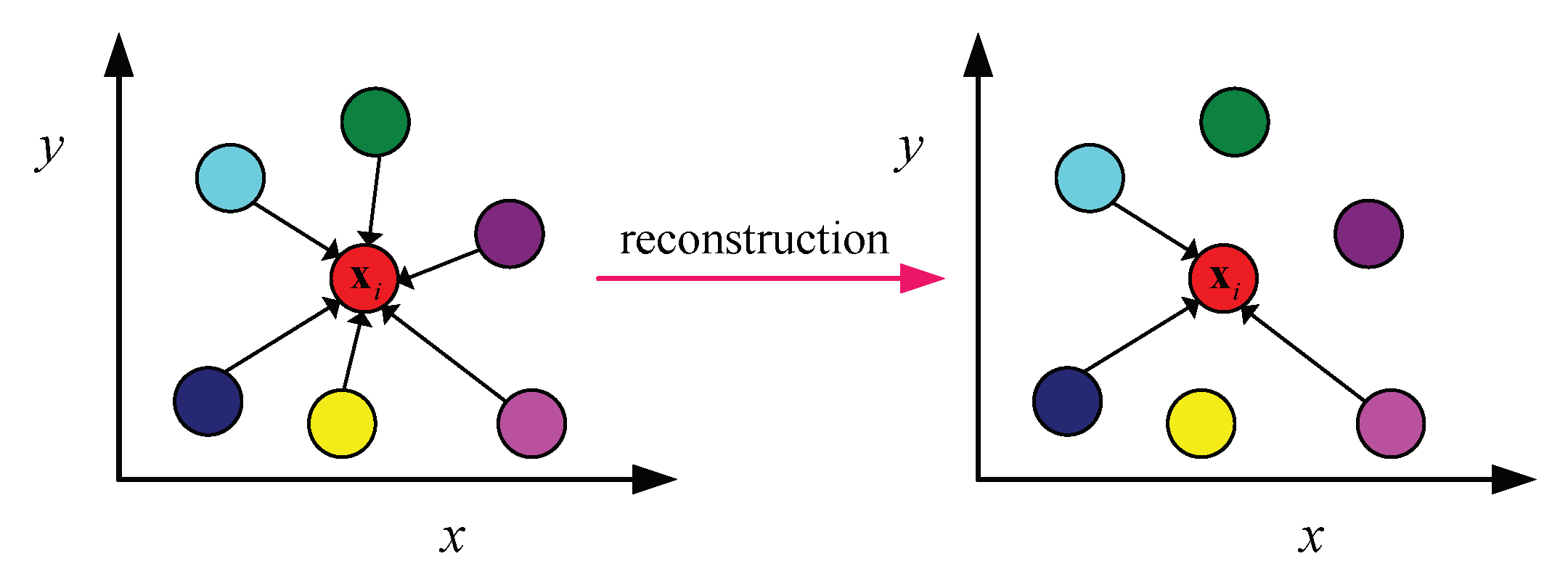
In this paper, to enhance the robustness of the reconstruction error of data points and select the discriminative features, we apply the L2,1-norm loss function and a reconstruction error term. More specifically, in the incomplete data set, instance is only reconstructed by a few important neighbors, rather than being reconstructed by all the instances (as illustrated in Figure 1).
Based on the observed cases in which each instance has a different missing value in an incomplete data set, we cannot apply an optimization algorithm to obtain the weight matrices and . In order to take into account the observed information in an incomplete data set, the indicator matrix is employed. To minimize the reconstruction error and the residual loss term and to preserve the incomplete data manifold structure, we can express the problem as follows:
where ∘ is the Hadamard product, which enables us to formulate the objective function of the proposed unsupervised feature selection for incomplete data (UFS-ID) method.The first term in problem (6) is used to minimize the loss function of and the second term is used to minimize the reconstruction error of data instances. To preserve the incomplete data structure, the third term, for structure embedding, is added into the problem (6), and the fourth term of problem (6) is used to force the matrix to havesparsity and robustness. Since these four terms of the objective function in (6) are related to each other, they can jointly improve the performance of feature selection in an incomplete data set.
Remark 1.
λ is a nonnegative tuning parameter used to control the sparsity of the feature weight coefficient matrix , β is a nonnegative tuning parameter used to balance the structure embedding in the problem (6), and γ is a nonnegative parameter used to control the reconstruction error of data instances. In our experiments, we observed that the results of the proposed approach were sensitive to the regularization parameters γ, β, and λ, so these parameters were all tuned in the grid in our experiments.
3.2.3. Optimization of Objective Function
Solving Equation (6) is challenging, because it introduces two variables, and . We thus solve the problem by means of an alternative optimization strategy, alternatively optimizing the two variables and .
- (1)
- Update by Fixing
Before updating , to derive the optimization of the objective function, we must first make the following observation about the L2,1 norm based on algebraic theory:
where is a diagonal matrix, of which the i-th element is defined as .
Let ; when is fixed, (6) is simplified into (7):
where and indicate a diagonal matrix, of which the i-th element is defined as
and , is the Laplacian matrix. is also a diagonal matrix, of which the i-th element is .
By taking the derivative of problem (7) with respect to and setting it to zero, we have
Hence, we obtain the following solution of :
- (2)
- Update by Fixing
When is fixed, problem (6) becomes
where is a diagonal matrix, of which the i-th element is defined as
and the -th entry of matrix is .
The derivative of (12) with respect to is
Hence, the solution of is
We summarize the detailed UFS-ID optimization approach in Algorithm 1.
| Algorithm 1 Proposed Algorithm for Optimizing (6) |
| Input: Incomplete dataset , regularization parameter , , , and feature selection number k. output: , . (1) Initialize , , R. (2) After setting different missing ratios, calculate the indicator matrix according to (1). (3) Calculate . (4) Fixed , calculated according to (11). (5) Fixed , calculated according to (15). (6) Repeat steps (4) and (5) until convergence. (7) Use the calculated results to select the features. |
3.2.4. Convergence Analysis
To prove the convergence of the proposed algorithm, we need the following lemma [29].
Lemma 1.
For any integers p, q, the following inequality is always true:
The convergence of the Algorithm 1 is summarized in the following theorem.
Theorem 1.
The objective function value in problem (6) monotonically decreases until convergence by updating matrix in Algorithm 1.
Proof.
For convenience, we define
is denoted as the updated , since becomes smaller in each iteration and, in the light of L2,1-norm minimization [29], we have
and
Thus, according to the inequalities above, we achieve
This states that the objective function monotonically decreases by updating in each iteration. □
3.3. Supervised Feature Selection for Incomplete Data
3.3.1. The Basic Supervised Feature Selection Method
The difference between the method described in this sectionand the unsupervised method is that the data set used in this section has a label set , where c is the total number of classes in the data set. Recently, structured sparsity has been used for classification-based feature selection, and structured sparsity has been efficiently applied to the selection of useful features, such as LASSO.
With regards to traditional ridge regression, instead of applying the squared L2-norm regularization, the supervised feature selection methods can be formulated by imposing L2,1-norm regularization:
where is the projection matrix and the Frobenius norm of is .
In this paper, we further focus on some important features that are only correlated to a subset of classes. Since the L2,1 norm cannot handle these cases properly, the supervised feature selection framework can be formulated by adding an L1-norm regularizer:
3.3.2. The Objection Function of Supervised Feature Selection on Incomplete Data
In this section, by virtue of the proposed UFS approach with the reconstruction error and robust loss function, a supervised feature selection approach based on a reconstruction model L2,1 norm and an L1-norm regularizer is imposed to minimize the loss term error and the reconstruction error.
Similarly to the UFS approach, the indicator matrix is imposed to prevent unobserved information from interfering with the feature selection process.We propose a novel supervised feature selection approach for incomplete data set via the following objective function, namely, supervised feature selection for incomplete data (SFS-ID):
where is the reconstruction weight matrix, which can be used to measure the degrees of contribution of the classes in order to reconstruct each instance in an incomplete data set. The first term of problem (24) is used to minimize the reconstruction error between the value of the class and a linear combination of its selected features after projection for an incomplete data set. The second and third items are used to impose the weight matrix to ensure sparseness for the supervised feature selection process.
Note that the last two items of problem (24) are included to ensure that the weight matrix has both robustness and sparsity, because the robustness loss is smoothly interpolated between L2,1 and the Frobenius norm, which can respectively prevent excessive overfitting and obtain sparsity for effective feature selection. Since the four components of the objective function in (24) are interrelated, they can jointly improve the performance of feature selection in incomplete data sets.
3.3.3. Optimization of Objective Function
In this section, we present the optimization of the above objective function. Although the above objective function is convex, solving problem (24) is still difficult, because the two regularization terms are non-smooth and the two variables and need to be optimized simultaneously. We propose an efficient algorithm to solve this problem by alternatively optimizing variables and , respectively.
(1) Update by Fixing
Let ; thus, the problem (24) becomes
Taking the derivative of problem (25) with respect to by setting (26) to zero, we have
where () is a diagonal matrix, of which the k-th element is denoted by , where is a diagonal matrix .
Hence, we can obtain the solution of :
(2) Update by Fixing
When is fixed, problem (24) becomes
Furthermore, according to the Frobenius norm framework, (27) can be rewritten as
By taking the derivative of problem (28) with respect to and setting it to zero, we have
Hence, we can obtain the solution of :
Based on the above derivation, the whole SFS-ID procedure for optimizing the problem (24) is summarized in Algorithm 2.
| Algorithm 2 Proposed Algorithm for Optimizing (24) |
| Input: Incomplete dataset , , regularization parameter , . output: . (1) Initialize , , , . (2) After setting different missing ratios, calculate the indicator matrix . (3) Calculate . (4) Fixed , the optimal is formed by (27). (5) Fixed , Calculate the diagonal matrix according to (31). (6) Repeat steps (3)–(5) until convergence. (7) Use the calculated results to select the features. |
3.3.4. Convergence Analysis
The convergence of the Algorithm 2 is summarized in the following theorem.
Theorem 2.
The objective function value in problem (24) monotonically decreases until convergence by updating matrix in Algorithm 2.
Proof.
For convenience, we define
In addition, the updated is defined by ; according to Algorithm 2, we have
Since becomes smaller in each iteration, we have
where and is the function of . According to this analysis, we obtain
According to Lemma 1, for any vector w and , we obtain
Furthermore, by combining the two inequalities above, we have
which shows that the objective function decreases monotonically by updating in each iteration. □
4. Experiment and Result Analysis
In this section, we describe the exhaustive numerical experiments conducted on incomplete data sets to validate the effectiveness of the proposed UFS-ID and SFS-ID methods.
4.1. Unsupervised Feature Selection
4.1.1. Evaluation Metrics
We compared the clustering performance of our UFS-ID method with that of competing approaches on five incomplete data sets. Similarly to previous works, we evaluated the performance of UFS methods using two extensively employed evaluation metrics: clustering accuracy (ACC) and normalized mutual information (NMI). ACC denotes the percentage of samples that are correctly classified, and it can be computed as follows:
where n is the number of instances and denotes the number of correctly clustered instances. Hence, a larger ACC indicates better performance.
NMI expresses the correlation between the predicted labels and the real labels, that is,
where is the number of instances in the cluster , is the number of instances in the cluster , and denotes the number of instances in the set.
All experiments were carried out on a PC installed with Matlab2019a, Intel Core i7-8750H CPU, and 16-GB RAM. We adopted the tenfold cross-validation scheme, and the number of clusters in the k-means clustering was set to the absolute number of classes in the data set.
The parameters used in the comparison schemes were consistent with the corresponding literature and the regularization parameters , , and were all tuned in the grid in our experiments.
Moreover, in our experiments, paired-sample t-tests (at the 95% significance level) between our UFS-ID method and competing UFS methods were adopted in terms of ACC and NMI. Specifically, the symbols “*” and “**” denote that our UFS-ID method had statistically significant differences with and , respectively, in the paired-sample t-tests at the 95% significance level compared with the other competing UFS methods.
4.1.2. Dataset
Five real data sets were used in our experiments https://archive.ics.uci.edu/ml/datasets.php (accessed on 1 January 2021), including CNAE, cifar, connect-4, vehicle, and USPSt. Detailed information on the data sets is provided in Table 2.
In this work, we defined the incomplete instance ratio as the percentage of incomplete instances out of the total number of samples. To determine the incomplete instance ratio, we randomly marked a portion of the observed information as unobserved information, setting the incomplete instance ratio within a range of 0% to 90%, increasing at an interval of 10%.
4.1.3. Comparison Schemes
For convenience, the incomplete data set was divided into two parts, i.e., the incomplete set (IS), containing all incomplete instances, and the observed set (OS), containing all observed instances. To verify the effectiveness of the proposed UFS-ID method, we compared it with the following competing UFS methods for incomplete data sets:
- For the baseline, we used the k-means clustering algorithm with all features of OS.
- Lapscore [25] is a filter method that evaluates the importance of each feature based on its Laplacian score. It selects features of the OS.
- GSR [28] is a general framework which unifies a sparse embedding model and feature selection together. It selects features of the OS.
- RFS [29] is another typical embedded model of feature selection which has proven its effectiveness in reducing the influence of outliers. It selects features of the OS.
- GSR_mean is an imputation feature selection framework, which uses the mean-value imputation method [15] on the IS, and selects feature from the union of the IS and OS using GSR.
- GSR_KNN is imputation feature selection framework, which uses KNN imputation method [12] on the IS, and selects features from the union of the IS and OS using GSR.
- GSR_missForest [18] is an iterative imputation framework based on random forest on the IS, which selects features from the union of the IS and OS using GSR.
- GSR_DGM [20] is a probabilistic framework based on deep generative models for missing value imputation on the IS, which selects features from the union of the IS and OS using GSR.
- GSR_MIWAE [21] is an importance-weighted autoencoder framework, which maximizes a potentially tight lower bound of the log-likelihood on the IS, and selects features from the union of the IS and OS using GSR.
- HQ-UFS [23] is a framework for incomplete data sets, in which the half-quadratic minimization technique is used to make the weight of outliers more negligible or even zero and reducing the influence of outliers. It selects features directly from the incomplete data set.
4.1.4. Experimental Results
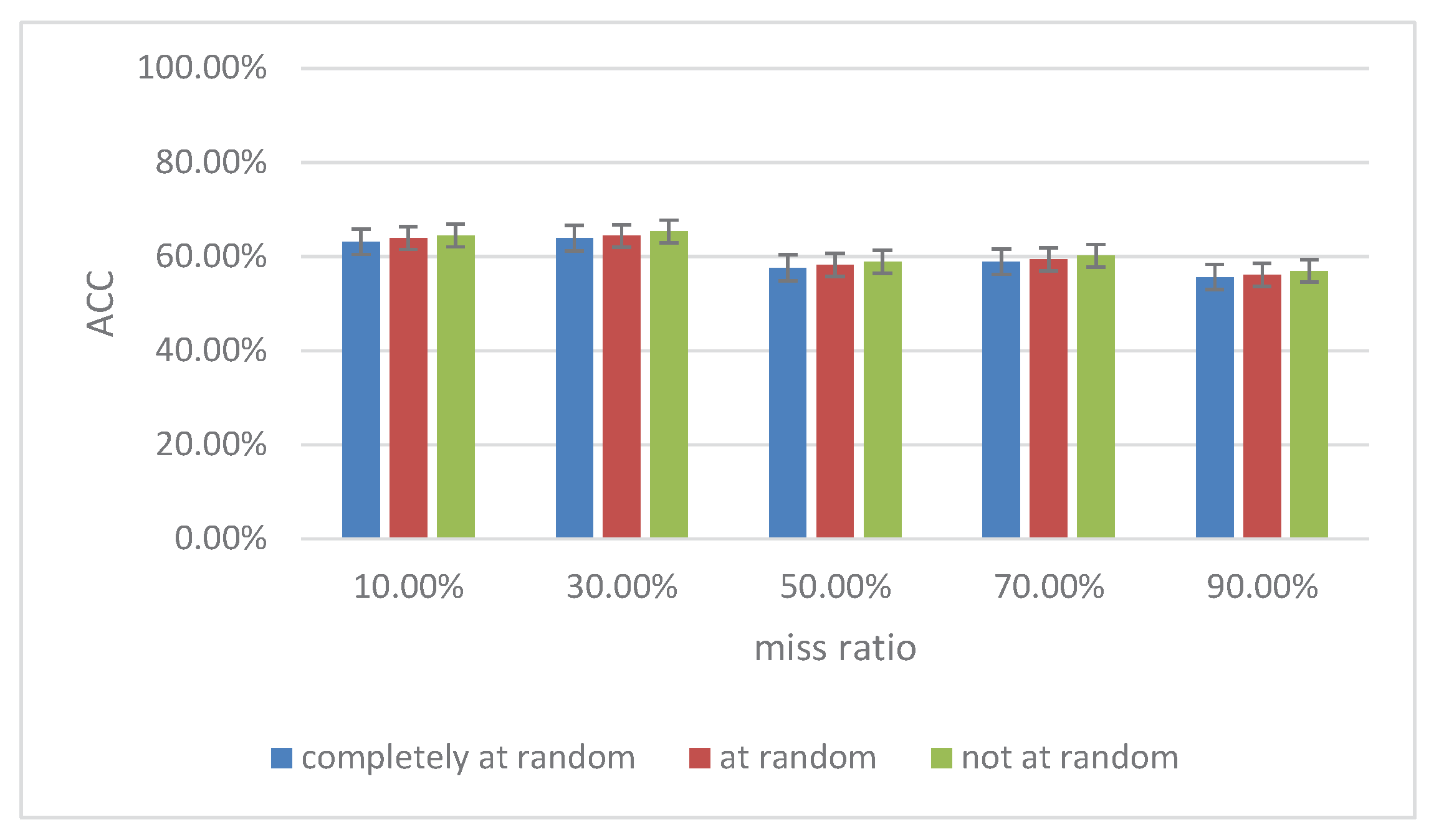
Firstly, we compared our UFS-ID method with three popular types of missing data values, i.e., completely at random, at random (conditioned on values in another randomly chosen column, being in a random interval) or not at random (conditioned on values to be missed). In these experiments, we used the CANE data set to evaluate the effectiveness of different types of data values missed. In Figure 2 the relative ACC is shown in a given condition. From the figure, we can obviously see that our method worked well in respect to the three popular types of data values missed, even in the difficult missing-not-at-random condition. Furthermore, our UFS-ID method with the non-random-type dataachieved better performance compared to other two types. For convenience, completely random-type data were adopted for use in the subsequent experiments.
Secondly, we selected features with different incomplete instances ratios (i.e., 0, 10%, 30%, 50%, 70%, 90%) to perform clustering tasks, and the clustering results were obtained, as shown in Table 3. The best results are denoted in bold in the table.
Based on the results shown in Table 3, we concluded that our UFS-ID approach achieved the best clustering performance compared to other competing UFS methods on incomplete data. In addition, the clustering results of our UFS-ID approach were statistically significantly better than those of all comparison methods in term of ACC and NMI. In particular, it can easily be verified from the table that the performance of the UFS-ID approach represented a great improvement in the large and small incomplete data set. Through further analysis of the experiment results, we can draw the following conclusions.
- (1)
- As the incomplete instance ratio increased, the performance of all schemes dropped sharply. For instance, on the cifar data set, the ACC of all schemes dropped by 1.31% on average at a ratio of 0.1, compared with a ratio of 0.9. In addition, on the vehicle data set, the ACC of all schemes dropped by 5.41% on average at a ratio of 0.1, compared with a ratio of 0.9. It also can be verified that most of the schemes achieved the best performance with small ratios, showing that the number of complete instances played an important role in those feature selection schemes.
- (2)
- The performance of our UFS-ID approach was similar to that of imputation and HQ-UFS approaches. It achieves better performance compared with other traditional feature selection approaches on the OSs of incomplete data sets. For example, on the USPSt data set, the UFS-ID approach achieved around 3.0% and 5.5% improvements at the ratios of 0.1 and 0.9, compared with RFS. This indicates that the more information is employed for the imputation, the more similar is the performance of HQ-UFS and UFS-ID.
- (3)
- The performance of GSR_knn, GSR_mean, GSR_missForest, GSR_DGM, GSR_MIWAE, and HQ-UFS was worse than that of our UFS-ID method. The reason for this is that UFS-ID utilizes neighbor data reconstruction information to improve the incomplete data structure for the selection of discriminative features, whereas other approaches do not add the information derived from neighbor data.
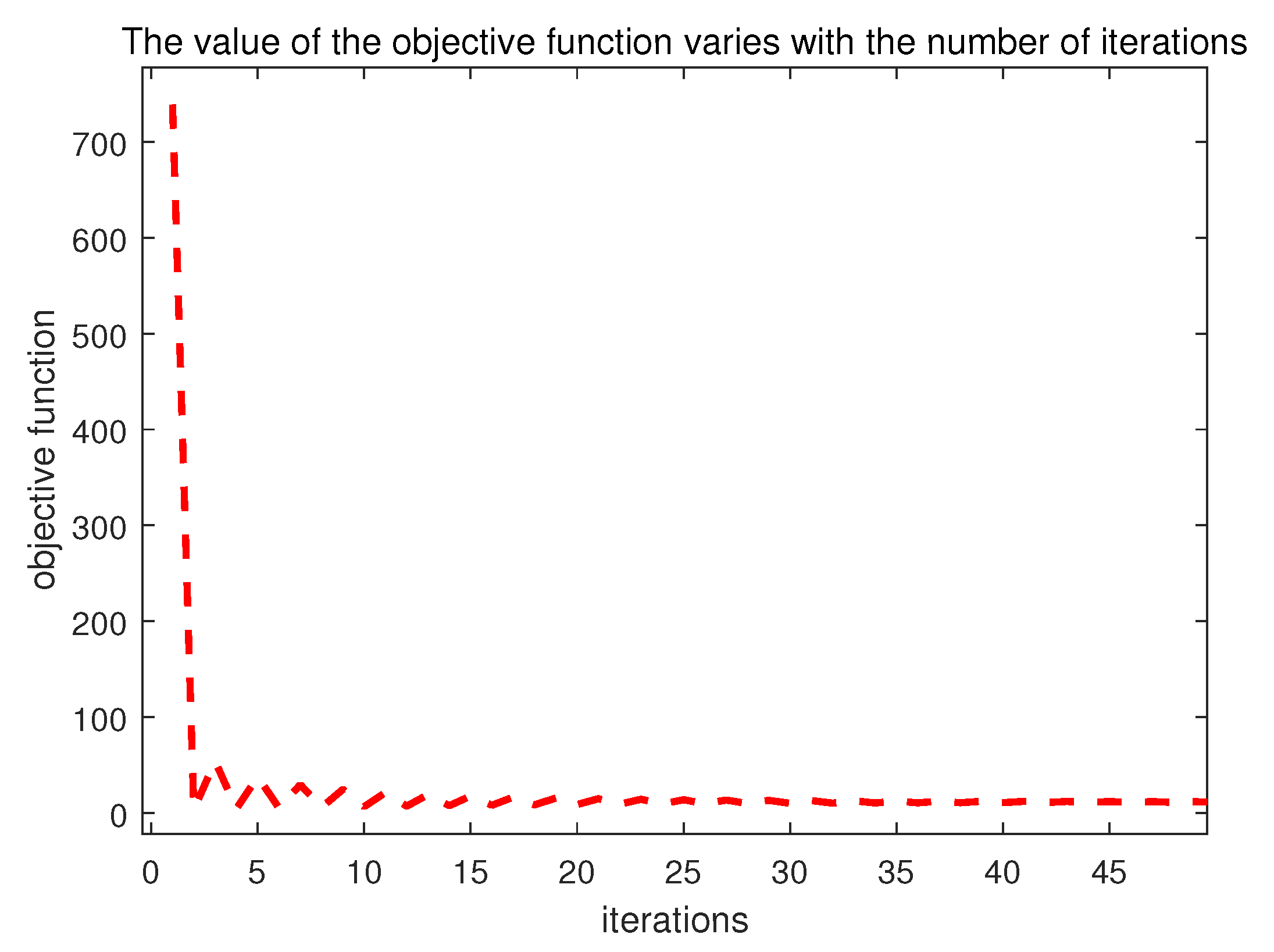
Finally, in Section 3.2, the convergence of the proposed algorithm in solving the objective function, namely, (6), is theoretically proven. Figure 3 shows the variation of the objective function value on the Iris data set with the number of iterations; it displays the convergence curve of the proposed UFS-ID approach, which showed a fast convergence.
4.2. Supervised Feature Selection
4.2.1. Dataset
To evaluate the effectiveness of Algorithm 2, we conducted experiments on synthetic data sets and real data sets, respectively.
The synthetic data set contained 500 instances and 100-dimensional features. Five-hundred instances in 100-dimensional space were generated, in which two features defined an XOR function, whereas the remaining 98 features were irrelevant, sampled independently from a zero-mean and one-standard-deviation normal distribution.
We also present the results obtained on six real data sets, called DLBCL, Mnist, Splice, Wpbc, USPS, and Arcene. Since the Splice and Wpbc datasets had fewer features, we artificially added 2000 irrelevant features to them, and the feature values of the irrelevant features were all obtained by sampling from the normal distribution . The detailed information on the data sets is shown in Table 4.
4.2.2. Comparison Methods and Experimental Settings
To verify the effectiveness of the proposed SFS-ID method with the synthetic data sets, we compared it with four competing SFS methods designed for use on incomplete data sets, including:
- The SID method [13], a framework in which the objective function takes into account the uncertainty of instances due to the missing values and which solves the revised optimization problem using an EM algorithm;
- Mean, an imputation feature selection framework, which uses the mean-value imputation method [15] on the IS, and which selects features from the union of the IS and OS using RFS;
- EM, an imputation feature selection framework, which uses the EM imputation method [16] on the IS and which selects feature from the union of the IS and OS using RFS;
- missForest [18], an iterative imputation framework based on a random forest on the IS, which selects features from the union of the IS and OS using RFS;
- DGM [20], a probabilistic framework based on the use of deep generative models for missing value imputation on the IS, and which selects feature from the union of the IS and OS using RFS; and
- MIWAE [21], an importance-weighted autoencoder framework, which maximizes a potentially tight lower bound of the log-likelihood on the IS and selects features from the union of the IS and OS using RFS.
Unlike the synthetic data, in the experiments on real data sets, the optimal features are unknown as there might be some uncorrelated and weakly correlated features in incomplete data sets. We trained an SVM classifier on the features selected using different methods, and the classification error value was reported. For the SVM classifier, we adopted a Gaussian kernel and its width was set as the median distance between points in the instance. Ten cross-validations on data sets were are conducted in this experiment.
We compared the results of our method with those of the following competing SFS methods on incomplete data sets: KNN + RFS, KNN + Simba, KNN + Relief, mean + RFS, mean + Simba, mean + Relief, EM + RFS, EM + Simba, EM + Relief, missForest + RFS, missForest + Simba, missForest + Relief, DGM + RFS, DGM + Simba, DGM + Relief, MIWAE + RFS, MIWAE + Simba, MIWAE + Relief, and SID.
The parameters in the comparison schemes were consistent with the corresponding literature and the regularization parameters and in our proposed method were all tuned in the grid .
4.2.3. Experimental Results
(1) Experiments on Synthetic Data Sets
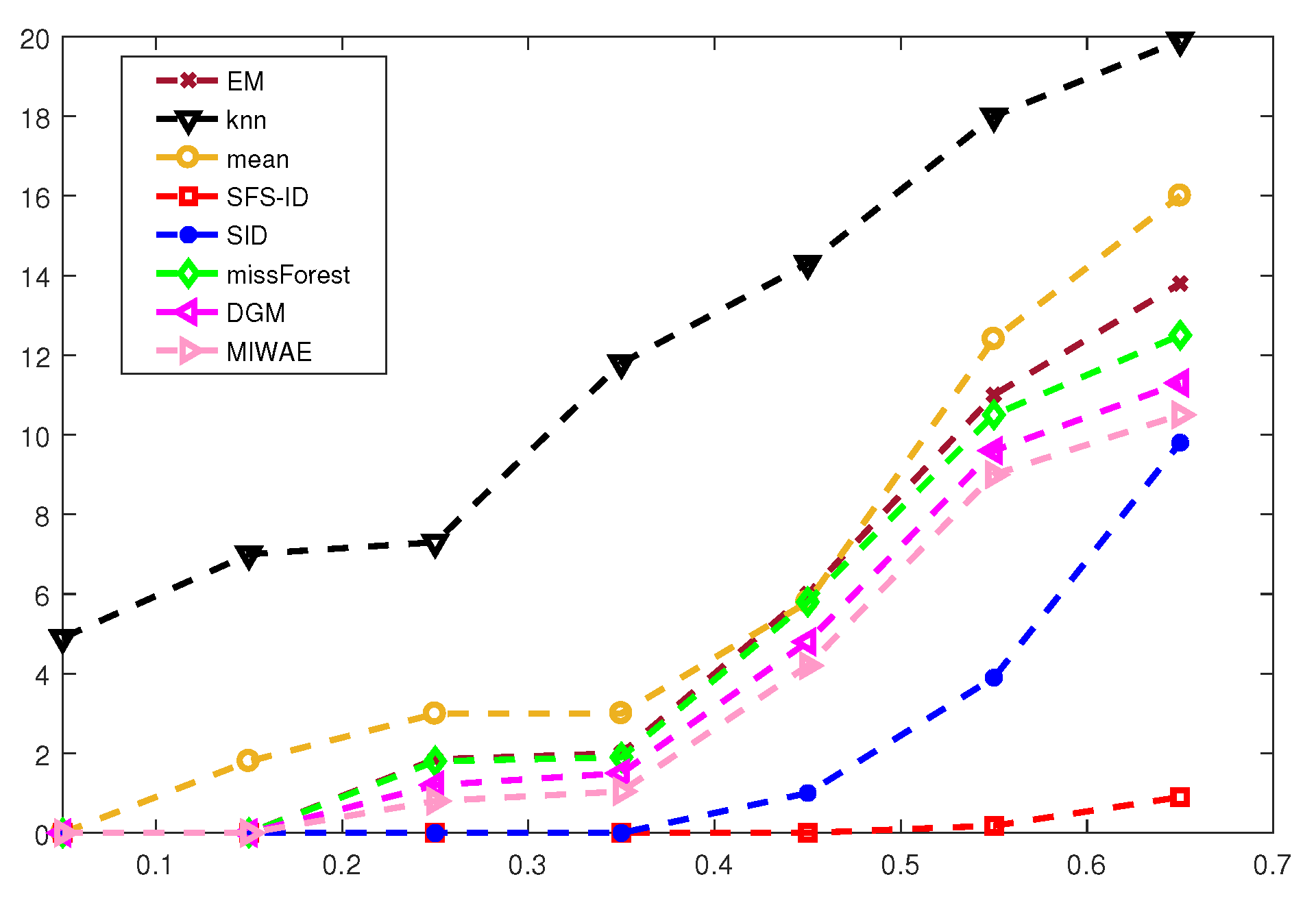
We used the number of irrelevant features, selected by means of SFS-ID and other state-of-the-art approaches, as a performance index in the experiments on synthetic data. The results are shown in Figure 4.
Based on the results shown in Figure 4, we concluded that the proposed SFS-ID approach clearly outperformed other state-of-the-art SFS approaches. In particular, with the increase in the missing ratio, the number of irrelevant features of all methods increased, but SFS-ID was still able to select the only two relevant features in the presence of 55% of missing values. Hence, if the missing ratio is excessively large, our SFS-ID can choose relevant features and thus improve the classification performance.
(2) Experiments on Real Data Sets
We used the features selected by the feature to build an SVM classification model. As an evaluation metric, classification accuracy (Acc) was used to measure the performance of different approaches.
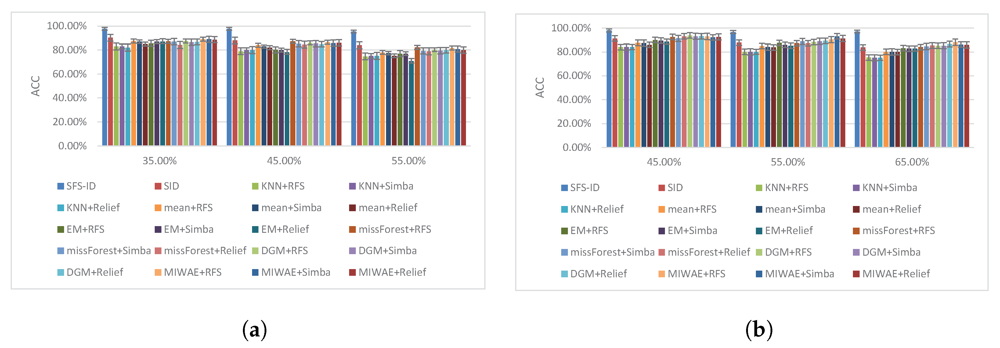
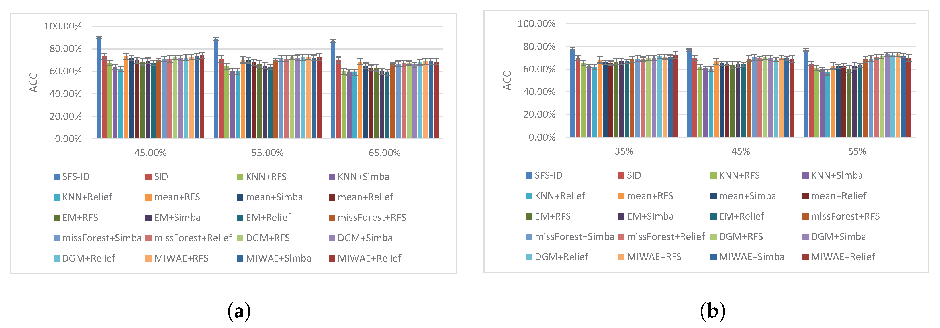
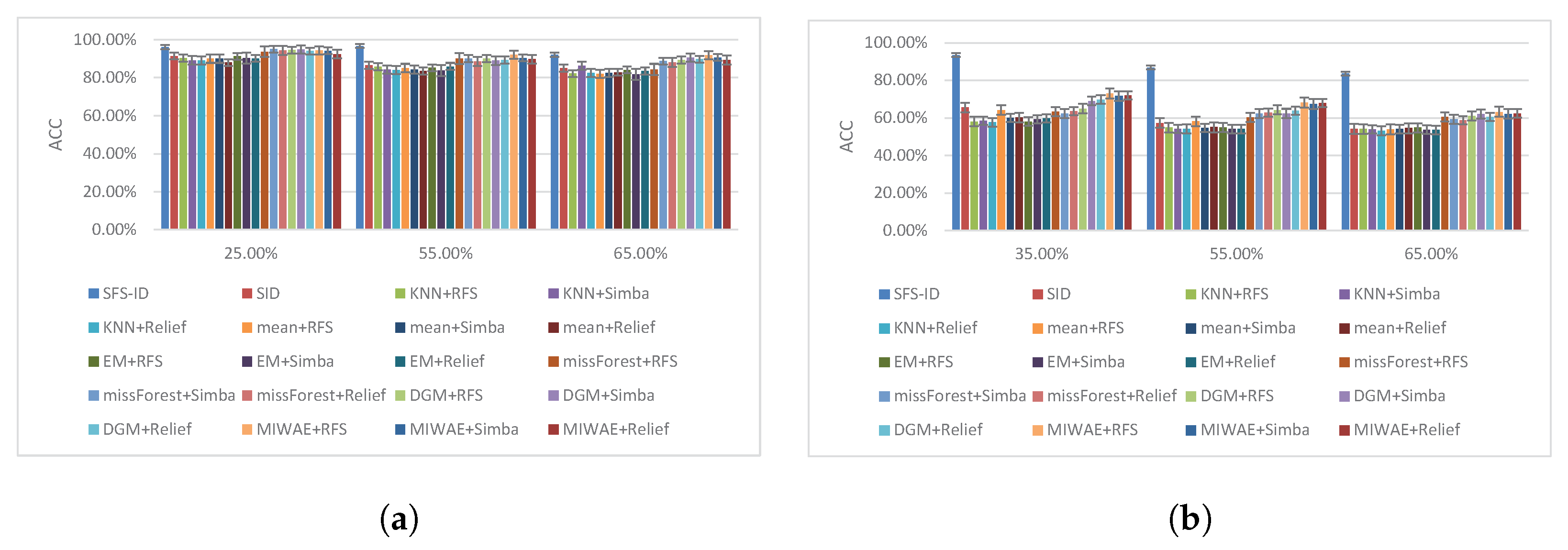
We selected the features with different missing instance ratios to perform classification tasks, and the classification results are shown in Figure 5, Figure 6 and Figure 7.
Based on the results shown in Figure 5, Figure 6 and Figure 7, we concluded that our SFS-ID approach achieved the best classification performance compared to other competing SFS methods on incomplete data. In addition, the classification results of our SFS-ID approach were statistically significantly better than those of all comparison methods in terms of ACC. In particular, it can easily be verified from the figure that the performance of the SFS-ID approach showed a great improvement in the large and small incomplete data sets. Through further analysis of the other experimental results, we drew the following conclusions.
First, as the incomplete instances ratio increased, the performance of all schemes sharply dropped. For instance, on the Mnist data set, the ACC of all schemes dropped by 6.9% on average at a ratio of 0.45, compared with a ratio of 0.65. In addition, on the USPS data set, the ACC of all schemes dropped on average by 5.78% at a ratio of 0.25, compared with a ratio of 0.65. It also can be verified that most of schemes achieved the best performance with a small ratio, which shows that the number of complete instances played an important role in those feature selection schemes.
Second, compared with those of other approaches, the ACC of our SFS-ID method decreased more slowly with the missing ratio. For example, on the Mnist data set, the performance of SFS-ID approach decreased by around 1.0% at the missing ratio of 0.45, compared to the ratio of 0.65, whereas the performance of SID, KNN+RFS, and MIWAE+RFS decreased by 7.49%, 8.7%, and 4.76%, respectively. The reason for this is that SFS-ID utilized neighbor data reconstruction information to improve the incomplete data structure for the selection of discriminative features, whereas other approaches do not incorporate information from neighbor data.
5. Conclusions
In this paper, we have proposed novel unsupervised and supervised feature selection approaches (UFS-ID and SFS-ID), which integrate the reconstruction error and L2,1-norm minimization for feature selection. By using prior knowledge of incomplete data, not only can the data reconstruction be made more representative, but the L2,1-norm minimization-sparse modelcan select robustly important features as well. Alternative iterative algorithms to effectively optimize the proposed objective functions were designed and the convergence of the proposed algorithms was proven theoretically. Eventually, we will performextensive experiments on both real and synthetic incomplete data sets to verify the effectiveness and superiority of the proposed approaches.
Author Contributions
Conceptualization, J.C.; Data curation, J.C.; Formal analysis, J.C. and L.F.; Funding acquisition, X.X.; Investigation, J.C.; Project administration, X.X.; Resources, X.X. and X.W.; Software, X.X. and L.F.; Visualization, J.C.; Writing—original draft, J.C.; Writing—review & editing, X.X. and X.W. All authors have read and agreed to the published version of the manuscript.
Funding
This work has been supported by the National Natural Science Foundation of China (No.61802425, 62171466 and 62001515).
Institutional Review Board Statement
Not applicable.
Informed Consent Statement
Not applicable.
Data Availability Statement
Not applicable.
Conflicts of Interest
The authors declare no conflict of interest.
References
- Cover, T.M. Elements of Information Theory; John Wiley & Sons: Hoboken, NJ, USA, 1999. [Google Scholar]
- Hart, P.E.; Stork, D.G.; Duda, R.O. Pattern Classification; John Wiley & Sons: Hoboken, NJ, USA, 2000. [Google Scholar]
- Lee Rodgers, J.; Nicewander, W.A. Thirteen ways to look at the correlation coefficient. Am. Stat. 1988, 42, 59–66. [Google Scholar] [CrossRef]
- Solorio-Fernández, S.; Carrasco-Ochoa, J.A.; Martínez-Trinidad, J.F. A review of unsupervised feature selection methods. Artif. Intell. Rev. 2020, 53, 907–948. [Google Scholar] [CrossRef]
- Feng, Y.; Xiao, J.; Zhuang, Y.; Liu, X. Adaptive unsupervised multi-view feature selection for visual concept recognition. In Proceedings of the Asian Conference on Computer Vision, Daejeon, Korea, 5–9 November 2012; Springer: Berlin/Heidelberg, Germany, 2012; pp. 343–357. [Google Scholar]
- Krzanowski, W.J. Selection of variables to preserve multivariate data structure, using principal components. J. R. Stat. Soc. Ser. C 1987, 36, 22–33. [Google Scholar] [CrossRef]
- Sa, W.; Ke-yong, W.; Lian, Z. Feature Selection via Analysis of Relevance and Redundancy. J. Beijing Inst. Technol. 2008, 17, 300–304. [Google Scholar]
- Zhu, P.; Zuo, W.; Zhang, L.; Hu, Q.; Shiu, S.C. Unsupervised feature selection by regularized self-representation. Pattern Recognit. 2015, 48, 438–446. [Google Scholar] [CrossRef]
- Zhu, X.; Yang, J.; Zhang, C.; Zhang, S. Efficient utilization of missing data in cost-sensitive learning. IEEE Trans. Knowl. Data Eng. 2019, 33, 2425–2436. [Google Scholar] [CrossRef]
- Zhou, Y.; Tian, L.; Zhu, C.; Jin, X.; Sun, Y. Video coding optimization for virtual reality 360-degree source. IEEE J. Sel. Top. Signal Process. 2019, 14, 118–129. [Google Scholar] [CrossRef]
- Van Hulse, J.; Khoshgoftaar, T.M. Incomplete-case nearest neighbor imputation in software measurement data. Inf. Sci. 2014, 259, 596–610. [Google Scholar] [CrossRef]
- Zhang, S.; Li, X.; Zong, M.; Zhu, X.; Wang, R. Efficient kNN classification with different numbers of nearest neighbors. IEEE Trans. Neural Netw. Learn. Syst. 2017, 29, 1774–1785. [Google Scholar] [CrossRef]
- Lou, Q.; Obradovic, Z. Margin-based feature selection in incomplete data. In Proceedings of the AAAI Conference on Artificial Intelligence, Toronto, ON, Canada, 22–26 July 2012; Volume 26. [Google Scholar]
- Cismondi, F.; Fialho, A.S.; Vieira, S.M.; Reti, S.R.; Sousa, J.M.; Finkelstein, S.N. Missing data in medical databases: Impute, delete or classify? Artif. Intell. Med. 2013, 58, 63–72. [Google Scholar] [CrossRef]
- Garcia, C.; Leite, D.; Škrjanc, I. Incremental missing-data imputation for evolving fuzzy granular prediction. IEEE Trans. Fuzzy Syst. 2019, 28, 2348–2362. [Google Scholar] [CrossRef]
- Simone, R. An accelerated EM algorithm for mixture models with uncertainty for rating data. Comput. Stat. 2021, 36, 691–714. [Google Scholar] [CrossRef]
- Pan, R.; Yang, T.; Cao, J.; Lu, K.; Zhang, Z. Missing data imputation by K nearest neighbours based on grey relational structure and mutual information. Appl. Intell. 2015, 43, 614–632. [Google Scholar] [CrossRef]
- Stekhoven, D.J.; Bühlmann, P. MissForest-non-parametric missing value imputation for mixed-type data. Bioinformatics 2012, 28, 112–118. [Google Scholar] [CrossRef]
- Gondara, L.; Wang, K. Multiple imputation using deep denoising autoencoders. arXiv 2017, arXiv:1705.02737. [Google Scholar]
- Zhang, H.; Xie, P.; Xing, E. Missing value imputation based on deep generative models. arXiv 2018, arXiv:1808.01684. [Google Scholar]
- Mattei, P.A.; Frellsen, J. MIWAE: Deep generative modelling and imputation of incomplete data sets. In Proceedings of the International Conference on Machine Learning, Long Beach, CA, USA, 9–15 June 2019; pp. 4413–4423. [Google Scholar]
- Le Morvan, M.; Josse, J.; Scornet, E.; Varoquaux, G. What is a good imputation to predict with missing values? Adv. Neural Inf. Process. Syst. 2021, 34, 11530–11540. [Google Scholar]
- Shen, H.T.; Zhu, Y.; Zheng, W.; Zhu, X. Half-quadratic minimization for unsupervised feature selection on incomplete data. IEEE Trans. Neural Netw. Learn. Syst. 2020, 32, 3122–3135. [Google Scholar] [CrossRef]
- Lazar, C.; Taminau, J.; Meganck, S.; Steenhoff, D.; Coletta, A.; Molter, C.; de Schaetzen, V.; Duque, R.; Bersini, H.; Nowe, A. A survey on filter techniques for feature selection in gene expression microarray analysis. IEEE/ACM Trans. Comput. Biol. Bioinform. 2012, 9, 1106–1119. [Google Scholar] [CrossRef]
- He, X.; Cai, D.; Niyogi, P. Laplacian score for feature selection. Adv. Neural Inf. Process. Syst. 2005, 18, 507–514. [Google Scholar]
- Kabir, M.M.; Islam, M.M.; Murase, K. A new wrapper feature selection approach using neural network. Neurocomputing 2010, 73, 3273–3283. [Google Scholar] [CrossRef]
- Peng, C.; Kang, Z.; Yang, M.; Cheng, Q. Feature selection embedded subspace clustering. IEEE Signal Process. Lett. 2016, 23, 1018–1022. [Google Scholar] [CrossRef]
- Peng, H.; Fan, Y. A general framework for sparsity regularized feature selection via iteratively reweighted least square minimization. In Proceedings of the AAAI Conference on Artificial Intelligence, San Francisco, CA, USA, 4–9 February 2017; Volume 31. [Google Scholar]
- Nie, F.; Huang, H.; Cai, X.; Ding, C. Efficient and robust feature selection via joint ℓ2,1-norms minimization. Adv. Neural Inf. Process. Syst. 2010, 23, 1813–1821. [Google Scholar]
- Shu, W.; Shen, H. Multi-criteria feature selection on cost-sensitive data with missing values. Pattern Recognit. 2016, 51, 268–280. [Google Scholar] [CrossRef]
- Fan, L.; Wu, X.; Tong, W.; Zeng, W. L2,1-norm minimization for Unsupervised Feature Selection from Incomplete Data. In Proceedings of the 2021 7th International Conference on Computer and Communications (ICCC), Chengdu, China, 10–13 December 2021; pp. 1491–1495. [Google Scholar]
- Gilad-Bachrach, R.; Navot, A.; Tishby, N. Margin based feature selection-theory and algorithms. In Proceedings of the Twenty-First International Conference on Machine Learning, Banff, AB, Canada, 4–8 July 2004; p. 43. [Google Scholar]
- Kira, K.; Rendell, L.A. A practical approach to feature selection. In Machine Learning Proceedings 1992; Elsevier: Amsterdam, The Netherlands, 1992; pp. 249–256. [Google Scholar]
- Lou, Q.; Obradovic, Z. Modeling multivariate spatio-temporal remote sensing data with large gaps. In Proceedings of the Twenty-Second International Joint Conference on Artificial Intelligence, Barcelona, Spain, 16–22 July 2011. [Google Scholar]
- Grangier, D.; Melvin, I. Feature set embedding for incomplete data. Adv. Neural Inf. Process. Syst. 2010, 23, 793–801. [Google Scholar]
- Śmieja, M.; Struski, Ł.; Tabor, J.; Marzec, M. Generalized RBF kernel for incomplete data. Knowl. Based Syst. 2019, 173, 150–162. [Google Scholar] [CrossRef]
- Przewiezlikowski, M.; Smieja, M.; Struski, L.; Tabor, J. MisConv: Convolutional Neural Networks for Missing Data. In Proceedings of the WACV, Waikoloa, HI, USA, 4–8 January 2022; pp. 2917–2926. [Google Scholar]
- Zhang, R.; Li, X. Unsupervised feature selection via data reconstruction and side information. IEEE Trans. Image Process. 2020, 29, 8097–8106. [Google Scholar] [CrossRef]
Figure 1.
Instance is only reconstructed by a few important neighbors in an incomplete data set, rather than being reconstructed by all the instances.
Figure 1.
Instance is only reconstructed by a few important neighbors in an incomplete data set, rather than being reconstructed by all the instances.

Figure 2.
Comparison of ACC performance across the CANE data set with three varying types of missing data values.
Figure 2.
Comparison of ACC performance across the CANE data set with three varying types of missing data values.

Figure 3.
Convergence curve of the proposed UFS-ID approach.

Figure 4.
The number of irrelevant features selected, together with two relevant features.

Figure 5.
Accuracy under different missing ratios for DLBCL and Mnist datasets. (a) DLBCL. (b) Mnist.
Figure 5.
Accuracy under different missing ratios for DLBCL and Mnist datasets. (a) DLBCL. (b) Mnist.

Figure 6.
Accuracy under different missing ratios for Splice and Wpbc datasets. (a) Splice. (b) Wpbc.
Figure 6.
Accuracy under different missing ratios for Splice and Wpbc datasets. (a) Splice. (b) Wpbc.

Figure 7.
Accuracy under different missing ratios for USPS and Arcene datasets. (a) USPS. (b) Arcene.
Figure 7.
Accuracy under different missing ratios for USPS and Arcene datasets. (a) USPS. (b) Arcene.


Table 1.
The notations used in this article.
| Notation | Definition |
|---|---|
| Incomplete data set of n instances and d features | |
| The label set c is the total number of classes | |
| The index matrix indicating whether the information in is complete or not | |
| The feature weight coefficient matrix | |
| The reconstruction weight matrix | |
| Frobenius norm of a matrix | |
| L2,1 norm of a matrix | |
| norm of a function | |
| ∘ | Hadamard product |
Table 2.
Summarization of used data sets.
| Dataset | Instance | Feature | Class |
|---|---|---|---|
| CANE | 1080 | 856 | 9 |
| cifar | 60,000 | 3072 | 10 |
| connect-4 | 67,557 | 126 | 3 |
| vehicle | 78,823 | 126 | 3 |
| USPSt | 2007 | 256 | 10 |
Table 3.
ACC and NMI results for different data sets obtained by all approaches at different instance miss rates. The bold numbers denote the best results for the entire row for the same evaluation metric. Specifically, the symbols “*” and “**” indicate that our UFS-ID method had significantly different outcomes with and on the paired-sample t-test at the 95% significance level, compared with other competing methods.
| Dataset | Ratio | Baseline | LapScore | GSR | RFS | GSR_mean | GSR_knn | GSR_missForest | GSR_DGM | GSR_MIWAE | HQ-UFS | UFS-ID | |||||||||||
|---|---|---|---|---|---|---|---|---|---|---|---|---|---|---|---|---|---|---|---|---|---|---|---|
| ACC | NMI | ACC | NMI | ACC | NMI | ACC | NMI | ACC | NMI | ACC | NMI | ACC | NMI | ACC | NMI | ACC | NMI | ACC | NMI | ACC | NMI | ||
| CNAE | 0 | 48.1 ** ±2.5 | 41.5 ** ±2.5 | 49.9 ** ±2.5 | 41.9 ** ±2.2 | 48.7 ** ±3.0 | 42.1 ** ±2.4 | 54.6 ** ±2.1 | 46.6 ** ±1.7 | 46.4 ** ±2.6 | 40.5 ** ±2.2 | 49.3 ** ±2.5 | 41.7 ** ±2.2 | 51.2 ** ±2.0 | 43.5 ** ±1.9 | 52.6 ** ±2.2 | 44.1 ** ±1.7 | 54.7 ** ±3.0 | 48.7 ** ±3.2 | 55.7 ** ±3.1 | 48.9 ** ±2.9 | 58.8 ±2.9 | 54.9 ±3.0 |
| 0.1 | 46.4 ** ±3.0 | 37.7 ** ±2.3 | 49.1 ** ±3.0 | 40.6 ** ±2.9 | 50.3 ** ±2.2 | 43.3 ** ±2.1 | 55.7 ** ±2.0 | 47.4 ** ±2.8 | 49.4 ** ±1.5 | 41.4 ** ±2.2 | 50.7 ** ±2.1 | 40.9 ** ±2.1 | 57.2 ** ±2.5 | 47.2 ** ±1.8 | 57.5 ** ±1.6 | 47.1 ** ±1.9 | 58.7 ** ±2.4 | 48.2 ** ±2.0 | 58.1 ** ±1.9 | 48.3 ** ±2.6 | 63.1 ±2.3 | 55.8 ±2.3 | |
| 0.3 | 45.4 ** ±3.0 | 37.2 ** ±2.2 | 45.9 ** ±1.9 | 39.9 ** ±1.9 | 52.2 ** ±2.0 | 45.4 ** ±2.1 | 60.1 ** ±3.2 | 52.9 ** ±2.8 | 48.8 ** ±3.6 | 43.0 ** ±2.8 | 53.1 ** ±2.8 | 44.3 ** ±1.5 | 58.2 ** ±3.1 | 51.4 ** ±2.8 | 59.4 ** ±2.3 | 52.0 ** ±2.9 | 61.0 ** ±2.2 | 53.2 ** ±2.5 | 61.2 ** ±3.5 | 53.6 ** ±2.6 | 63.9 ±2.6 | 58.8 ±3.3 | |
| 0.5 | 37.4 ** ±1.6 | 30.8 ** ±1.7 | 52.1 ** ±3.6 | 44.2 ** ±3.7 | 49.1 ** ±3.8 | 42.1 ** ±3.5 | 55.4 ** ±3.3 | 47.5 ** ±2.5 | 42.6 ** ±3.8 | 35.6 ** ±0.3 | 45.3 ** ±3.7 | 37.6 ** ±3.1 | 55.2 ** ±3.2 | 46.2 ** ±2.8 | 55.4 ** ±3.3 | 47.0 ** ±2.3 | 56.0 ** ±3.1 | 47.2 ** ±3.5 | 56.8 ** ±3.5 | 48.0 ** ±3.3 | 57.6 ±3.1 | 51.4 ±2.9 | |
| 0.7 | 43.2 ** ±3.6 | 36.3 ** ±3.3 | 49.8 ** ±2.8 | 42.5 ** ±2.4 | 44.1 ** ±3.3 | 39.5 ** ±3.5 | 54.4 ** ±3.1 | 47.8 ** ±3.0 | 43.4 ** ±0.8 | 33.6 ** ±0.2 | 46.1 ** ±1.8 | 38.1 ** ±0.8 | 53.2 ** ±3.1 | 45.2 ** ±1.9 | 53.4 ** ±2.4 | 45.5 ** ±3.1 | 54.0 ** ±3.2 | 46.2 ** ±2.3 | 54.2 ** ±4.2 | 46.8 ** ±3.9 | 58.9 ±3.4 | 53.5 ±3.7 | |
| 0.9 | 42.2 ** ±2.1 | 39.5 ** ±2.0 | 45.1 ** ±2.0 | 44.4 ** ±2.1 | 45.2 ** ±2.9 | 42.3 ** ±2.6 | 53.6 ** ±3.2 | 51.9 ** ±3.0 | 45.4 ** ±1.1 | 37.4 ** ±2.8 | 45.9 ** ±3.0 | 37.2 ** ±2.9 | 52.1 ** ±2.1 | 47.2 ** ±2.5 | 53.1 ** ±2.1 | 47.4 ** ±2.1 | 4.1 ** ±2.2 | 48.2 ** ±1.9 | 54.6 ** ±2.2 | 48.8 ** ±2.1 | 55.6 ±2.3 | 55.9 ±1.7 | |
| cifar | 0 | 21.2 ** ±0.2 | 7.4 ** ±0.1 | 18.6 ** ±0.2 | 4.8 ** ±0.1 | 19.2 ** ±0.3 | 7.1 ** ±0.1 | 18.7 ** ±0.2 | 5.1 ** ±0.1 | 19.3 ** ±0.1 | 6.8 ** ±0.3 | 19.8 ** ±0.2 | 7.5 ** ±0.1 | 18.6 ** ±0.1 | 7.4 ** ±0.2 | 18.4 ** ±0.1 | 7.4 ** ±0.1 | 19.0 ** ±0.2 | 7.2 ** ±0.1 | 21.3 ** ±0.4 | 8.1 ** ±0.1 | 24.2 ±0.3 | 11.1 ±0.2 |
| 0.1 | 21.3 ** ±0.2 | 7.5 ** ±0.1 | 18.5 ** ±0.3 | 4.7 ** ±0.1 | 19.8 ** ±0.5 | 6.7 ** ±0.2 | 18.5 ** ±0.2 | 4.9 ** ±0.1 | 20.9 ** ±0.4 | 7.2 ** ±0.2 | 21.3 ** ±0.2 | 8.1 ** ±0.1 | 20.3 ** ±0.1 | 8.2 ** ±0.1 | 21.5 ** ±0.2 | 8.4 ** ±0.1 | 21.6 ** ±0.2 | 8.5 ** ±0.2 | 21.7 ** ±0.2 | 8.4 ** ±0.2 | 23.4 ±0.2 | 10.1 ±0.2 | |
| 0.3 | 20.7 ** ±0.1 | 7.7 ** ±0.1 | 17.2 ** ±0.2 | 7.8 ** ±0.1 | 21.4 ** ±0.1 | 7.7 ** ±0.1 | 18.4 ** ±0.2 | 5.1 ** ±0.1 | 21.2 ** ±0.1 | 7.5 ** ±0.1 | 21.7 ** ±0.4 | 7.3 ** ±0.1 | 20.8 ** ±0.1 | 7.2 ** ±0.2 | 21.1 ** ±0.1 | 7.8 ** ±0.1 | 21.5 ** ±0.2 | 7.7 ** ±0.1 | 21.6 ** ±0.2 | 7.8 ** ±0.2 | 22.7 ±0.1 | 11.5 ±0.2 | |
| 0.5 | 20.4 ** ±0.2 | 7.1 ** ±0.2 | 17.7 ** ±0.1 | 4.9 ** ±0.1 | 21.2 ** ±0.3 | 7.4 ** ±0.3 | 17.9 ** ±0.1 | 6.3 ** ±0.3 | 20.3 ** ±0.3 | 7.1 ** ±0.3 | 20.8 ** ±0.2 | 7.8 ** ±0.1 | 20.5 ** ±0.1 | 7.4 ** ±0.2 | 20.7 ** ±0.1 | 7.6 ** ±0.1 | 21.1 ** ±0.1 | 7.7 ** ±0.2 | 21.3 ** ±0.1 | 7.6 ** ±0.1 | 22.4 ±0.2 | 12.9 ±0.2 | |
| 0.7 | 19.9 ** ±0.3 | 6.1 ** ±0.1 | 18.3 ** ±0.3 | 4.2 ** ±0.4 | 20.1 ** ±0.1 | 6.5 ** ±0.1 | 17.4 ** ±0.2 | 6.2 ** ±0.3 | 20.3 ** ±0.3 | 6.2 ** ±0.5 | 20.5 ** ±0.2 | 6.7 * ±0.4 | 20.7 ** ±0.1 | 6.8 ** ±0.2 | 20.7 ** ±0.2 | 6.6 ** ±0.2 | 20.9 ** ±0.1 | 6.8 ** ±0.1 | 20.8 ** ±0.4 | 6.8 ** ±0.3 | 21.8 ±0.1 | 12.1 ±0.3 | |
| 0.9 | 18.8 ±0.7 | 5.9 ** ±0.4 | 17.1 ** ±0.1 | 3.6 ** ±0.2 | 19.5 ** ±0.7 | 6.0 ** ±0.4 | 17.1 ** ±0.6 | 4.3 ** ±0.5 | 20.1 ** ±0.6 | 6.2 ** ±0.2 | 20.4 ** ±0.4 | 6.3 ** ±0.2 | 19.8 ** ±0.1 | 6.0 ±0.4 | 20.1 ** ±0.2 | 6.1 ±0.3 | 19.7 ** ±0.2 | 6.0 ±0.3 | 20.3 ** ±0.1 | 6.3 ** ±0.3 | 21.3 ±0.3 | 11.5 ±0.2 | |
| connect-4 | 0 | 37.6 ** ±0.6 | 10.1 ** ±0.1 | 38.5 ** ±1.3 | 10.4 ** ±0.1 | 42.2 ** ±1.0 | 11.6 ** ±0.3 | 40.6 ** ±1.3 | 10.8 ** ±0.1 | 42.4 ** ±2.1 | 11.5 ** ±0.2 | 42.4 ** ±1.4 | 11.2 ** ±0.5 | 42.6 ** ±1.7 | 11.3 ** ±0.2 | 42.3 ** ±1.8 | 11.6 ** ±0.2 | 41.9 ** ±1.4 | 11.6 ** ±0.2 | 42.8 ** ±1.6 | 11.5 ** ±0.2 | 43.0 ±1.8 | 11.7 ±0.2 |
| 0.1 | 37.9 ** ±0.7 | 10.1 ** ±0.1 | 38.4 ±0.9 | 10.3 ** ±0.1 | 41.3 ** ±2.9 | 11.4 ** ±0.2 | 40.7 ** ±1.3 | 10.3 ** ±0.1 | 42.5 ** ±3.1 | 11.7 ±0.1 | 41.6 ** ±1.7 | 11.4 ±0.5 | 40.1 ** ±1.3 | 10.9 ** ±0.1 | 40.5 ** ±1.2 | 11.1 ** ±0.2 | 41.4 ** ±1.2 | 11.5 ** ±0.3 | 41.7 ** ±0.8 | 11.5 ** ±0.2 | 42.9 ±1.5 | 11.7 ±0.1 | |
| 0.3 | 37.6 ** ±0.2 | 10.3 ** ±0.1 | 38.6 ±0.9 | 10.8 ** ±0.1 | 42.6 ** ±0.8 | 11.2 ±0.2 | 35.9 ** ±0.5 | 10.2 ** ±0.1 | 42.4 ** ±2.8 | 11.4 ** ±0.2 | 41.5 ±2.9 | 11.7 ** ±0.3 | 41.6 ** ±1.3 | 11.0 ** ±0.1 | 41.6 ** ±1.3 | 11.2 ** ±0.2 | 41.7 ** ±1.2 | 11.5 ** ±0.2 | 41.4 ** ±1.4 | 11.8 ** ±0.3 | 42.8 ±1.3 | 11.6 ±0.2 | |
| 0.5 | 38.9 ** ±1.5 | 10.4 ** ±0.1 | 37.8 ** ±0.6 | 10.4 ** ±0.1 | 41.1 ** ±2.6 | 12.1 ** ±0.4 | 35.6 ** ±0.4 | 10.3 ** ±0.1 | 41.5 ** ±2.6 | 11.6 * ±0.1 | 41.5 ** ±2.6 | 11.7 ±0.1 | 41.2 ** ±1.1 | 11.4 ** ±0.1 | 41.0 ** ±1.1 | 11.7 ** ±0.2 | 41.2 ** ±1.3 | 11.6 ** ±0.2 | 41.7 ** ±1.1 | 11.3 ** ±0.2 | 42.0 ±1.2 | 11.3 ±0.1 | |
| 0.7 | 37.5 ** ±0.6 | 10.2 ** ±0.1 | 37.1 ** ±0.1 | 10.3 ** ±0.1 | 40.7 ** ±2.0 | 11.4 ** ±0.2 | 36.1 * ±0.3 | 10.4 ** ±0.1 | 41.5 ** ±2.1 | 11.8 ** ±0.4 | 41.6 ** ±2.3 | 11.6 ** ±0.1 | 41.5 ** ±1.1 | 11.2 ** ±0.1 | 41.6 ** ±1.1 | 11.0 ** ±0.2 | 41.7 ** ±1.0 | 11.2 ** ±0.1 | 41.8 ** ±1.1 | 11.3 ** ±0.2 | 42.3 ±1.2 | 12.2 ±0.1 | |
| 0.9 | 37.6 ** ±0.4 | 10.2 ** ±0.1 | 37.3 ** ±0.7 | 10.3 ** ±0.1 | 40.8 * ±2.0 | 11.3 ±0.2 | 35.6 ** ±0.6 | 10.4 ** ±0.1 | 40.6 ** ±3.0 | 11.4 * ±0.3 | 40.8 ** ±2.8 | 11.5 ** ±0.1 | 40.5 ** ±1.1 | 11.3 ** ±0.2 | 40.6 ** ±1.2 | 11.2 ** ±0.2 | 40.7 ** ±1.2 | 11.5 ** ±0.1 | 40.9 ** ±0.8 | 11.2 ** ±0.1 | 42.1 ±1.2 | 11.5 ±0.1 | |
| vehicle | 0 | 54.1 ** ±1.2 | 17.3 ** ±0.5 | 57.3 ** ±0.3 | 15.7 ** ±0.1 | 55.8 ** ±2.7 | 15.1 ** ±0.9 | 55.3 ** ±1.4 | 15.2 ** ±1.1 | 55.9 ** ±1.7 | 14.9 ** ±1.0 | 57.5 ** ±0.4 | 16.1 * ±0.2 | 57.5 ** ±1.0 | 16.3 ** ±0.2 | 57.4 ** ±1.1 | 16.0 ** ±0.2 | 57.5 ** ±1.1 | 17.1 ** ±0.2 | 57.6 ** ±1.4 | 16.2 ** ±0.2 | 59.3 ±1.2 | 17.1 ±0.2 |
| 0.1 | 54.4 ** ±1.2 | 16.6 ** ±0.8 | 57.2 ±0.8 | 15.2 * ±0.5 | 57.1 * ±1.0 | 15.2 ±0.4 | 56.1 ** ±1.4 | 15.4 * ±0.8 | 56.3 ** ±0.8 | 15.6 ±0.5 | 54.3 ** ±4.1 | 19.4 ** ±2.2 | 57.1 ** ±1.5 | 18.3 ** ±0.4 | 57.4 ** ±1.2 | 19.1 ** ±0.1 | 57.9 ** ±1.4 | 19.7 ** ±0.4 | 57.1 ** ±1.2 | 15.7 ** ±0.6 | 58.3 ±1.3 | 18.7 ±0.4 | |
| 0.3 | 56.2 ** ±1.3 | 15.4 ** ±0.3 | 56.5 ±0.1 | 15.3 * ±0.2 | 56.0 ** ±0.5 | 15.3 ±0.2 | 53.6 ** ±2.5 | 15.3 * ±0.8 | 56.1 ** ±0.8 | 15.3 * ±0.5 | 56.1 ±1.5 | 15.3 ±1.3 | 56.5 ** ±1.5 | 15.3 ** ±0.3 | 56.7 ** ±1.4 | 15.4 ** ±0.3 | 56.9 ** ±1.3 | 15.4 ** ±0.5 | 56.4 ** ±1.9 | 15.5 ** ±0.9 | 57.6 ±1.8 | 16.3 ±0.7 | |
| 0.5 | 54.5 ** ±1.6 | 15.1 ** ±1.0 | 54.6 ** ±2.3 | 13.4 ** ±1.3 | 54.4 ** ±0.7 | 14.4 ±0.4 | 54.3 ** ±1.5 | 14.7 ** ±0.5 | 53.2 ** ±2.3 | 14.4 ±1.1 | 54.3 ** ±3.2 | 16.3 ** ±1.6 | 55.7 ** ±1.4 | 16.3 ** ±0.4 | 56.1 ** ±1.5 | 16.4 ** ±0.4 | 56.2 ** ±2.3 | 16.8 ** ±0.6 | 56.3 ** ±0.8 | 14.3 ** ±0.5 | 57.8 ±1.7 | 15.7 ±0.3 | |
| 0.7 | 55.1 ** ±1.3 | 14.5 ** ±0.8 | 50.1 ** ±2.9 | 11.3 ** ±2.3 | 53.5 ±1.2 | 13.1 ** ±0.6 | 52.2 * ±1.4 | 13.9 ±0.9 | 49.3 ** ±2.8 | 12.2 ** ±1.3 | 51.4 ** ±2.4 | 14.3 ** ±2.3 | 53.0 ** ±1.1 | 14.2 ** ±0.4 | 52.6 ** ±1.5 | 13.4 ** ±0.4 | 53.1 ** ±1.5 | 14.3 ** ±0.6 | 53.5 ** ±1.3 | 13.8 ** ±1.0 | 54.4 ±1.7 | 15.4 ±0.3 | |
| 0.9 | 51.4 ** ±1.5 | 12.7 ** ±0.6 | 50.8 ±0.5 | 11.5 * ±0.2 | 50.4 * ±1.5 | 11.5 ±0.7 | 50.4 ** ±0.7 | 13.5 ** ±0.2 | 49.6 ** ±1.2 | 10.8 ** ±0.8 | 48.5 ** ±2.3 | 11.9 * ±3.0 | 52.5 ** ±0.9 | 11.2 ** ±0.4 | 51.4 ** ±2.0 | 11.6 ** ±1.1 | 52.9 ** ±1.9 | 11.7 ** ±1.6 | 51.5 ** ±1.8 | 11.8 ** ±1.5 | 53.1 ±1.7 | 12.4 ±1.3 | |
| USPSt | 0 | 64.4 ** ±1.2 | 59.5 ** ±0.7 | 59.7 ** ±1.7 | 57.2 ** ±1.0 | 64.3 ** ±1.9 | 58.6 ** ±0.9 | 64.1 ** ±1.1 | 58.2 ** ±0.7 | 62.4 ** ±2.3 | 58.2 ** ±0.9 | 64.3 ** ±1.9 | 58.6 ** ±0.9 | 65.7 ** ±1.9 | 58.5 ** ±1.0 | 66.0 ** ±2.0 | 58.9 ** ±0.9 | 66.2 ** ±1.9 | 59.1 ** ±0.7 | 67.7 ** ±2.2 | 60.9 ** ±0.8 | 68.1 ±2.1 | 61.4 ±0.9 |
| 0.1 | 60.9 ** ±1.9 | 58.1 ** ±1.0 | 59.2 ** ±1.9 | 56.9 ** ±1.0 | 64.7 ** ±1.8 | 59.1 ** ±1.3 | 64.6 ** ±1.6 | 58.7 ±0.7 | 65.1 ** ±2.2 | 58.3 ** ±0.5 | 67.5 ** ±3.4 | 59.3 ±2.1 | 66.1 ** ±0.9 | 58.6 ** ±1.1 | 66.2 ** ±1.0 | 58.8 ** ±0.8 | 66.4 ** ±1.5 | 59.1 ** ±0.8 | 67.0 ** ±0.8 | 59.4 ** ±0.7 | 67.6 ±0.9 | 60.4 ±0.7 | |
| 0.3 | 62.0 ** ±1.9 | 57.9 ** ±0.9 | 58.7 ** ±2.1 | 56.7 ** ±0.9 | 61.9 ** ±1.9 | 55.5 ** ±1.2 | 65.5 ** ±1.1 | 57.6 ** ±0.8 | 63.9 ** ±3.1 | 61.3 ** ±0.7 | 63.0 ** ±2.2 | 58.2 ** ±1.6 | 66.0 ** ±0.8 | 63.1 ** ±0.4 | 66.1 ** ±0.8 | 63.0 ** ±0.4 | 66.5 ** ±1.2 | 63.3 ** ±0.4 | 67.9 ** ±0.7 | 56.7 ** ±0.2 | 67.9 ±0.8 | 58.8 ±0.4 | |
| 0.5 | 61.0 ** ±1.5 | 59.8 ** ±0.7 | 59.0 ** ±2.1 | 58.7 ** ±1.1 | 56.5 ** ±1.3 | 53.6 ** ±0.8 | 65.5 ** ±1.8 | 61.2 ** ±0.5 | 61.4 ** ±2.1 | 57.8 ** ±2.0 | 57.6 ** ±1.3 | 54.7 ** ±1.0 | 65.0 ** ±1.7 | 59.1 ** ±1.4 | 65.2 ** ±1.8 | 59.6 ** ±1.1 | 66.0 ** ±2.0 | 60.2 ** ±0.9 | 65.9 ** ±1.8 | 61.1 ** ±0.6 | 68.3 ±1.9 | 61.1 ±0.7 | |
| 0.7 | 61.4 ** ±1.8 | 58.8 ** ±0.7 | 59.4 ** ±1.0 | 58.7 ** ±0.7 | 59.4 ** ±2.1 | 56.6 ** ±1.5 | 67.8 ** ±1.1 | 60.0 ** ±0.6 | 65.4 ** ±2.5 | 58.8 ** ±1.2 | 63.8 ** ±3.2 | 57.6 ** ±1.7 | 65.1 ** ±1.8 | 58.7 ** ±1.2 | 65.7 ** ±1.4 | 59.0 ** ±1.2 | 65.8 ** ±1.7 | 59.6 ** ±1.3 | 68.1 ** ±2.3 | 61.0 ** ±1.0 | 69.1 ±2.0 | 61.2 ±0.8 | |
| 0.9 | 61.1 ** ±2.0 | 59.4 ** ±0.9 | 58.1 ** ±2.3 | 59.4 ** ±1.2 | 58.6 ** ±2.3 | 59.3 ** ±1.4 | 62.0 ** ±1.3 | 61.9 ±0.5 | 61.6 ** ±1.9 | 57.6 ** ±1.4 | 64.3 ** ±2.8 | 59.4 ** ±2.6 | 64.4 ** ±1.6 | 58.5 ** ±1.5 | 64.9 ** ±1.3 | 59.6 ** ±1.5 | 65.1 ** ±1.9 | 59.8 ** ±1.5 | 66.7 ** ±1.5 | 61.9 ** ±0.7 | 67.5 ±1.7 | 62.5 ±0.9 | |
Table 4.
Summary of data sets used.
| Dataset | Instance | Feature | Class |
|---|---|---|---|
| DLBCL | 141 | 661 | 3 |
| MNIST | 5000 | 780 | 10 |
| Splice | 1000 | 60 + 2000 | 2 |
| wpbc | 198 | 33 + 2000 | 2 |
| USPS | 9298 | 256 | 10 |
| Arcene | 200 | 10,000 | 2 |
Publisher’s Note: MDPI stays neutral with regard to jurisdictional claims in published maps and institutional affiliations. |
© 2022 by the authors. Licensee MDPI, Basel, Switzerland. This article is an open access article distributed under the terms and conditions of the Creative Commons Attribution (CC BY) license (https://creativecommons.org/licenses/by/4.0/).
Share and Cite
MDPI and ACS Style
Cai, J.; Fan, L.; Xu, X.; Wu, X. Unsupervised and Supervised Feature Selection for Incomplete Data via L2,1-Norm and Reconstruction Error Minimization. Appl. Sci. 2022, 12, 8752. https://0-doi-org.brum.beds.ac.uk/10.3390/app12178752
AMA Style
Cai J, Fan L, Xu X, Wu X. Unsupervised and Supervised Feature Selection for Incomplete Data via L2,1-Norm and Reconstruction Error Minimization. Applied Sciences. 2022; 12(17):8752. https://0-doi-org.brum.beds.ac.uk/10.3390/app12178752
Chicago/Turabian StyleCai, Jun, Linge Fan, Xin Xu, and Xinrong Wu. 2022. "Unsupervised and Supervised Feature Selection for Incomplete Data via L2,1-Norm and Reconstruction Error Minimization" Applied Sciences 12, no. 17: 8752. https://0-doi-org.brum.beds.ac.uk/10.3390/app12178752
Note that from the first issue of 2016, this journal uses article numbers instead of page numbers. See further details here.