Applications of Artificial Intelligence to Photovoltaic Systems: A Review

Abstract

This article analyzes the relationship between artificial intelligence (AI) and photovoltaic (PV) systems. Solar energy is one of the most important renewable energies, and the investment of businesses and governments is increasing every year. AI is used to solve the most important problems found in PV systems, such as the tracking of the Max Power Point of the PV modules, the forecasting of the energy produced by the PV system, the estimation of the parameters of the equivalent model of PV modules or the detection of faults found in PV modules or cells. AI techniques perform better than classical approaches, even though they have some limitations such as the amount of data and the high computation times needed for performing the training. Research is still being conducted in order to solve these problems and find techniques with better performance. This article analyzes the most relevant scientific works that use artificial intelligence to deal with the key PV problems by searching terms related with artificial intelligence and photovoltaic systems in the most important academic research databases. The number of publications shows that this field is of great interest to researchers. The findings also show that these kinds of algorithms really have helped to solve these issues or to improve the previous solutions in terms of efficiency or accuracy.

1. Introduction

Energy is essential in our society, being the motor of almost every sector. Fossil-fuels are historically the most important source of energy, representing 80.2% in 2019 [1] These kinds of energies have different problems; one of them is their scarcity, since they are limited resources that have been exploited for a long time. Another critical problem is the pollution caused by the burning and extraction of these fuels, which is hazardous for people [2] and the environment [3]. To solve these problems, other energy sources can be used. These alternative energies, renewable energies, have two main benefits. First of all, they are based on unlimited resources that will not run out, even with extensive exploitation. Their exploitation is also nonpolluting. Investment in these energies has been rising in the last years, even with a crisis such as the COVID-19 pandemic [1,4].

One of the most important green energies is solar energy. This energy is composed of solar, thermal and photovoltaic (PV). The latter has been found to be more useful and profitable for industry production [5,6] and has been growing steadily in recent years. As we can see in Figure 1, the share of PV systems is increasing, and it is expected to be one of the prime energy sources in the next years [7].

PV energy is produced by photovoltaic modules. Each module is composed of different sub-units, called solar cells, which absorb the energy emitted by the sun [8]. PV panels are usually connected in series to each other, this is known as a PV array. Each PV array is connected to a power inverter to control the production and check the performance of the array [9]. PV farms (also known as PV plants) are usually composed of many PV arrays. The maintenance of these factories is extremely complex. The production of the modules depends on different conditions, this makes mechanisms of control to optimize the production necessary. Solar modules are also vulnerable to physical defects, which can reduce or even nullify the production of one cell, or even the whole modules in the worst cases. This is usually dealt with by human labor, checking each module in a certain period of time.

Solutions to maintenance problems in PV systems have been traditionally circumscribed either to simplistic automatic supervision approaches [10] or costly direct human supervision.

In the past recent years, however, artificial intelligence (AI)-based approaches have emerged. AI techniques are being applied in almost every research field or industry to improve services or solve problems which are impossible for traditional methods [11].

These techniques can also be applied to solve the problems of PV systems. In this review, we analyze how AI is being applied to the PV sector. PV systems face different problems during installation but also during exploitation, since PV modules are vulnerable to the climate conditions’ unpredictable events. An analysis of the problems found in PV plants can be found in [12,13]; also, the maintenance of the modules is key in order to secure maximum production and to improve the security of the installations [14]. In order to reduce the scope of this review, only the four most critical problems related to energy optimization and maintenance are considered:

• Max Power Point Tracking: Vital for optimizing the production.
• Output Power Forecasting: Critical for predicting possible problems in production related to climate conditions.
• Parameter Estimation: Extremely important for optimizing the production of PV modules.
• Defect Detection: Important for finding bad-performing modules or faults that can be fatal for overall system performance and security.

The most important problems and the technologies that have been used for dealing with each one of these problems are addressed. The final objective of this review is to analyze the most important techniques used and how they have improved the solutions of the problems in order to have a clear understanding of the state of the art in the area.

The paper is structured as follows: First, an explanation of the problem is described in Section 2, in order to provide more information to readers who are not familiarized with this topic. After that, the artificial intelligence techniques used of each of the problems are explained. The Maximum Power Point Tracking is discussed in Section 3.2; Section 3.3 is about the forecasting; Section 3.4 presents the parameter estimation, and defect detection problems are discussed in Section 3.5. Finally, an analysis of the different problems is performed in Section 4, identifying the tendencies and flaws in the research of each one of them.

2. Relevant PV Problems

As we explained before, PV installations have to face a large amount of problems. The most important ones are related to optimizing energy production, since it is the final objective of an energy installation. They are also related to the maintenance of equipment, mostly the solar modules. In this section, four problems related to this issue are explained in order to give the reader a basic context of the different problems.

2.1. Maximum Power Point Tracking (MPPT)

PV cells have a complex relationship between their environment and the power they can produce. Along the IV curve (Figure 2) of solar cells there is a point where the power will be maximized, this is called the Maximum Power Point (MPP). This point usually changes depending on conditions such as irradiation, temperature or the state of the PV cell. These conditions can change the shape of the curve, making the problem nonlinear and time-varying due to the changes produced by the atmospheric and load conditions.

Another problem is that it is not possible to directly obtain the IV curve of a single PV cell. The IV curves are usually taken from one single module or even from a PV array. The measured curves are more complex than the IV curve of a cell. The more complex a curve is, the harder it is to track the MPP.

The algorithms to solve this problem can be classified according to different criteria; one of the most important ones is according to the number of variables used for measuring the tension. Another interesting approach is to classify the method according to the control strategy used. A brief explanation of the most important traditional methods can be found in

Table 1. Traditional Methods for MPPT.

Methods	Features
Perturbation and Observation  [15,16]	This algorithm does not depend on previous knowledge, it is the simplest and is widely used due to its balance between efficiency and simplicity. It disturbs the operating point of the system, causing the PV voltage to fluctuate near the MPP voltage.
Incremental Conductance  [15,16]	This method is based on the basis that the slope of a PV curve is zero at MPP. The algorithm tracks the MPP by searching for the peak of the PV curves. This algorithm uses the instantaneous conductance $I/V$ and the incremental conductance $dI/dV$.
Curve Fitting  [15,16]	This method implements a mathematical function to describe the output of the generator. The disadvantage of this method is that it requires a high memory capacity and is not optimum for high-speed changes in the irradiance.
Open Circuit  [15,16]	This method implements a mathematical function to describe the output of the generator. The disadvantage of this method is that it requires a high memory capacity and is not optimum for high-speed changes in the irradiance. This method is simple, and it uses a single control loop.
Feedback Tension [15,16]	This method can be used with the feedback of the voltage of the panels, which is compared with the tension of constant reference to adjust the word cycle. This system is unable to adapt to changes in irradiance or climate.
Measurement of the Current of the PV Generator  [15,16]	This method is based on one variable, the output current of the PV Generator, which is the input current of the generator. The control of the output optimizes the maximum output current.

, and more information can be found in works such as [15,16].

2.2. Forecasting Problems

There are several variants of the forecasting problem which arise in PV: weather forecasting, solar irradiance forecasting and energy production forecasting, which is to estimate the energy production of the system. This is really important to optimize the real-time management of systems that use this kind of energy (smart cities, villages, etc.). This problem has high priority for electric companies because they want a more robust and reliable system to predict the changes in energy loads and demands. Another important aspect is the amount of time that has to be predicted.

• Short-term forecasting is usually from 1 hour to a week ahead and is used for scheduling energy transfer, economic load dispatch and demand response.
• Mid-term forecasting is usually considered between 1 month and 1 year ahead, usually for planning the near-forthcoming power plans and to show the dynamics of the system in that interval.
• Long-term forecasting is considered between 1 year and 10 years. Its function is to plan the generation power plant so as to satisfy future requirements and cost efficiency.

Another important factor for forecasting is the number of parameters, the amount of information and data is key when it comes to obtaining a precise forecasting model, but it is also true that sometimes too much data can provide noise or misleading information that can injure performance.

Each kind of forecasting is usually tacked as a different problem, since the amount of data and precision required are highly different. More information about forecasting can be found in [17].

2.3. Estimation of Parameters of Model Circuits

The simulation of PV systems is important to optimize the production of the real systems. It is know that any PV can be modeled and represented by an equivalent electric circuit, whose parameters control the predicted or estimates operation of the PV cell or module. The single-diode circuit presents five unknown parameters [18,19] ($I_{ph},I_{sd},R_l,R_{sh}$ and n), and the output current is evaluated as follows:

$$I=I_{ph}-I_{sd}\times \left[exp\left(\frac{q\times (V_L+R_s\times I_L)}{n\times k\times T}\right)-1\right]-\frac{V_L+R_S\times I_L}{R_{s}h}$$

where $I_L,I_{ph},I_d$ and $I_{sh}$ are the solar cell output current, total current, diode current and shunt current, respectively. $R_s$ represents the series, and $R_{sh}$ denotes the shunt resistances. In addition, $V_L$ means the cell output voltage; n is the ideal factor of diode. k represents the Boltzmann constant, which is set as $1.3806503\times {10}^{23}$ J/K; q is set as $1.60217646\times {10}^{19}$ C, which is the electron charge, and T means the cell absolute temperature.

The double-diode model presents seven unknown parameters [18,19] ($I_{ph},I_{sd1},I_{sd2},R_l,R_{sh}$, $n_1$ and $n_2$ ), and the output current is evaluated as follows:

$$\begin{array}{cc}\hfill I_L=& I_{ph}-I_{sd1}\times \left[exp\left(\frac{q\times (V_L+R_s\times I_L)}{n_1\times k\times T}\right)-1\right]\hfill \\ \hfill & -I_{sd2}\times \left[exp\left(\frac{q\times (V_L+R_s\times I_L)}{n_2\times k\times T}\right)-1\right]-\frac{V_L+R_S\times I_L}{R_{s}h}\hfill \end{array}$$

where $I_{sd1}$ and $I_{sd2}$ represent the diffusion and saturation currents, while $n_1$ and $n_2$ represent the ideal factors of diffusion and recombination diode. The other parameters have the same meaning as the previous equation.

This problem is presented as a optimization problem, where the output to optimize is $I_L$, and the variables to be found are the unknown parameters.

2.4. Defect Detection

Solar modules are vulnerable to modifications in their surface; therefore, it is required to have a system to find faults. These kinds of faults and defects affect to the production of the module, making it not work at all in the worst cases. The problem is that the majority of faults are not detected with typical cameras (Figure 3), so it is necessary to apply different techniques such as thermography (Figure 3) or electroluminiscence (Figure 3).

The traditional way of finding faults is by performing a manual visual inspection, but the size of the solar farms has made this method almost unmanageable. In order to solve this problem, different techniques have been proposed, most of them using electroluminiscence.

3. Artificial Intelligence Applied to PV Systems

3.1. Methodology

With an intention to provide the most relevant and comprehensive review, a proper selection criterion is needed; therefore, different bibliographic databases were searched: Web of Science, Scopus, Google Researcher and Arxiv. With the aim of finding relevant works, a selection was performed searching keywords related with AI and PV systems. The articles with fewer than 8 citations were excluded since they were not considered relevant enough to the state of the art. As a exception to this rule, the articles published in 2021 were selected even if they did not have enough citations. After removing duplicates and nonrelated papers, 250 articles were obtained. The articles tackled different problems found in PV systems, but most of them were focused on four different problems due to their importance:

• Max Power Point Tracking.
• Forecasting of the energy production.
• Estimation of parameters of model circuits.
• Detection of defects and faults in solar modules.

In this section, these different problems are addressed by explaining the contributions of each paper in order to provide a global vision of the state of the art of each problem.

3.2. Maximum Power Point Tracking (MMPT)

The tracking of the Maximum Power Point is vital to optimize the PV systems, and it is probably the most interesting problem for research. Different techniques have been used to solve this problem, as it can be seen in Figure 4. Some classical techniques include Incremental Conductance and Perturb and Observe. Recent trends show that AI techniques are also used to solve this problem. Metaheuristics and Neural Networks were found as the most used techniques after surveying the literature.

3.2.1. Fuzzy Logic

Traditional Logic [20] is limited to only two values of truth (True and False), this limits its versatility and makes it difficult to model some systems. Fuzzy Logic (FL) [21] is an extension of Traditional Logic. The main benefit of FL is that it can give a true value between 0 and 1. FL is specialized in addressing uncertainty in inputs and obtaining high performance under rapidly changing conditions, such as atmospheric ones. These kinds of techniques can also be used to aid other systems in order to improve their performance. In this section, the most important techniques related to FL are reviewed.

The first implementation focused on MPPT can be found in [22]. This system uses 7 membership functions for each variable with two input variables: error in the power and the change in error; the output inferred by the fuzzy system is the change in duty cycle that controls the pulse width generation block. The main benefit of FL control is that it does not require changes or variations in its membership functions.

In order to evolve these systems, it was necessary to find a method to modify the parameters of the fuzzy systems. In [23], a Fuzzy Controller that is able to perform online parameter auto-tuning is found. This system used 2 kinds of control. First, a traditional PID control to manage the small deviations and an Adaptive Fuzzy Controller to deal with the larger deviations, since this system is ideal for obtaining rapid responses. A switching function was set to determine the controller to be used. The initial fuzzy controller used triangular-shape functions as membership functions, changing the curve depending on the error. This system reduces the oscillation near the Maximum Power Point, reducing the loss of power.

Another implementation of the adaptive behavior can be found in [24]. This proposal combines Fuzzy Cognitive Networks (FCN) with Fuzzy Logic Control (FLC). FCN is constructed as an extension of another system called Fuzzy Cognitive Maps (FCM) [25]. FCMs are composed of nodes and weighted arcs. Nodes represent the concepts represented, and the arcs represent the causal relationships between them. FCN relies on the knowledge of experts for the description of the nodes and the construction of the graph but does not need an initial estimation of the weights of the arcs. The combination of FLC and FCN makes the system able to track and adapt to any kind of physical variation. A Fuzzy controller needed 12 iterations to reach the same MPP that this algorithm found with 5.

In order to further improve the tracking speed and accuracy of FLC, the classic Open-Circuit Technique [26] is used to find an initial estimation of the MPP voltage. The implemented system showed a good response even under variable atmospheric conditions.

The work in [27] used Type-2 Fuzzy Logic [28], an extension of classical FL [29]. The main feature of Type-2 FL is that membership functions are also fuzzy, and it is used in applications where determining the exact function of a set is difficult [30]. The Type-2 FL functions are three-dimensional, they depend on three different parameters, allowing them to directly model and handle uncertainties. The changes in PV power and voltage are set as the input variables, each one using seven membership functions. The simulation showed that the system tracked MPPT even in irradiance and load variation. Oscillations around MPPT are greatly reduced and are useful for rapidly changing conditions. The overall output energy due to the proposed MPPT method was around 27.7%. The implementation and simulation were performed with MATLAB/Simulink simulation studies [31]. Type-2 Fuzzy Logic is also used for MPPT in [27,32,33,34].

Another important FL extension used in MPPT is the Takagi–Sugeno Fuzzy Model (T-S FM) [35,36,37], T-S FM [38] is usually used in approximating complex nonlinear systems [39] and is really important due to the fact that they enable a kind of control called parallel distributed control. The results of these systems present better settling time than classical FL, fewer oscillations and accurate output. The tracking is achieved even for abrupt insulation variations. The implementation and simulation are usually conducted with MATLAB.

One of the most popular trends is to use fuzzy logic as a complement of other techniques. In [40], it is used to tune the PID controller parameter. In [41], the fuzzy behavior of the PSO algorithms improves the system. Fuzzy Logic has also been used along with Neural Networks [42,43,44,45]. These works demonstrate that this combination improves the original algorithms, improving the results of the fuzzy systems but reducing the data and time needed to train neural networks.

A summary of the Fuzzy Logic methods applied to MPPT can be seen in

Table 2. Fuzzy Methods for MPPT.

Method	Features
FLC [22,23,24,26,46]	FLC systems provide quick responses to changes and low oscillations near MPPT that reduce the power loss compared with traditional systems. The combination with FCN or the initial estimation of the MPP voltage further improves the results.
Type-2  [27,32,33,34]	Type-2 FL provides the methods to model and handle uncertainties, boosting the robustness of the system and hence its results.
T-S [35,36,37]	The parallel distributed control provided by the T-S FL further improves the results of FL systems, having an acceptable settling time, less oscillations and an accurate output.
Combined with other methods  [40,41,42,43,44,45]	Other methods can take advantage of the benefits of FLC systems to improve their results in MPPT.

.

3.2.2. Metaheuristics

Metaheuristics [47] are algorithmic approaches specialized in solving problems that are not possible to directly find the best solution in a feasible amount of time. They will search the solution space in order to identify the best solution that they can find. In this section, the most important metaheuristics applied to this problem are reviewed. These kinds of algorithms can be used alone or with the aid of other algorithms.

One of the most common classifications for metaheuristics [47] is the differentiation between the algorithms that try to imitate the behavior of animals or things of nature (ants, bees, particles, etc.) and the algorithms which are focused on imitating the basis of genetics.

Genetic Algorithms (GA) [48] are one of the most important genetic metaheuristics because of their capacity to find great solutions to many problems, commonly used as a way to improve the performance of other Artificial Intelligence techniques. In [49], GA are used to optimize the training data for an ANN of 5 hidden nodes. The objective of the GA was to produce a smaller and more effective input dataset. The GA is used to remove the unnecessary data, reducing the error at the end of the network training. This technique can be also used with other techniques, as it is independent of the model that is applied afterward. In [50], a GA is used to determine the number of neurons of an ANN. The number of hidden neurons is one of the key problems of optimizing an ANN since it can improve its performance but can also slow its training. Three different objective functions were tried on the GA. The best neural network was found with 5 hidden nodes. In [51], they are used to optimize the membership functions on an FLC system. The chromosomes decode the shape of these functions; the algorithm will try to minimize the quadratic function based on the error between the desired power and the maximum power delivered by the system. The results show faster convergence and a more stable tracking, which leads to reduced oscillations.

Behavior-oriented metaheuristics can also be used to solve MPPT. Particle Swarm Optimization (PSO) [52] is also used for this. Each particle is initialized with a value in the voltage search interval. Each particle is evaluated by the inverse of the PV power; after that, each particle will have its position and velocity updated. Finally, a new evaluation will be performed until all iterations have been carried out. Ref. [53] showed a better performance than other methods, being able to operate even on rapidly changing atmospheric conditions. The work by [54] proposed the use of an Accelerated PSO. This algorithm combines PSO and Permute and Observe to accelerate MPP searching. It also offers a higher convergence speed and better dynamic response compared with PSO.

Another important metaheuristic is the Firefly Algorithm (FA), developed by [55] for solving multimodal problems, and it has also been used to solve MPPT. The algorithm mimics how fireflies interact with each other using their lights. The attractiveness of the light will depend on its brightness and distance. For solving MPPT, the position of the firefly is related to the PV voltage [56]. This algorithm assures fast convergence, with almost zero steady-state oscillations, providing good tracking speed.

Artificial Bee Colony (ABC) [57] is focused on simulating the behavior of honey bees and was used for MPPT in [58,59]. ABC consists of three different kinds of agents: workers, onlookers and scouts. First of all, worker bees go to the food sources, estimate their utility value and dance back in the hive. Every onlooker observes the dances, chooses one of their sources and goes there. Abandoned food sources are located by scouts and are exchanged with the new food sources found by them. The fitness function is set as the generated power when this algorithm is used for MPPT. The algorithm will continue until the solutions do not change. The main advantage of ABC is that it does not need hyper-parameter tuning as in the case of other metaheuristics such as GA. In MPPT, this algorithm provides quick convergence and accuracy in tracking.

Ant Colony Optimization (ACO) [60] is used in [61] for optimizing neural networks in order to solve the MPPT problem more efficiently. The ACO method was adopted in the learning algorithms for adjusting the weights and biases of the neurons in the process of training. The final network had a single hidden layer with 20 nodes. The results show an improvement over the networks which are not optimized and over other traditional methods.

Other metaheuristics have been used for MPPT as can be seen in other reviews, such as [62,63]. A summary of the commented methods can be found in

Table 3. Metaheuristic Algorithms for MPPT.

Algorithm	Features
GA [49,50,51]	Genetic Algorithms improves the results of other methods such as ANN or FPSO
PSO [53,54]	PSO is used to optimize Neural Network learning
FA [56]	This algorithm is used directly to solve MPPT. It assures fast convergence with almost zero oscillations
ABC [58,59,64]	In MPPT, this algorithm provides quick converge and accuracy in tracking.
ACO [62]	ACO is used in the learning process for adjusting weights and biases or the neural networks in other to improve its results

.

3.2.3. Neural Networks

Neural Networks have shown excellent adequacy and high capabilities for complex learning problems and, thus, they are ideal for tracking the Max Power Point. They can be used alone or helped by other methods. The hybrid techniques are usually focused on improving the performance of the neural networks by optimizing the hyper-parameters of the networks since it is a really complex task. In [65], the proposed NN was composed of a single hidden layer of twenty nodes, two inputs and one or two outputs, all of them using tangent sigmoid. Two networks are built, one for approximating the voltage and current curves and the second for estimating the optimal voltage factors. The input of both networks is temperature modules and solar irradiation. The outputs for the first networks are the optimal PV voltage and optimal PV and optimal voltage factor for the second. This method improves the deficiency of traditional algorithms and improves its results.

The work in [49] presents an NN composed of 5 nodes on a single hidden layer but with the novelty of prepossessing of the data via genetic algorithms, using the same inputs (irradiance and temperature) but with only one output: the Voltage at ${\mathrm{V}}_{MPP}$. The model improves the transitional state and reduces the oscillations in the steady state compared with traditional methods.

The approach presented by [66] uses a hyperbolic activation function. The structure is defined by 4 inputs, 1 output and 3 hidden layers with 8,7,7 neurons, respectively. The inputs are composed of three irradiation levels and the temperature. The output is a prediction of the PV voltage corresponding to the MPP; this output goes to a calculation block where it is converted for the traditional P&O algorithm. The training was carried out with a Bayesian regulated back-propagation, which performed better than standard BP. The results provide better efficiency compared with classical methods, even under partial shading. The authors used MATLAB for the implementation and simulations.

The technique presented in [67] combines Fuzzy Logic and Neural Networks, building the system known as the Adaptive Neural Fuzzy System Interface (ANFIS). The ANFIS does not need any prior knowledge of the system like the other NN methods. The structure is composed of 5 layers: inputs (irradiance and temperature), output and three intermediate layers which maintain the fuzzy logic system and provide the output based on the rules. Each input has three membership functions that are generated by the ANFIS method. The results show that the system is efficient to track MPP even under varying weather conditions. The method was designed with MATLAB/Simulink.

The work in [40] provides a different approach using recurrent neural networks along with fuzzy logic. The structure of the networks is composed by a hidden layer, a context layer storing the results of the previous outputs of the hidden layers, the output layer (solar radiation intensity) and the input layer (voltage of PV cell and the current of PV cell at the operational point. With the solar radiation intensity and temperature, the ${\mathrm{V}}_{MPP}$ is computed using the mathematical model. Another improvement found in this work is how a metaheuristic is used to optimize the structure and the weights/bias of the RNN. The results show an improvement over other competitive methods.

Another important hybrid is the method in [68], which combines ANN with Support Vector Machines (SVM) [69]. The Course Gaussian Support Vector Machine (CGSVM) is used to improve the dataset before sending the dataset to the neural network. The CGSVM is a type of nonlinear SVM and is usually used on optimization tasks. The NN was composed of 2 inputs (temperature and irradiance), 1 output (PV current) and a single hidden layer with 13 neurons. The results are slightly worse on power than the ANFIS, but the required time was significantly less than the ANFIS.

The work presented in [41] shows a new way of optimizing the ANN for MPPT. The ANN is composed of a 2-3-3-1 structure in order to make real-time applications and to avoid memorization events. The ANN takes input as irradiance and temperature and gives output as maximum voltage and is optimized with a metaheuristic called FPSOGSA. The method compares different activation functions in order to maximize performance. The results are compared with P&O and traditional NN; it is found that the method provides more stability and efficiency. A similar approach is presented in [70]. A PSO algorithm is used to find the best topology, find the best 20 hidden nodes and to optimize the initial weights of the neural network. Two inputs are used (G—level of irradiance and T—temperature), and a single output (predicting power of PV array at MPP). The model proved to be more effective under various weather conditions than other ANN or FLC techniques.

The work in [61] attempts to optimize an ANN using ACO. Using this algorithm for ANN training results in quicker training. Tangent sigmoid is chosen as the activation function. Six different topologies were evaluated in order to find the best structure, the best being a single hidden layer with 20 neurons. Two inputs are transmitted to the ANN, PV array voltage and current. The output is set as the duty cycle (d). The model tracks MPP efficiently even under irradiation changes.

The approach found in [71] uses the concept of Deep Reinforcement Learning (DRL), which tries to implement Reinforcement Learning (RL) through NN. The advantage of RL for MPPT is that RL techniques are model-free, they do not require knowing the behavior of the PV source or predefining its dynamics. A continuous state space is defined, corresponding to the current (I) values. The action space is also continuous, so it contains all the actions that can be applied to generate a change in the system. Finally, the reward function is computed directly proportional to the power, and no prior knowledge about the system is needed to define it. The system uses four networks, one for computing the policy, one for the critic and two called targets that are used to stabilize the learning procedure. The model can learn highly efficient policies from scratch, and the results show higher performance than other models.

With the aim of improving ANFIS, a new hybrid was proposed in [42]. The ANFIS is trained using the BAT algorithm [72]. The use of metaheuristic improves the training of metaheuristic compared with back-propagation; the BAT algorithm provides better convergence, simplicity and faster tracking speed than other techniques. The results show an improvement over standard ANFIS or ANFIS optimized with other metaheuristics such as PSO. Similar work is found in [73], where an ANFIS-CPHO is presented. The Crowded Plant Height Optimization [74] is in charge of training the ANFIS. The results are compared with standard ANFIS and show an increase in the speed and efficiency of the tracker.

A summary of the analyzed models in this section can be found in

Table 4. Neural Network Models for MPPT.

Type	Reference	Features
FeedForward Neural Network	[65]	2 networks. Each one with a single hidden layer of 20 nodes.
	[49]	5 Nodes on a single layer. Data preprocessed by Genetic Algorithm.
	[66]	Three hidden layers with 8,7,7 nodes, respectively. Bayesian-Regulated back-propagation for training.
	[68]	A Single hidden layer with 13 neurons. Data created by a Course Gaussian Support Vector Machine.
	[41]	2-3-3-1 structure. The NN is optimized by FPSOGSA.
	[70]	The topology and best weights are optimized by a PSO algorithm.
	[61]	ACO is used to optimize the neural network.
Adaptive Neural Fuzzy System Interface	[42]	Bat Algorithm is used to train the network.
	[73]	Crowded Plant Height Optimization is in charge of performing the learning of the network.
	[67]	Combines Fuzzy Logic and Neural Networks. Three intermediate layers in which the output is based on fuzzy rules.
Recurrent Neural Network	[40]	A hidden layer and a context layer storing the results of the previous outputs of the hidden layer. A metaheuristic is used to optimize the structure and weights.
Deep Reinforcement Learning	[71]	Four networks, one for computing the policy, one for the critic and two called targets that are used to stabilize the learning procedure

.

3.3. Forecasting

Energy production forecasting has been an important problem, even in traditional systems, and it has been tackled with different techniques, as it can be seen in Figure 5.

In [75], we found a system that uses Support Vector Machines (SVM) [69]. SVM is mostly used for regression. The model uses two different inputs: solar irradiance and environmental temperature, with energy production as the output. This work included the use of a parameter to tune the number of support vectors during the training. The results show a low error, with a Mean Absolute Percentage Error (MAPE) of 0.1143, but it was really intolerant at errors in the input data. The method was implemented using MATLAB. Another approach related with SVM is found in [76]. The authors propose a multi-input support vector. Three different inputs were tested. Only solar power, solar power and solar irradiance combined and finally solar power, temperature and irradiance. The best predictions were made when the third vector was used to train the network with. The model showed better results than analytical methods with a MAPE of 36%, but it was found that it was weak against changes in the climate. The method was implemented using MATLAB.

In [77], a Neural Network was used for Short-Term Forecasting. The input data were composed of the the deviation of load power and temperature of 30 days before the forecast day and the same data of 60 days before and after the forecast day in the previous year. If the forecast day is changed, the neural network needs to be retrained. The network is composed of 9 inputs nodes, 20 hidden nodes and one output neuron. The results show a Mean Absolute Percentage Error (MAPE) of 1.63% on average.

The work of [78] tries to go further, presenting a neural network of 2 hidden layers, one of 6 nodes and the second with 4. This model has nine inputs (Day, Time, Cloud Cover Index, Air Temperature, Wind speed, Air Humidity, UV index, precipitation and air pressure) and is trained using a hybrid metaheuristic, which combines PSO and GA [79]. This hybrid is faster and more robust than back-propagation for this problem.

Neural Networks have been found to be sensitive to many factors, including the architecture or the initialization of weights. Combining different NNs in an ensemble has been found to be a strategy to reduce these problems. The work of [80] tested different combinations using temperature and solar irradiance as inputs. Every combination was found to be better than using only a single NN. The data were composed of 7300 data from 365 different days. The findings were that the best architecture for forecasting is the one which uses an iterative methodology to find the outputs, forecasting one at a time with a Mean Absolute Error (MAE) of 51.48% and Mean Relative Error (MRE) of 17.24%.

The work in [81] used a fixed methodology, changing activation functions, learning rules and architecture in order to find the best neural network for their dataset. The data were acquired along a period of 70 days, obtaining 11,200 examples. The best network had 1 hidden layer with a Linear Sigmoid Activation Function. The learning rule as Conjugate Gradient [82], which uses second derivatives to determinate the weight update, inputs temperature and photovoltaic power and outputs next-day forecasting of PV power output. The validation study indicates that this network is simple and versatile and can precisely forecast with a minimum MAPE of 0.8655. The experiments were implemented using the NeuroSolutions [83].

Another problem of NN is that training can be slow since back-propagation is highly demanding. For solving this problem, the work in [84] used the extreme learning machine (ELM) technique to train the network. ELM [85] has a faster learning speed while obtaining better generalization performance, and it also optimizes the number of hidden neurons. The system is composed of three networks, one for each kind of weather. The network is trained with the PV output history and the weather history data. Based on the weather report of the next day, the model is chosen to forecast the day-ahead PV. The results show that ELM networks outperformed BP networks with a MAPE of 2.78% in the best case. The experiments were implemented using MATLAB.

Another improvement can be found in [86]; the neural network is aided by a technique known as Wavelet Transform (WT) [87]. This algorithm is specialized in isolating the spikes produced by continuous fluctuations of the PV data. It has two stages: decomposition of the input signal, which is performed before the neural networks, and reconstruction, which is performed with the output of the NN. The model used is a Radial Basic Neural Networks (RBNN) [88], which needs less computation time and is more effective than Backpropagation Neural Networks and takes as input the PV, solar irradiance and temperature of the current hour, twelve hours before and twenty hours before in order to predict the one-hour-ahead power output. The results show that the proposed model outperformed RBNN without WT for hourly PV for the horizon of 12 hours with a MAPE of 2.38% in the best case.

WT is used along other architectures as in [89]. RNNs are probed to be useful in order to predict from time series and WT deals with the fluctuations on the data provided by the meteorological time series obtained from sampling at intervals of 10 min and stored as time series. This combination proved to be able to forecast 2 days ahead more accurately than other Neural Networks.

A recent use of WT is found in [90]. This work presents a hybrid algorithm composed of WT, PSO and RBFNN used to forecast from 1 to 6 hours ahead. The inputs that are used in the model are set as Actual PV, irradiance and temperature. The WT is used to perform an data filtering on the past 15 days before the forecast day. The RBFNN is optimized by the PSO algorithm. The network performed better than the compared methods, with an MAE of 4.22% on average for a 1-hour-ahead forecast, 7.04% for a 3-hour-ahead one and 9.13% for 6-hour- ahead one.

Recurrent Neural Networks are also used in [91]. Deep Recurrent Neural Networks (DRNN), RNNs with many hidden layers, are used to forecast. These networks are capable of representing complex functions more efficiently than RNNs. The input data are composed of high-resolution time series, which are preprocessed and normalized to obtain a high-resolution time-series dataset of four different days. The architecture used was a DRNN with Long Short-Term Memory (LSMT) [92] units with two hidden layers of 35 neurons. Other models showed lower accuracies and more bias error than the proposed method that obtained an RMSE of 0.086. The experiments were implemented using MATLAB and the Keras library (now on tensorflow) in Python.

Another RNN method is found in [93]. The authors compared 5 different architectures of RNN: A basic LSTM, an LSTM with the window technique, an LSTM with time steps, an LSTM with memory between batches and stacked LSTMs with memory between batches. Two datasets of different cities were used to test the 3 models. The results show the third proposal with an RMSE of 82.15 in the first dataset and an RMSE of 136.87 in the second, which uses prior time steps in the PV series as inputs, is the most accurate and reliable, even compared with other methods such as ANN. The experiments were implemented using Keras.

The authors of [94] present an interesting modification of RNN. This work used the networks know as Echo State Network [95]. ESN presented a dynamical reservoir instead of the traditional hidden layers of RNN. Their main advantage is that only the output weights need to be trained since the reservoir and input ones are random. These networks can obtain better results than typical RNN. A restricted Boltzmann machine (RBM) [96] and principal component analysis (PCA) [97] are used in order to determine the number of reservoirs and inputs. The network parameters are found by a DFP Quasi-Newton algorithm [98]. Compared with other PV forecasting methods, the results show that the proposed model could outperform other forecasting systems with a MAPE of 0.00195%.

A complex hybrid is found in [99]. This system uses NN aided by different algorithms trained on data obtained during a year. Random Forest (RF) [100] is used to rank the different factors that affect PV in order to eliminate the less important ones. This importance degree, computed by RF, is transferred to Improved Gray Ideal Value Approximation (IGIVA) [101] as weights to determine the similar days of different climates type. The objective of this is to improve the quality of datasets. After that, the original sequence is decomposed by Complementary Ensemble Empirical Mode Decomposition (CEEMD) [102] to reduce the fluctuation of the original data. Finally, the neural network is optimized by a modification of PSO known as dynamic inertial factor particle swarm optimization (DIFPSO) [103,104]. The proposed model reduced training time and improved the forecasting accuracy with an MAE of 2.84 on sunny days, 10.12 on cloudy days and 13.01 on rainy or snowy days.

Another interesting approach is the Neuro-Fuzzy hybrid found in [105]. Fuzzy Logic is applied as a filter to the input data obtained in the energy production and weather forecast for 12 months (day, irradiance, temperature, humidity, pressure, wind speed and cloud clover) in order to speed up the system. The neural structure is composed of 7 inputs, 2 hidden layers of 9 and 5 nodes, respectively, and input. The network is trained by BP aided by a combination of PSO and GA, known as Genetic Swarm Optimization [106]. This method improved convergence speed and the predictive performance over other hourly forecast methods. The experiments were implemented using MATLAB Convolutional Neural Networks have also been applied to time-series data since they are able to learn filters that represent repeated patterns in the data without needing any prior knowledge. They also work well with noisy data. In [107], CNNs are applied for forecasting PV power using Solar Data and Electricity Data as inputs. The CNNs used the ReLu activation function, Adam optimizer and dropout to avoid overfitting. The parameters were selected by testing different architectures and choosing the most promising. The models were compared of an FFNN and an RNN of 128 hidden nodes. The results show that CNN performed similarly to LSTM and better than MLP with an MAE of 114.38.

An interesting approach mixing Big Data and Deep Learning is found in [108]. This method was used to next-day-ahead forecast in 30 min intervals. It used a multistep methodology that decomposes the forecasting problem in different subproblems. For the Big Data, Spark Apache was used. The neural Network parameters were searched using the grid search strategy. The best structure was found with 3 hidden layers with between 12 and 32 neurons. The method demonstrated that DL is suitable for big solar data since it has a linear increase in training time and performs better than other methods.

The work of [109] makes use of a new kind of Neural Network, the Dendritic Neuron Network [110], in order to forecast PV power. These kinds of neurons have 4 types of layers: synaptic layer, branch layer, membrane layer and cell-body layer. The input data (temperature and irradiance of the actual moment and the last) are transferred to the synaptic layers where they are converted by the sigmoid function and summarized to the branch layer. The results are transported to the cell-body layer for numerical judgment. This layer will transmit the data thought the axon to other neurons when the data exceed a given threshold. This new kind of network provides higher convergence speed and enhanced fitting ability. The network is also aided by WT. The results show that the model outperformed typical Feed-Forward models with an average MAPE of 10.9, with strong fluctuations and 4.55 on weak fluctuations. The experiments were run using MATLAB.

In

Table 5. Models for forecasting.

Type	Features
Feed-Forward Neural Network	Nine inputs, 20 hidden nodes on a single layer. [77]
	Nine inputs, 2 hidden layers with 6 and 4 nodes, respectively. Trained by a hybrid PSO GA algorithm. [78]
	Two inputs, creates ensembles of neural networks. [80]
	Two inputs, 1 hidden layer, Conjugate Gradient as learning rule. [81]
	Three neural networks, one for each kind of weather. Uses Extreme Learning to optimize the parameters and architecture.  [84]
	Fuzzy Logic is applied as a filter to the input data. Seven inputs, 2 hidden layers of 9 and 5 nodes, respectively. Trained by a hybrid of PSO and GA. [105]
	Uses Big Data. Multistep methodology decomposes the problems into subproblems. [108]
Convolutional Neural Networks	Two inputs. Parameters are selected by testing different combinations.  [107]
Dendritic Neural Networks	Aided by WT. Provides better convergence speed and better fitting ability.  [109]
Radial Basis Network	Two inputs, aided by Wavelet Transform to preprocess the input data. [86]
	High-resolution time series as input. Aided by Wavelet Transform to preprocess input data and PSO to optimize the neural network. [90]
Recurrent Neural Network	Aided by Wavelet Transform to deal with fluctuation in time series input data. [89]
	Preprocessed and normalized high-resolution time series as input. Two hidden layers of 35 neurons. [91]
	Tested Different RRN architectures. LSTM, which uses previous time steps, found the best one. [93]
	Uses Echo State Networks aided by Restricted Boltzmann Machine, Principal Component Analysis and DFP Quasi-Newton Algorithm to optimize the network. [94]
Support Vector Machines	Two inputs. A parameter to tune the number of SVM during training. [75]
	SMV compared with KNN. SMV was found to be better. [111]
	Multi-input SV. Different combinations of inputs were tested. Three inputs was the best one found. [76]

, a summary of the reviewed models is presented.

3.4. Parameter Estimation

Finding the parameters of the PV models is vital to simulate their behavior and to optimize their production. This problem is simplified by finding the unknown parameters in order to optimize the output power. Different techniques, most of them metaheuristics, have been used to solve this problem, as can be seen in Figure 6.

Metaheuristics are the most used techniques to estimate PV parameters. Different kinds of algorithms have been evaluated in recent years. The work in [112] compares different evolutionary algorithms, comparing Genetic Algorithms [48], Particle Swarm Optimization [52] and differential evolution [113]. DE is an evolutionary algorithm similar to Genetic Algorithms but which uses real numbers to codify the problem, this solves the problem of GA when it comes to converging speed. The fitness function was computed as the sum of the absolute errors in current and voltage. The findings showed that the best results were given by DE and the worst ones by GA. The authors also implemented different hybrids: Tabu Search [114] assisted differential evolution to avoid falling in local minimums, PSO assisted DE in which PSO is activated after 5 generations of DE and DE assisted by Tabu Search where DE is used to search for the optimal solution in a subset of the whole search space, while TS is used to move the local search within the global space. These hybrids performed better than the originals and provided more stability. DE assisted TS and provided the best results, and it was the fastest.

In [18], an ABC-based approach is proposed. This method combines Extreme Optimization (EO) with 2 different versions of ABC. EO provides new insights into the optimization of metaheuristics due to the fact that only the worst variables in the suboptimal solutions are selected to be mutated, instead of favoring the good ones; this is provided by the strong local-search capability of EO. The introduction of EO to ABC is applied when the global optimum is not becoming better for several iterations. The results show that the addition of EO to ABC outperformed other metaheuristics such as PSO on the single-diode model (mean RSME of $1.1678\times {10}^{-3}$) and on the double-diode model (mean RSME of $1.1479\times {10}^{-3}$). The major drawback is that EO has a higher computation cost than other methods. The experiments were run in MATLAB.

The authors of [115] presented a variant of the Covariance Matrix Adaptation Evolution Strategy. CMA-ES is an efficient derivative-free optimization algorithm. It operates using the 3 typical evolutionary operations (recombination, mutation and selection). The proposed variant combines CMA-ES with 2 strategies that can adjust the evolutionary directions and enrich the population diversity (Anisotropic Eigenvalue Adaptation and Local Search). The results show that the algorithm was competitive in terms of convergence efficiency and accuracy, with a mean RSME of $9.8603\times {10}^{-4}$ and Standard Deviation of $1.6550\times {10}^{-17}$ on the single-diode model and mean RSME of $9.8402\times {10}^{-4}$ and Standard Deviation of $1.3398\times {10}^{-12}$ on the double-diode model. It also had a good balance of exploration and exploitation. The simulation and experiments were implemented with MATLAB.

The Whale Optimization Algorithm is a recent metaheuristic that simulates the hunting behavior of humpback whales. The basic WOA is composed of three consecutive stages: encircling prey, bubble-net attacking and searching for prey. In [116], a variant of WOA is used to estimate the parameters of a PV system. The proposed method, RLWOA, adopts a modified conversion parameter update rule and relies on the Logistic Model to balance between exploration and exploitation. This algorithm mitigates the slow convergence and ease of being trapped in local optima of the original. The results show that RLWOA performed better or at least competitively with standard WOA, other WOA variants and other metaheuristics with a mean RSME of $9.8602\times {10}^{-4}$ on single-diode. The experiments were run in MATLAB.

The work in [117] presents a new optimization method called backtracking search algorithm with competitive learning (CBSA). The principle basis of BSA is composed of 4 parts: the initialization of the population, selection, genetic operators such as mutation or crossover and second selection in order to select the best candidate. The main idea of CBSA is to increase the chance of the backtracking algorithm to jump out of the local optimum by the designed competitive learning machine. Each population is divided in two subgroups, then each subgroup has three different search operations in order to update its individuals. Unlike other metaheuristics, CSBA does not need any extra control parameters. The results show the superiority of CBSA for complex optimization problems with a mean RSME of $9.8602\times {10}^{-4}$ on the single-diode model. The experimentation was performed in MATLAB.

Another interesting metaheuristic is found in [118]. The author presents an advanced version of the Gray Wolf Optimizer [119] applied to parameter estimation. GWO is motivated by gray wolf behavior. Wolves are divided into four categories: Alpha wolves, which are dominant, and beta wolves, which are used to assist alpha wolves in decision making or in other activities. The order given by alpha and beta is followed by the delta wolves. Finally, the omega wolves play the role of scapegoat. The presented method is known as the Intelligent Gray Wolf Optimizer, which incorporates sinusoidal truncated functions as a bridging mechanism and opposition-based learning. The results show that the algorithm was competitive with other optimizers, with a mean error of 4.65 $\times {10}^{-13}$ on single-diode mono-crystalline, a mean error of 1.07 $\times {10}^{-12}$ on double-diode mono-crystalline, a mean error of 8.50 $\times {10}^{-12}$ on single-diode poly-crystalline and a mean error of 1.95 $\times {10}^{-12}$ on double-diode poly-crystalline. Additionally, execution time was not compromised.

A hybrid between PSO and GWO is found in [120]. The fundamental principle of this hybridization is to ingrate the social thing capability of PSO with the local search ability of GWO. After performing PSO, each particle position with a certain probability is updated using the average of the three best wolves. This method reduces the drawbacks of PSO, increasing the possibility of the running of local optimums and improving the balance between exploration and exploitation. The results confirm the superiority of PSO–GWO compared with other competitive methods, with an RMSE of 3.06 $\times {10}^{-3}$ and an MAE of 2.43 $\times {10}^{-3}$ on a PV module model.

In [121], a variant of the Chicken Swarm Optimization is used to solve this problem. CSO [122] is inspired by the foraging behavior and hierarchy of chicken flocks. In CSO, each chicken is considered a potential solution. The chicken flock is divided into the rooster subflock, hen subflock and chick subflock according to the fitness of each individual. Each group uses a different update mechanism to update its position. The algorithm is upgraded by using a Spiral Movement Strategy. The spiral movement allows each hen to bypass the rooster and explore a wider space instead of being limited to the search space between them. The experimental results show that the algorithm performs better in robustness and accuracy than other metaheuristics with a mean RSME of 9.8602 $\times {10}^{-4}$ and standard deviation of 2.3517 $\times {10}^{-12}$ on a single-diode model and a mean RSME of 9.8366 $\times {10}^{-4}$ and standard deviation of 1.4171 $\times {10}^{-6}$ on single-diode model.The experimentation was performed in MATLAB.

Another interesting proposal is found in [123]. An Enhanced JAYA (EJAYA) is presented. The basis of the original JAYA [124] algorithm is as follows: After initializing the solutions, the algorithm identifies the best and worst solutions and modifies all the solutions based on them. All of the solutions that have better performance than the originals are kept. This process is repeated until the stop criteria are achieved. EJAYA presents three improvements: A modified evolution operator to increase the probability of approaching the victory. A simple deterministic population resizing to control the convergence rate during the search and a generalized opposition-based learning mechanism to avoid being trapped on local optima. The results indicate that the algorithm can estimate the most accurate model parameters with a mean RSME of 9.8602 $\times {10}^{-4}$ on a single-diode model and a mean RSME of 9.8248 $\times {10}^{-4}$ on a double-diode model. It also provided a high computational efficiency among the compared methods.The method was implemented in MATLAB.

The work in [125] presents a Marine Predator Algorithm [126] applied to parameter estimation. The optimization process of MPA is divided into three main phases: The first is in high-velocity ratio or when prey is moving faster than the predator. The second is when both are moving at the same pace and the third is in a low-velocity ratio when the predator is faster than the prey. The algorithm extracted PV parameters in an accurate manner, fast speed, less time of computation and high reliability and robustness with a mean RSME of 7.73 $\times {10}^{-4}$ on a single-diode for a France Solar cell and a mean RSME of 7.65 $\times {10}^{-4}$ on double-diode for a France Solar cell. The examination and test occurred via MATLAB.

A novel approach is found in [127] presenting a variant of P system Optimization Algorithms (POAs). POAs are helpful and reliable search techniques that abstract the structure and function of living cells. The proposed Micro-change Field Effect P System is a deeper exploration of the standard POA. The experiments showed that the method can produce solutions of high quality and has great stability with a mean RSME of 9.8606 $\times {10}^{-4}$ on the single-diode model and a mean RSME of 9.8256 $\times {10}^{-4}$ on the double-diode model. The method was implemented in MATLAB.

In the

Table 6. Models for parameter estimation. SD: single diode, DD: double diode, MC: monocrystalline, PC: polycrystalline.

Type	Features	Error
ABC and CE	Combines Extreme Optimization with ABC. EO is introduced in ABC when the global optimum is not improving. EO has a high computation cost. [18]	RMSE: SD: 1.1678 $\times {10}^{-3}$ DD: 1.1479 $\times {10}^{-3}$
CMA-ES	This evolutionary algorithm brings a good balance between exploration and exploitation and is competitive with other methods.  [115]	RMSE: SD: 9.8603 $\times {10}^{-4}$ DD: 9.8402 $\times {10}^{-4}$
WOA and LM	A variant RLWOA changes the parameter update rule and relies on the Logistic Model to balance exploration and exploitation  [116]	RMSE: SD: 9.8602 $\times {10}^{-4}$ DD: —
CBSA	Combines the exploratory capacities of WOA and convergence capacities of Social Group Optimization.  [117]	RMSE: SD:9.8602 $\times {10}^{-4}$ DD:
GWO	Improves basic GWO with a new bridging mechanism and opposition-based learning. [118]	MAE: SD-MC: 4.65 $\times {10}^{-13}$ DD-MC: 1.07 $\times {10}^{-12}$ SD-PC: 8.50 $\times {10}^{-12}$ DD-PC: 1.95 $\times {10}^{-12}$
GWO and PSO	This method combines the social thing capability of PSO with the local search ability of GWO. [120]	RMSE: SD: 3.06 $\times {10}^{-3}$ DD: —
CSO	CSO is improved by a Spiral Movement Strategy in order to improve the results.  [121]	RMSE: SD: 1.1678 $\times {10}^{-3}$ DD: —
JAYA	This method improves basic JAYA with an improved evolution operator, control of the size of the population and generalized opposition-based learning. [123]	RMSE: SD: 9.8602 $\times {10}^{-4}$ DD: 9.8248 $\times {10}^{-4}$
MPA	The algorithm extracted the parameters faster and with high reliability and robustness. [125]	RMSE: SD: 7.73 $\times {10}^{-4}$ DD: 7.65 $\times {10}^{-4}$
POA	Proposes an extension of standard POA. The results show that the method produces solutions of high quality. [127]	RMSE: SD: 9.8606 $\times {10}^{-4}$ DD: 9.8256 $\times {10}^{-4}$
GA, PSO, DE and others	Propose a comparison of different algorithms and crossover between them; differential evolution assisted by Tabu Search is found to be the best. [112]	RMSE:— SD: — DD: —

, a summary of the reviewed models is presented.

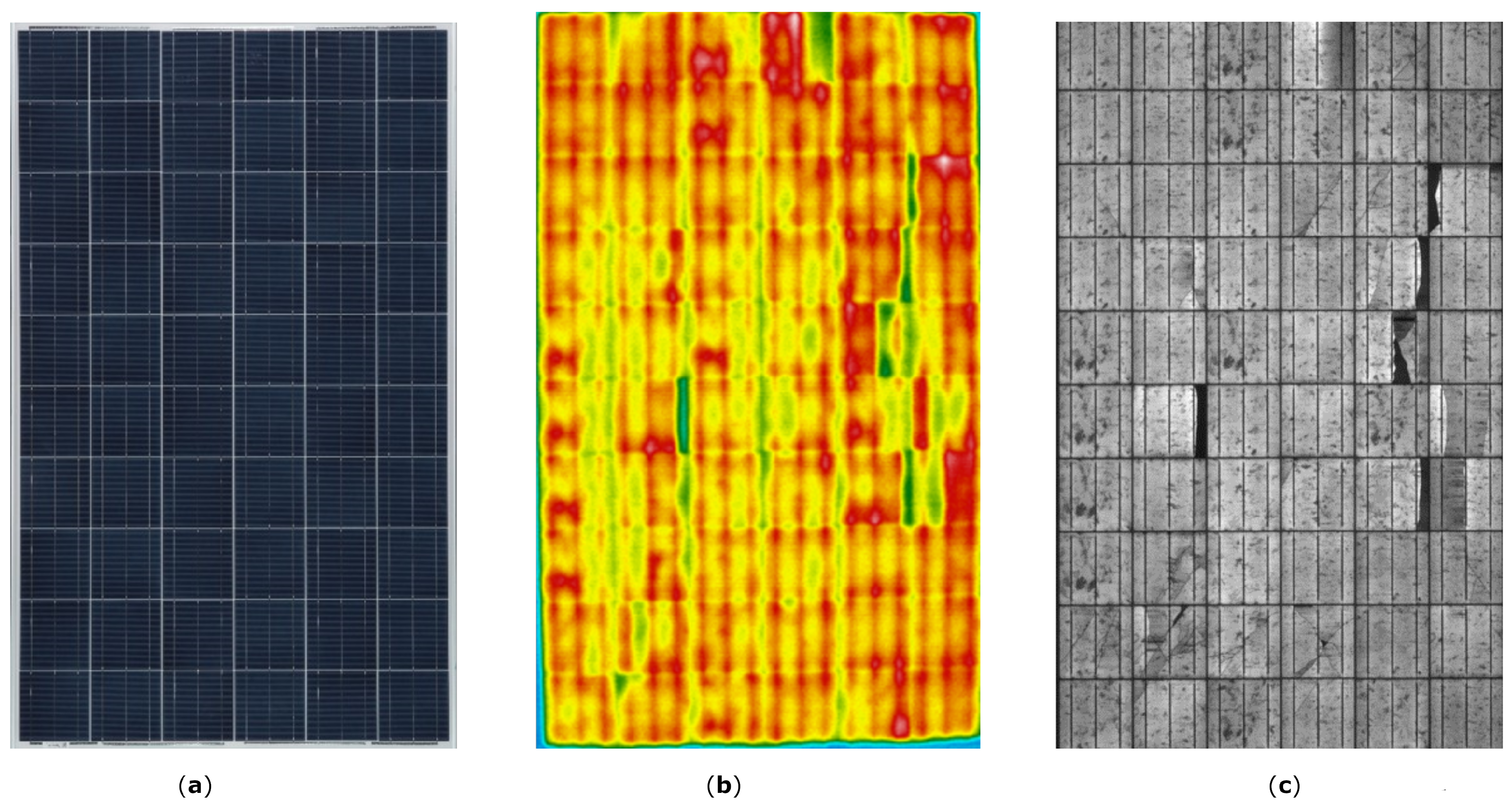
3.5. Defects Detection

Finding defects on the surface of the PV cells is a problem completely related to computer vision. As observed in the bibliography, the most used technique for photographing the images is electroluminescence. The datasets are usually private, but there are some exceptions. We can see in Figure 7 the most used techniques for detecting defects.

Classical approaches as found in [128], which tried to detect defects in the solar modules using image processing techniques. In order to segment the different modules, they used the first derivative of the statistic curve in order to find the division line between each chip. After that, they used another technique, the otsu method, to obtain a binary image. Finally, the algorithm tries to identify the state of the module using the geometry of the resulting image. This algorithm produced interesting results, with a recognition rate of 80% on cracked modules, 95% on fragmented and 99% on good state modules. The recognition was also quite fast. The algorithms were implemented and applied via MATLAB.

Another approach is found in [129]. This method combines the image processing techniques with Support Vector Machines. The dataset featured 13,392 samples of EL images of solar cells. The images are preprocessed in order to reduce spatial noises and to accurately highlight crack pixels in images. After that, binary processing is performed, and finally, the features are extracted from the image. These features are used by different SVMs in order to classify the cells. The results present that the SVM with penalty parameter weighting is the best SVM, with a correct detection rate of 91%, with specificity and accuracy of more than 97%. The experiments were run in MATLAB.

In [130], the author compare Convolutional Neural Networks with SVM. The SVM is trained with data from the ELPV dataset, composed of 2624 EL images of solar cells, obtained by finding the features of the images using different feature descriptors. The CNN used was a pretrained VGG19 with the upper layers changed and trained with the examples. The models were tested with both monocrystalline and polycrystalline modules. The results show that both classifiers were useful for visual inspection, both with an average accuracy of 82.4%. The algorithms were implemented in Python, using Keras for the Neural Network.

The work in [131] presented a similar approach using SVM and CNN. The CNN was composed of two convolutional layers with leaky-relu and max-pooling. The convolutional part was aided by two leaky-relu dense layers and the output layer. The SVM was trained with different features extracted from the images. The dataset was built with 90 images of full-sized commercial modules that were segmented afterward, obtaining 540 cells. The results show similar behavior in both methods, with an accuracy of 98%. The article also tackled unsupervised learning, trying to cluster the images by two features. This resulted in a model that was able to assign the correct label in 66% of cases.The algorithms were implemented in Python, using Tensorflow and OpenCV.

The work found in [132] presents a CNN with 13 convolutional layers, an adaptation of the VGG16 architecture. The dataset was obtained by photographing solar modules of 6 × 12 cells with an EL camera. The network was trained using oversampling and data augmentation in order to reduce the error. The results show that the network performed the best when both oversampling and data augmentation were presented with a Balance Error Rate of 7.73% on binary classification problems of quick convergence. The method was implemented with Keras. The preprocessing was performed with OpenCV.

The authors of [133] present new models that are trained not only with images with cracks but also with corrosion. The images were obtained by photographing modules with the EL technique and performing segmentation afterward, obtaining 5400 images. The models are SVM and CNN. The CNN is composed of two convolutional layers. The SVM parameters are optimized by a grid search. The results show a precision of 99%, an improvement over other methods. The experiments were conducted via Keras and Tensorflow.

A variation of convolutional networks is found in [134]. A multichannel CNN is presented. This network has different convolutional layers for each kind of input. This network also can use inputs of different sizes. After each convolutional layer, a dense layer is applied. Finally, a final dense layer combines all the previous data in order to classify the image. This multichannel CNN improves the feature extraction of single-channel CNNs. The dataset was made by 8301 different EL images of cells. The results show a 96.76% accuracy, much more than the 86% presented by single-channel CNNs. The algorithms were implemented in Python using Keras.

The model presented in [135] is composed of six convolutional layers using different regularization techniques such as batch optimization. The dataset used was the ELPV dataset, with 2624 images. The resulting network is a light architecture that achieved high performance using few parameters with an accuracy of 93%.The experiments were run on Tensorflow.

In order to further improve the results, a new approach is presented in [136]. The authors use Fully Convolutional Neural Networks. An FCNN is a CNN without any dense layer. The model used is the U-net, which has been used previously in biomedical image problems with low data. This dataset was composed of 542 EL images. It is composed of 21 convolutional layers of different sizes. The results show that it was better to accept a slight decrease in the performance in order to improve the speed of the system. The algorithms were implemented in python using Keras and Tensorflow.

Wavelet Transform is used in [137]. This method combines two kinds of WT: Discrete WT and Stationary WT in order to extract textural and edge features from solar cells that have been previously preprocessed. The dataset was composed of 2300 EL images. Finally, two different classifiers are used: An SVM and an FFNN. The best model was the FFNN with 93.6% accuracy, over the 92.6% presented by the SVM.

Another Neural Network used is the Complementary Attention Network in [138]. The CAN is composed of a channel-wise attention subnetwork connected with a spatial attention subnetwork. This CAN can be grouped with any CNN, Fast R CNN [139] being the one chosen by the authors. Two datasets were used, one composed of 2029 images and another of 2129 EL images. The network was used for classification and detection, obtaining an accuracy of 99.17% for classification and a mean average precision of 87.38%. The network was faster and had similar parameter numbers to other commercial methods. The algorithms were implemented using Python.

A very interesting approach is presented in [140]. This method is Deep-Feature-Based, extracting features through convolutional neural networks that are classified afterward for classification algorithms such as SVM, KNN or FNN. The particularity of this system is that it used features from different networks. These features are combined using minimum redundancy and maximum relevance for feature selection. The dataset used was the ELPV dataset, with 2624 images. The selected CNNs for feature extraction are Resnet-50, VGG-16, VGG-19 and DarkNet-19. The best method was found with SVM, selecting 2000 features with an accuracy of 94.52% in two-class classification and 89.63% in four-class classification.

In the

Table 7. Models for detection of faults.

Type	Features	Accuracy	Dataset Size
Image Processing Techniques	Segmentation + obtention of binary image + classification. [128]	from 80% to 99%	—
SVM + Image Processing Techniques	Images are preprocessed and features are extracted from the image. These features are used in an SVM with penalty parameter weighting. [129]	97%	13,392
SVM and CNN	Pretrained VGG19 using different feature descriptors. Similar results for both methods. [130]	82.4%	2624
	CNN is composed of 2 layers using leaky-relu. SVM trained with different features extracted from the images. Similar behavior in both models. [131]	98%	540
	CNN is composed of 2 convolutional layers. SVM parameters optimized by search grid. [133]	96%.	2840
CNN	Thirteen convolutional layers, an adaptation of VGG16. Uses oversampling and data augmentation. [132]	Uses a different measurement	5400
	Multichannel CNN. Accepts inputs of different sizes. Improves the feature extraction of single-channel CNN. [134]	96.76%	8301
	Six convolutional layers. Regulation techniques such as batch optimization. [135]	93%	2624
	Fully Convolutional Neural Network. Pretrained u-net, composed of 21 convolutional layers. [136]	Uses a different measurement	542
	CNN aided by a Complementary Attention Network, composed of a channel-wise attention subnetwork connected with a spatial attention subnetwork. Usable with different CNNs. [138]	99.17%	2300
WT+ SVM and FFNN	Combines discrete WT and stationary WT to extract features and SVM and FFNN to classify them. [137]	93.6%	2029
CNN + SVM, KNN, etc.	Extracts features from different networks, combining them with minimum redundancy and maximum relevance for feature selection. Uses Resnet-50, VGG-16, VGG-19 and DarkNet-19. [140]	94.52%	2624

, a summary of the reviewed models is presented.

4. Discussion

In Section 3, the different IA techniques applied are reviewed for each problem by explaining various important works. In this section, a discussion about the state of the art is performed, summarizing the trends of research and some possible new approaches to consider.

The tracking of the Maximum Power Point has been considered in numerous ways, from traditional and simple methods to methods that use complex technology such as neural networks. The most simple methods still have importance, since a large amount of systems do not need complex MPPT algorithms in order to optimize production. The most complex algorithms are used only in the biggest power plants, where the configuration of the PV arrays, and the large amount of them, makes the process of tracking the Maximum Power Point more complex. Comparing the different techniques presented, it is clear that the most used technologies are the Feed-Forward Neural Networks and the FLC systems (Figure 8). Neural Networks perform better than Logic Systems, but they have some flaws. Neural Networks are highly demanding in terms of computational cost compared with FL systems. The need for large amounts of data is an intrinsic problem of Neural Networks, but it is not as important as it used to be thanks to the high availability of data. Another important problem is the complexity in the optimization of the hyper-parameters, since Neural Networks have a large amount of them. The solution has been found by using optimization algorithms, such as metaheuristics. These algorithms can be used to find the best combinations of parameters or even to find the optimal architecture. As we observed, the problem is still regarded nowadays, since there are ways to improve the efficiency and performance of the most complex systems. To fulfill this objective, more of the newest technologies applied in other sectors should be tried, since as it has been confirmed with the previous works that these kinds of algorithms perform really well on this problem. The FL methods and metaheuristics are usually implemented with MATLAB, but Neural Networks can be implemented with Python as well, using libraries such as Tensorflow [141].

Forecasting is a key problem in PV systems. The estimation of the energy produced by solar plants has been approached as a regression problem in the majority of papers. Due to the availability of data, neural models are highly suitable for solving this problem (Figure 8). The trend is to use the newest neural architectures while optimizing their parameters and their architectures using other methods such as metaheuristics. As observed, an increase in the complexity of the networks improves the results, but this is not the only way of increasing performance. The combination with other systems such as Wavelet Transform increases reliability. Alternative network systems such as Recurrent Networks or Dentritic Networks further improve the results of traditional Neural Networks. This area also has some room for improvement since forecasting is a tricky problem due to its dependence on a large amount of variables. For future research, it would be interesting to test a new combination of parameters, improve the datasets or even try the most innovative technologies that have been used in similar problems. Most of the works are run on MATLAB, but there is an increase in the presence of Python in the latest years due to the Deep Learning Libraries.

Estimating the parameters of the PV models has been conducted with a large number of different algorithms, most of them from the family of metaheuristics (Figure 8). The results are quite similar between them in terms of error (Figure 9); this fact shows that trying to further minimize error is not a worthy effort. The most promising works present a mixture of different metaheuristics, solving the problems or flaws of one metaheuristic by using others. The focus of research should be moved towards finding algorithms with lower computational cost while maintaining the same levels of error. The majority of the methods can be found implemented in MATLAB [141].

Analyzing the state of modules or cells has always been important for optimizing production since damaged modules are not as productive as they should be. As it seen, this problem has been applied mostly to the cell level, segmenting images previously taken of solar modules. Some author have even presented open datasets in order to test the models with a more regular amount of data. The main reason for this problem is related to its nature. The majority of models are trained with unbalanced datasets since the number of damaged modules is usually considerably smaller than good state modules. Another different way of improving the neural models is using pretrained neural networks such as VGG-19 in order to make use of the patterns found in other datasets. Even with their problems, in the bibliography, a considerable amount of models are presented, and they obtain good results (Figure 10); the Convolutional Neural Networks being the most used ones (Figure 8). However, there is a lot to do in this area, mostly, all of the models only use electroluminescence images; the utilization of other techniques such as thermography could bring more information and better results to the models. Another interesting new approach could be fixing the unbalance in the data. Some studies have tried to use simple methods such as flips or rotations, but it is necessary to implement more complex algorithms to generate images that can be used to better train the models. The deep learning methods are mostly implemented with Tensorflow, and OpenCV is usually used for preprocessing the images. MATLAB is used for traditional methods.

5. Conclusions

In this article, the relationship between Artificial Intelligence and Photovoltaic Systems is explained. Numerous problems in this sector can be solved with the use of AI techniques. These techniques present better performance than traditional methods.

Different techniques are applied to the MPPT problem, Neural Networks being the ones which provided better results, even considering their limitations such as high computational requirements or the need for large amounts of data, other approaches involve Fuzzy Logic and Metaheuristics. The forecasting problem is key for PV installations, different models have been created to solve this problem, most of them related to Artificial Neural Networks. These models are usually aided by other algorithms such as metaheuristics to optimize the architecture or the hyperparameters. The estimation of model parameters is also a really important problem, a large variety of metaheuristics have been used to solve this problem with notably good results in terms of error and efficiency. The detection of faults in PV modules has been proved to be vital for the maintenance of PV installations. This is mostly conducted at the cell level and usually only with electroluminescence images. Convolutional Neural Networks are the most used technology for the classification of images, but they need to be empowered with some techniques such as Data Augmentation or Knowledge Transfer.

Research in these areas is not finished, and it is still a hot topic nowadays as it can be seen from the number of publications in recent years; the ways of improving performance and efficiency are still being researched to adapt to every Photovoltaic System. It is observed that one of the most important issues is the quality and quantity of the data. Machine Learning methods need big amounts of data to be able to find patterns for predicting. This issue is even more critical in Deep Learning methods. This research group is addressing this issue for defect detection, creating synthetic EL images of photovoltaic cells to obtain more examples to train models. These images could even be used in other problems of PV systems.

References

1. Adib, R.; Zervos, A.; Eckhart, M.; David, M.E.A.; Kirsty, H.; Peter, H.; Governments, R.; Bariloche, F. Renewables 2021 Global Status Report. In REN21 Renewables Now; 2021; Available online: https://www.iea.org/reports/renewables-2021 (accessed on 10 September 2022).
2. Kampa, M.; Castanas, E. Human health effects of air pollution. Environ. Pollut. 2008, 151, 362–367. [Google Scholar] [CrossRef] [PubMed]
3. Hersbach, H.; Bell, B.; Berrisford, P.; Hirahara, S.; Horányi, A.; Muñoz-Sabater, J.; Nicolas, J.; Peubey, C.; Radu, R.; Schepers, D.; et al. The ERA5 global reanalysis. Q. J. R. Meteorol. Soc. 2020, 146, 1999–2049. [Google Scholar] [CrossRef]
4. Eroğlu, H. Effects of Covid-19 outbreak on environment and renewable energy sector. Environ. Dev. Sustain. 2021, 23, 4782–4790. [Google Scholar] [CrossRef] [PubMed]
5. Danowitz, A. Solar Thermal vs. Photovoltaic. 2010. Available online: http://large.stanford.edu/courses/2010/ph240/danowitz2/ (accessed on 10 September 2022).
6. GreenMatch. Differences Between Solar PV and Solar Thermal; GreenMatch: Copenhagen, Denmark, 2016; Available online: https://www.greenmatch.co.uk/blog/2015/04/solar-panels-vs-solar-thermal (accessed on 10 September 2022).
7. Irena International Renewable Energy Agency. Future of Solar Photovoltaic Deployment, Investment, Technology, Grid Integration and Socio-Economic Aspects; A Global Energy Transformation Paper About IRENA; Technical Report; Irena International Renewable Energy Agency: Abu Dhabi, United Arab Emirates, 2019. [Google Scholar]
8. Markvart, T.; Castañer, L. Principles of Solar Cell Operation. In Practical Handbook of Photovoltaics: Fundamentals and Applications; Elsevier: Amsterdam, The Netherlands, 2003; pp. 71–93. [Google Scholar] [CrossRef]
9. Satpathy, R.; Pamuru, V. Solar PV Power: Design, Manufacturing and Applications from Sand to Systems; Elsevier: Amsterdam, The Netherlands, 2020; pp. 1–493. [Google Scholar] [CrossRef]
10. Yetayew, T.T.; Workineh, T.G. A Comprehensive Review and Evaluation of Classical MPPT Techniques for a Photovoltaic System. In Advances of Science and Technology; Springer: Berlin/Heidelberg, Germany, 2021; Volume 384, pp. 259–272. [Google Scholar] [CrossRef]
11. Pallathadka, H.; Ramirez-Asis, E.H.; Loli-Poma, T.P.; Kaliyaperumal, K.; Ventayen, R.J.M.; Naved, M. Applications of artificial intelligence in business management, e-commerce and finance. Mater. Today Proc. 2021, in press. [Google Scholar] [CrossRef]
12. Alshahrani, A.; Omer, S.; Su, Y.; Mohamed, E.; Alotaibi, S. The technical challenges facing the integration of small-scale and large-scale PV systems into the grid: A critical review. Electronics 2019, 8, 1443. [Google Scholar] [CrossRef] [Green Version]
13. Valer, L.R.; Manito, A.R.; Ribeiro, T.B.; Zilles, R.; Pinho, J.T. Issues in PV systems applied to rural electrification in Brazil. Renew. Sustain. Energy Rev. 2017, 78, 1033–1043. [Google Scholar] [CrossRef]
14. Bosman, L.B.; Leon-Salas, W.D.; Hutzel, W.; Soto, E.A. PV System Predictive Maintenance: Challenges, Current Approaches, and Opportunities. Energies 2020, 13, 1398. [Google Scholar] [CrossRef]
15. Baba, A.O.; Liu, G.; Chen, X. Classification and Evaluation Review of Maximum Power Point Tracking Methods. Sustain. Future 2020, 2, 100020. [Google Scholar] [CrossRef]
16. Eltawil, M.A.; Zhao, Z. MPPT techniques for photovoltaic applications. Renew. Sustain. Energy Rev. 2013, 25, 793–813. [Google Scholar] [CrossRef]
17. Sobri, S.; Koohi-Kamali, S.; Rahim, N.A. Solar photovoltaic generation forecasting methods: A review. Energy Convers. Manag. 2018, 156, 459–497. [Google Scholar] [CrossRef]
18. Chen, M.R.; Chen, J.H.; Zeng, G.Q.; Lu, K.D.; Jiang, X.F. An improved artificial bee colony algorithm combined with extremal optimization and Boltzmann Selection probability. Swarm Evol. Comput. 2019, 49, 158–177. [Google Scholar] [CrossRef]
19. Villalva, M.G.; Gazoli, J.R.; Filho, E.R. Comprehensive approach to modeling and simulation of photovoltaic arrays. IEEE Trans. Power Electron. 2009, 24, 1198–1208. [Google Scholar] [CrossRef]
20. Shapiro, S.; Kouri Kissel, T. Classical Logic. In The Stanford Encyclopedia of Philosophy, Spring 2021 ed.; Zalta, E.N., Ed.; Metaphysics Research Lab, Stanford University: Stanford, CA, USA, 2021. [Google Scholar]
21. Ross, T.J. Fuzzy Logic with Engineering Applications, 3rd ed.; John Wiley & Sons: Hoboken, NJ, USA, 2010. [Google Scholar]
22. Mahmoud, A.M.A.; Mashaly, H.M.; Kandil, S.A.; Khashab, H.E.; Nashed, M.N.F. Fuzzy logic implementation for photovoltaic maximum power tracking. In Proceedings of the 26th Annual Conference of the IEEE-Industrial-Electronics-Society, Nagoya, Japan, 22–28 October 2000; pp. 735–740. [Google Scholar]
23. Hui, J.; Sun, X. MPPT Strategy of PV System Based on Adaptive Fuzzy PID Algorithm. In Life System Modeling and Intelligent Computing Pt I, Proceedings of the International Conference on Life System Modeling and Simulation/International Conference on Intelligent Computing for Sustainable Energy and Environment, Wuxi, China, 17–20 September 2010; Springer: Berlin/Heidelberg, Germany, 2010; Volume 97, pp. 220–228. [Google Scholar]
24. Kottas, T.L.; Karlis, A.D.; Boutalis, Y.S. Fuzzy Cognitive Networks for Maximum Power Point Tracking in Photovoltaic Arrays. Fuzzy Cogn. Maps Adv. Theory Methodol. Tools Appl. 2010, 247, 231–257. [Google Scholar]
25. Stylios, C. Modeling Complex Systems Using Fuzzy Cognitive Maps. Syst. Man Cybern. Part A Syst. Hum. 2004, 34, 155–162. [Google Scholar] [CrossRef]
26. Adly, M.; El-Sherif, H.; Ibrahim, M. Maximum Power Point Tracker for a PV Cell using a Fuzzy Agent adapted by the Fractional Open Circuit Voltage Technique. In Proceedings of the IEEE International Conference on Fuzzy Systems (FUZZ 2011), Taipei, Taiwan, 27–30 June 2011; pp. 1918–1922. [Google Scholar]
27. Altin, N. Interval type-2 fuzzy logic controller based Maximum Power Point tracking in photovoltaic systems. Adv. Electr. Comput. Eng. 2013, 13, 65–70. [Google Scholar] [CrossRef]
28. Karnik, N.; Mendel, J.; Liang, Q. Type-2 fuzzy logic systems. IEEE Trans. Fuzzy Syst. 1999, 7, 643–658. [Google Scholar] [CrossRef] [Green Version]
29. Zadeh, L.A. The concept of a linguistic variable and its application to approximate reasoning—I. Inf. Sci. 1975, 8, 199–249. [Google Scholar] [CrossRef]
30. Mittal, K.; Jain, A.; Vaisla, K.S.; Castillo, O.; Kacprzyk, J. A comprehensive review on type 2 fuzzy logic applications: Past, present and future. Eng. Appl. Artif. Intell. 2020, 95, 103916. [Google Scholar] [CrossRef]
31. MATLAB. Version 7.10.0 (R2010a); The MathWorks Inc.: Natick, MA, USA, 2010. [Google Scholar]
32. Kececioglu, O.F.; Gani, A.; Sekkeli, M. Design and Hardware Implementation Based on Hybrid Structure for MPPT of PV System Using an Interval Type-2 TSK Fuzzy Logic Controller. Energies 2020, 13, 1842. [Google Scholar] [CrossRef] [Green Version]
33. Altin, N. Single phase grid interactive PV system with MPPT capability based on type-2 fuzzy logic systems. In Proceedings of the International Conference on Renewable Energy Research and Applications, ICRERA 2012, Istanbul, Turkey, 18–21 September 2012. [Google Scholar] [CrossRef]
34. Verma, P.; Garg, R.; Mahajan, P. Asymmetrical interval type-2 fuzzy logic control based MPPT tuning for PV system under partial shading condition. ISA Trans. 2020, 100, 251–263. [Google Scholar] [CrossRef]
35. Allouche, M.; Dahech, K.; Chaabane, M. Multiobjective maximum power tracking control of photovoltaic systems: T-S fuzzy model-based approach. Soft Comput. 2018, 22, 2121–2132. [Google Scholar] [CrossRef]
36. Zayani, H.; Allouche, M.; Kharrat, M.; Chaabane, M. T-S fuzzy Maximum Power Point tracking control of photovoltaic conversion system. In Proceedings of the 16th International Conference on Sciences and Techniques of Automatic Control and Computer Engineering, STA 2015, Monastir, Tunisia, 21–23 December 2016; pp. 534–539. [Google Scholar] [CrossRef]
37. Dahmane, M.; Bosche, J.; El-Hajjaji, A.; Davarifar, M. T-S implementation of an MPPT algorithm for photovoltaic conversion system using poles placement and H performances. In Proceedings of the 3rd International Conference on Systems and Control, ICSC 2013, Algiers, Algeria, 29–31 October 2013; pp. 1116–1121. [Google Scholar] [CrossRef]
38. Takagi, T.; Sugeno, M. Fuzzy identification of systems and its applications to modeling and control. IEEE Trans. Syst. Man Cybern. 1985, SMC-15, 116–132. [Google Scholar] [CrossRef]
39. Vaidyanathan, S.; Azar, A.T. Takagi-Sugeno fuzzy logic controller for Liu-Chen four-scroll chaotic system. Int. J. Intell. Eng. Inform. 2016, 4, 135. [Google Scholar] [CrossRef]
40. Azali, S.; Sheikhan, M. Intelligent control of photovoltaic system using BPSO-GSA-optimized neural network and fuzzy-based PID for Maximum Power Point tracking. Appl. Intell. 2016, 44, 88–110. [Google Scholar] [CrossRef]
41. Duman, S.; Yorukeren, N.; Altas, I.H. A novel MPPT algorithm based on optimized artificial neural network by using FPSOGSA for standalone photovoltaic energy systems. Neural Comput. Appl. 2018, 29, 257–278. [Google Scholar] [CrossRef]
42. Sarkar, R.; Kumar, J.R.; Sridhar, R.; Vidyasagar, S. A New Hybrid BAT-ANFIS-Based Power Tracking Technique for Partial Shaded Photovoltaic Systems. Int. J. Fuzzy Syst. 2021, 23, 1313–1325. [Google Scholar] [CrossRef]
43. Naveen; Dahiya, A.K. Implementation and Comparison of Perturb Observe, ANN and ANFIS Based MPPT Techniques. In Proceedings of the International Conference on Inventive Research in Computing Applications, ICIRCA 2018, Coimbatore, India, 11–12 July 2018; pp. 1–5. [Google Scholar] [CrossRef]
44. Arora, A.; Gaur, P. Comparison of ANN and ANFIS based MPPT Controller for grid connected PV systems. In Proceedings of the 12th IEEE International Conference Electronics, Energy, Environment, Communication, Computer, Control: (E3-C3), INDICON 2015, New Delhi, India, 17–20 December 2016. [Google Scholar] [CrossRef]
45. Padmanaban, S.; Priyadarshi, N.; Bhaskar, M.S.; Holm-Nielsen, J.B.; Ramachandaramurthy, V.K.; Hossain, E. A Hybrid ANFIS-ABC Based MPPT Controller for PV System with Anti-Islanding Grid Protection: Experimental Realization. IEEE Access 2019, 7, 103377–103389. [Google Scholar] [CrossRef]
46. Qiao, X.; Wu, B.; Deng, Z.; You, Y. MPPT of photovoltaic generation system using fuzzy/PID control. Electr. Power Autom. Equip. 2008, 28, 92–95. [Google Scholar]
47. Gendreau, M.; Potvin, J.Y. (Eds.) Handbook of Metaheuristics; Springer: New York, NY, USA, 2010. [Google Scholar] [CrossRef]
48. Goldberg, D.E. Genetic Algorithms in Search, Optimization and Machine Learning, 1st ed.; Addison-Wesley Longman Publishing Co., Inc.: Boston, MA, USA, 1989. [Google Scholar]
49. Kulaksiz, A.A.; Akkaya, R. Training data optimization for ANNs using genetic algorithms to enhance MPPT efficiency of a stand-alone PV system. Turk. J. Electr. Eng. Comput. Sci. 2012, 20, 241–254. [Google Scholar] [CrossRef]
50. Kulaksiz, A.A.; Akkaya, R. A genetic algorithm optimized ANN-based MPPT algorithm for a stand-alone PV system with induction motor drive. Sol. Energy 2012, 86, 2366–2375. [Google Scholar] [CrossRef]
51. Larbes, C.; Cheikh, S.M.A.; Obeidi, T.; Zerguerras, A. Genetic algorithms optimized fuzzy logic control for the maximum power point tracking in photovoltaic system. Renew. Energy 2009, 34, 2093–2100. [Google Scholar] [CrossRef]
52. Clerc, M. Particle Swarm Optimization; Wiley: Hoboken, NJ, USA, 2010. [Google Scholar] [CrossRef]
53. Azab, M. Optimal power point tracking for stand-alone PV system using particle swarm optimization. In Proceedings of the IEEE International Symposium on Industrial Electronics, Bari, Italy, 4–7 July 2010; pp. 969–973. [Google Scholar] [CrossRef]
54. Alshareef, M.; Lin, Z.; Ma, M.; Cao, W. Accelerated Particle Swarm Optimization for Photovoltaic Maximum Power Point Tracking under Partial Shading Conditions. Energies 2019, 12, 623. [Google Scholar] [CrossRef] [Green Version]
55. Yang, X.S. Firefly Algorithms for Multimodal Optimization. In Proceedings of the International Symposium on Stochastic Algorithms, Sapporo, Japan, 26–28 October 2009; 5792 LNCS, pp. 169–178. [Google Scholar] [CrossRef] [Green Version]
56. Sundareswaran, K.; Peddapati, S.; Palani, S. MPPT of PV systems under partial shaded conditions through a colony of flashing fireflies. IEEE Trans. Energy Convers. 2014, 29, 463–472. [Google Scholar] [CrossRef]
57. Karaboga, D. An Idea Based on Honey Bee Swarm for Numerical Optimization; Technical Report-tr06; Erciyes University, Engineering Faculty, Computer Engineering Department: Kayseri, Turkey, 2005. [Google Scholar]
58. soufyane Benyoucef, A.; Chouder, A.; Kara, K.; Silvestre, S.; Sahed, O.A. Artificial bee colony based algorithm for Maximum Power Point tracking (MPPT) for PV systems operating under partial shaded conditions. Appl. Soft Comput. J. 2015, 32, 38–48. [Google Scholar] [CrossRef] [Green Version]
59. Bilal, B. Implementation of Artificial Bee Colony algorithm on Maximum Power Point Tracking for PV modules. In Proceedings of the 8th International Symposium on Advanced Topics in Electrical Engineering, ATEE 2013, Bucharest, Romania, 23–25 May 2013. [Google Scholar] [CrossRef]
60. Dorigo, M.; Birattari, M.; Stutzle, T. Ant colony optimization. IEEE Comput. Intell. Mag. 2006, 1, 28–39. [Google Scholar] [CrossRef]
61. Babes, B.; Boutaghane, A.; Hamouda, N. A novel nature-inspired Maximum Power Point tracking (MPPT) controller based on ACO-ANN algorithm for photovoltaic (PV) system fed arc welding machines. Neural Comput. Appl. 2021, 34, 299–317. [Google Scholar] [CrossRef]
62. Moreira, H.S.; Silva, J.L.D.S.; Prym, G.C.; Sakô, E.Y.; dos Reis, M.V.G.; Villalva, M.G. Comparison of Swarm Optimization Methods for MPPT in Partially Shaded Photovoltaic Systems. In Proceedings of the 2nd International Conference on Smart Energy Systems and Technologies (SEST), Porto, Portugal, 9–11 September 2019. [Google Scholar]
63. Telbany, M.E.; Youssef, A.; Zekry, A.A. Intelligent Techniques for MPPT Control in Photovoltaic Systems: A Comprehensive Review. In Proceedings of the 4th International Conference on Artificial Intelligence with Applications in Engineering and Technology, ICAIET 2014, Kota Kinabalu, Malaysia, 3–5 December 2015; pp. 17–22. [Google Scholar] [CrossRef]
64. Oshaba, A.S.; Ali, E.S.; Elazim, S.M.A. PI controller design using ABC algorithm for MPPT of PV system supplying DC motor pump load. Neural Comput. Appl. 2017, 28, 353–364. [Google Scholar] [CrossRef]
65. Habibi, M.; Yazdizadeh, A. New MPPT Controller Design for PV Arrays Using Neural Networks (Zanjan City Case Study). In Proceedings of the 6th International Symposium on Neural Networks, Wuhan, China, 26–29 May 2009; Volume 5552, pp. 1050–1058. [Google Scholar]
66. Veligorskyi, O.; Chakirov, R.; Vagapov, Y. Artificial neural network-based Maximum Power Point tracker for the photovoltaic application. In Proceedings of the 2015 1st International Conference on Industrial Networks and Intelligent Systems, INISCom 2015, Tokyo, Japan, 2–4 March 2015; pp. 133–138. [Google Scholar] [CrossRef]
67. Mlakic, D.; Nikolovski, S. ANFIS as a method for determinating MPPT in the photovoltaic system simulated in MATLAB/Simulink. In Proceedings of the 39th International Convention on Information and Communication Technology, Electronics and Microelectronics, MIPRO 2016, Opatija, Croatia, 30 May–3 June 2016; pp. 1082–1086. [Google Scholar] [CrossRef]
68. Farayola, A.M.; Hasan, A.N.; Ali, A. Efficient photovoltaic mppt system using coarse gaussian support vector machine and artificial neural network techniques. Int. J. Innov. Comput. Inf. Control. 2018, 14, 323–339. [Google Scholar] [CrossRef]
69. Kecman, V. Support Vector Machines—An Introduction; Springer: Berlin/Heidelberg, Germany, 2005; Volume 177, p. 605. [Google Scholar] [CrossRef]
70. Al-Majidi, S.D.; Abbod, M.F.; Al-Raweshidy, H.S. A particle swarm optimisation-trained feedforward neural network for predicting the Maximum Power Point of a photovoltaic array. Eng. Appl. Artif. Intell. 2020, 92, 103688. [Google Scholar] [CrossRef]
71. Avila, L.; Paula, M.D.; Trimboli, M.; Carlucho, I. Deep reinforcement learning approach for MPPT control of partially shaded PV systems in Smart Grids. Appl. Soft Comput. 2020, 97, 106711. [Google Scholar] [CrossRef]
72. Yang, X.S. Bat algorithm: Literature review and applications. Int. J. Bio-Inspired Comput. 2013, 5, 141–149. [Google Scholar] [CrossRef] [Green Version]
73. Pachaivannan, N.; Subburam, R.; Padmanaban, M.; Subramanian, A. Certain investigations of ANFIS assisted CPHO algorithm tuned MPPT controller for PV arrays under partial shading conditions. J. Ambient. Intell. Humaniz. Comput. 2021, 12, 9923–9938. [Google Scholar] [CrossRef]
74. Pachaivannan, N.; Subburam, R.; Ramkumar, U.; Kasinathan, P. Crowded plant height optimisation algorithm tuned Maximum Power Point tracking for grid integrated solar power conditioning system. IET Renew. Power Gener. 2019, 13, 2137–2147. [Google Scholar] [CrossRef]
75. Leone, R.D.; Pietrini, M.; Giovannelli, A. Photovoltaic energy production forecast using support vector regression. Neural Comput. Appl. 2015, 26, 1955–1962. [Google Scholar] [CrossRef] [Green Version]
76. Nageem, R.; Jayabarathi, R. Predicting the Power Output of a Grid-Connected Solar Panel Using Multi-Input Support Vector Regression. Procedia Comput. Sci. 2017, 115, 723–730. [Google Scholar] [CrossRef]
77. Senjyu, T.; Takara, H.; Uezato, K.; Funabashi, T. One-hour-ahead load forecasting using neural network. IEEE Trans. Power Syst. 2002, 17, 113–118. [Google Scholar] [CrossRef]
78. Caputo, D.; Grimaccia, F.; Mussetta, M.; Zich, R.E. Photovoltaic Plants Predictive Model by means of ANN trained by a Hybrid Evolutionary Algorithm. In Proceedings of the World Congress on Computational Intelligence (WCCI 2010), Barcelona, Spain, 18–23 July 2010. [Google Scholar]
79. Gandelli, A.; Grimaccia, F.; Mussetta, M.; Pirinoli, P.; Zich, R.E. Development and validation of different hybridization strategies between GA and PSO. In Proceedings of the 2007 IEEE Congress on Evolutionary Computation, CEC 2007, Singapore, 25–28 September 2007; pp. 2782–2787. [Google Scholar] [CrossRef]
80. Rana, M.; Koprinska, I.; Agelidis, V.G. Forecasting solar power generated by grid connected PV systems using ensembles of neural networks. In Proceedings of the International Joint Conference on Neural Networks, Killarney, Ireland, 12–17 July 2015. [Google Scholar] [CrossRef]
81. Ehsan, R.M.; Simon, S.P.; Venkateswaran, P.R. Day-ahead forecasting of solar photovoltaic output power using multilayer perceptron. Neural Comput. Appl. 2016, 28, 3981–3992. [Google Scholar] [CrossRef]
82. Johansson, E.; Dowla, F.; Goodman, D. Backpropagation Learning for Multilayer Feed-Forward Neural Networks Using the Conjugate Gradient Method. Int. J. Neural Syst. 2011, 2, 291–301. [Google Scholar] [CrossRef]
83. NeuroDimension, Inc. Neurosolutions. Available online: http://www.neurosolutions.com/neurosolutions/ (accessed on 10 September 2022).
84. Li, Z.; Zang, C.; Zeng, P.; Yu, H.; Li, H. Day-ahead Hourly Photovoltaic Generation Forecasting using Extreme Learning Machine. In Proceedings of the IEEE International Conference on Cyber Technology in Automation, Control, and Intelligent Systems (CYBER), Shenyang, China, 8–12 June 2015; pp. 779–783. [Google Scholar]
85. Huang, G.B.; Zhu, Q.Y.; Siew, C.K. Extreme learning machine: A new learning scheme of feedforward neural networks. In Proceedings of the IEEE International Conference on Neural Networks—Conference Proceedings, Budapest, Hungary, 25–29 July 2004; Volume 2, pp. 985–990. [Google Scholar] [CrossRef]
86. Mandal, P.; Madhira, S.T.S.; haque, A.U.; Meng, J.; Pineda, R.L. Forecasting power output of solar photovoltaic system using wavelet transform and artificial intelligence techniques. Procedia Comput. Sci. 2012, 12, 332–337. [Google Scholar] [CrossRef] [Green Version]
87. Mallat, S.G. A Theory for Multiresolution Signal Decomposition: The Wavelet Representation. IEEE Trans. Pattern Anal. Mach. Intell. 1989, 11, 674–693. [Google Scholar] [CrossRef] [Green Version]
88. Park, J.; Sandberg, I.W. Approximation and Radial-Basis-Function Networks. Neural Comput. 1993, 5, 305–316. [Google Scholar] [CrossRef]
89. Capizzi, G.; Napoli, C.; Bonanno, F. Innovative second-generation wavelets construction with recurrent neural networks for solar radiation forecasting. IEEE Trans. Neural Netw. Learn. Syst. 2012, 23, 1805–1815. [Google Scholar] [CrossRef]
90. Wen, Y.; AlHakeem, D.; Mandal, P.; Chakraborty, S.; Wu, Y.K.; Senjyu, T.; Paudyal, S.; Tseng, T.L. Performance Evaluation of Probabilistic Methods Based on Bootstrap and Quantile Regression to Quantify PV Power Point Forecast Uncertainty. IEEE Trans. Neural Netw. Learn. Syst. 2020, 31, 1134–1144. [Google Scholar] [CrossRef] [PubMed]
91. Alzahrani, A.; Shamsi, P.; Dagli, C.; Ferdowsi, M. Solar Irradiance Forecasting Using Deep Neural Networks. Procedia Comput. Sci. 2017, 114, 304–313. [Google Scholar] [CrossRef]
92. Hochreiter, S.; Schmidhuber, J. Long short-term memory. Neural Comput. 1997, 9, 1735–1780. [Google Scholar] [CrossRef] [PubMed]
93. Abdel-Nasser, M.; Mahmoud, K. Accurate photovoltaic power forecasting models using deep LSTM-RNN. Neural Comput. Appl. 2019, 31, 2727–2740. [Google Scholar] [CrossRef]
94. Yao, X.; Wang, Z.; Zhang, H. A novel photovoltaic power forecasting model based on echo state network. Neurocomputing 2019, 325, 182–189. [Google Scholar] [CrossRef]
95. Gallicchio, C.; Micheli, A. Deep Echo State Network (DeepESN): A Brief Survey. arXiv 2017, arXiv:abs/1712.04323. [Google Scholar]
96. Hinton, G.E. A Practical Guide to Training Restricted Boltzmann Machines. In Lecture Notes in Computer Science (Including Subseries Lecture Notes in Artificial Intelligence and Lecture Notes in Bioinformatics); 7700 Lecture N.; Springer: Berlin/Heidelberg, Germany, 2012; pp. 599–619. [Google Scholar] [CrossRef]
97. Jolliffe, I.T. Principal Component Analysis; Springer: Berlin/Heidelberg, Germany, 2002. [Google Scholar] [CrossRef]
98. Davidon, W. Variable Metric Method for Minimization; Technical Report; Argonne National Laboratory (ANL): Lemont, IL, USA, 1959. [CrossRef] [Green Version]
99. Niu, D.; Wang, K.; Sun, L.; Wu, J.; Xu, X. Short-term photovoltaic power generation forecasting based on random forest feature selection and CEEMD: A case study. Appl. Soft Comput. J. 2020, 93, 106389. [Google Scholar] [CrossRef]
100. Breiman, L. Random Forests. Mach. Learn. 2001, 45, 5–32. [Google Scholar] [CrossRef]
101. Behzadian, M.; Otaghsara, S.K.; Yazdani, M.; Ignatius, J. A state-of the-art survey of TOPSIS applications. Expert Syst. Appl. 2012, 39, 13051–13069. [Google Scholar] [CrossRef]
102. Yeh, J.R.; Shieh, J.S.; Huang, N.E. Complementary ensemble empirical mode decomposition: A novel noise enhanced data analysis method. Adv. Adapt. Data Anal. 2011, 2, 135–156. [Google Scholar] [CrossRef]
103. Li, H.; Tan, Q. A BP neural network based on improved particle swarm optimization and its application in reliability forecasting. Res. J. Appl. Sci. Eng. Technol. 2013, 6, 1246–1251. [Google Scholar] [CrossRef]
104. Jiao, B.; Lian, Z.; Gu, X. A dynamic inertia weight particle swarm optimization algorithm. Chaos Solitons Fractals 2008, 37, 698–705. [Google Scholar] [CrossRef]
105. Quan, D.M.; Ogliari, E.; Grimaccia, F.; Leva, S.; Mussetta, M. Hybrid model for hourly forecast of photovoltaic and wind power. IEEE Int. Conf. Fuzzy Syst. 2013. [Google Scholar] [CrossRef]
106. Grimaccia, F.; Mussetta, M.; Zich, R.E. Genetical swarm optimization: Self-adaptive hybrid evolutionary algorithm for electromagnetics. IEEE Trans. Antennas Propag. 2007, 55, 781–785. [Google Scholar] [CrossRef]
107. Koprinska, I.; Wu, D.; Wang, Z. Convolutional Neural Networks for Energy Time Series Forecasting. In Proceedings of the International Joint Conference on Neural Networks (IJCNN), Rio de Janeiro, Brazil, 8–13 July 2018. [Google Scholar]
108. Torres, J.F.; Troncoso, A.; Koprinska, I.; Wang, Z.; Martínez-Álvarez, F. Big data solar power forecasting based on deep learning and multiple data sources. Expert Syst. 2019, 36, e12394. [Google Scholar] [CrossRef]
109. Zhang, T.; Lv, C.; Ma, F.; Zhao, K.; Wang, H.; O’Hare, G.M. A photovoltaic power forecasting model based on dendritic neuron networks with the aid of wavelet transform. Neurocomputing 2020, 397, 438–446. [Google Scholar] [CrossRef]
110. Jiang, T.; Wang, D.; Ji, J.; Todo, Y.; Gao, S. Single dendritic neuron with nonlinear computation capacity: A case study on XOR problem. In Proceedings of the 2015 IEEE International Conference on Progress in Informatics and Computing, PIC 2015, Nanjing, China, 18–20 December 2016; pp. 20–24. [Google Scholar] [CrossRef]
111. Wolff, B.; Lorenz, E.; Kramer, O. Statistical learning for short-term photovoltaic power predictions. Stud. Comput. Intell. 2016, 645, 31–45. [Google Scholar] [CrossRef]
112. Siddiqui, M.U.; Abido, M. Parameter estimation for five- and seven-parameter photovoltaic electrical models using evolutionary algorithms. Appl. Soft Comput. J. 2013, 13, 4608–4621. [Google Scholar] [CrossRef]
113. Opara, K.R.; Arabas, J. Differential Evolution: A survey of theoretical analyses. Swarm Evol. Comput. 2019, 44, 546–558. [Google Scholar] [CrossRef]
114. Glover, F.; Laguna, M. Tabu Search; Springer: New York, NY, USA, 1997. [Google Scholar] [CrossRef]
115. Liang, Y.; Wang, X.; Zhao, H.; Han, T.; Wei, Z.; Li, Y. A covariance matrix adaptation evolution strategy variant and its engineering application. Appl. Soft Comput. J. 2019, 83, 105680. [Google Scholar] [CrossRef]
116. Long, W.; Wu, T.; Jiao, J.; Tang, M.; Xu, M. Refraction-learning-based whale optimization algorithm for high-dimensional problems and parameter estimation of PV model. Eng. Appl. Artif. Intell. 2020, 89, 103457. [Google Scholar] [CrossRef]
117. Zhang, Y.; Ma, M.; Jin, Z. Backtracking search algorithm with competitive learning for identification of unknown parameters of photovoltaic systems. Expert Syst. Appl. 2020, 160, 113750. [Google Scholar] [CrossRef]
118. Saxena, A.; Sharma, A.; Shekhawat, S. Parameter extraction of solar cell using intelligent grey wolf optimizer. Evol. Intell. 2020. [Google Scholar] [CrossRef]
119. Mirjalili, S.; Mirjalili, S.M.; Lewis, A. Grey Wolf Optimizer. Adv. Eng. Softw. 2014, 69, 46–61. [Google Scholar] [CrossRef] [Green Version]
120. Rezk, H.; Arfaoui, J.; Gomaa, M.R. Optimal parameter estimation of solar pv panel based on hybrid particle swarm and grey wolf optimization algorithms. Int. J. Interact. Multimed. Artif. Intell. 2021, 6, 145–155. [Google Scholar] [CrossRef]
121. Li, M.; Li, C.; Huang, Z.; Huang, J.; Wang, G.; Liu, P.X. Spiral-based chaotic chicken swarm optimization algorithm for parameters identification of photovoltaic models. Soft Comput. 2021, 25, 12875–12898. [Google Scholar] [CrossRef]
122. Meng, X.; Liu, Y.; Gao, X.; Zhang, H. A New Bio-inspired Algorithm: Chicken Swarm Optimization. Lect. Notes Comput. Sci. 2014, 8794, 86–94. [Google Scholar] [CrossRef]
123. Yang, X.; Gong, W. Opposition-based JAYA with population reduction for parameter estimation of photovoltaic solar cells and modules. Appl. Soft Comput. 2021, 104, 107218. [Google Scholar] [CrossRef]
124. Rao, R. Jaya: A simple and new optimization algorithm for solving constrained and unconstrained optimization problems. Int. J. Ind. Eng. 2016, 7, 19–34. [Google Scholar] [CrossRef]
125. Sattar, M.A.E.; Sumaiti, A.A.; Ali, H.; Diab, A.A. Marine predators algorithm for parameters estimation of photovoltaic modules considering various weather conditions. Neural Comput. Appl. 2021, 33, 11799–11819. [Google Scholar] [CrossRef]
126. Faramarzi, A.; Heidarinejad, M.; Mirjalili, S.; Gandomi, A.H. Marine Predators Algorithm: A nature-inspired metaheuristic. Expert Syst. Appl. 2020, 152, 113377. [Google Scholar] [CrossRef]
127. Yang, S.; Max, N.; Xie, S.; Li, L.; Zhao, T. Photovoltaic cell model parameter optimization using micro-charge field effect P systems. Eng. Appl. Artif. Intell. 2021, 104, 104374. [Google Scholar] [CrossRef]
128. Nian, B.; Fu, Z.; Wang, L.; Cao, X. Automatic detection of defects in solar modules: Image processing in detecting. In Proceedings of the 6th International Conference on Wireless Communications, Networking and Mobile Computing, WiCOM 2010, Chengdu, China, 23–25 September 2010. [Google Scholar] [CrossRef]
129. Anwar, S.A.; Abdullah, M.Z. Micro-crack detection of multicrystalline solar cells featuring shape analysis and support vector machines. In Proceedings of the 2012 IEEE International Conference on Control System, Computing and Engineering, ICCSCE 2012, Penang, Malaysia, 23–25 November 2012; pp. 143–148. [Google Scholar] [CrossRef]
130. Deitsch, S.; Buerhop-Lutz, C.; Sovetkin, E.; Steland, A.; Maier, A.; Gallwitz, F.; Riess, C. Segmentation of Photovoltaic Module Cells in Uncalibrated Electroluminescence Images. Mach. Vis. Appl. 2018, 32, 84. [Google Scholar] [CrossRef]
131. Karimi, A.M.; Fada, J.S.; Liu, J.; Braid, J.L.; Koyuturk, M.; French, R.H. Feature Extraction, Supervised and Unsupervised Machine Learning Classification of PV Cell Electroluminescence Images. In Proceedings of the IEEE 7th World Conference on Photovoltaic Energy Conversion, WCPEC 2018—A Joint Conference of 45th IEEE PVSC, 28th PVSEC and 34th EU PVSEC, 2018, Waikoloa, HI, USA, 10–15 June 2018; pp. 418–424. [Google Scholar] [CrossRef]
132. Bartler, A.; Mauch, L.; Yang, B.; Reuter, M.; Stoicescu, L. Automated detection of solar cell defects with deep learning. In Proceedings of the 26th European Signal Processing Conference (EUSIPCO), Rome, Italy, 3–7 September 2018; pp. 2035–2039. [Google Scholar] [CrossRef]
133. Karimi, A.M.; Fada, J.S.; Hossain, M.A.; Yang, S.; Peshek, T.J.; Braid, J.L.; French, R.H. Automated Pipeline for Photovoltaic Module Electroluminescence Image Processing and Degradation Feature Classification. IEEE J. Photovoltaics 2019, 9, 1324–1335. [Google Scholar] [CrossRef]
134. Ying, Z.; Li, M.; Tong, W.; Haiyong, C. Automatic Detection of Photovoltaic Module Cells using Multi-Channel Convolutional Neural Network. In Proceedings of the 2018 Chinese Automation Congress, CAC 2018, Xi’an, China, 30 November–2 December 2018; pp. 3571–3576. [Google Scholar] [CrossRef]
135. Akram, M.W.; Li, G.; Jin, Y.; Chen, X.; Zhu, C.; Zhao, X.; Khaliq, A.; Faheem, M.; Ahmad, A. CNN based automatic detection of photovoltaic cell defects in electroluminescence images. Energy 2019, 189, 116319. [Google Scholar] [CrossRef]
136. Balzategui, J.; Eciolaza, L.; Arana-Arexolaleiba, N. Defect detection on Polycrystalline solar cells using Electroluminescence and Fully Convolutional Neural Networks. In Proceedings of the 2020 IEEE/SICE International Symposium on System Integration, SII 2020, Honolulu, HI, USA, 12–15 January 2020; pp. 949–953. [Google Scholar] [CrossRef]
137. Mathias, N.; Shaikh, F.; Thakur, C.; Shetty, S.; Dumane, P.; Chavan, D.S. Detection of Micro-Cracks in Electroluminescence Images of Photovoltaic Modules. SSRN Electron. J. 2020. [Google Scholar] [CrossRef]
138. Su, B.; Chen, H.; Chen, P.; Bian, G.; Liu, K.; Liu, W. Deep Learning-Based Solar-Cell Manufacturing Defect Detection with Complementary Attention Network. IEEE Trans. Ind. Inform. 2021, 17, 4084–4095. [Google Scholar] [CrossRef]
139. Girshick, R. Fast R-CNN. In Proceedings of the 2015 IEEE International Conference on Computer Vision (ICCV), Santiago, Chile, 13–16 December 2015; pp. 1440–1448. [Google Scholar] [CrossRef]
140. Demirci, M.Y.; Beşli, N.; Gümüşçü, A. Efficient deep feature extraction and classification for identifying defective photovoltaic module cells in Electroluminescence images. Expert Syst. Appl. 2021, 175, 114810. [Google Scholar] [CrossRef]
141. Abadi, M.; Agarwal, A.; Barham, P.; Brevdo, E.; Chen, Z.; Citro, C.; Corrado, G.S.; Davis, A.; Dean, J.; Devin, M.; et al. TensorFlow: Large-Scale Machine Learning on Heterogeneous Systems. 2015. Available online: tensorflow.org (accessed on 10 September 2022).
Figure 1. Evolution of the importance of PV sector (adapted from [7]). (a) Evolution of the energy share of PV systems; (b) evolution of the investment in PV energy; (c) evolution of employment in the PV sector.
Applsci 12 10056 g001
Figure 2. Different IV curves. Green circle: Max Power Point; Red Star: Open-Circuit Voltage ( V O C ); Yellow Square: Short-Circuit Current ( I S C ).
Applsci 12 10056 g002
Figure 3. Different techniques for photography modules. (a) Visual spectrum; (b) thermography; (c) electroluminiscence.
Applsci 12 10056 g003
Figure 4. Taxonomy of most used IA method for MPPT.
Applsci 12 10056 g004
Figure 5. Taxonomy of most used IA methods for forecasting.
Applsci 12 10056 g005
Figure 6. Taxonomy of most used metaheuristics for parameter estimation.
Applsci 12 10056 g006
Figure 7. Most used IA method for defect detection.
Applsci 12 10056 g007
Figure 8. Different algorithms for each of the problems. (a) MPPT; (b) forecasting; (c) parameter estimation; (d) defects detection.
Applsci 12 10056 g008
Figure 9. RMSE of the different models for parameter estimation. (a) Single-diode; (b) double-diode.
Applsci 12 10056 g009
Figure 10. Accuracy of the different models for detection.
Applsci 12 10056 g010