
Optimal Control for Cleaner Hybrid Vehicles: A Backward Approach
by
 , , and
Bruno Jeanneret
1,*,† ,
,
Alice Guille Des Buttes
1,2,†,‡,
Alan Keromnes
2,§,
Serge Pélissier
1 and
Luis Le Moyne
2 1
LICIT-ECO7 Lab, Université G. Eiffel, ENTPE, Université de Lyon, F-69675 Bron, France
2
DRIVE EA1859 Lab, Université de Bourgogne, F-58027 Nevers, France
*
Author to whom correspondence should be addressed.
†
These authors contributed equally to this work.
‡
Current address: INSA-Toulouse, 135 Avenue de Rangueil, F-31077 Toulouse, France.
§
Current address: IRCER Lab, UMR CNRS 7315, Université de Limoges, F-87000 Limoges, France.
Appl. Sci. 2022, 12(2), 578; https://0-doi-org.brum.beds.ac.uk/10.3390/app12020578
Submission received: 17 November 2021
/
Revised: 20 December 2021
/
Accepted: 22 December 2021
/
Published: 7 January 2022
(This article belongs to the Special Issue Energy Management of Hybrid Electric Vehicles 2021)
Abstract
:This work presents an application of the optimal control theory to find trade offs between fuel consumption and pollutant emissions (CO, HC, NOx) of sustaining hybrid vehicles. Both cold start and normal operations are considered. The problem formulation includes two state variables: battery state of energy and catalyst temperature; and three control variables: torque repartition between engine and motor, spark advance, and equivalence ratio. Optimal results were obtained by delaying the first engine crank after the urban part of the mission. The results show that a quick catalyst light off is performed. Once the catalyst is primed, special control parameters values are adopted to operate the engine.
1. Introduction
The Emissions Database for Global Atmospheric Research (EDGAR) is a global greenhouse gas inventory developed by the Joint Research Centre at the European Commission [1]. Recent results show that global fossil CO2 emissions increased by 1.9% in 2018 and 0.9% in 2019. The transportation sector is responsible for 21% of these emissions, with a slightly increasing trend. Several of the main CO2 emitting countries reduced their emissions in 2019 compared to 2018, including the European Union (by 3.8%), United States (by 2.6%), Japan (by 2.1%), and Russia (by 0.8%). Conversely, China (3.4%) and India (1.6%) increased their emissions in 2019, representing 30.3%, and 6.8% of the global total, respectively.
The effect of global warming is particularly evident when you walk through the alps; the retreat of the glaciers is impressive. A recent study conducted by Vincent et al. [2] shows that for the Intergovernmental Panel on Climate Change (IPCC) scenario RCP 4.5, in which greenhouse gas emissions decline after 2050 and concentrations stabilize towards the end of the 21st century, the Argentière glacier might disappear towards the end of the 21st century and the Mer de Glace surface area could decrease by 80%. The glaciers of the Alps will then almost all disappear within 80 years.
However, the transportation sector is not only responsible for a large part of global warming effects; it also impacts air pollution, which affects health. In 2018, the European Environment Agency estimated that nitrogen dioxide (NO2) was linked to 54,000 premature deaths across the 27 EU member states and the United Kingdom. Particulate matter and black carbon also affect human health, from impairing the respiratory system to causing premature death [3,4]. In the case of France, the road transportation sector is responsible for 57% of total NOx emission [5]. Globally, fleet renewal leads to a decrease in emissions despite traffic growth. Emissions of particulate matter PM10, PM2.5, PM1.0, and black carbon (BC) from the road transportation sector include particulate from vehicle exhausts. It also encompasses PM from wear and tear on roads and certain vehicle components such as tires and brakes. The road sector is responsible for 15 to 20% of total PM emissions depending on their size, and 50% of black carbon is emitted by the combustion of fossil fuels in the vehicles.
“Is it really the end of internal combustion engines and petroleum in transport?” asked Pr Kalghatgi [6]. Obviously, the balance is very unfavorable to fossil fuels. Helmers et al. [7] made a life cycle assessment (LCA) of electric vehicles (EVs) versus conventional vehicles (CVs) using the ReCiPe characterization method. This method captures 18 impact categories and a single score endpoint. The results show that EVs are very advantageous with respect to climate change impacts. This is especially true when using all options, such as green electricity charging, battery production under green electricity supply, and battery second use. However, the study also reveals disadvantages of electric cars in several impact categories (e.g., human and freshwater toxicity, freshwater eutrophication, mineral resource depletion, and agricultural and urban land occupation).
Nevertheless, we have to be aware that at the time of writing, the share of renewables in global electricity generation jumped to nearly 28% in Q1 2020 from 26% in Q1 2019. The increase in renewables came mainly at the cost of coal and gas, though those two sources still represent close to 60% of the global electricity supply [8]. Although this share will have to increase in the future to limit global warming [9], a majority of our electricity still comes from fossil fuels.
Even if conventional vehicle will be replaced by all electric vehicle in the future, we must keep working on the combustion engine. There is still room for improvement. Leach et al. [10] reviewed new developments that can improve engine efficiency. Among these, we can cite increasing the expansion ratio with respect to the compression ratio, reducing pumping work losses and throttle pressure drop with exhaust gas recirculation, downsizing, supercharging, etc. Furthermore, during this transition phase, hybrid electric vehicles (HEVs) will play a key role [11]. In this context, it is of primary importance to find virtuous compromises between energy saving and pollutant emissions.
Some experiments conducted in our lab show that focusing on fuel economy can induce extra pollution. This is the case for eco-driving research, as shown by Mensing et al. in [12]. In this study, the authors compared two eco-driving strategies on a hybrid vehicle equipped with an internal combustion engine controlled by a standard ECU (electronic control unit). The strategy that minimized fuel consumption runs at full throttle during part of the driving cycle. A slight enrichment of the fuel to air mixture occurs in this part of the cycle in order to reduce high chamber temperatures. This induces high CO and HC emissions.
Furthermore, special control parameters are adopted during cold start to shorten this stage, which emits a large amount of pollutants for several reasons: firstly, the catalyst is not efficient until it reaches its light-off temperature [13,14,15]. Secondly, the HC concentration at low chamber temperatures is high due to flame quenching and misfires [16,17]. As a consequence, special control parameters of the ICE are used during this period. Usually, late ignition regarding optimal values is employed in order to bring more heat to the after-treatment system [18,19]. In this context, the energy management strategy must take into account the engine control parameters if we want to consider both fuel economy and pollutant emissions.
The article is mainly based on works by Mrs. Guille des Buttes during her PhD [20] and pursues new developments on those works. Optimal control theory was adopted to show how the control parameters of the engine are actuated. A trade-off between fuel consumption and pollutant emissions during both cold start and normal operation of the engine was achieved. This work differs from what is usually described in the literature because here no arbitrary choices were made to find these compromises. The article is outlined as follow: after explaining the methodology in detail in Section 2, we present the results in Section 3. Section 4 is a discussion of the results. In the last section, we briefly summarize our main results.
2. Materials and Methods
2.1. Base Line Application Object
The reference vehicle used in the present study is a parallel hybrid whose architecture is described in Figure 1. It comprises an internal combustion engine (ICE) and an electric motor (EM) coupled by a gear, a battery, and a power converter, two clutches (allowing fully electric and hybrid operation), a gearbox, and a final drive connected to the wheels. Table 1 gives the characteristics as well as the model used to simulate each of the main components.
2.2. Optimal Control Theory
In 2015, Zhang et al. [21] made a comprehensive analysis of energy management strategies (EMS) for HEV. The review, based on bibliometrics, analyzes almost 600 articles from the view of control problems. They classified EMS as rule-based strategies or optimization-based strategies; the latter was subdivided between real time and global. Two methods retain attention: dynamic programming (DP) and indirect methods, which encompass the well known Pontryagin maximum principle (PMP). They concluded that DP is very robust but must be solved numerically by approximations. The approach also suffers from Bellman’s “curse of dimensionality” and is restricted to small state dimensions. Therefore, there is a trade-off between convergence of the result and computational load. On the other side, PMP reduces constrained global optimization into local Hamiltonian minimization, but the underlying differential equations are often difficult to solve due to strong non-linearity and instability [22].
The review from Zhang et al. not only focuses on the optimal methods that were used in the literature, but also on the objective function studied: 75% of the research articles concerned fuel economy and only a quarter focused on emissions. Moreover, they do not mention any articles taking into account the engine control parameters. They suggest that future trends of EMS should include multi-objective strategies which combine energy conservation (fuel economy), environmental impact (pollutant emissions), safety (fault tolerance and component reliability), and comfort (driveability).
2.3. Model Structure
The core of the methodology lies in the model of the engine and its after-treatment system. Dynamic programming was used and, in our case, involved two state variables: the first representing the state of energy of the battery and the second representing the catalyst temperature. There were three control parameters in our algorithm, one being the intake manifold pressure that drives engine torque and the two others being the relative spark advance, , and the air to fuel equivalence ratio, .
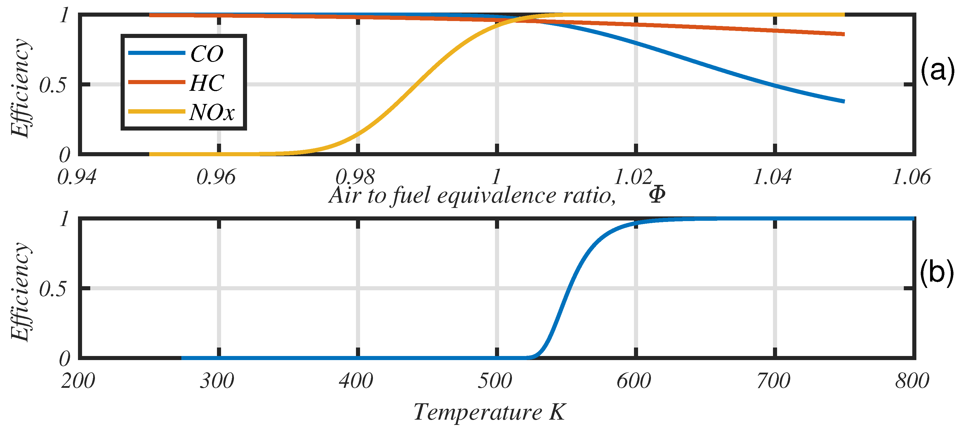
The vehicle dynamics and the resulting power demand are modeled using a backward approach. The velocity as a function of time is known in advance and this driving cycle corresponds to a necessary torque at the wheels to overcome the inertia of the vehicle as well as the resistive forces acting on it. The mechanical transmission components have constant efficiencies and the engine speed is saturated to its idle speed. All numerical values of the equations and parameters are presented in [23]. The three-way catalyst (TWC) efficiency model has also been described in [23]. This latter model uses two Wiebe functions to model global efficiency:
- As a function of catalyst temperature, ;
- Regarding the air to fuel equivalence ratio, .
In which x represents the different species: CO, HC, and NOx. Figure 4 presents the shape of the curves.
Finally, the engine model, fully described in [24] (equations, parameters values and measurements), comprises the following different parts:
- CO, HC, and NO tailpipe concentration;
- Fuel flow behavior;
- Brake torque model;
- Exhaust temperature depending on operating parameters.
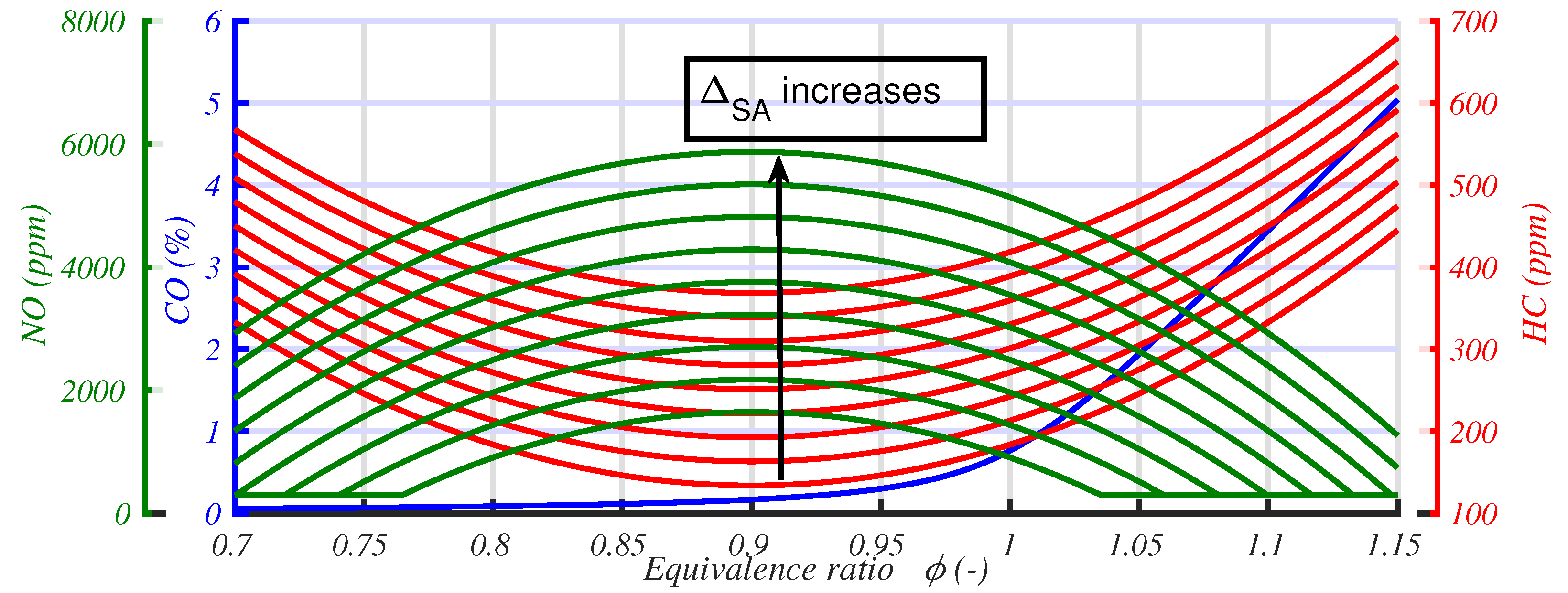
For clear comprehension of the results, it is mandatory to recall the equations of engine emissions (see Equations (2)–(4)) and illustrate their shape for an arbitrary operating point (N = 2000 rpm; = 0.9 bar) and various relative spark advance values (see Figure 5). A zero relative spark advance () is optimal regarding engine efficiency; however, emission models are defined in absolute spark advance with the following relationship: .
2.4. Problem Formulation
The optimal control problem is given by Equation (5), which is the weighted sum of pollutant emissions and fuel consumption.
Both fuel consumption and pollutant emissions show extremely different orders of magnitude. To normalize them, we consider the EURO6 emission levels and the CO2 target value (expressed in l/100 km) of the Corporate Average Fuel Economy for cars (CAFE regulation, see [25]). These values are presented on Table 2.
The system is subjected to the following constraints:
- The battery state-of-charge (SOC) lies between 20% and 80% in order to avoid any damage;
- SOC variation is limited by the maximum and minimum battery currents;
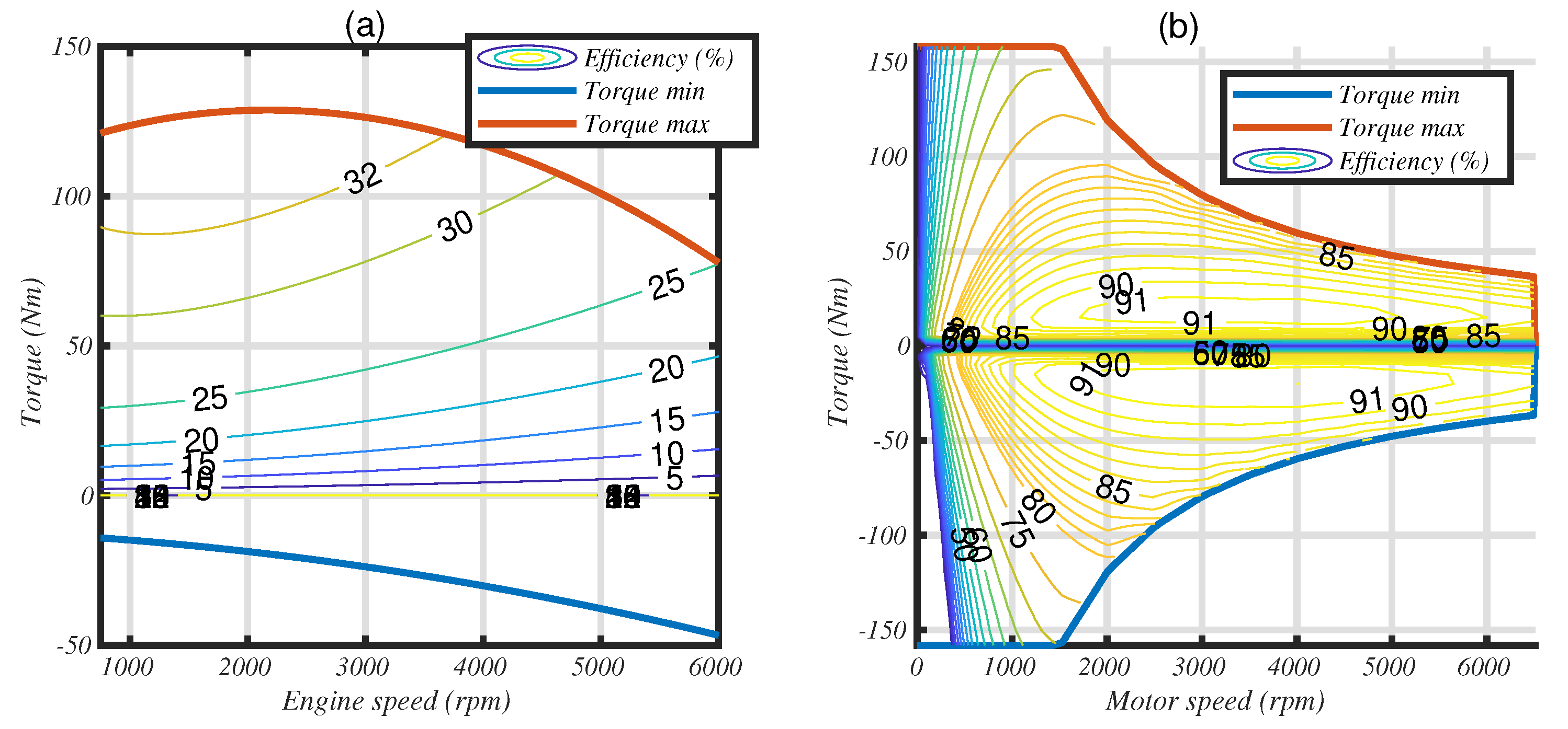
- The torque of the ICE (respectively EM) is limited by torque vs speed curves in both traction and friction (respectively regenerative) modes, see Figure 6;
- Catalyst temperature can vary freely during the driving cycle.
The initial and final values of the state variables are given by the boundary conditions:
- Initial and final values of the SOC are equal to 50% to ensure a fair comparison of scenarios without energy transfers from the battery to the tank, as the reference vehicle is a self-charging hybrid;
- The initial catalyst temperature is set to ambient;
- The final catalyst temperature is unconstrained; of all possible temperatures corresponding to a null electrical energy balance, the one that minimizes the objective function is selected.
2.5. Algorithm Overview
Dynamic programming is based on Bellman’s principle of optimality [26]. The core of the algorithm was developed with MATLAB® and is presented in detail in Appendix A. It consists of calculating the cost-to-go matrix of the three-dimensional graph. This graph is defined by the time of drive cycle in the X-axis, the battery state of charge in the Y-axis, and the TWC temperature in the Z-axis. The optimal policy can only be calculated when the entire drive cycle has been performed, so the graph has to be stored in RAM or HDD in this implementation. As we consider three control variables, the lowest value of the objective function can be obtained by any of the combinations of the control variables, which considerably increases the size of the problem. Hopefully, this minimization can be done at each time step. Finally, the optimal policy is calculated with a backward approach, by breaking the decision problem into smaller subproblems.
2.6. Problem Discretization
In the most general form of solving a dynamic programming problem, the solution space typically needs to be discretized and interpolation is used to evaluate the cost-to-go function between the grid points. This produces rounding errors if the discretization is not fine enough [27,28].
The size of the problem is constrained as it must fit in the 256 GB of memory available in our computer and run in a reasonable time. In this context, some compromises have to be made given the combinatorial increase in the dimensions of the system.
2.6.1. Battery Energy Step
The battery state of energy () is the first state variable. Starting with the variation in SOE between two step times, we can calculate the battery power, and by reversing the electric motor loss map, the mechanical power required at the motor shaft. In a backward approach, the power required to drive the vehicle is perfectly known. Accordingly, we can calculate the engine power and torque. The engine model comprises three control variables: intake pressure, relative spark advance, and air to fuel equivalence ratio. By mixing equations, we calculate the necessary intake pressure that satisfies the required engine torque for the particular values of spark advance and equivalence ratio. With this procedure, we eliminate the rounding errors between intake pressure and torque and there is no need to interpolate. Another important fact is that the all-electric mode is obtained by construction of the graph without rounding errors; indeed, the lower SOE bound, which represents the maximum discharge of the battery, is defined by the all-electric mode of the vehicle.
A parametric study was conducted on the battery net energy step size. The calculations were conducted with a step time of 1 s, for a stoichiometric equivalence ratio () and an optimal spark advance. Only fuel was optimized, that is (see Equation (5)).
We observed the deviation in fuel and emissions compared to a reference strategy where the discretization is very fine. We also constructed a form factor that describes how the different strategies differ from the reference one. This form factor is defined as follows (see Equation (6)):
Deviation in fuel consumption or emissions are very small for all values of battery energy step, as shown in Table 3. The form factor also stays very stable. This allows us to use a relatively large discretization step without affecting the accuracy of the calculations.
2.6.2. Catalyst Temperature STEP
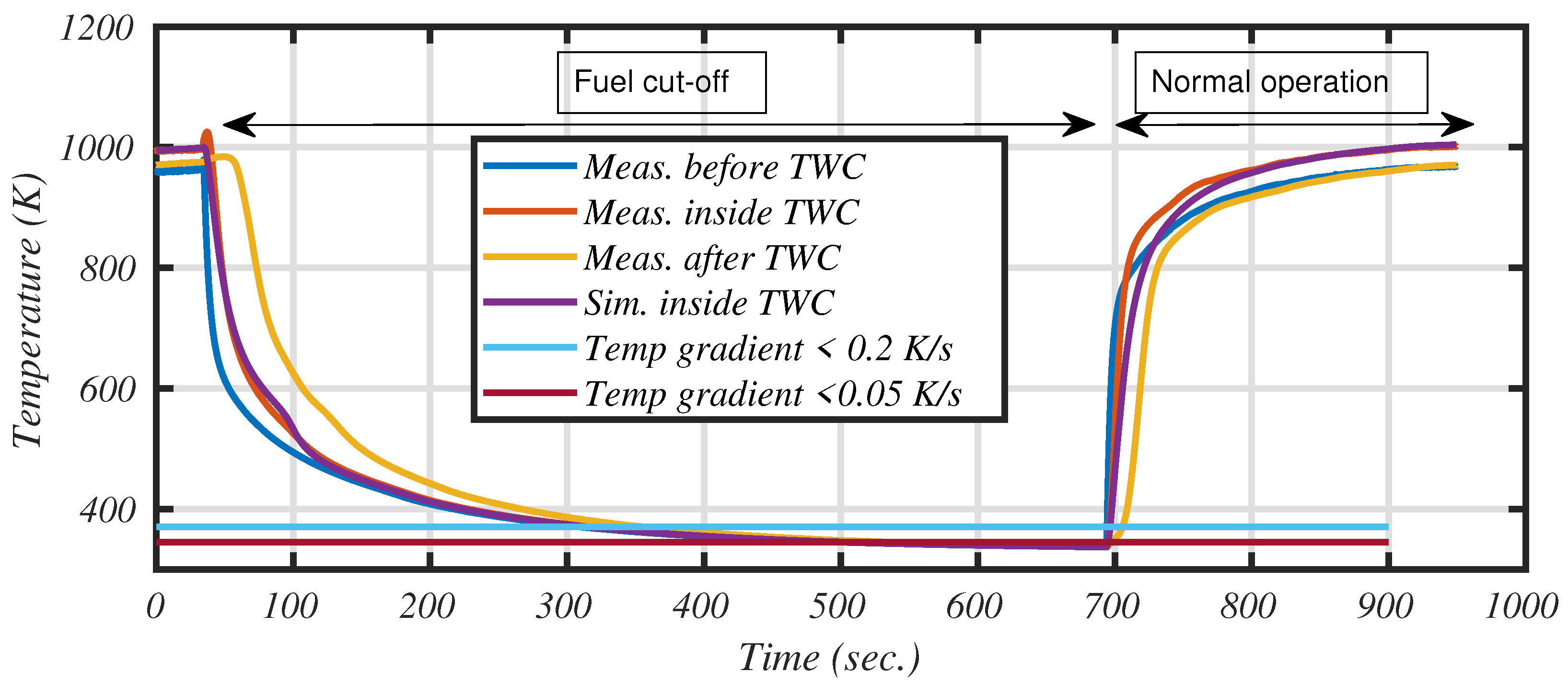
The second state variable is the catalyst temperature, as it drives overall efficiency and the associated emitted pollutants. The catalyst monolith temperature varies continuously despite the discrete control variable. In order to match the temperature discretization and limit the rounding errors, the mesh has to be very fine, especially between the ambient and light-off temperatures, where the catalyst efficiency is low. For example, Figure 7 represents a cooling period with fuel cut-off followed by constant operation at 2500 rpm, 38% throttle. We see that the gradient’s temperature falls below 0.2 K/s at around 370 K and below 0.05 K/s at 345 K. Catching cooling behaviors is particularly important for hybrid applications where engine can be off during long periods of time, thus deactivating the after-treatment system.
Previous work [23] shows that a step of 0.2 K was mandatory for a time step of 1 s. Indeed, as can be seen in Figure 7, the cooling speed is lower than 0.2 K/s near ambient temperature. To continue to account for air cooling during the cold start phase while reducing the size of the state vector, it is possible to change the time step used for the calculation. A cooling rate of 0.2 K/s corresponds to 0.4 K for a duration of 2 s. This increase in the time step reduces the number of calculations to be carried out by half, with a corresponding reduction in the maximum amount of memory used to calculate the graph.
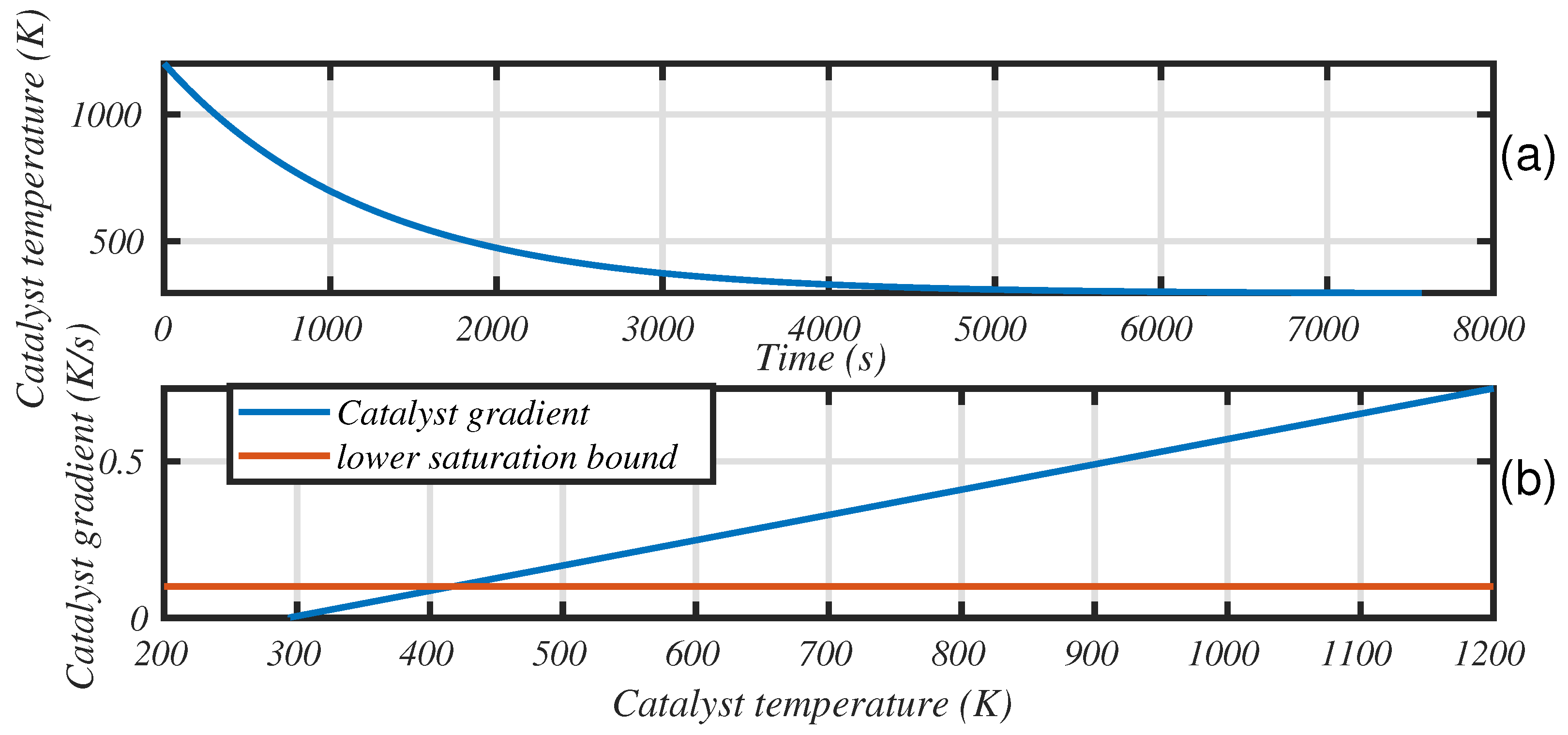
Another way of solving this problem lies in the fact that we need precision under catalyst light-off temperature, but as soon as the catalyst is primed, we can increase the temperature step. Thus, as an alternative, a non-regular discretization was chosen. This allows the calculation of the model with a step time of 1 s. A linearly increasing temperature gradient that begins at 0.1 K/s and that matches natural cooling was chosen (see Figure 8).
2.6.3. Time Step
Increasing the time step has an effect on the precision of the calculations. The power demanded from the wheel by the cycle is calculated numerically from the velocity and acceleration vectors. To increase the time step, a new velocity vector is determined by interpolation from the velocity profile of the cycle sampled at 1 s. This new vector is used to evaluate the acceleration of the vehicle and thus the inertial forces.
In order to quantify the variation of the power profile as a function of the time step, the traction energy required to move the vehicle is calculated. This corresponds to the integral of the positive power over the whole cycle (determined by means of a trapezoidal numerical integration) divided by the distance traveled. The traction energies after resampling are compared to the reference corresponding to a time step of 0.1 s. Table 4 summarizes the results.
From Table 4, we can conclude that a time step of 1.0 s presents an error less than 1% and constitutes a good compromise between calculation time and precision.
2.6.4. Selected Optimization Parameters
In this section we have discussed the influence of the discretization of the system. As a result, two groups of optimization parameters are retained in this study:
- Group A:
- −
- The time step is 1 s;
- −
- The SOE step is 1500 J;
- −
- The temperature step varies linearly to limit grid errors during the natural cooling of the catalyst.
- Group B:
- −
- The time step is 2 s;
- −
- For the SOE grid, the step is 3000 J;
- −
- The temperature step is fixed. It increases from 0.2 K to 0.4 K, but the cooling rate stays at 0.2 K/s due to the increased time step.
Under these assumptions, the Group B scenario consumes more RAM than the Group A scenario, all other things being equal. Finally, for the ignition timing and air to fuel equivalence ratio, the steps studied will be specified in the following sections.
3. Results
3.1. Consumption Centered Scenario
The best efficiency area lies at an equivalence ratio of = 0.97 (the model is from [29] and is fully developed in [24]). However, the efficiency improvement is less than 2% between = 0.97 and = 1.0, and the value = 0.97 emits a very large amount of NOx (the NOx conversion efficiency falls from 100% to almost 0 in this narrow window; see Figure 4). Therefore, this strategy will not be studied.
The consumption centered scenario is calculated for stoichiometric combustion and an optimal spark advance. Results are presented in Table 5.
These values must be compared to the CO2 emissions targets for cars, established at 95 g CO2/km, and the EU current regulations (EURO6) as given in Table 2.
The first analysis shows that even very efficient sustaining hybrid drive trains have difficulties achieving the new regulations in term of CO2 emissions. In this example, the WLTC driving cycle consumes 20% more than its NEDC predecessor. This new cycle must be welcomed, as it is closer to real-world conditions, but it makes the 95 g CO2/km target all the more difficult to achieve.
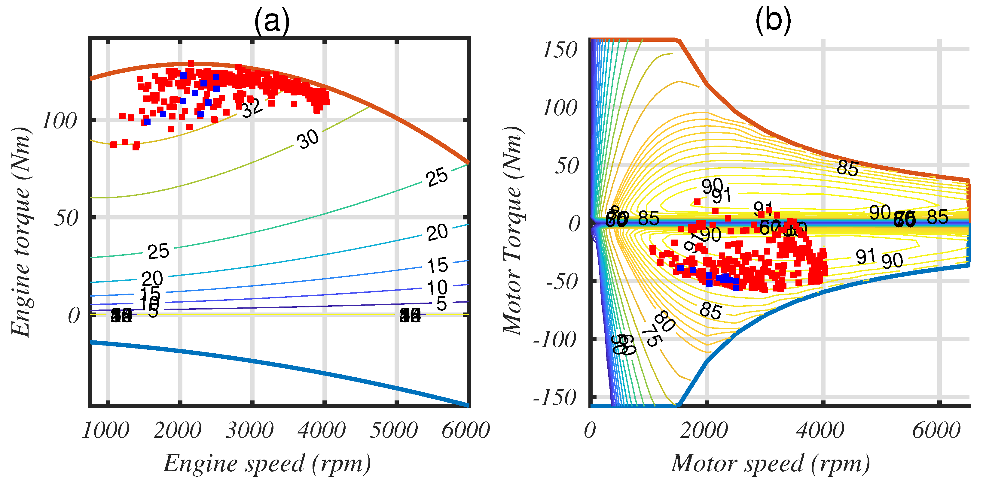
Figure 9 shows the efficiency maps of ICE and EM (the points correspond to the hybrid mode only; i.e., we do not represent the electrical machine operating points in all-electric mode).
Firstly, we notice that the best efficiency of the engine used in this article is 32% (which corresponds to a BSFC of 245 g/kWh). Better efficiency is currently possible; for example, a minimum BSFC value of 225 g/kWh is obtained with the Atkinson cycle engine that equips the Prius II (Model/Year 2004, see [30]).
Secondly, we notice that the engine works in its best efficiency area, which is quite normal for this strategy. This is also the case for the electric machine.
A supplementary degree of freedom that is not in the scope of this work is the gearbox. Neither the number and ratios of the gears, nor the instances where the gears change have been optimized. This latter option can bring improvements in fuel consumption without sacrificing vehicle driveability [31]. The five gear ‘20DP42’ gearbox used in this study is quite old and we currently see automated gearbox with six, seven, and even eight gears in today’s vehicle. This greatly improves fuel consumption, especially in highway mode [32].
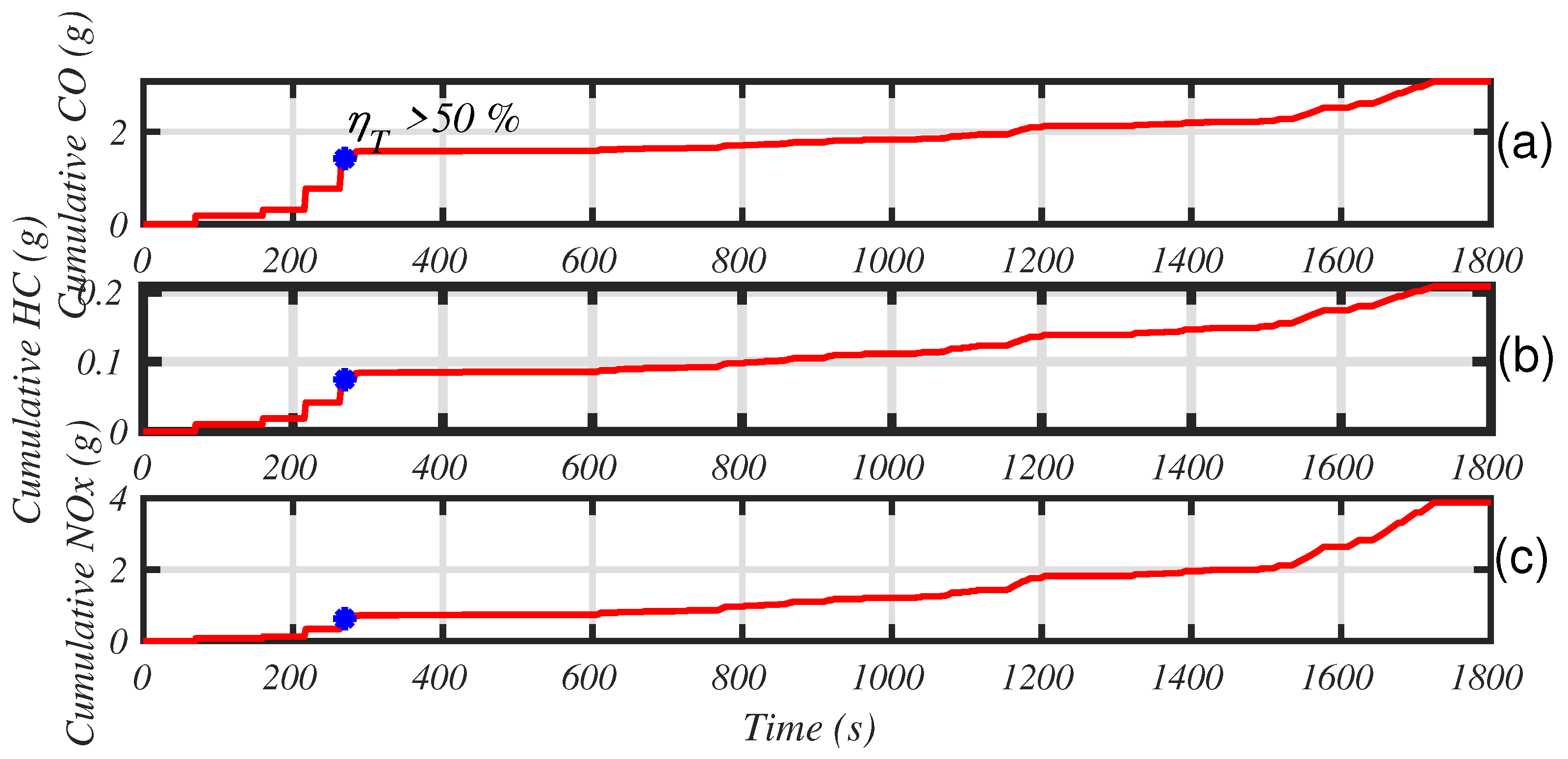
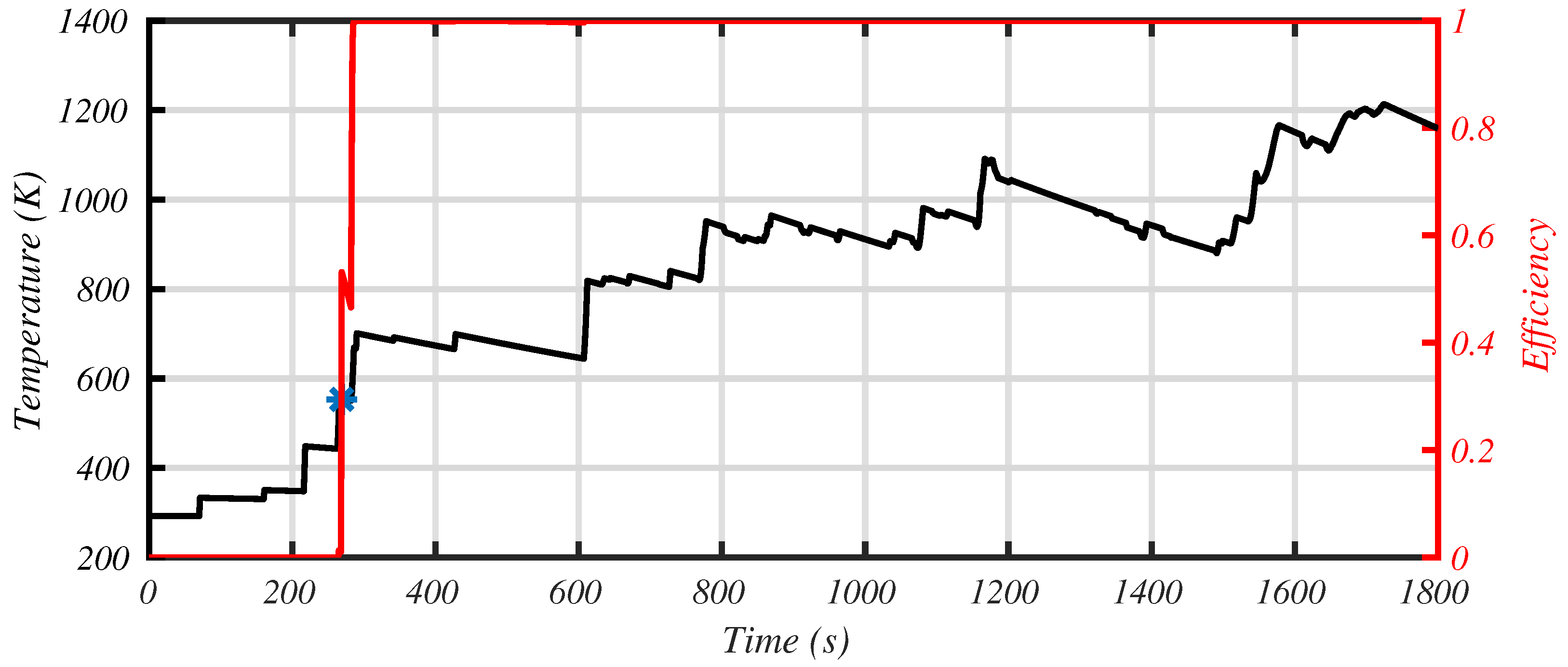
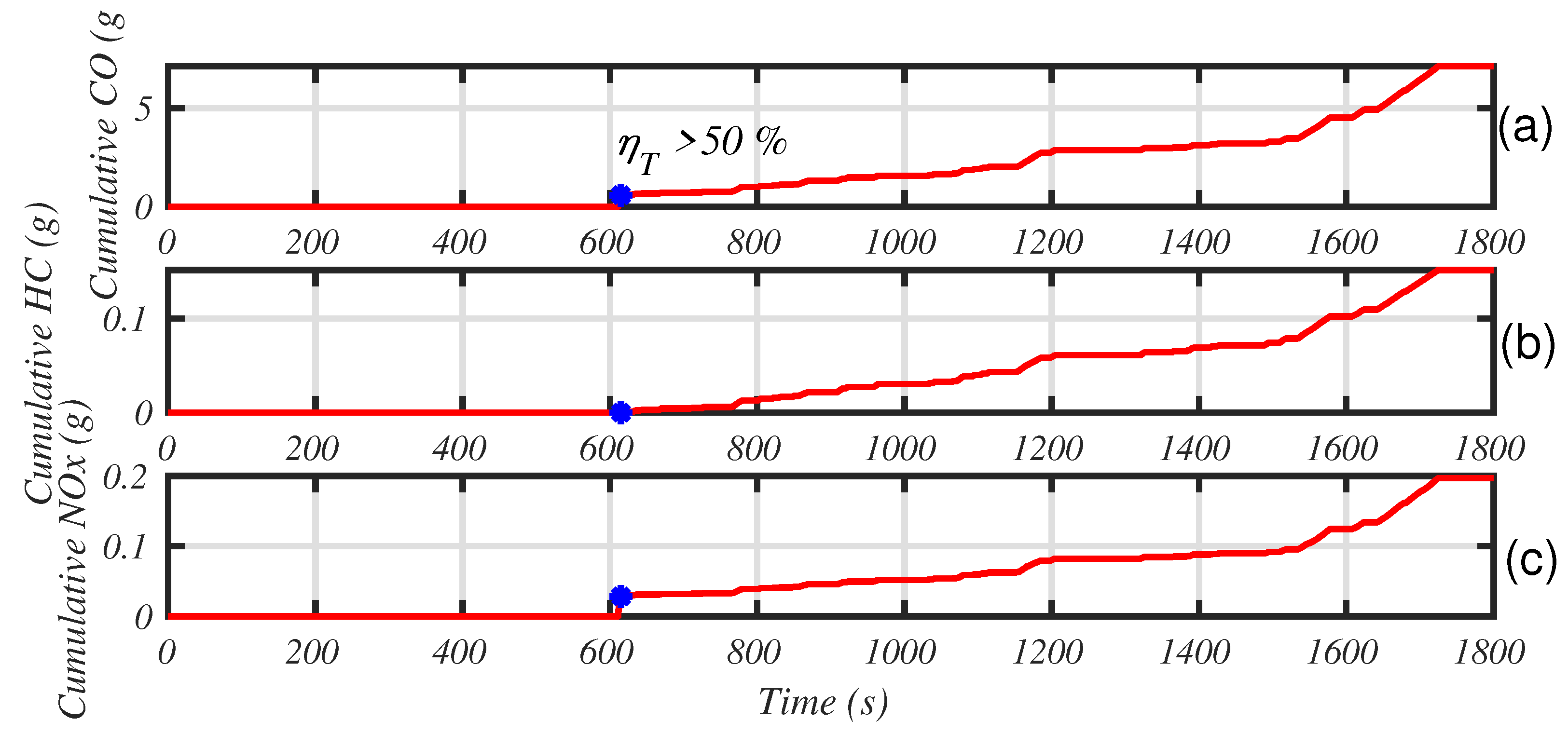
In term of emissions, CO or HC are very low compared to the current regulations. However, the NOx level is almost three times higher than EURO6 limit. Figure 10 shows the cumulative emissions, while Figure 11 shows the temporal evolution of the catalyst temperature and efficiency.
Before the catalyst light off, almost half of the total amount of CO and HC has already been emitted. For the total NOx, 15% has already been dispersed in the environment.
Catalyst is primed after 250 s (the time when the efficiency exceeds 50%, symbolized with blue stars in Figure 10 and Figure 11), during which half of the urban part of the driving cycle has been performed. Between 250 and 600 s, the catalyst is cooling and is not far from being inefficient due to low temperature (light-off temperature is 550 K in our model). This can happen in real usage (stops or congested areas, for example) and must be managed by the engine ECU.
3.2. Emission-Centered Scenario
In this section, we consider a scenario in which the weighting parameters are equals (, see Equation (5)) and the Group A hypothesis concerning the optimization parameters is selected.
An analysis of the use of RAM on the computing machine has shown that the implementation of the method does not allow the use of more than 16 values of advance and/or equivalence ratio without reaching the limits of the available memory (256 GB) for the Group A parameters. Therefore, four values for the air to fuel equivalence ratio and four values for the relative spark advance are considered.
Table 6 summarizes the discretization steps used in Section 3.2.
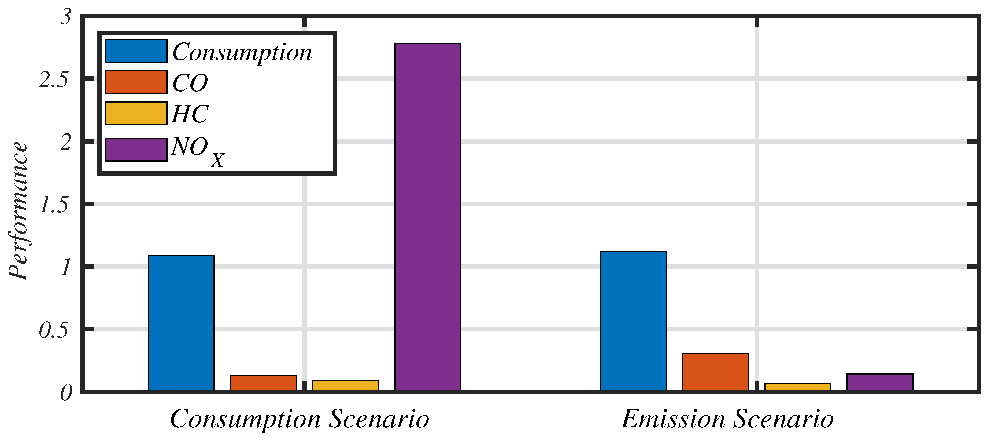
Global results are presented in Table 7 and a comparison with the consumption-centered scenario is drawn in Figure 12 for the WLTC driving cycle. In this drawing, the performance index is represented by the normalized value of the component. For example, the performance index of the fuel is: (see Equation (5)).
Aggregated results show that, whatever the driving cycle considered, a small increase in fuel consumption (between 3% to 5%) allows a great reduction in NOx emission (divided by a factor 20), thus passing the EURO6 rules (0.060 g/km). One can also notice that CO emissions increase, but still stay three times lower than EU limits.
Let us take a deeper look at the results. Figure 13, Figure 14, Figure 15, Figure 16 and Figure 17 shows the temporal evolution of key variables in the WLTC driving cycle.
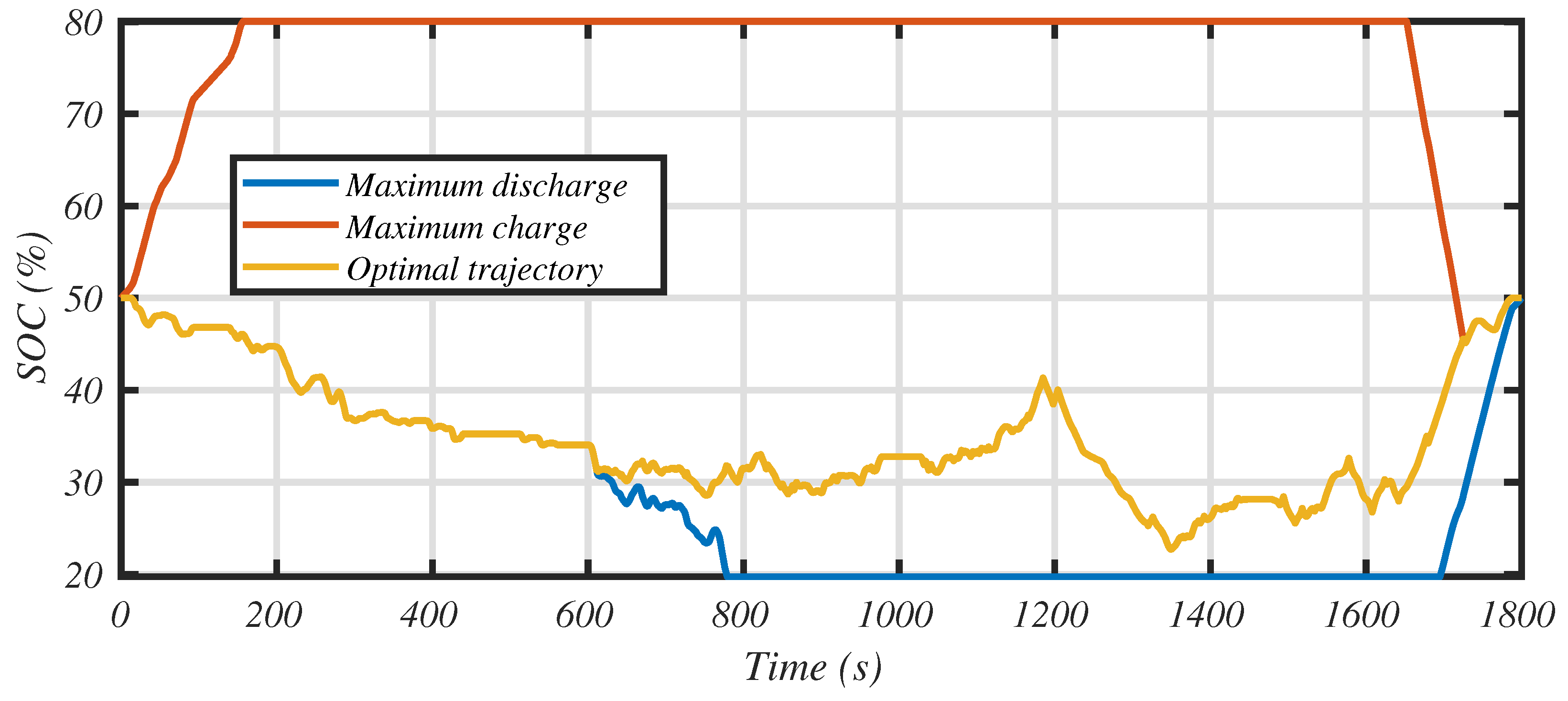
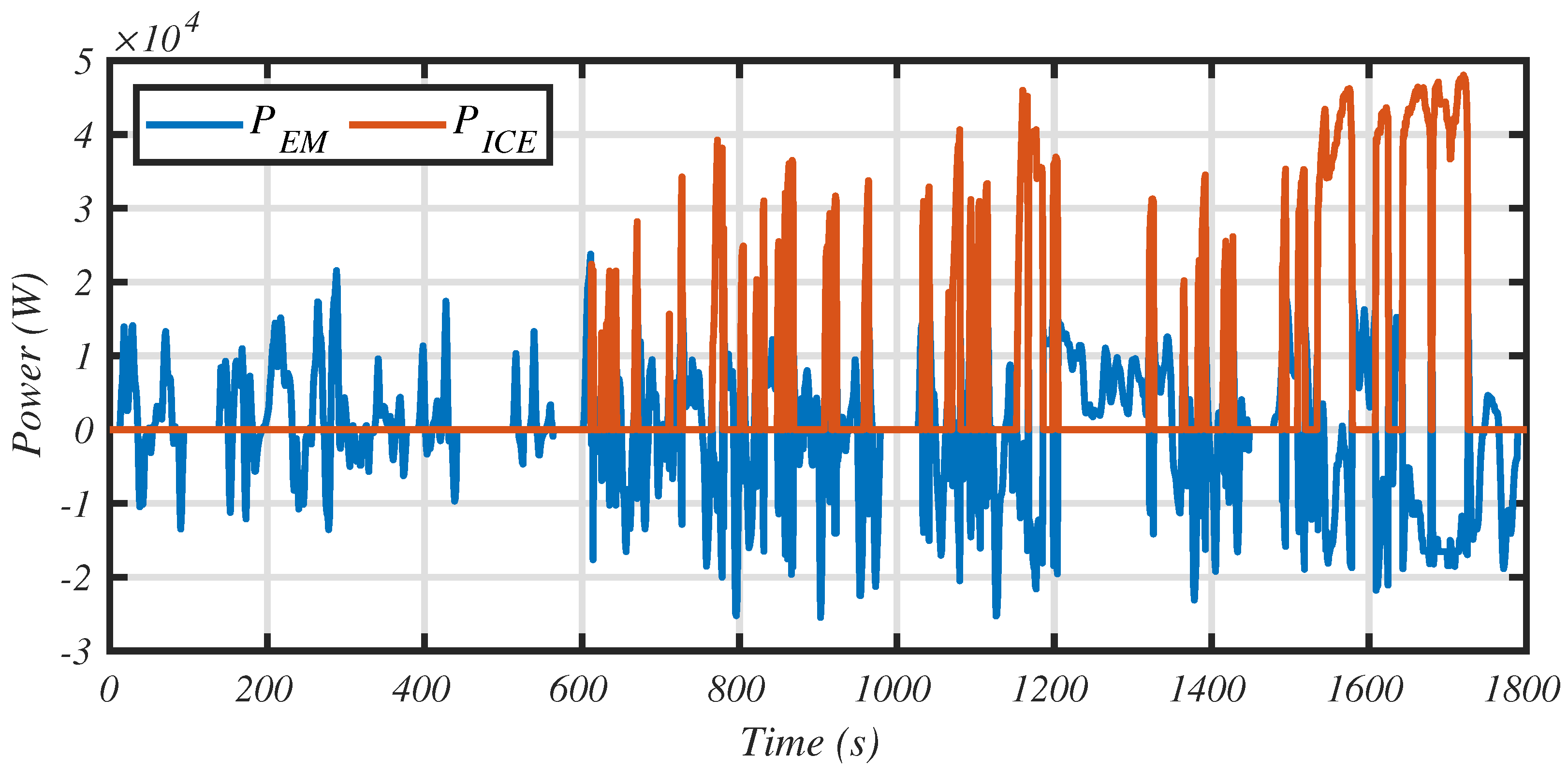
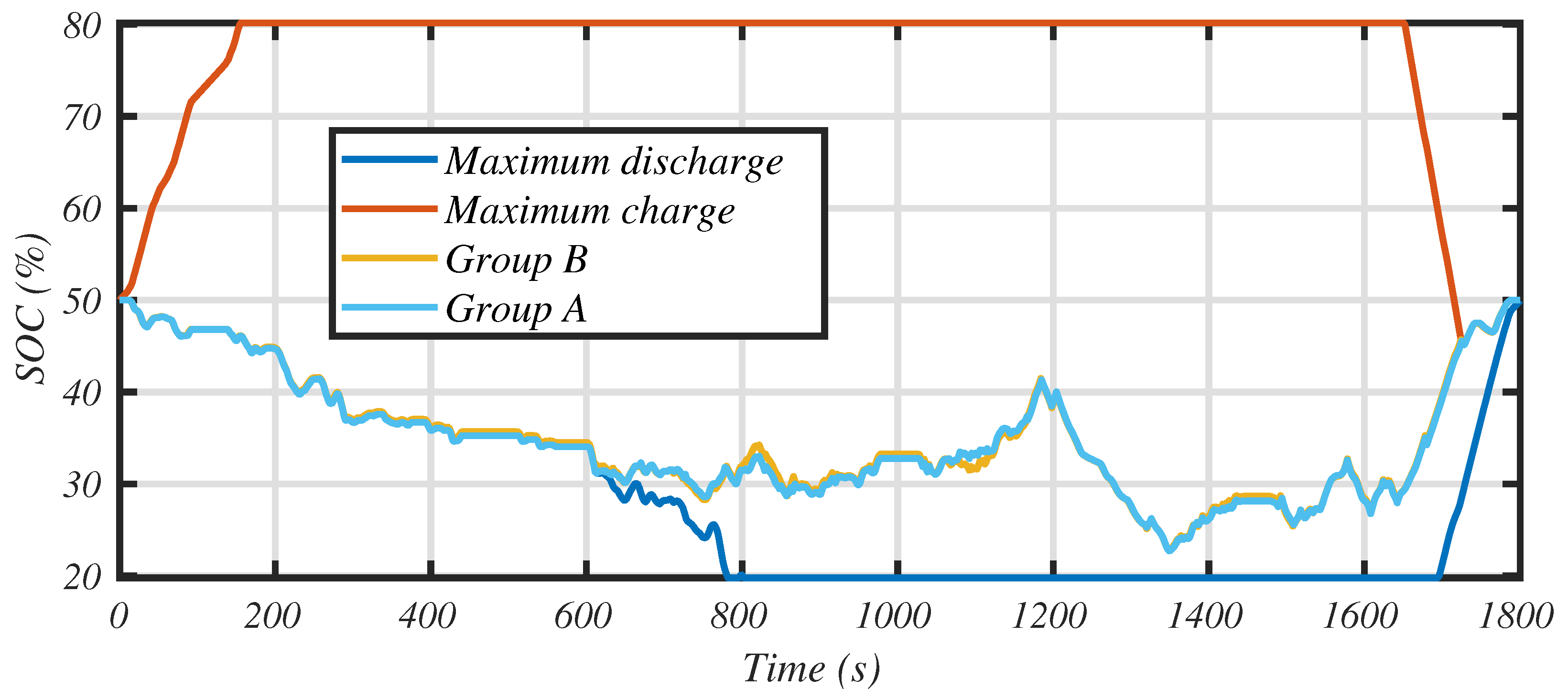
Figure 13 represents the variation of the state of charge of the battery. The lower bound (in blue line) corresponds to the strategy that maximizes the discharge of the battery (i.e., the all-electric mode), while the red curve represents its maximum charge (i.e., the engine is providing maximum power). Of course, because we are simulating a charge sustaining hybrid, the curve must converge at the end of the driving cycle. This surface defines the admissible operating area. The yellow line is the optimal trajectory regarding the objective function. We conclude that the first part of the driving cycle is made in all-electric mode. This is confirmed in Figure 14, where we observe that the urban part is driven with the electric motor alone. We also notice that when the IC engine is started, the electric motor runs in recovery mode, thus recharging the battery. We also observe in Figure 13 that the optimal strategy is not far from the maximum discharge rate. This is only due to the fact that the more aggressive part of the driving cycle happens at the end, which gives the right conditions for the ICE to develop high power and recharge the battery with the best global efficiency (see Figure 14).
Figure 15 shows how the strategy operates regarding the operating points of the ICE and EM. First, we notice that a cloud of points is located near the full load of the ICE, which also matches with the best efficiency area. The blue points denote the operating point used with a cold and thus low efficiency catalyst. Although these points correspond to full open throttle (see intake pressure in Figure 16, plot a), as the spark advance is delayed by 20 to 30 degrees (plot b), the resulting torque is low. During this stage, the strategy increases exhaust enthalpy in order to quickly warm the catalyst. Of course, these operating points present a low thermal efficiency, but this behavior last only a few seconds over the WLTC driving cycle, thus producing a minor impact on global fuel consumption. At the same time, engine admits a lean mixture (air to fuel equivalence ratio lower than 1, see Figure 16, plot c), but as the catalyst is cold, it has no impact on its behavior. This has a small effect, but increases engine efficiency and exhaust temperature while reducing CO emissions at the engine outlet.
As soon as the catalyst is primed, the strategy has to conciliate conflicting constraints:
- For the fuel, the major parameters will be the relative spark advance, which has to be close to its optimal value (). It is also clear that an intake pressure close to atmospheric pressure eliminates pressure drop at the intake valve, thus maximizing efficiency;
- CO is not influenced by the spark advance, but only by the equivalent air to fuel ratio. A low value of is better for CO engine emission. That is not what we observed. Several factors explain this result:
- −
- In this narrow window, CO emissions variation are low;
- −
- CO efficiency is very high when catalyst is primed;
- −
- The strategy greatly reduces CO emission before catalyst light-off (see Figure 10).
- The HC level is very low, and its performance index, is less than 0.1 (see Figure 12), so it has no impact on the control parameters;
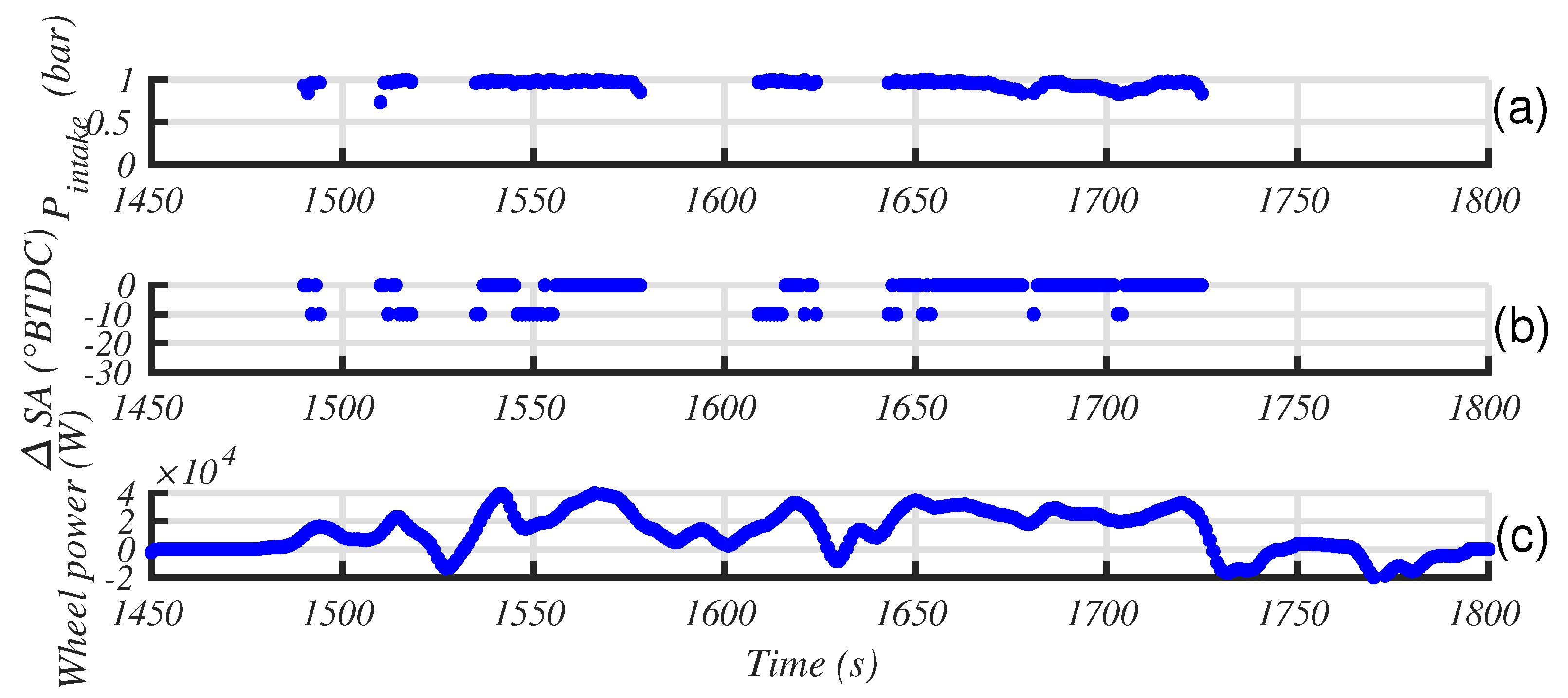
- NOx clearly deeply influences the strategy; we observe a slight enrichment of the mixture ( = 1.008) that drives the catalyst efficiency to 0.995 (see Figure 4). Conversely, we notice an alternation of the relative spark advance between 0 and −10°. This last value means firing later than is optimal, thus reducing the temperature in the combustion chamber and the feedgas NO level. Finally, the temporal distribution of the spark advance values is questionable. It seems to be correlated with the driving power; the strategy adopts a null relative spark advance when the driving power is high, and delays ignition when the wheel power decreases. This interpretation is highlighted in Figure 18.
3.3. Parametric Study on Engine Displacement
We propose in this section to analyze the impact of engine displacement on the performance of the pollution-centered scenario. The displacement varies from 0.8 up to 2.0 L. Accordingly, the engine weight and its inertia vary with the same proportions. The computations are conducted with the Group B parameters values in the WLTC driving cycle (see Table 8). Eight combinations of spark advance and air to fuel equivalence ratio are considered.
One can see on Table 9 that emissions stay relatively stable while the engine displacement varies, but there is a certain gap in fuel consumption; indeed, there is an almost 10% increase in fuel economy between 2.0 and 1.0 L. The variation in global vehicle weight and inertia only explains 3 to 4%. This means that there is an optimal engine size that minimizes whole drive train losses; i.e., it allows the engine to run in its optimal operating range while lowering electric motor and battery losses.
We also compare, for the nominal case (i.e., engine displacement = 1.6 L) the result of the two simulations. Figure 20 shows that the aggregated results are very close and this is the same for temporal behavior, as shown in Figure 21. The last simulation runs eight times faster and consumes almost five times less memory. This is encouraging, as compromises can be found between the two groups of hypotheses.
4. Discussion
We chose to balance each pollutant with the same weighting factor in the objective function. The optimal strategy depends on these values used to scale and weight the emissions. Different compromises can be obtained, but the results presented in this paper show that with a small increase in fuel consumption (less than 3% for NEDC and 5% for WLTC), we observe a reduction of NOx emissions by a factor 20, and thus pass the EU6 regulation limits.
HC emissions are very low, even for the fuel consumption scenario. This is due to the fact that we do not take into account internal cylinder temperature during a cold start. This factor has an effect on the quality of combustion and increases HC emission before that the cylinder’s walls become hot. Moreover, to stabilize combustion during this phase, enrichment occurs, which promotes unburned hydrocarbons. This pollutant is very influenced by the cold start and less influenced by the operating parameters during the whole drive cycle [33]. To take this phenomenon in account, we should add a new state variable simulating the cylinder mean temperature.
Given the verticality of the catalyst efficiency curves, especially the NOx one, a very small change in the equivalence ratio or efficiency S-curve shape can have a significant influence on the results. In practice, it is not possible to control the gas chemistry with such precision in a real engine, especially in the case of transient operations that are common with hybridization. Actual equivalence ratio control strategies usually consist of oscillating around the unit value of equivalence ratio to oxidize CO and HC on the one hand and reduce NO on the other. In addition, the catalyst has oxygen storage capabilities that allow small deviations during transient operations. The model of this equivalence ratio control loop is very complex and involves many state variables, so it is not realistic to take it into account when using dynamic programming.
Regarding the method used in this paper, we wanted to run the code with a step time of 1 s, as it is the necessary condition to limit the rounding errors due to quantization. We used a computer that was equipped with two processors running at 2.2 GHz and with 256 GB of RAM. We tried to limit the use of memory by storing only the variables that were mandatory to solve the graph. The conclusion is that the calculation time is long, resource intensive, and it is difficult to increase the combinatory on the control variables or add more state variables to the models.
Running the code with a step time of 2 s allows the use of natural cooling with a more reasonable temperature grid. Results presented on Section 3.3 are promising, as the same results were observed while using almost five times less computer memory.
5. Conclusions
This study shows how to drive the control parameters of a port fuel injection engine in a hybrid architecture with respect to fuel consumption and pollutant emissions. It gives insight on how to use the degree of freedom represented by spark advance, air to fuel equivalence ratio, and intake pressure. It is known that delaying spark advance allows the early priming of the catalyst. However, our algorithm demonstrates when it should be done and the level of magnitude go bring it to optimality.
To summarize the work, we analyzed the influence of three parameters of close engine control: intake pressure (by the way of SOE), equivalence ratio, and ignition timing:
- Over a wide range of variation, the equivalence ratio acts on the trade-off between the efficiency of the pollution control system and the fuel consumption because the optimal efficiency of the engine is with a lean mixture. However, when emissions are taken into account, the optimal range of variation of the equivalence ratio is reduced by a stoichiometric proportion. In this small range of variation, the equivalence ratio plays a role in the trade-off between the reduction of NO on one hand and of HC and CO on the other. As previously mentioned, a more precise model of the influence of this variable would be necessary to deepen this analysis of equivalence ratio control;
- The optimal strategy degrades the ignition timing to optimize the catalyst priming phase, as in a conventional vehicle. Indeed, despite the reduction in the efficiency of the combustion engine, the ignition delay has a double positive effect on pollution. A significant delay in relation to optimal ignition increases the temperature of the gases at the engine outlet while reducing the concentrations of HC and NO. This ensures that the catalyst is primed as soon as possible while reducing emissions during this critical phase when the catalyst is not yet active. Once the catalyst is primed, the hybrid strategy taking into account pollutant emissions and therefore often tends to delay the advance. This impacts the temperature in the chamber and thus reduces NO emissions;
- The intake pressure is directly linked to the power developed by the internal combustion engine and acts on the one hand on the concentration of NO and HC at the engine outlet and on the other hand on the efficiency of the engine. This latter effect is predominant in the optimal strategy, as the weighted factor for fuel is high in the objective function.
The work is conducted in a backward model environment that allows optimal methods to be deployed. This is a great improvement compared to trial-and-error methods, which are complex and time consuming when the search domain is wide. Dynamic programming is robust and supplies a reference on how to operate an engine in a hybrid vehicle. The drawback of this method is that the dynamic description of the engine has to be quite simple. Other optimization methods can now be explored in light of these results. Additional state variables can be introduced to the models. This work is a milestone that provides us with the opportunity to develop models and to move towards real-time applications.
Author Contributions
Conceptualization, B.J. and A.G.D.B.; methodology, All; software, B.J. and A.G.D.B.; investigation, A.K., A.G.D.B. and B.J.; writing—original draft preparation, B.J.; writing—review and editing, All; supervision, S.P. and L.L.M.; All authors have read and agreed to the published version of the manuscript.
Funding
This research received no external funding.
Conflicts of Interest
The authors declare no conflict of interest.
Abbreviations
The next list describes acronyms and symbols used within the body of the document:
| Acronyms and chemical components | |
| BC | Black Carbon |
| BSFC | Brake Specific Fuel Consumption in g/kWh |
| BTDC | Before Top Dead Center |
| CAD | Crank Angle Degree |
| CO | Carbon Monoxide |
| CPU | Central Processing Unit |
| DP | Dynamic Programming |
| ECU | Engine Control Unit |
| EM | Electric Machine |
| HC | Unburned Hydrocarbons |
| ICE | Internal Combustion Engine |
| NEDC | New European Driving Cycle |
| NO | Nitrogen Oxide |
| NOx | Nitrogen Oxides |
| PM | Particulate Matter |
| PMP | Pontryaguin Maximum Principle |
| RAM | Random Access Memory |
| SA | Spark Advance |
| TWC | Three Way Catalyst |
| WLTC | Worldwide harmonized Light-duty vehicles Test Cycle |
| Symbols used in the equations | |
| [CO] | CO concentration in ppm |
| [HC] | HC concentration in ppm |
| [NO] | NO concentration in ppm |
| [NO] | Saturation value for [NO model] |
| Weighting factor expressing the relative influence of consumption versus CO emissions | |
| Weighting factor expressing the relative influence of consumption versus HC emissions | |
| Weighting factor expressing the relative influence of consumption versus NO emissions | |
| Relative spark advance in CAD BTDC | |
| Discretization step for the time in s | |
| Air to fuel equivalence ratio (/) | |
| Adjusting parameters for the [CO model] | |
| Adjusting parameters for the [HC model] | |
| Reference fuel mass flow in g·s−1 | |
| Fuel mass flow in g·s−1 | |
| Reference mass flow of pollutant species X in g·s−1 | |
| Mass flow of pollutant species X in g·s−1 | |
| Adjusting parameters for the [NO model] | |
| Intake pressure in bar | |
| Spark advance (CAD BTDC) | |
| Battery state of charge in % | |
| Battery state of energy in J | |
Appendix A. Algorithm Overview
The core of the algorithm was developed with MATLAB® and comprises three main parts:
- Constructing the graph: this consists of calculating at each time step the cost-to-go function represented by all the feasible commands that satisfy the constraints of the system. This is the costliest part (in term of CPU and RAM), as all paths between the two time steps have to be calculated in term of SOC and temperature, fuel, emissions, and finally cost-to-go function. The size of certain variables depends on the states and the size others depend on the commands. Finally, they are classified using a unique identifier denoted hereafter:A minimization is done at this stage; several commands lead to a particular node in the graph, specified by a value of . For each node, the command that minimizes the cost-to-go function must be found (see below). This is the place in the algorithm dealing with the largest number of variables. It initially uses MATLAB’s sortrows function. As explained in the help function:[B,I] = sortrows(A,…) also returns an index vector I, which describes the order of the sorted rows, namely, B = A(I,:).By making a vector A of size (n, 2) with the identifier in the first column and the cost-to-go function in the second column, one can ordinate the identifier in B and the corresponding indices in I. At this step, it is easy to get the indices of the minimal cost in the original vectors. The job is done, but the drawback with this function is that the element of Matrix A must be of the same type, i.e., double precision floating numbers (for input arguments and output arguments also). This uses a large amount of memory. By developing our own C-sfunction in MATLAB with a fast top-down implementation of a merge-sort algorithm, we created our own prototype, thus enabling an identifier of type uint32, such as this one (freeing a lot of memory):[id_in_order(uint32), order_cost(uint32)] = csortrows(id(uint32), cost(double))
- Storing the variables: to solve the graph (third part of the algorithm), the vector of the optimal commands()has to be stored at each time step along with the previous nodes to know where they come from.
- Finding the optimal path: the optimal path is characterized by the minimal cost-to-go function at the end of the driving cycle that satisfies the SOC constraints. Obtaining this index allows one, starting from the end and going backwards step by step up to the beginning of the cycle, to know the optimal commands and the preceding node. Once this is done, all intermediate variables can be recalculated.
References
- Crippa, M.; Oreggioni, G.; Guizzardi, D.; Muntean, M.; Schaaf, E.; Lo Vullo, E.; Solazzo, E.; Monforti-Ferrario, F.; Olivier, J.; Vignati, E. Fossil CO2 and GHG Emissions of All World Countries: 2020 report; Publications Office of the European Union: Luxembourg, 2020. [Google Scholar] [CrossRef]
- Vincent, C.; Peyaud, V.; Laarman, O.; Six, D.; Gilbert, A.; Gillet-Chaulet, F.; Berthier, É.; Morin, S.; Verfaillie, D.; Rabatel, A.; et al. Déclin des deux plus grands glaciers des Alpes françaises au cours du XXIe siècle: Argentière et Mer de Glace. La Météorol. 2019, 1, 49. [Google Scholar] [CrossRef]
- European Environment Agency. Emissions of Air Pollutants from Transport; Technical Report; European Environment Agency: Kobenhavn, Denmark, 2019. [Google Scholar]
- European Environment Agency. Air Pollution; Technical Report; European Environment Agency: Kobenhavn, Denmark, 2020. [Google Scholar]
- CITEPA. Gaz à Effet de Serre et Polluants Atmosphériques—Bilan des Emissions en France de 1990 à 2017; Rapport National d’Inventaire: Paris, France, 2019. [Google Scholar]
- Kalghatgi, G. Is it really the end of internal combustion engines and petroleum in transport? Appl. Energy 2018, 225, 965–974. [Google Scholar] [CrossRef]
- Helmers, E.; Dietz, J.; Weiss, M. Sensitivity Analysis in the Life-Cycle Assessment of Electric vs. Combustion Engine Cars under Approximate Real-World Conditions. Sustainability 2020, 12, 1241. [Google Scholar] [CrossRef] [Green Version]
- IEA. Global Energy Review 2020; Technical Report; IEA: Paris, France, 2020. [Google Scholar]
- Masson-Delmotte, V.; Zhai, P.; Pirani, A.; Connors, S.; Péan, C.; Berger, S.; Caud, N.; Chen, Y.; Goldfarb, L.; Gomis, M.; et al. Climate Change 2021: The Physical Science Basis. Contribution of Working Group I to the Sixth Assessment Report of the Intergovernmental Panel on Climate Change; Cambridge University Press: Cambridge, UK, 2021. [Google Scholar]
- Leach, F.; Kalghatgi, G.; Stone, R.; Miles, P. The scope for improving the efficiency and environmental impact of internal combustion engines. Transp. Eng. 2020, 1, 100005. [Google Scholar] [CrossRef]
- International Council on Clean Transportation. Too Low to Be True? How to Measure Fuel Consumption and CO2 Emissions of Plug-in Hybrid Vehicles, Today and in the Future; The National Academies of Sciences, Engineering, and Medicine: Washington, DC, USA, 2017. [Google Scholar]
- Mensing, F.; Bideaux, E.; Trigui, R.; Ribet, J.; Jeanneret, B. Eco-driving: An economic or ecologic driving style? Transp. Res. Part C 2014, 38, 110–121. [Google Scholar] [CrossRef]
- Pandey, V.; Jeanneret, B.; Gillet, S.; Keromnes, A.; Le Moyne, L. A simplified thermal model for the three way catalytic converter. In Proceedings of the TAP 2016, 21st International Transport and Air Pollution Conference, Lyon, France, 24–26 May 2016; p. 6. [Google Scholar]
- Brandt, E.; Wang, Y.; Grizzle, J.W. Dynamic modeling of a three-Way catalyst for SI engine Exhaust emission control. IEEE Trans. Control. Syst. Technol. 2000, 8, 767–776. [Google Scholar] [CrossRef]
- Brandt, E.P.; Grizzle, J.W. Three-way catalyst diagnostics for advanced emissions control systems. In Proceedings of the 2001 American Control Conference (Cat. No.01CH37148), Arlington, VA, USA, 25–27 June 2001; Volume 5, pp. 3305–3311. [Google Scholar] [CrossRef]
- Shaw, B.T.; Fisher, G.D.; Hedrick, J.K. A simplified coldstart catalyst thermal model to reduce hydrocarbon emissions. IFAC 2002, 35, 312. [Google Scholar] [CrossRef] [Green Version]
- Hedinger, R.; Elbert, P.; Onder, C. Optimal Cold-Start Control of a Gasoline Engine. Energies 2017, 10, 1548. [Google Scholar] [CrossRef] [Green Version]
- Yusuf, A.A.; Inambao, F.L. Effect of cold start emissions from gasoline-fueled engines of light-duty vehicles at low and high ambient temperatures: Recent trends. Case Stud. Therm. Eng. 2019, 14, 100417. [Google Scholar] [CrossRef]
- Fontaras, G.; Pistikopoulos, P.; Samaras, Z. Experimental evaluation of hybrid vehicle fuel economy and pollutant emissions over real-world simulation driving cycles. Atmos. Environ. 2008, 42, 4023–4035. [Google Scholar] [CrossRef]
- Guille des Buttes, A. Optimisation Conjointe de la Consommation d’Essence et des Emissions de Polluants Réglementés pour un Véhicule Hybride Essence-Electrique d’Architecture Parallèle. PhD Thesis, École Doctorale ED160 EEA, Lyon, France, 2021. [Google Scholar]
- Zhang, P.; Yan, F.; Du, C. A comprehensive analysis of energy management strategies for hybrid electric vehicles based on bibliometrics. Renew. Sustain. Energy Rev. 2015, 48, 88–104. [Google Scholar] [CrossRef]
- Saerens, B.; Diehl, M.; Bulck, E. Optimal Control Using Pontryagin’s Maximum Principle and Dynamic Programming; Springer: London, UK, 2010. [Google Scholar]
- Guille des Buttes, A.; Jeanneret, B.; Kéromnès, A.; Le Moyne, L.; Pélissier, S. Energy management strategy to reduce pollutant emissions during the catalyst light-off of parallel hybrid vehicles. Appl. Energy 2020, 266, 114866. [Google Scholar] [CrossRef]
- Jeanneret, B.; Guille Des Buttes, A.; Pelluet, J.; Keromnes, A.; Pélissier, S.; Le Moyne, L. Optimal Control of a Spark Ignition Engine Including Cold Start Operations for Consumption/Emissions Compromises. Appl. Sci. 2021, 11, 971. [Google Scholar] [CrossRef]
- European Commission. Regulation (EU) 2019/631; Technical Report; European Commission: Luxembourg, 2020. [Google Scholar]
- Bellman, R. Dynamic Programming; Dover Books on Computer Science Series; Dover Publications: New York, NY, USA, 2003. [Google Scholar]
- Sundstrom, O.; Guzzella, L. A generic dynamic programming Matlab function. In Proceedings of the 2009 IEEE Control Applications, (CCA) Intelligent Control, (ISIC), St. Petersburg, Russia, 8–10 July 2009; pp. 1625–1630. [Google Scholar] [CrossRef]
- Elbert, P.; Ebbesen, S.; Guzzella, L. Implementation of Dynamic Programming for n-Dimensional Optimal Control Problems with Final State Constraints. IEEE Trans. Control. Syst. Technol. 2013, 21, 924–931. [Google Scholar] [CrossRef]
- Guzzella, L.; Onder, C.H. Introduction to Modeling and Control of Internal Combustion Engine Systems; Springer: Berlin/Heidelberg, Germany, 2010. [Google Scholar] [CrossRef]
- Vinot, E.; Scordia, J.; Trigui, R.; Jeanneret, B.; Badin, F. Model simulation, validation and case study of the 2004 THS of Toyota Prius. Int. J. Veh. Syst. Model. Test. 2008, 3, 139–167. [Google Scholar] [CrossRef]
- Ngo, V.; Hofman, T.; Steinbuch, M.; Serrarens, A. Effect of Gear Shift and Engine Start Losses on Control Strategies for Hybrid Electric Vehicles. World Electr. Veh. J. 2012, 5, 125–136. [Google Scholar] [CrossRef] [Green Version]
- Ngo, V.D.; Navarrete, J.A.C.; Hofman, T.; Steinbuch, M.; Serrarens, A. Optimal gear shift strategies for fuel economy and driveability. Proc. Inst. Mech. Eng. Part D J. Automob. Eng. 2013, 227, 1398–1413. [Google Scholar] [CrossRef]
- Cedrone, K.; Cheng, W. SI engine control in the cold-fast-idle period for low HC emissions and fast catalyst light off. SAE Int. J. Engines 2014, 7, 968–976. [Google Scholar] [CrossRef] [Green Version]
Figure 1.
Parallel hybrid architecture corresponding to the reference vehicle.

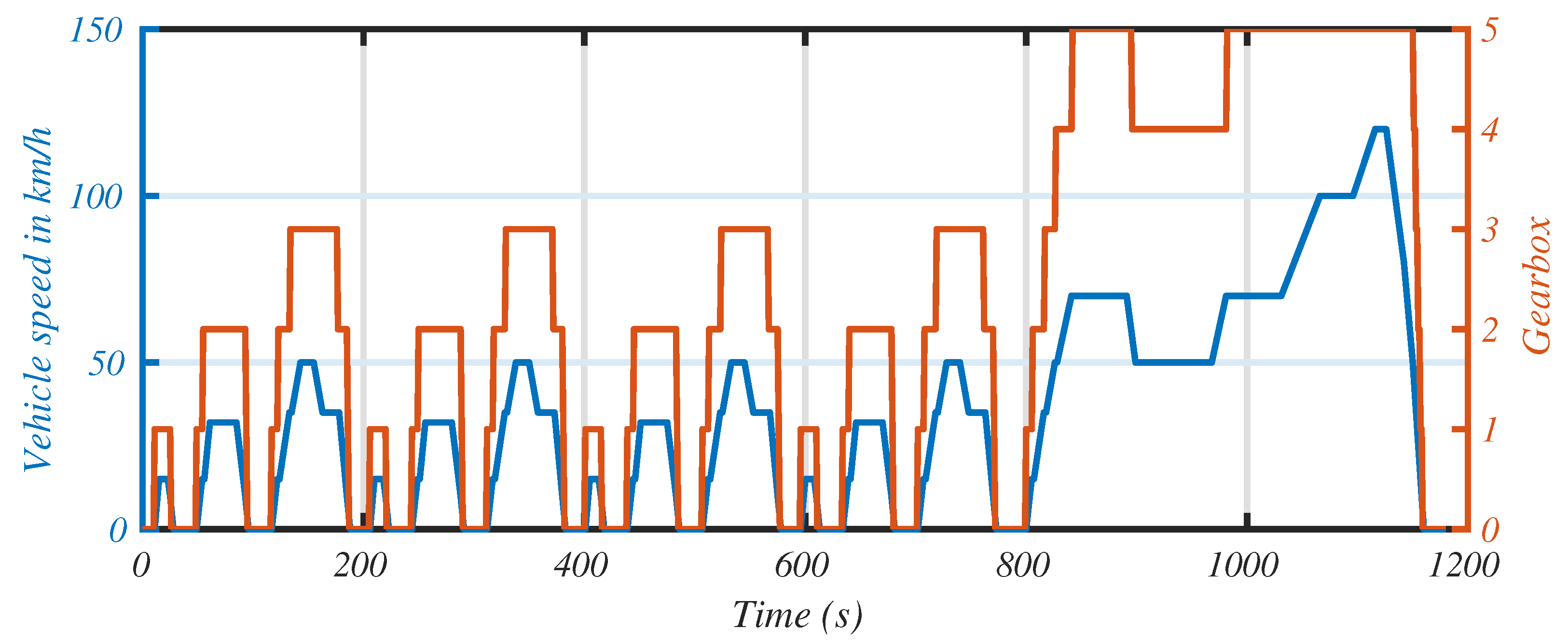
Figure 2.
Speed profile and gearbox ratios for the NEDC driving cycle.

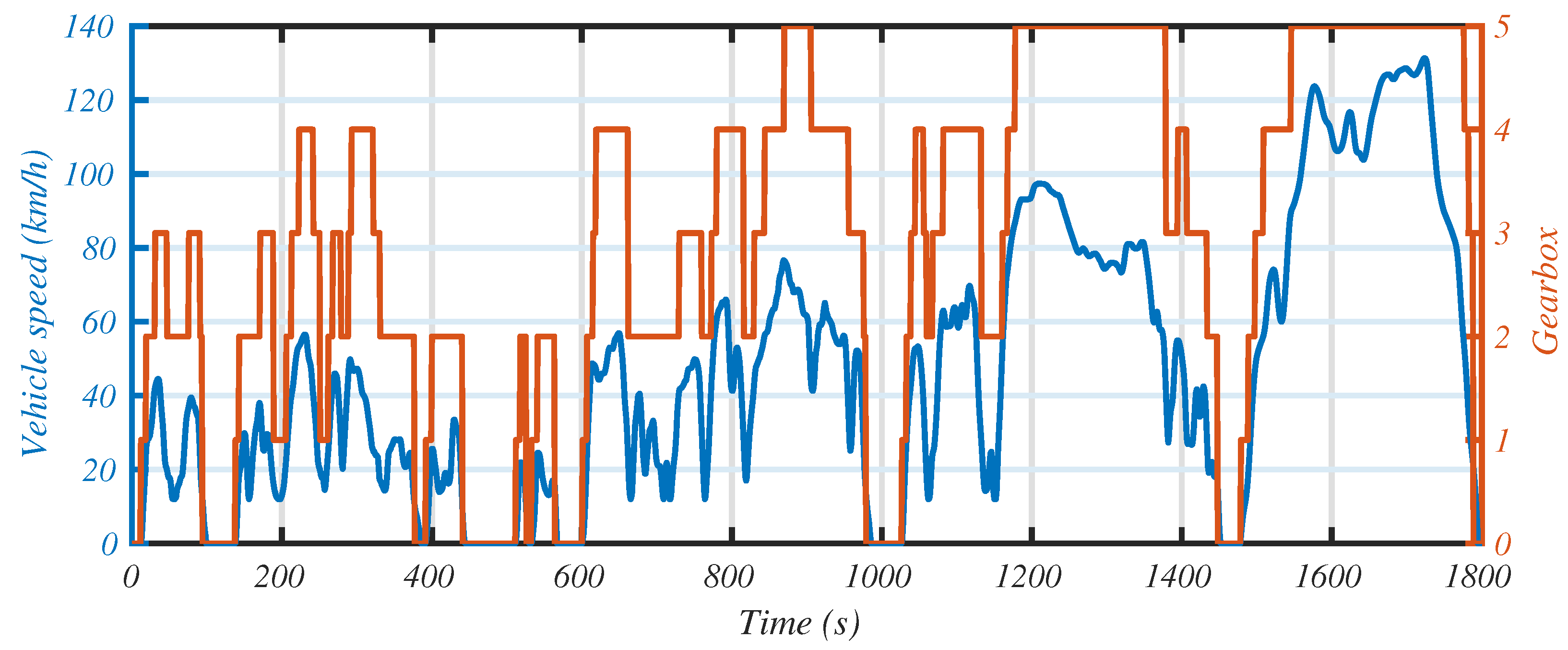
Figure 3.
Speed profile and gearbox ratios for the Class 3 WLTC driving cycle.

Figure 4.
Catalyst conversion efficiency model (a): regarding air to fuel equivalence ratio; (b): function of catalyst temperature.
Figure 4.
Catalyst conversion efficiency model (a): regarding air to fuel equivalence ratio; (b): function of catalyst temperature.

Figure 5.
Emission model at 2000 rpm; 0.9 Bar; relative spark advance varies from −20° to 20°.

Figure 6.
(a): Internal combustion engine map; (b): electric motor map.

Figure 7.
Catalyst temperature evolution.

Figure 8.
Natural cooling try (a): Temperature evolution; (b): Temperature gradient.

Figure 9.
Operating points for consumption-centered strategy in the WLTC driving cycle. (red squares mean that the catalyst temperature is higher than the light-off temperature; blue squares mean that it is lower). (a): engine; (b): electric motor.
Figure 9.
Operating points for consumption-centered strategy in the WLTC driving cycle. (red squares mean that the catalyst temperature is higher than the light-off temperature; blue squares mean that it is lower). (a): engine; (b): electric motor.

Figure 10.
Cumulative emissions for consumption-centered strategy in the WLTC driving cycle. (a): Carbon monoxyde; (b): unburned Hydrocarbons; (c): Nytrogen oxides.
Figure 10.
Cumulative emissions for consumption-centered strategy in the WLTC driving cycle. (a): Carbon monoxyde; (b): unburned Hydrocarbons; (c): Nytrogen oxides.

Figure 11.
Temperature evolution and catalyst efficiency for the consumption-centered strategy in the WLTC driving cycle.
Figure 11.
Temperature evolution and catalyst efficiency for the consumption-centered strategy in the WLTC driving cycle.

Figure 12.
Comparison of the performance index in the WLTC driving cycle.

Figure 13.
SOC trajectory with the emission-centered strategy in the WLTC driving cycle.

Figure 14.
Power sharing with the emission-centered strategy in the WLTC driving cycle.

Figure 15.
Operating points for the emission-centered strategy in the WLTC driving cycle. (red squares mean that the catalyst temperature is higher than the light-off temperature; blue squares mean that it is lower). (a): engine; (b): electric motor.
Figure 15.
Operating points for the emission-centered strategy in the WLTC driving cycle. (red squares mean that the catalyst temperature is higher than the light-off temperature; blue squares mean that it is lower). (a): engine; (b): electric motor.

Figure 16.
Control parameters with the emission-centered strategy in the WLTC driving cycle. (a): intake pressure; (b): relative spark advance; (c): air to fuel equivalence ratio.
Figure 16.
Control parameters with the emission-centered strategy in the WLTC driving cycle. (a): intake pressure; (b): relative spark advance; (c): air to fuel equivalence ratio.

Figure 17.
Pollutant emissions with the emission-centered strategy in the WLTC driving cycle. (a): Carbon monoxyde; (b): unburned Hydrocarbons; (c): Nytrogen oxides.
Figure 17.
Pollutant emissions with the emission-centered strategy in the WLTC driving cycle. (a): Carbon monoxyde; (b): unburned Hydrocarbons; (c): Nytrogen oxides.

Figure 18.
Correlation between relative spark advance and wheel power (zoom during the highway part of the WLTC driving cycle). (a): intake pressure; (b): relative spark advance; (c): wheel power.
Figure 18.
Correlation between relative spark advance and wheel power (zoom during the highway part of the WLTC driving cycle). (a): intake pressure; (b): relative spark advance; (c): wheel power.

Figure 19.
Results of the parametric study.

Figure 20.
Comparison of the performance index between Group A and Group B discretization in the WLTC driving cycle.
Figure 20.
Comparison of the performance index between Group A and Group B discretization in the WLTC driving cycle.

Figure 21.
SOC profile evolution between Group A and Group B discretization in the WLTC driving cycle.
Figure 21.
SOC profile evolution between Group A and Group B discretization in the WLTC driving cycle.


Table 1.
Main vehicle characteristics (Chassis Peugeot 308 SW—Model/Year 2009) and models used in this study.
Table 1.
Main vehicle characteristics (Chassis Peugeot 308 SW—Model/Year 2009) and models used in this study.
| Component | Size | Type of Model |
|---|---|---|
| IDI gasoline engine | 1.6 L | Mean value engine model |
| Three-way catalytic converter | EURO 6 compliant | 0D model |
| PRIUS II type electric motor | resized to 25 kW | Quasistatic map |
| (mechanical power) | ||
| Kokam Li-ion Battery | 31 kW–1.7 kWh | Voltage source and resistance |
| Gear box 20DP42 | 5 gears | Constant efficiency |
| Vehicle weight | 1504 kg | Longitudinal forces |
Table 2.
EURO6 and CAFE regulations.
| Fuel Cons. | CO2 | CO | HC | NOx |
|---|---|---|---|---|
| l/100 km | g/km | g/km | g/km | g/km |
| 4.0 | 95 | 1.0 | 0.1 | 0.060 |
Table 3.
Parametric study on battery energy step over the WLTC cycle (100 J is the reference).
| Fuel Cons. | CO | HC | NOx | Form Factor | |
|---|---|---|---|---|---|
| J | l/100 km (%) | g/km | g/km | g/km | |
| 100 | 4.392 (0.0) | 0,131 | 0.009 | 0.165 | 1.0 |
| 500 | 4.393 (0.03) | 0.133 | 0.009 | 0.167 | 0.997 |
| 750 | 4.395 (0.06) | 0.133 | 0.009 | 0.167 | 0.996 |
| 1500 | 4.398 (0.13) | 0.133 | 0.009 | 0.167 | 0.993 |
| 3000 | 4.403 (0.26) | 0.132 | 0.009 | 0.166 | 0.987 |
| 5000 | 4.416 (0.54) | 0.137 | 0.010 | 0.165 | 0.978 |
Table 4.
Variation of the traction energy over the WLTC cycle as a function of the time step (10 Hz reference).
Table 4.
Variation of the traction energy over the WLTC cycle as a function of the time step (10 Hz reference).
| Step Time (s) | ||||
|---|---|---|---|---|
| Traction Energy (Wh/km) | 135.9 | 135.2 | 133.0 | 124.7 |
| Variation (%) | Reference | −0.5 | −2.2 | −8.2 |
Table 5.
Performance of the consumption centered scenario.
| Optim. | Driving | Fuel Cons. | CO2 | CO | HC | NOx |
|---|---|---|---|---|---|---|
| Parameter | Cycle | l/100 km | g/km | g/km | g/km | g/km |
| Group A | NEDC | 3.58 | 84 | 0.213 | 0.014 | 0.171 |
| Group A | WLTC | 4.40 | 103 | 0.133 | 0.009 | 0.167 |
Table 6.
Discretization step size used in this section.
| Variable | Steps | Min. Value | Max. Value |
|---|---|---|---|
| Optimization parameter | Group A | not applicable | |
| Equivalence ratio | 0.005 | 0.993 | 1.008 |
| Relative spark advance | 10° | −30° | 0° |
| Step time | 1 s | not applicable | |
Table 7.
Performance of the emission-centered scenario.
| Drive | Fuel Cons. | CO2 | CO | HC | NOx | RAM | Calc. |
|---|---|---|---|---|---|---|---|
| Cycle | l/100 km | g/km | g/km | g/km | g/km | Gb | Time (h) |
| NEDC | 3.77 | 89 | 0.302 | 0.007 | 0.009 | 133 | 57 |
| WLTC | 4.52 | 106 | 0.306 | 0.007 | 0.008 | 155 | 95 |
Table 8.
Discretization step size used in the parametric study.
| Variable | Steps | Min. Value | Max. Value |
|---|---|---|---|
| Optimization parameters | Group B | not applicable | |
| Fuel/air eq. ratio | 0.15 | 0.993 | 1.008 |
| Relative spark advance | 10° | −30° | 0° |
| Step time | 2 s | not applicable | |
Table 9.
Results of the parameter study.
| Engine | Fuel Cons. | CO2 | CO | HC | NOx | RAM | Calc. |
|---|---|---|---|---|---|---|---|
| Displ. | l/100 km | g/km | g/km | g/km | g/km | Gb | Time (h) |
| 0.8 | 4.26 | 100 | 0.291 | 0.007 | 0.011 | 19 | 5 |
| 1.0 | 4.26 | 100 | 0.294 | 0.006 | 0.008 | 22 | 7 |
| 1.2 | 4.29 | 101 | 0.299 | 0.007 | 0.009 | (Results not available) | 9 |
| 1.4 | 4.38 | 103 | 0.298 | 0.006 | 0.008 | (Results not available) | 10 |
| 1.6 | 4.48 | 105 | 0.304 | 0.006 | 0.008 | 34 | 12 |
| 1.8 | 4.57 | 108 | 0.312 | 0.007 | 0.008 | 40 | 12 |
| 2.0 | 4.69 | 110 | 0.319 | 0.007 | 0.008 | 40 | 13 |
Publisher’s Note: MDPI stays neutral with regard to jurisdictional claims in published maps and institutional affiliations. |
© 2022 by the authors. Licensee MDPI, Basel, Switzerland. This article is an open access article distributed under the terms and conditions of the Creative Commons Attribution (CC BY) license (https://creativecommons.org/licenses/by/4.0/).
Share and Cite
MDPI and ACS Style
Jeanneret, B.; Guille Des Buttes, A.; Keromnes, A.; Pélissier, S.; Le Moyne, L. Optimal Control for Cleaner Hybrid Vehicles: A Backward Approach. Appl. Sci. 2022, 12, 578. https://0-doi-org.brum.beds.ac.uk/10.3390/app12020578
AMA Style
Jeanneret B, Guille Des Buttes A, Keromnes A, Pélissier S, Le Moyne L. Optimal Control for Cleaner Hybrid Vehicles: A Backward Approach. Applied Sciences. 2022; 12(2):578. https://0-doi-org.brum.beds.ac.uk/10.3390/app12020578
Chicago/Turabian StyleJeanneret, Bruno, Alice Guille Des Buttes, Alan Keromnes, Serge Pélissier, and Luis Le Moyne. 2022. "Optimal Control for Cleaner Hybrid Vehicles: A Backward Approach" Applied Sciences 12, no. 2: 578. https://0-doi-org.brum.beds.ac.uk/10.3390/app12020578
Note that from the first issue of 2016, this journal uses article numbers instead of page numbers. See further details here.