
Research on Initial Model Construction of Seismic Inversion Based on Velocity Spectrum and Siamese Network

School of Geophysics and Information Technology, China University of Geosciences, Beijing 100083, China
*
Author to whom correspondence should be addressed.
Appl. Sci. 2022, 12(20), 10593; https://0-doi-org.brum.beds.ac.uk/10.3390/app122010593
Submission received: 31 August 2022
/
Revised: 19 October 2022
/
Accepted: 19 October 2022
/
Published: 20 October 2022
(This article belongs to the Special Issue Technological Advances in Seismic Data Processing and Imaging)
Abstract
:The initial model plays an important role in seismic inversion. Generally, the initial model is constructed by lateral extrapolation of parameters under horizons constraints. However, without horizon data, initial modeling becomes a challenging task. Velocity spectrum is a 2D image that can reflect the characteristics of the formations. We regard the problem of establishing the initial model as the problem of similarity analysis of seismic lateral characteristics and propose a method of establishing the initial inversion model based on velocity spectrum and Siamese network. Firstly, the lateral variation of formation characteristics is tracked on velocity spectra generated by common depth point (CDP) gathers. Then, the target tracking results at different CDP positions are obtained with the triple Siamese network. Finally, the discrete inversion parameters are extrapolated along the tracking paths to obtain the initial inversion model. The Siamese network can quickly obtain the similarity of 2D images and does not need manual labels. The theoretical and practical results show that our method can efficiently generate the initial model that conforms to the seismic structure and stratigraphic characteristics without the constraint of interpreted horizon data.
1. Introduction
Establishing the initial model is one of the necessary and key steps of the model-based inversion method, which has a great impact on the inversion effect. Traditionally, the method of generating the initial model is to extrapolate the inversion parameters observed from the wells or vertical seismic profile (VSP) along the interfaces picked from seismic profiles [1,2] or to extrapolate the seismic attributes [3,4,5,6,7]. In these methods, seismic horizons are necessary and manual interpretations are required. Horizon picking is one of the most time-consuming and labor-intensive steps [8]. Automatic horizon interpretation technology has been developing. Many geophysicists have proposed a variety of algorithms to improve the efficiency and accuracy of automatic horizons tracking [9,10,11,12,13,14], but these methods still need some prior information, such as manually setting up seed points or carrying out manual interpretation of large sets of strata. It is difficult to establish the initial model directly without manual interpretation. In addition, seismic inversion usually requires the initial model to cover the entire 3D region, but in practice, the automatic interpretation of the entire data volume is difficult to achieve. Therefore, there is a need for an efficient and accurate seismic extrapolation method to establish an initial model with the condition of lack of horizons.
Neidall et al. [15] presented the concept of velocity spectrum. The seismic gathers are automatically scanned with equal velocity intervals, and the velocity spectra are generated by stacking energy or similarity coefficient. Compared with artificial horizon interpretation, the velocity spectra are easier to generate. In conventional seismic data processing, stacking or migration velocity is obtained by velocity analysis on velocity spectra. The hyperbolas in the prestack seismic gathers reflect the characteristics of the interfaces, and the velocity spectrum contains the position and velocity information of each hyperbola in prestack gathers. Compared with the gathers, the features on velocity spectrum are more focused. The velocity spectrum is a 2D image, which can be used to identify the changes of the lateral characteristics of the formation.
Deep learning technology has shown much better performance than traditional neural network methods in speech and visual tasks, such as image classification [16], semantic segmentation [17], and image segmentation [18]. This is mainly due to the strong feature expression ability of deep networks such as convolutional neural network (CNN). In the field of exploration geophysics, deep learning has been successfully applied to seismic processing and interpretation [19,20]. However, most of the current applications need to manually make and label samples first, and then extract the corresponding type of feature information from the seismic images. For the establishment of the initial inversion model, it is still unable to get rid of the dependence on horizons. Deep learning has the potential to provide more global information. As an important part of computer vision, visual target tracking technology has been developed rapidly. The Siamese network uses the idea of similarity learning, describes the tracking problem as an object matching problem, and judges the position of objects by comparing the similarity of objects [21,22].
In this paper, we transformed the parameter extrapolation problem in constructing the initial inversion model into a 2D image tracking problem and proposed a method for constructing the initial model based on velocity spectrum and Siamese network. Firstly, the velocity spectra generated by CDP gathers were used to track the lateral variation of formation characteristics. Then, the target tracking results at different CDP positions were obtained by combining the similarity of the triple Siamese network analog velocity spectrum. Finally, the discrete inversion parameters were extrapolated along the tracking path to obtain the initial model. We proposed an improved triple Siamese structure, which adds an update branch to solve the lateral variation of velocity spectrum characteristics during target tracking. This improvement takes dynamic update into tracking. In order to verify the applicability of the method, we carried out tests on theoretical and practical data. The results show that it can automatically obtain the extrapolation paths and can be used to establish the initial model of seismic inversion.
2. Materials and Methods
2.1. Velocity Spectrum
The velocity spectrum [15] is a 2D image generated by scanning and stacking (or correlating) energy along different velocities on each CDP gather using the similarity criterion. The x and y axes are the velocity and two-way travel time, respectively. The velocity spectrum is composed of a series of energy clusters, and the velocity information is determined according to the abscissa position of the energy clusters. Most of the current research on velocity spectrum focuses on improving the resolution of velocity spectrum and then improving the accuracy of velocity pickup [23,24,25,26,27,28,29]. The application of deep learning in velocity analysis almost focuses on the automatic pickup of energy clusters in velocity spectrum [30,31,32].
In addition to the position and velocity information that can be used for velocity analysis in conventional seismic processing, velocity spectrum is also a 2D image that can reflect formation characteristics. Velocity spectra also have advantages in identifying lateral characteristics of formation. The reasons are as follows: firstly, the interference of complex underground structures and noise always leads to incomplete, staggered, and amplitude varying hyperbolas, while the velocity spectrum scans and superimposes the events along the hyperbola, which can attenuate the non-hyperbolic noise to a certain extent. Secondly, in most cases, the energy clusters in velocity spectrum corresponds to the interfaces. Because the formation interfaces have relatively coherent structure in the underground space, the velocity spectra of adjacent CDP points have similarity, and the characteristics of the formation interface can be obtained from the velocity spectra by this similarity. The velocity spectrum Formula (1) is as follows:
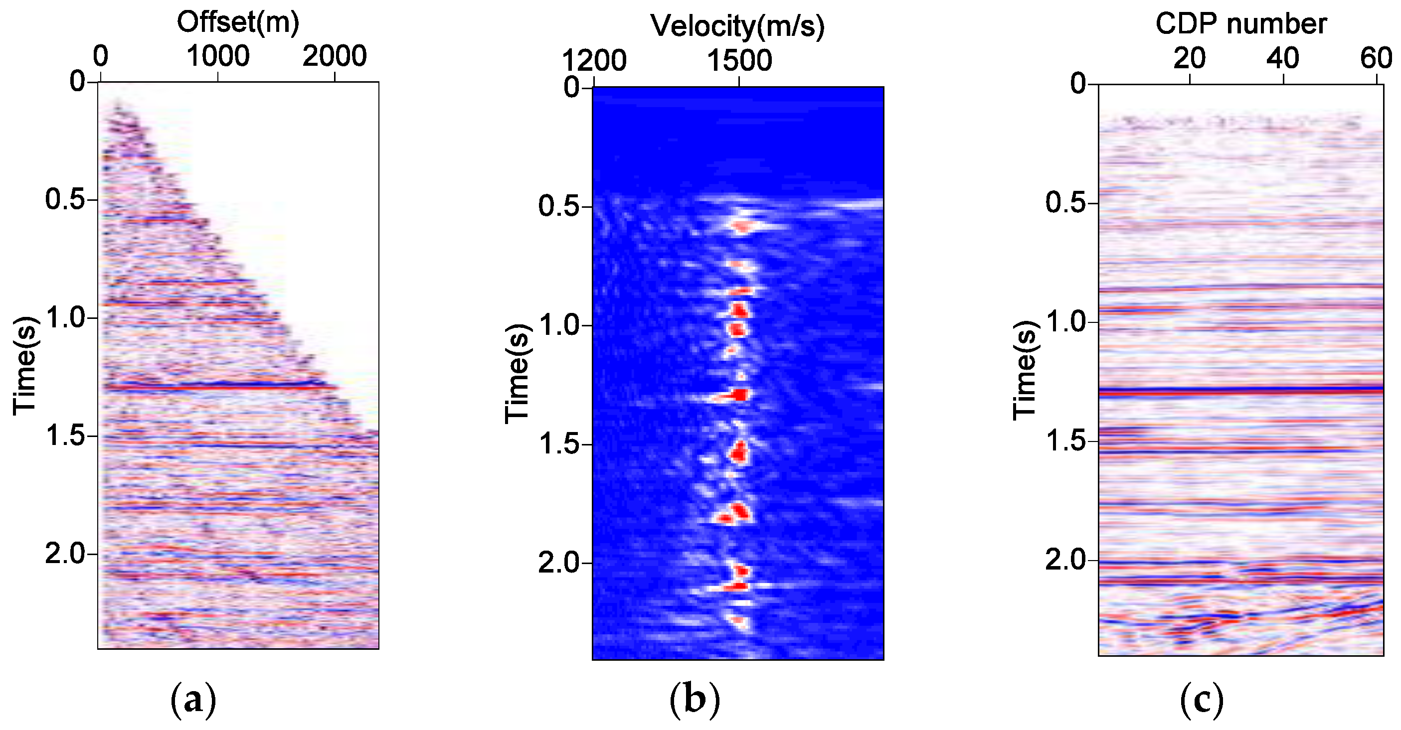
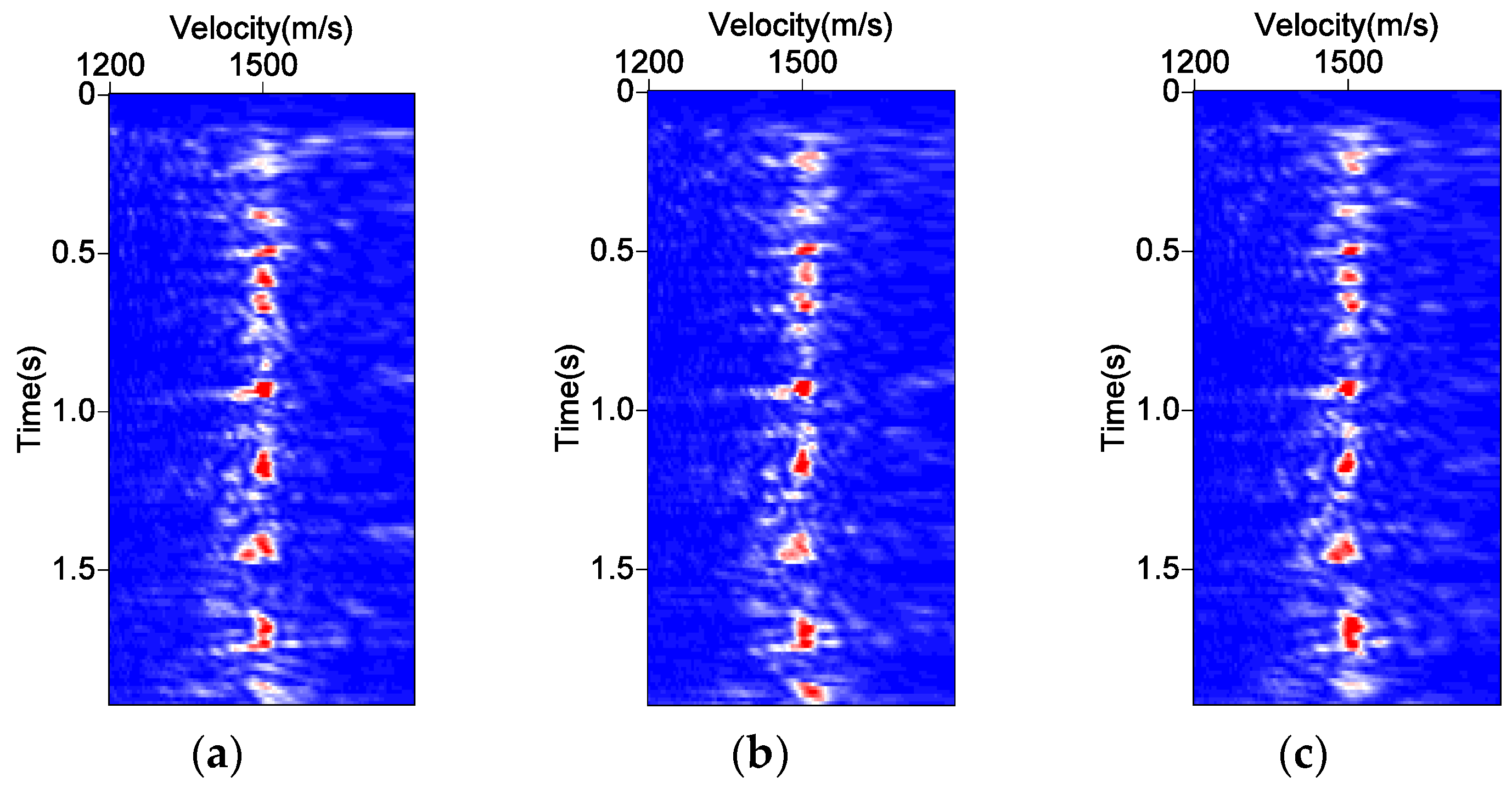
where M is the length of the time window, N is the offset length, I is the number of seismic traces in the CDP gather, and is the amplitude at offset i and time j. According to Formula (1), if all seismic traces are the same, S equals to 1. If each seismic trace is a random value, S approaches 0. Only when the scanning velocity is equal to the normal move-out (NMO) velocity, the waveforms of each trace are the most similar, in-phase stacking is realized within the time window, and S is close to 1. Here, we use real seismic data after conventional data processing and prestack migration to show the consistency between energy clusters in velocity spectrum and formation interfaces. Figure 1a is the common reflection point (CRP) gather at the location of CDP number 30 (CDP 30), which has undergone NMO removal processing with v = 1500 m/s. Figure 1b is the velocity spectrum generated from the gather shown in Figure 1a. The x and y axes are the velocity and two-way travel time, respectively. The center of the energy clusters in velocity spectrum corresponds to the maximum value of stacking energy. Figure 1c is the stack section. It can be seen that the centers of the energy clusters correspond to the events on the seismic section. Each energy cluster corresponds to an obvious formation interface. Figure 2a–c are velocity spectra of CDP 32, CDP 34, and CDP 36, respectively. The three velocity spectra have high similarity. With the similarity of the energy clusters in lateral, the positions of the formation interfaces can be obtained by tracking the energy clusters.
2.2. The Triple Structure Siamese Network for Velocity Spectra Lateral Target Tracking
For lateral target tracking in velocity spectra, the prior materials are the images of the energy clusters in the given windows. The tracking algorithm needs to overcome the challenges of target deformation, background interference, scale change, and angle rotation, and also needs to take into account the accuracy and efficiency. The Siamese network can find a set of parameters, so that the similarity of input images is large when they belong to the same category and small when they belong to different categories. Another advantage of the Siamese network is that the input is a pair of images rather than an image, so it can naturally increase the amount of training data and make full use of limited datasets to train, which is very important in the field of target tracking. In this paper, we improved the traditional Siamese network structure by adding an input update branch. A triple structure Siamese network for velocity spectra lateral target tracking is presented. We set the target area as a positive sample, and the background area and other morphological energy clusters as negative samples. Firstly, the tracking algorithm extracts the features of the target through a series of convolution operations and trains the classifier. Next, the well-trained classifier is used to find the most similar region in the velocity spectra of different CDP positions. Finally, the lateral extrapolation path of inversion parameters can be obtained through the change trend of the target positions. The added update branch can take the prediction result of the current position as an input and update the initial target according to the current tracking result, so as to adapt to the lateral change of the velocity spectrum.
2.2.1. Triple Siamese Network Structure
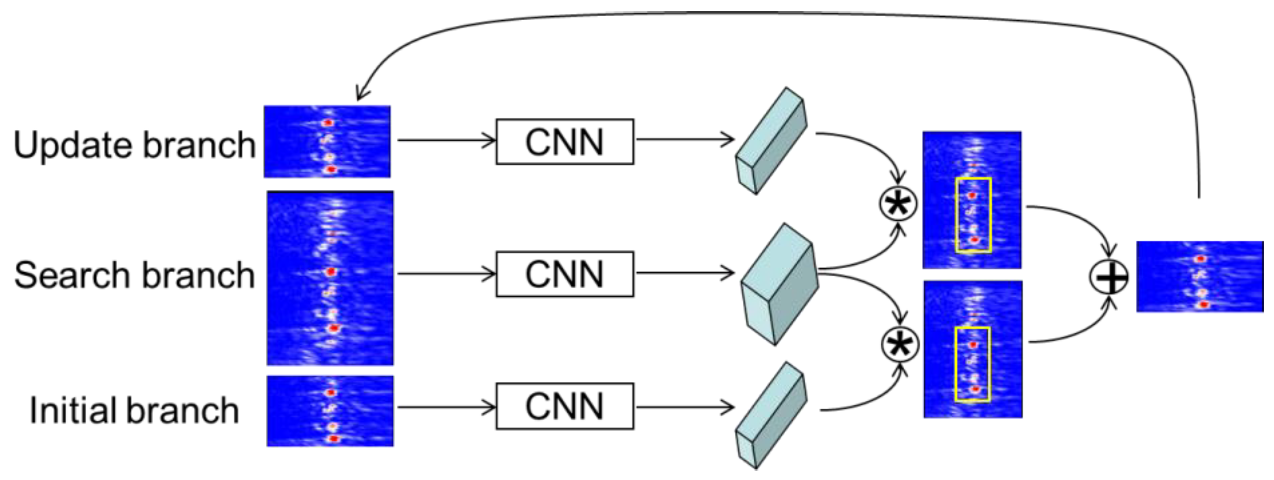
The traditional Siamese network always uses the initial image as the tracking target. However, the velocity spectrum varies in the lateral direction. With the deepening of the tracking process, the information contained in the initial sample is insufficient to track the subsequent targets. We solve this problem by adding an update of target features in the tracker. The velocity spectrum samples at the initial position provide the most basic characteristics of the target and play a leading role in the tracking process. With the lateral movement of the target position, tracking by fusing the previous position features is better than using only the initial samples. Based on this consideration, we proposed a triple structure Siamese network based on the traditional Siamese network. We added an update branch of the current target and used the current prediction result as the target to track the velocity spectrum of the next position. During the tracking process, the current target will be updated with the result of target tracking. The structure of the triple velocity spectrum tracking network is shown in Figure 3.
Different from the traditional Siamese network, the triple network consists of three branches: an initial branch I with an initial target as an input, a search branch S with a search area as an input, and an update branch U with a tracking result at the previous location as an input. The backbone models in the three branches share the same CNN architecture. Through the same network model, the responses of I, S, and U are , , and , which are embedded into the feature space of subsequent tasks. I is the initial branch, and the specified initial velocity spectrum is used as the sample. I remains unchanged throughout the tracking process. U is the update branch, that is, the previous target tracking result. U will be updated with the tracking process. In order to embed the information of these branches, we use the feature map of the updated branch and the feature map of the search area to perform cross-correlation operations. Similar to the traditional Siamese network, the triple network uses a full convolution network for feature extraction, and each channel also generates a corresponding mapping response R. Since there are three branches, the mapping results of two channels are generated, which are:
where ∗ represents a cross-correlation operation. R1 is the mapping result of the initial branch and the search branch, and R2 is the mapping result of the update branch and the search branch. In order to use the two-mapping information, the mapping results are fused weighted :
where and are the weight coefficients, and .
2.2.2. Weight Coefficients
The weight coefficient is determined by the similarity between the current target image and the previously saved image. Here, we use a perceptual Hash algorithm to judge the similarity [33]. We know that the high-frequency information in an image can provide details, and the low-frequency information can describe the frame. Hash algorithm is a method to detect the similarity between images with the low-frequency information of images. First, the image is down-sampled to 8 × 8 to remove high-frequency information and discard the difference caused by different sizes. Next, the image is converted into a gray-scale image, and its gray-scale average value is calculated. Further, the gray value of each pixel in the image is compared with the average gray value. If the gray value is greater than or equal to the average value, it is recorded as 1, and if the gray value is less than the average value, it is recorded as 0. Finally, these 64 values are combined to form the Hash fingerprint of this image. This method is fast and efficient and is not affected by image size or scale. The main process of determining the weight coefficient with Hash algorithm is as follows:
Step 1: calculate the Hash fingerprint of the initial target image and each predicted image.
Step 2: calculate the number Num of different points of the Hash fingerprint between the target image and the predicted image.
Step 3: determine the weight coefficients and according to the value of Num. There are several situations. If Num < 5, the current target is considered to be similar to the initial target image, replace the initial target with the current target, and set = 0, = 1. If 5 < Num < 10, perform image fusion and set = 0.5, = 0.5. If Num > 10, there is a large difference between the current target and the initial target image, the current image is discarded and set = 1, = 0, that is, the initial target image will not be updated. The reasonable threshold (5 and 10 or other number) can be determined by manual test.
2.2.3. Loss Function and Network Parameters
In the mapping result, the points within the search area are positive samples, and the points outside the area are negative samples. The loss function for each point in the mapping result is:
where s is the true value of the point, x is the label of the point, and x∈{+1, −1}. The overall loss of the mapping result is the average of the losses of all points, that is:
where z is the position, x(z) is expressed as:
where h is the step size of the network, c is the center point, and R is the radius of the search area.
The weight coefficients of the similarity discriminant function are solved by the gradient descent method to minimize the error between the sample labels x and the similarity discriminant function. The specific parameters of the network are shown in Table 1. The maximum pooling layer is used after the first two convolution layers, respectively. The Relu nonlinear activation function is used after each convolution layer except the last layer. The batch normalization (BN) layer is embedded after each linear layer. There is no padding in the network.
2.3. Workflow
After the initial target image on the velocity spectrum is given, all subsequent images are compared with the initial target image for similarity. The Siamese network performs full convolution on the search image. In order to find the position of the target in the searched image, all possible positions can be tested exhaustively, and the image with the greatest similarity to the target can be determined. The triple Siamese structure actually calculates the cross-correlation between the two input branches and the search branch, determines the weight coefficient of the branch fusion according to the similarity of the image, and adapts to the lateral change of the velocity spectrum by updating the initial target. The main implementation steps of the method are as follows:
Step 1: generate velocity spectrum images of all positions.
Step 2: extract the target image feature at the specified position and within the specified window by using the initial branch.
Step 3: extract the image feature of the search area at the current position by using the search branch.
Step 4: calculate the cross-correlation between the features and to obtain the target response .
Step 5: extract the target image feature at the specified position and within the specified window by using the update branch.
Step 6: calculate the cross-correlation between the features and to obtain the target response , and take as the current position tracking result.
Step 7: determine the fusion weight coefficients and , and obtain as the new input of the update branch.
Step 8: move the window, repeat steps 3–7 until the velocity spectrum of this position is traversed, and then end the current position task.
Step 9: move the position, repeat steps 2–8 until the velocity spectra of all positions are traversed, and then the whole task is completed.
3. Model Test
In order to verify the feasibility of the method, we carried out tests on theoretical model data and real seismic data. The lateral extrapolation path of inversion parameters is obtained by tracing the lateral position of velocity spectrum according to the method in this paper. In our tests, the interval velocity is used as the inversion parameter to check the extrapolation result. The tests were carried out on a PC equipped with Intel (R) i7 12,700 CPU, an RTX3060TI GPU, 16 GB RAM, and Ubuntu 19 operating system.
3.1. Theoretical Model
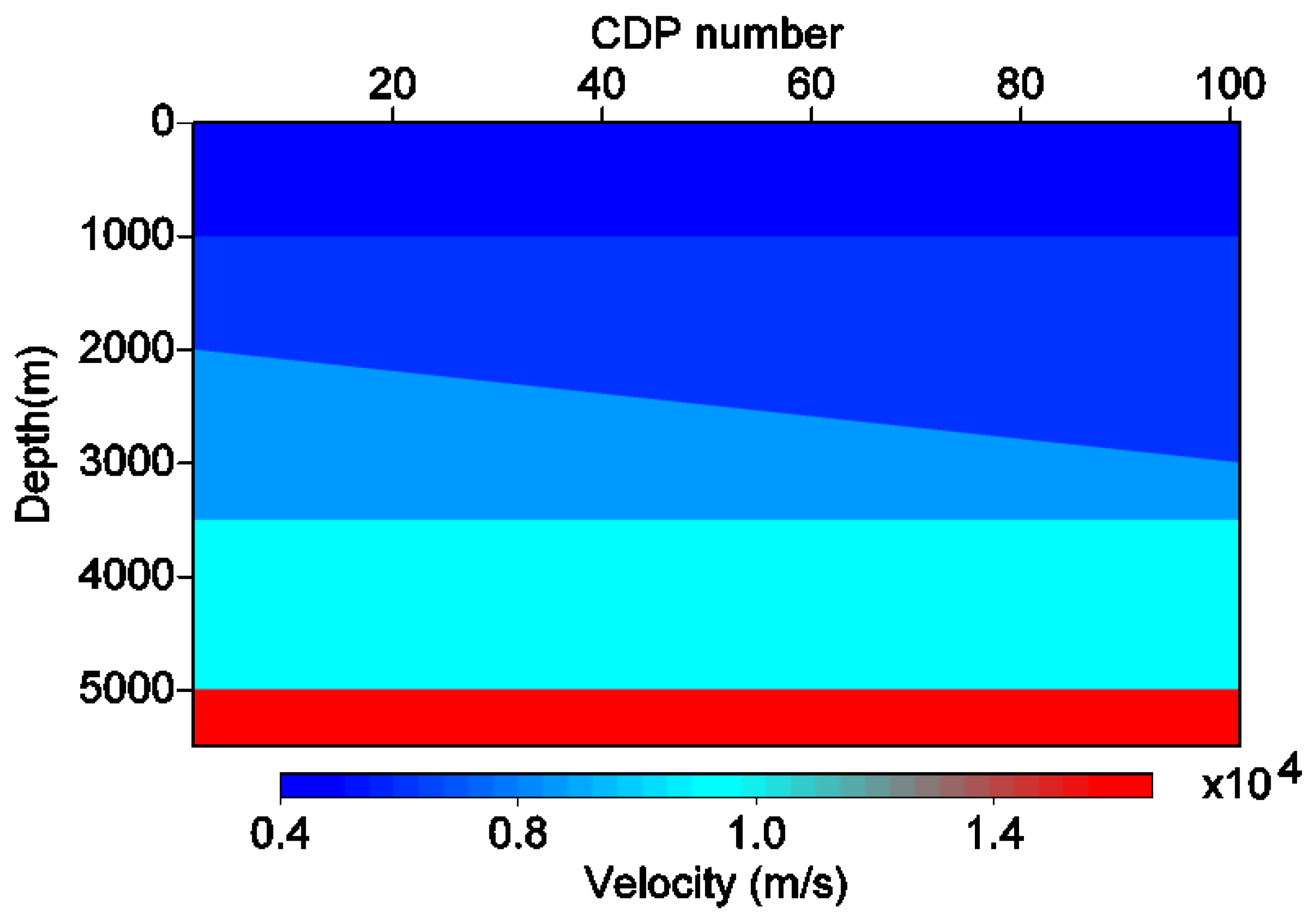
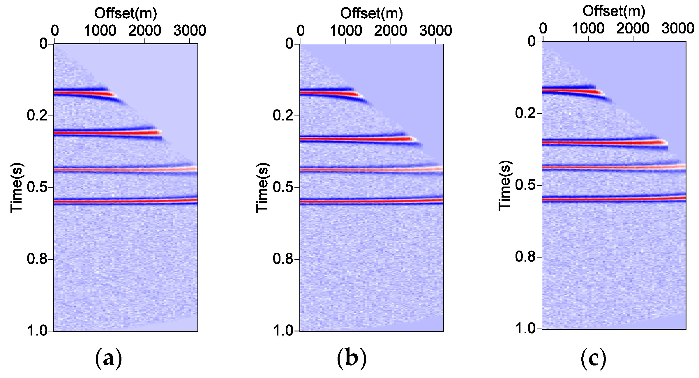
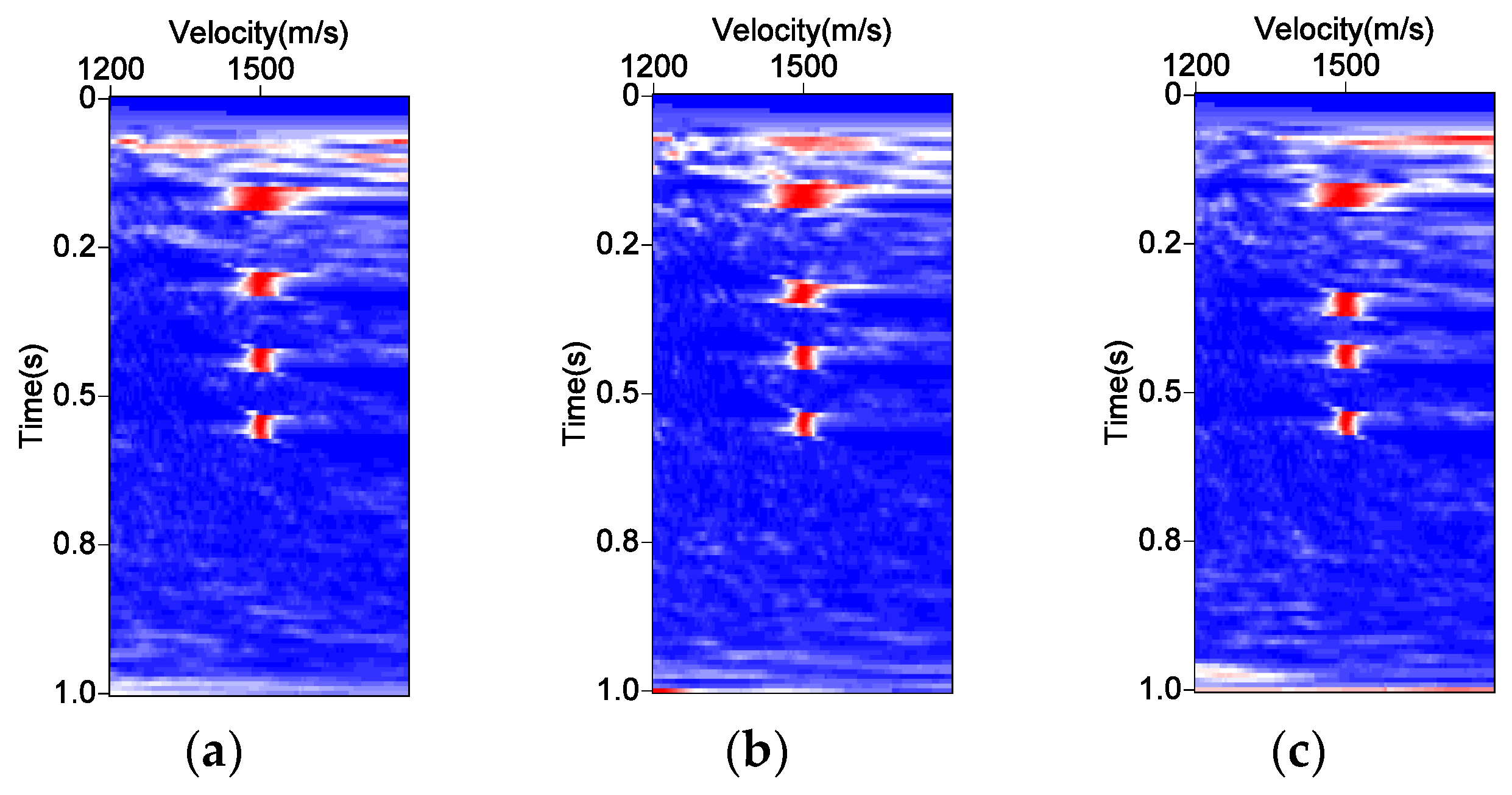
A theoretical model with four interfaces is designed to synthesize seismic data and test the method. The depth of the model is 5500 m and the sampling interval is 5 m. The width of the model is 1000 m, and 100 CDP points are set. The theoretical model of interval velocity is shown in Figure 4. CDP gathers are obtained through forward modeling, with the time length of 1 s and the maximum offset of 3100 m. Figure 5a–c are the CDP gathers at positions of CDP 30, CDP 50, and CDP 70, respectively. For each CDP gather, NMO removal processing is performed according to the root mean square velocity of 1500 m/s and a velocity spectrum is generated. Figure 6a–c are the velocity spectra of CDP 30, CDP 50, and CDP 70, respectively.
3.2. Model Training
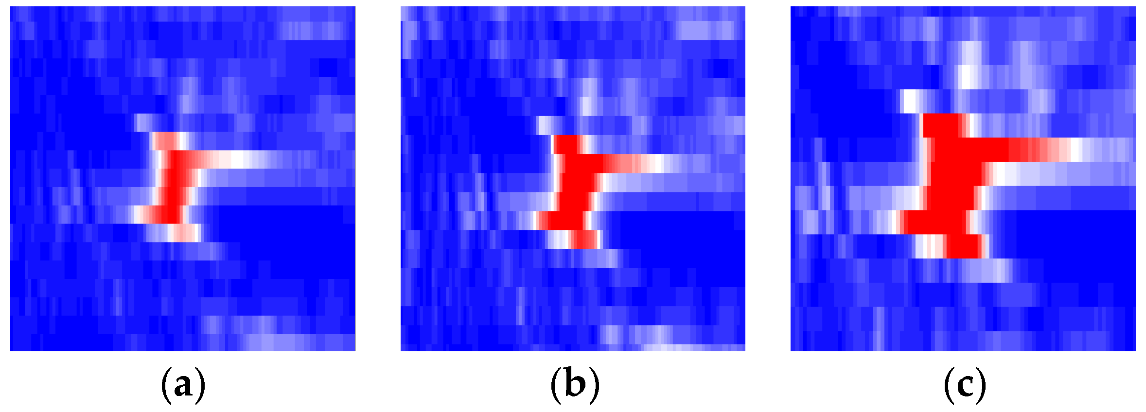
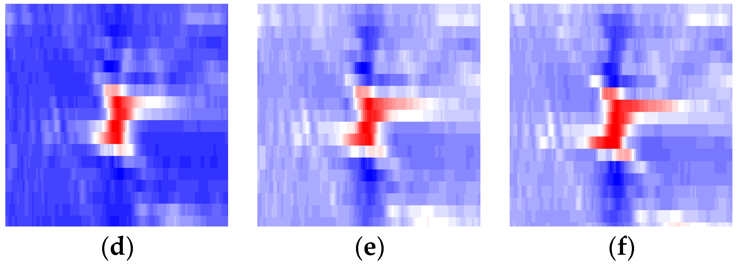
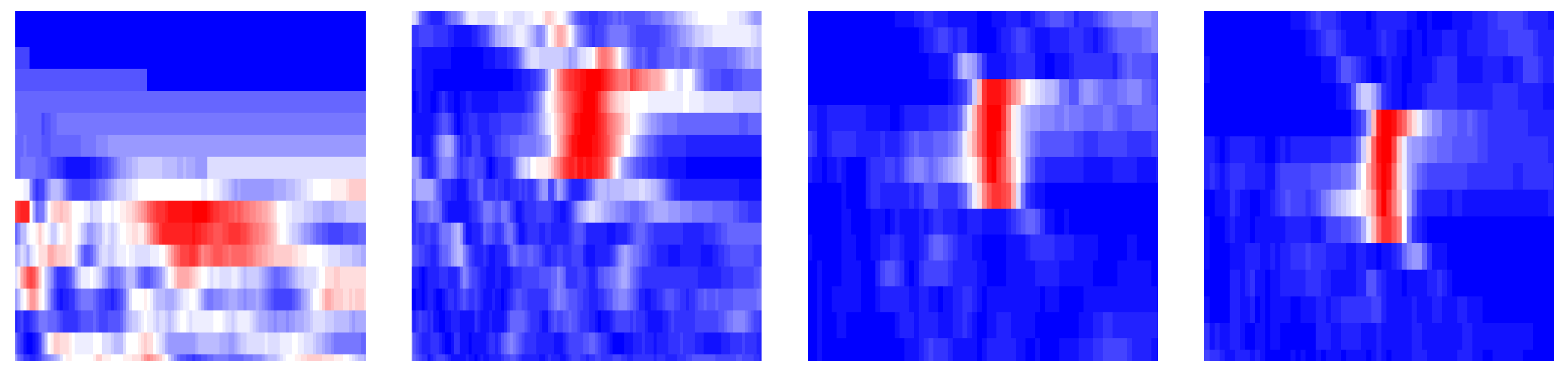
The velocity spectrum of CDP 50 is used as the tracking target of the training dataset. As shown in Figure 6b, there are four energy clusters. We take the energy cluster of 0.2–0.35 s (as shown in Figure 7a) as an example to explain the generation of a training dataset. Based on the energy cluster of 0.2–0.35 s, 100 training samples labeled as positive are generated by stretching, compression, and filtering. Figure 7b,c are examples of images after deformation and stretching, and Figure 7d–f are examples of images after filtering. The positive samples are set to 1.
The energy clusters of 0.1–0.2 s, 0.35–0.5 s, and 0.5–0.65 s in Figure 6b are stretched, compressed, and filtered to generate 300 training samples marked as negative, as shown in Figure 8. The negative samples are set to 0. The training process has 500 iterations, and the learning rate is set to 0.0001. After this training process is completed, set the tracking target as the energy cluster of 0.35–0.5 s, and set the energy clusters of 0.1–0.2 s, 0.2–0.35 s, and 0.5–0.65 s as the negative samples, and then repeat the same training process.
3.3. Tracking Results
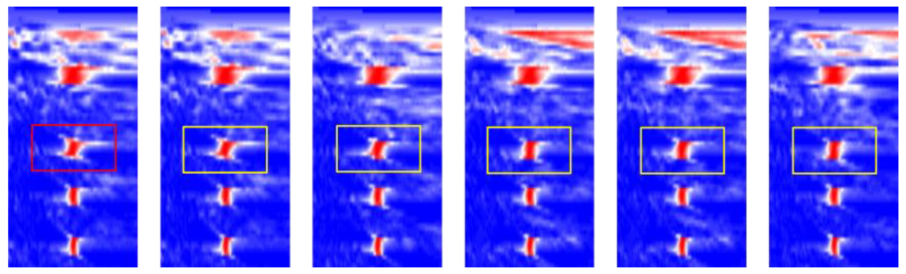
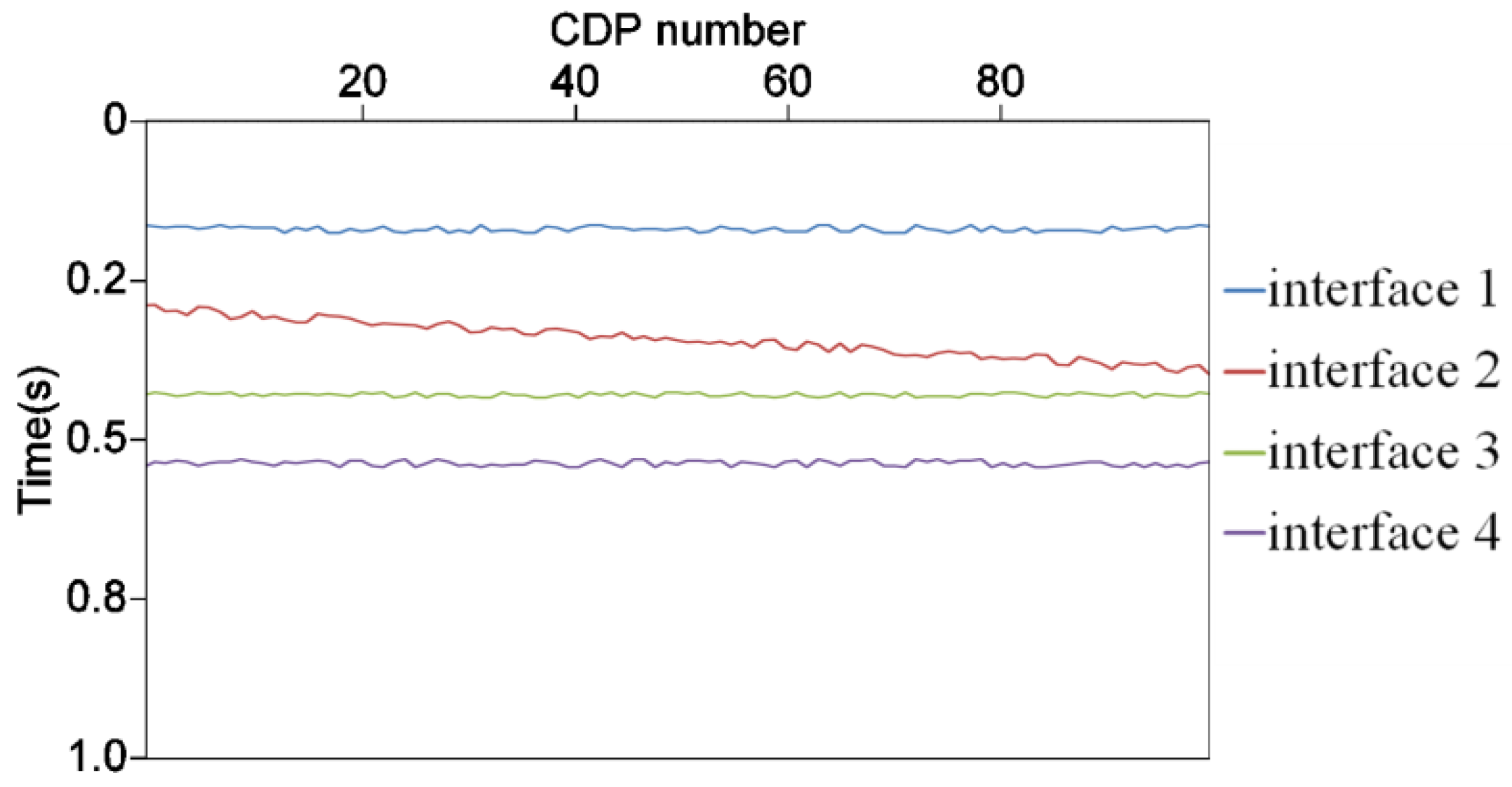
The velocity spectrum images of all 100 CDP points are sequentially tracked. The tracking results of CDP 50 to CDP 55 are shown in Figure 9. The red rectangle is the tracking target, and the yellow rectangle is the velocity spectrum tracking results of different CDPs. The tracking path is formed by connecting the midpoint positions of the tracking results. As shown in Figure 10, the four color lines are the paths of the energy clusters to track laterally. It can be found by comparing Figure 4 that the four tracking paths are consistent with the four interfaces in the model. By extrapolating seismic parameters along the tracking path, the initial model conforming to the underground structure can be obtained.
3.4. Initial Velocity Model
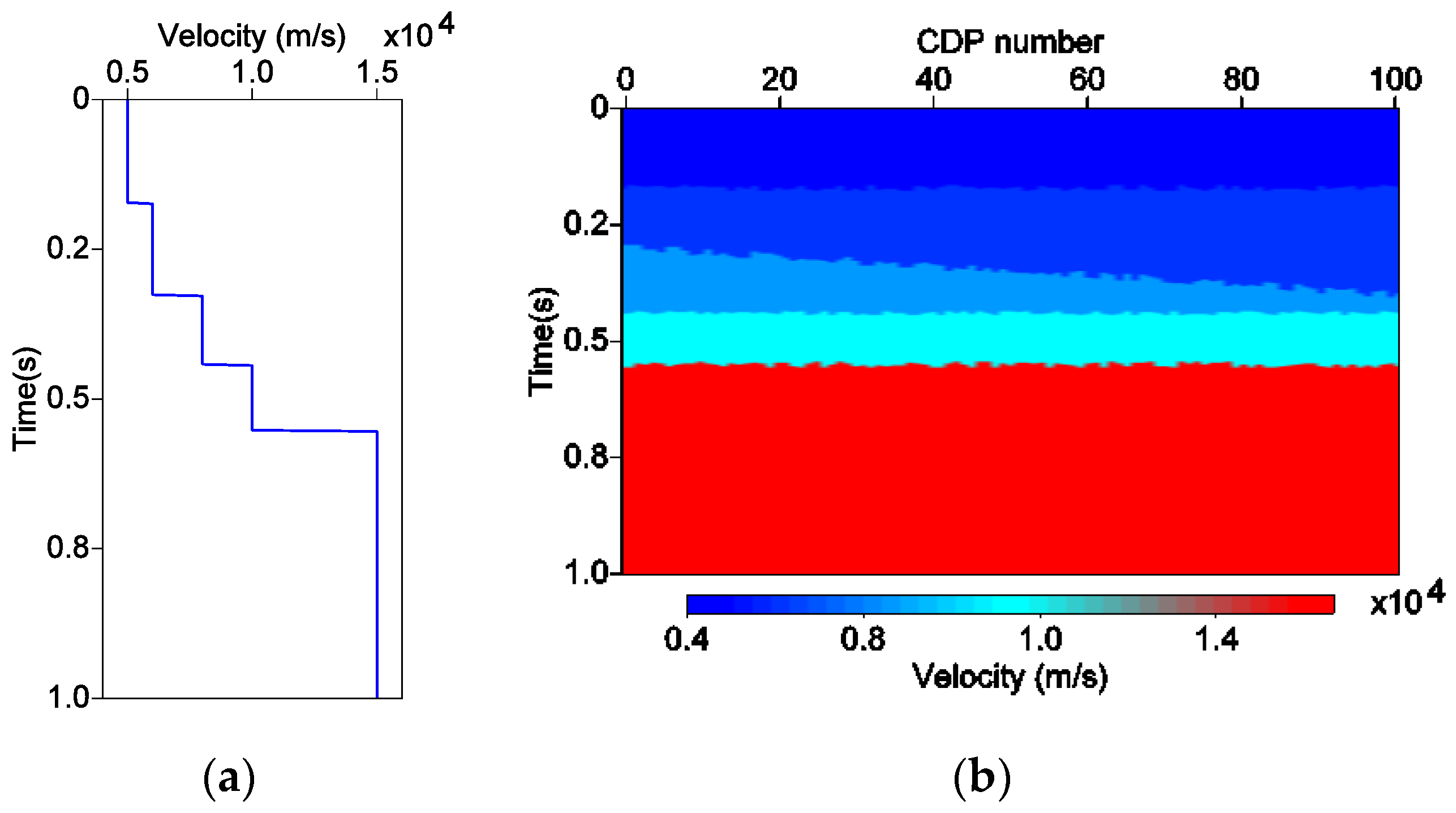
The interval velocity curve is extracted at the theoretical velocity model CDP 30 to simulate the data of a well. The layer velocity curve at CDP 30 is extrapolated under the paths constraint shown in Figure 10 to obtain a interval velocity model, as shown in Figure 11, which is consistent with the theoretical model shown in Figure 4. The vertical difference is because the theoretical velocity model is in depth domain and the extrapolation result is in time domain.
4. Real Data Applications
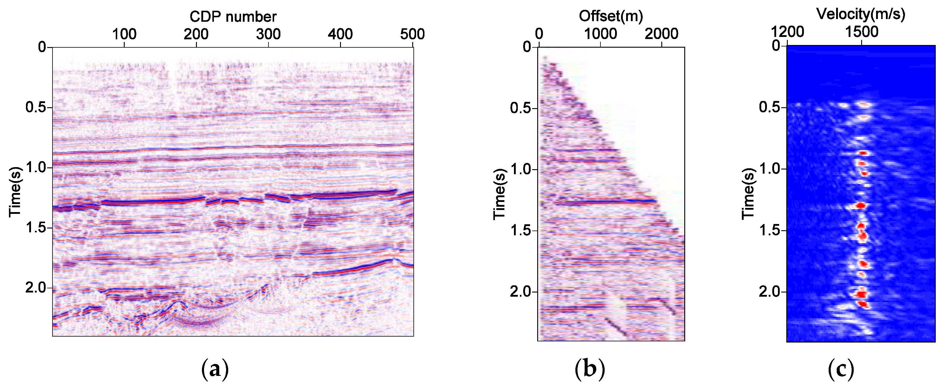
In the real data test, we used the land seismic data from eastern China. The CRP gathers after prestack time migration were used to generate velocity spectra. The number of CRP gathers was 500. The maximum offset was 2200 m. The longitudinal time was 2.5 s. The sampling interval was 2 ms. The stack section is shown in Figure 12a. Figure 12b is the CRP gather at CDP 203, and Figure 12c is the velocity spectrum at CDP 203.
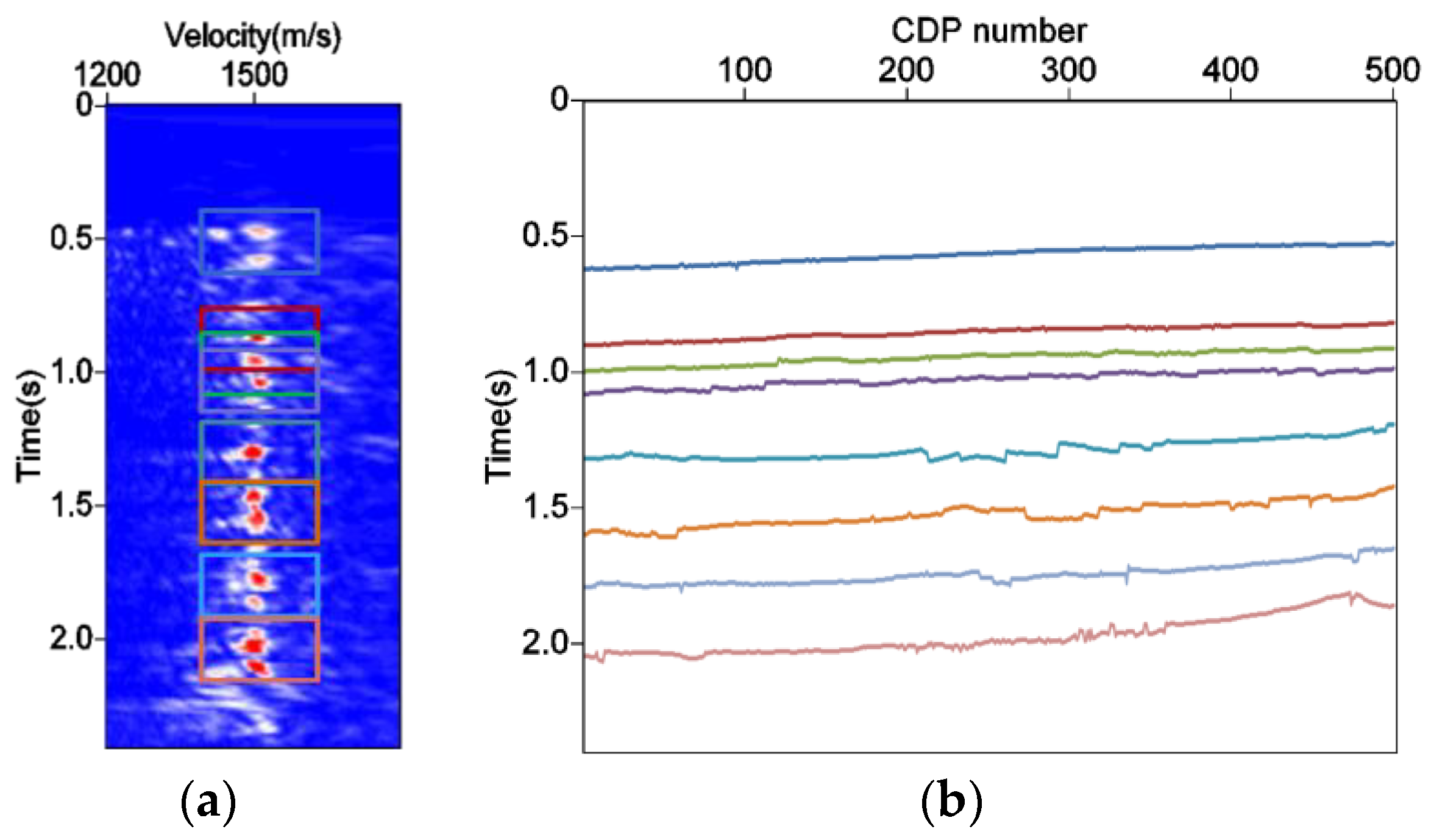
The velocity spectrum at CDP 203 was used as the tracking target of the training data set. Since there was no obvious boundary between the energy clusters in the velocity spectrum in Figure 12, we used the sliding window to realize the target tracking. The time window length is given as 250 ms. The tracking windows are shown in Figure 13a. The real data samples were made in the same way as the theoretical data. The training process had 500 iterations, and the learning rate was set to 0.0001. The position of the window was changed and the same training process repeated until the tracking of the target in the whole time range was completed. The tracking results of all CDP points were connected to form the final tracking paths as shown in Figure 13b. Comparing Figure 13b with Figure 12a, the tracking paths are consistent with the interfaces. The faults between CDP 200–CDP 350 and 1.3–1.8 s can be correctly identified on the tracking results. Along the tracking path, the parameter to be inversed can be extrapolated from the well, and the initial inversion model consistent with the structure can be obtained.
5. Discussions
This method also has some application limitations. Because the characteristics of the energy clusters in the velocity spectrum are closely related to the reflection characteristics of the formation, the method can obtain ideal tracking results when the reflection characteristics from the same formation interface are relatively stable in lateral. In contrast, if the reflection characteristics of the formation change dramatically in lateral, the velocity spectrum tracking will be unstable and the results may be multi-solution. This requires manual intervention or adding constraints to obtain reliable tracking results, such as limiting the trend of the tracking path within a certain range or limit the maximum change of the tracking results of adjacent traces. In addition, if the signal-to-noise ratio of real seismic data is very low, the velocity spectrum features will not be significant, and it will be difficult to extract features and track targets.
In the velocity spectrum tracking of real seismic data, there may be difficulties such as unclear clusters features or background interference. In these cases, the accuracy of target tracking can be improved by changing the window length. The tracking task can be carried out with different window lengths, and the corresponding similarity results will be output for each window length. The results with the highest similarity can be extracted and combined as the final target tracking result.
The extrapolation path of geophysical parameters can be obtained by lateral tracking of velocity spectrum, which can be used as a constraint framework to construct the initial model. The essence of the method is the similarity of the characteristics of velocity spectrum in lateral, that is, the invariable part of the velocity spectrum. In fact, the characteristics of the velocity spectrum have certain changes in lateral, and this change also represents the lateral changes of geophysical parameters to a certain extent. In the absence of gooddata, how to make full use of the characteristics of velocity spectrum to provide more geophysical information will be the next possible research direction.
6. Conclusions
A lateral tracking method of velocity spectrum based on a triple Siamese network structure is proposed in this paper. With this method, the positions of the target image on the velocity spectrum of each CDP can be tracked. The results of the tracking paths can constrain the lateral extrapolation of seismic parameter to establish an initial inversion model, for example, an initial velocity model for prestack depth migration or P-wave, S-wave and density models for elastic parameters inversion. The method does not depend on the interpretation horizons and manual annotation samples. The theoretical and practical results show that the method can efficiently generate the initial model that conforms to the seismic structure and stratigraphic characteristics without the constraint of interpreted horizon data.
Author Contributions
Methodology, L.S.; validation, L.S. and L.D.; writing—original draft preparation, L.S.; writing—review and editing, L.D. and X.W. All authors have read and agreed to the published version of the manuscript.
Funding
This work was supported by the National Natural Science Foundation of China (grantno. 42204128).
Institutional Review Board Statement
Not applicable.
Informed Consent Statement
Not applicable.
Data Availability Statement
The data presented in this study are available on request from the corresponding author.
Conflicts of Interest
The authors declare no conflict of interest.
References
- Mallet, J.L. Geomodeling; Oxford University Press: Oxford, UK, 2002. [Google Scholar]
- Caumon, G.; Collon-Drouaillet, P.; de Veslud, C.L.C.; Viseur, S.; Sausse, J. Surface-based 3D modeling of geological structures. Math. Geosci. 2009, 41, 927–945. [Google Scholar] [CrossRef] [Green Version]
- Hampson, D.; Todorov, T.; Russell, B. Using multi-attribute transforms to predict log properties from seismic data. Explor. Geophys. 2000, 31, 481–487. [Google Scholar] [CrossRef]
- Hansen, T.M.; Mosegaard, K.; Pedersen-Tatalovic, R.; Uldall, A.; Jacobsen, N.L. Attribute-guided well-log interpolation applied to low-frequency impedance estimation. Geophysics 2008, 73, R83–R95. [Google Scholar] [CrossRef] [Green Version]
- Dave, H. Image-guided 3D Interpolation of Borehole Data. In SEG Technical Program Expanded Abstracts 2010; Society of Exploration Geophysicists: Houston, TX, USA, 2010; pp. 1266–1270. [Google Scholar]
- Hale, D.; Wu, X. Horizon volumes with interpreted constraints. Geophysics 2015, 80, IM21–IM33. [Google Scholar]
- Karimi, P.; Fomel, S.; Zhang, R. Creating detailed subsurface models using predictive image-guided well-log interpolation. Interpreatation 2017, 5, T279–T285. [Google Scholar] [CrossRef]
- Hoyes, J.; Cheret, T. A review of “global” interpretation methods for automated 3D horizon picking. Lead. Edge 2011, 30, 38–47. [Google Scholar] [CrossRef]
- Harrigan, E.; Kroh, J.; Sandham, W.; Durrani, T. Seismic Horizon Picking Using an Artificial Neural Network. In Proceedings of the IEEE International Conference on Acoustics, Speech, and Signal Processing, San Francisco, CA, USA, 23–26 March 1992; pp. 105–108. [Google Scholar]
- Leggett, M.; Sandham, W.A.; Durrani, T.S. 3D horizon tracking using artificial neural networks. First Break 1996, 14, 413–418. [Google Scholar] [CrossRef]
- Huang, Y.; Di, H. Dip Interpolation for Improved Multitrace Seismic-Attribute Analysis. In Proceedings of the 2017 SEG International Exposition and Annual Meeting, Houston, TX, USA, 29 September 2017. [Google Scholar]
- Fehmers, G.C.; Höcker, C.F. Fast structural interpretation with structure-oriented filtering. Lead. Edge 2002, 21, 238–243. [Google Scholar] [CrossRef]
- Yu, Y. Automatic Horizon Picking In 3D Seismic Data Using Optical Filters And Minimum Spanning Tree (Patent Pending). In SEG Technical Program Expanded Abstracts 2011; Society of Exploration Geophysicists: Houston, TX, USA, 2011; pp. 965–969. [Google Scholar]
- Wu, H.; Zhang, B.; Lin, T.; Cao, D.; Lou, Y. Semiautomated seismic horizon interpretation using the encoder-decoder convolutional neural network. Geophysics 2019, 84, B403–B417. [Google Scholar] [CrossRef]
- Neidell, N.S.; Taner, M.T. Semblance and Other Coherency Measures for Multichannel Data. Geophysics 1971, 36, 482. [Google Scholar] [CrossRef]
- Krizhevsky, A.; Sutskever, I.; Hinton, G.E. Imagenet classification with deep convolutional neural networks. Adv. Neural Inf. Process. Syst. 2012, 25, 1097–1105. [Google Scholar] [CrossRef] [Green Version]
- He, K.; Gkioxari, G.; Dollár, P.; Girshick, R. Mask r-cnn. In Proceedings of the IEEE International Conference on Computer Vision, Venice, Italy, 22–29 October 2017; pp. 2961–2969. [Google Scholar]
- Li, Y.; Qi, H.; Dai, J.; Ji, X.; Wei, Y. Fully Convolutional Instance-Aware Semantic Segmentation. In Proceedings of the IEEE Conference on Computer Vision and Pattern Recognition, Honolulu, HI, USA, 21–26 July 2017; pp. 2359–2367. [Google Scholar]
- Wang, W.; George, A.M.; Ma, J.; Xie, F. Automatic velocity picking from semblances with a new deep-learning regression strategy: Comparison with a classification approach. Geophysics 2021, 86, 1942–2156. [Google Scholar] [CrossRef]
- Araya-Polo, M.; Dahlke, T.; Frogner, C.; Zhang, C.; Poggio, T.; Hohl, D. Automated fault detection without seismic processing. Lead. Edge 2017, 36, 208–214. [Google Scholar] [CrossRef]
- Bromley, J.; Guyon, I.; LeCun, Y.; Säckinger, E.; Shah, R. Signature verification using a “siamese” time delay neural network. Int. J. Pattern Recognit. Artif. Intell. 1993, 7, 669–688. [Google Scholar] [CrossRef] [Green Version]
- Hadsell, R.; Chopra, S.; LeCun, Y. Dimensionality Reduction by Learning an Invariant Mapping. In Proceedings of the 2006 IEEE Computer Society Conference on Computer Vision and Pattern Recognition (CVPR’06), New York, NY, USA, 17–22 June 2006; pp. 1735–1742. [Google Scholar]
- Vries, D.D.; Berkhout, A.J. Velocity analysis based on minimum entropy. Geophysics 1984, 49, 2132. [Google Scholar] [CrossRef] [Green Version]
- Biondi, B.L.; Kostov, C. High-resolution velocity spectra using eigen structure methods. Geophysics 1989, 54, 832–842. [Google Scholar] [CrossRef] [Green Version]
- Key, S.C.; Smithson, S.B. New approach to seismic-reflection event detection and velocity determination. Geophysics 1990, 55, 1057. [Google Scholar] [CrossRef]
- Fomel, S. Velocity analysis using AB semblance. Geophys. Prospect. 2009, 57, 311–321. [Google Scholar] [CrossRef] [Green Version]
- Luo, S.; Hale, D. Velocity analysis using weighted semblance. Geophys. J. Soc. Explor. Geophys. 2012, 77, U15–U22. [Google Scholar] [CrossRef]
- Ursin, B.; da Silva, M.G.; Porsani, M.J. Generalized Semblance Coefficients Using Singular Value Decomposition. In Proceedings of the 13th International Congress of the Brazilian Geophysical Society & EXPOGEF, Rio de Janeiro, Brazil, 26–29 August 2013; pp. 1544–1549. [Google Scholar]
- Ebrahimi, S.; Kahoo, A.R.; Chen, Y.; Porsani, M. A high-resolution weighted AB semblance for dealing with amplitude-variation-with-offset phenomenon. Geophysics 2017, 82, V85–V93. [Google Scholar] [CrossRef]
- Araya-Polo, M.; Jennings, J.; Adler, A.; Dahlke, T. Deep-learning tomography. Lead. Edge 2018, 37, 58–66. [Google Scholar] [CrossRef]
- Ma, Y.; Ji, X.; Fei, T.W.; Luo, Y. Automatic Velocity Picking with Convolutional Neural Networks. In Proceedings of the 2018 SEG International Exposition and Annual Meeting, Anaheim, CA, USA, 14–19 October 2018. [Google Scholar]
- Zhang, H.; Zhu, P.; Gu, Y.; Li, X. Automatic Velocity Picking Based on Deep Learning. In SEG Technical Program Expanded Abstracts; Society of Exploration Geophysicists: Houston, TX, USA, 2019; pp. 2604–2608. [Google Scholar]
- Schneider, M.; Chang, S.F. A Robust Content Based Digital Signature for Image Authentication. In Proceedings of the International Conference on Image Processing (ICIP), Lausanne, Switzerland, 19 September 1996; pp. 227–230. [Google Scholar]
Figure 1.
Consistency between energy clusters in velocity spectrum and formation interfaces. (a) CDP gather at CDP 30; (b) velocity spectrum generated from the gather shown in (a); (c) stack section.
Figure 1.
Consistency between energy clusters in velocity spectrum and formation interfaces. (a) CDP gather at CDP 30; (b) velocity spectrum generated from the gather shown in (a); (c) stack section.

Figure 2.
Similarity of adjacent velocity spectra. (a) Velocity spectrum of CD P32; (b) velocity spectrum of CDP 34; (c) velocity spectrum of CDP 36.
Figure 2.
Similarity of adjacent velocity spectra. (a) Velocity spectrum of CD P32; (b) velocity spectrum of CDP 34; (c) velocity spectrum of CDP 36.

Figure 3.
Structure of the triple velocity spectrum tracking network.

Figure 4.
Theoretical model of interval velocity.

Figure 5.
CDP gathers at different positions. (a) CDP 30; (b) CDP 50; (c) CDP 70.

Figure 6.
Velocity spectrum. (a) CDP 30; (b) CDP 50; (c) CDP 70.

Figure 7.
Examples of positive sample. (a) Tracking target image; (b) image after 1.5 times stretching; (c) image after 3 times stretching; (d) image after low-pass filtering; (e) image after bandpass filtering; (f) image after high pass filtering.
Figure 7.
Examples of positive sample. (a) Tracking target image; (b) image after 1.5 times stretching; (c) image after 3 times stretching; (d) image after low-pass filtering; (e) image after bandpass filtering; (f) image after high pass filtering.


Figure 8.
Examples of negative sample.

Figure 9.
The tracking results of CDP 50 to CDP 55.

Figure 10.
Result of tracking paths.

Figure 11.
(a) Interval velocity curve at CDP 30; (b) extrapolation velocity result under the paths constraint.
Figure 11.
(a) Interval velocity curve at CDP 30; (b) extrapolation velocity result under the paths constraint.

Figure 12.
(a) Stack section; (b) CRP gather at CDP 203; (c) velocity spectrum at CDP 203.

Figure 13.
(a) Tracking windows; (b) the result of tracking paths.


Table 1.
Network parameters.
| Network Layers | Conv1 | Pool1 | Conv2 | Pool2 | Conv3 | Conv4 | Conv5 |
|---|---|---|---|---|---|---|---|
| Convolution kernel | 11 × 11 | 3 × 3 | 7 × 7 | 3 × 3 | 3 × 3 | 3 × 3 | 3 × 3 |
| Step size | 2 | 2 | 2 | 2 | 1 | 1 | 1 |
Publisher’s Note: MDPI stays neutral with regard to jurisdictional claims in published maps and institutional affiliations. |
© 2022 by the authors. Licensee MDPI, Basel, Switzerland. This article is an open access article distributed under the terms and conditions of the Creative Commons Attribution (CC BY) license (https://creativecommons.org/licenses/by/4.0/).
Share and Cite
MDPI and ACS Style
Sun, L.; Ding, L.; Wang, X. Research on Initial Model Construction of Seismic Inversion Based on Velocity Spectrum and Siamese Network. Appl. Sci. 2022, 12, 10593. https://0-doi-org.brum.beds.ac.uk/10.3390/app122010593
AMA Style
Sun L, Ding L, Wang X. Research on Initial Model Construction of Seismic Inversion Based on Velocity Spectrum and Siamese Network. Applied Sciences. 2022; 12(20):10593. https://0-doi-org.brum.beds.ac.uk/10.3390/app122010593
Chicago/Turabian StyleSun, Luping, Ling Ding, and Xiangchun Wang. 2022. "Research on Initial Model Construction of Seismic Inversion Based on Velocity Spectrum and Siamese Network" Applied Sciences 12, no. 20: 10593. https://0-doi-org.brum.beds.ac.uk/10.3390/app122010593
Note that from the first issue of 2016, this journal uses article numbers instead of page numbers. See further details here.