
A Two-Stage Semi-Supervised High Maneuvering Target Trajectory Data Classification Algorithm

1
Department of Information System Engineering, PLA Strategic Support Force Information Engineering University, Zhengzhou 450001, China
2
China Communications Construction Fourth Engineering Bureau Co., Ltd., Zhengzhou 450001, China
*
Author to whom correspondence should be addressed.
†
The authors contributed equally to this work and co-first authors.
Appl. Sci. 2022, 12(21), 10979; https://0-doi-org.brum.beds.ac.uk/10.3390/app122110979
Submission received: 31 August 2022
/
Revised: 19 October 2022
/
Accepted: 27 October 2022
/
Published: 29 October 2022
(This article belongs to the Special Issue Machine Learning Applications in Transportation Engineering)
Abstract
:Labeled data in insufficient amounts and missing categories are two observable features for high maneuvering target trajectory data. However, the existing research achievements are insufficient for solving these two problems simultaneously during data classification. This study proposed a two-stage semi-supervised trajectory data classification algorithm. By pre-training the autoencoder and combining it with the Siamese network, a two-stage joint training was formed, which enabled the model to deal with missing categories by clustering and maintaining the classification ability under the missing label categories. The experimental simulation results showed that the performance of this algorithm was better than the classical semi-supervised algorithm label propagation and transferred learning when the amount of various labeled data was as low as 1–5. The two-stage training model also had a good effect on the problem of missing categories. When 75% of the types were missing, the purity could still reach 82%, which was about eight percentage points higher than the directly trained network. When two problems appeared simultaneously, compared with the directly trained network, the performance improved by about three percentage points on average, and the purity was consistently higher than the clustering results. In summary, this algorithm was more tolerant of the problems of labeled datasets, so it was more practical.
1. Introduction
Trajectory data records the temporal and spatial changes of moving objects, contains rich temporal and spatial information, and has extremely high analytical value.
The data of high maneuvering target trajectories, such as aircraft and ships performing exploration tasks or search and rescue, compared with conventional trajectories, have two observable features. First, these data are difficult to label and relatively small in scale, so the amount of labeled data is often insufficient. Second, the behavior law of high maneuvering targets rapidly changes in time and space, so the data is quickly updated. However, manual labeling is difficult as a way of updating the labeled dataset in real-time. Therefore, in such trajectory datasets, insufficient quantity and missing categories become too difficult in data processing.
With the development of machine learning and deep learning, the use of neural networks for trajectory classification has gradually become mainstream. For example, both [1,2] used an RNN (recurrent neural network) to extract trajectory features for clustering and classification of trajectories. Both obtained performances superior to traditional classification methods such as decision trees or support vector machines in experiments. In addition, other deep neural networks have also been used for trajectory classification, such as LSTM (long short-term memory) in [3], GRU (gate recurrent unit) in [4], and CNN (convolutional neural networks) in [5,6]. These algorithms have also achieved excellent results in the corresponding trajectory classification applications.
However, training deep network models requires a large amount of high-quality labeled data, which is difficult to directly use in the upper condition [7].
Aiming at the problem of insufficient label data, existing algorithms have abundant research results. For example, Wang et al. [8] addressed this problem using a transfer learning approach, training the model on a dataset similar to the base model. In [9], Yang et al. made full use of unlabeled data to pre-train a feature extraction network and train a classifier on this basis. Ju et al. [10] used data augmentation to solve the problem of too few labels and used GAN (generative adversarial network) to screen out the data with the same distribution as the labeled data and used the five-label data as new training data. The above methods can effectively reduce the impact of insufficient label data.
However, for the problem of missing categories, the processing power of existing algorithms is insufficient. Most of the existing semi-supervised algorithms are finally trained models or classification models, which can only distinguish the labeled and trained categories. For unlabeled categories, the classification performance will drop significantly. Existing algorithms generally distinguish untrained classes through anomaly detection or separate the classification and clustering processes, resulting in poor classification performance.
So, this is a research direction worthy of attention for strengthening the existing semi-supervised classification algorithms in the field of trajectory classification. In particular, the ability to handle the problem of missing categories in labeled datasets needs to be improved. Therefore, this work studied the semi-supervised trajectory classification problem under the conditions of insufficient label data and missing categories and proposed a two-stage semi-supervised high maneuvering target trajectory data classification algorithm. The algorithm designed a network structure combining the Siamese network and autoencoder and accordingly designed a two-stage model training method. The method first used unlabeled data to pre-train the clustering model to ensure the clustering ability of the model for most of the samples in the target domain. Then it used the data in the labeled dataset to fine-tune the model to improve the model’s processing ability for labeled categories. In the experimental part of the study, the simulation experiments under different conditions proved that the model could effectively deal with the problems of an insufficient amount of label data and missing categories. When there was only the problem of an insufficient amount of label data, the algorithm achieved the same performance as existing semi-supervised algorithms. Furthermore, under the condition of missing categories or when there were two problems at the same time, the performance of the algorithm in this study was better.
To sum up, the main purpose and contribution of this study were to address the problem of missing categories and insufficient numbers of track data label datasets under practical application conditions and propose a classification algorithm suitable for this condition, which was more suitable for applications under practical conditions.
2. Problem Analysis
In order to more intuitively observe the impact of the insufficient amount and missing categories problems of the label datasets, we plotted the loss and classification accuracy of a conventional LSTM [11] classification network during training under the corresponding conditions.
In the experiment, there are 12 types of target data. In order to facilitate the training of the model, it is assumed that there were 12 known types of classification targets. In the case of sufficient label data, 50 pieces of training data were taken for each type, and in the case of insufficient label data, 5 pieces of each class were taken as samples. Under the condition of missing categories, two types of label data were deleted.
After one hot encoding of the labels, the calculation of the loss used the Categorical_Crossentropy function. Categorical_Crossentropy generally cooperated with Softmax for single-label classification, which was suitable for the classification of track types. The calculation formula is as follows:
The formula for calculating the accuracy is as follows:
In the formula, represents the number correctly marked and represents the number wrongly marked.
The experimental results are shown in Figure 1.
The two pictures in Figure 1a are the training curves under the insufficient label data amount condition. Due to the insufficient number of training samples, the curve significantly oscillated. The final training set accuracy stabilized at around 0.8, while the test set accuracy was about ten percentage points lower.
The two pictures in Figure 1b are the training curves under that the label data category missing condition. The training set loss function and accuracy could quickly tend to be optimal, and the training set classification accuracy even reached 100%. However, due to the existence of unlabeled categories in the test set, the accuracy of the test set significantly dropped to only about 60%.
Under the condition that the two above problems existed at the same time, not only was the training set’s effect optimal state difficult to achieve, but also the gap between the effect of the test set and training set was more obvious. In addition, the above training curve was obtained by training the model and drawing under the condition that the actual number of categories was known by default. In practical applications, when there were missing categories in the labeled data, the classification model could not distinguish the untrained categories. The negative effects of unknown classes in the target dataset were more severe than in Figure 1.
To sum up, under semi-supervised conditions, the insufficient amount and missing categories problems of label datasets had a serious impact on the training of classification models. This study dealt with the trajectory classification problem with the above problems, so the algorithm required the ability to reduce the scale of the labeled data that the classification model relied on and the ability to deal with missing categories.
First of all, for the problem of insufficient amount of label data, the solution in this study was to introduce a network structure called a Siamese neural network [12] and make full use of unlabeled data to provide auxiliary information in model training.
A Siamese neural network is a network commonly used in metric learning and semi-supervised problems. It was first proposed in the field of signature verification in reference [12]. It is widely used in face verification, text recognition, and other fields [13]. Its basic structure is shown in Figure 2. A pair of samples are input into two neural networks with the same structure and shared weights, and the paired label data are used for training.
The loss function is called the contrastive loss and is calculated as follows [12]:
In the formula, W is the network weight, and Y is the pairwise label. If the pair of samples X1 and X2 belongs to the same class, Y = 0 otherwise Y = 1. DW is the Euclidean distance between X1 and X2 features. When Y = 0, the model minimizes DW. When Y = 1, if DW is greater than m, do not optimize; if DW is less than m, increase the distance between the two to m.
Therefore, in the feature domain, the distance between similar positive sample pairs is narrowed, and the distance between negative sample pairs is widened, which can effectively measure the network of similarity between samples.
Siamese neural networks can effectively utilize labeled data. The input in the Siamese neural network is a pair of samples, so the training samples can be expanded by the combination of samples. Assuming that there are n trajectory samples, sets of training samples can be formed, which greatly increases the number of trainings and uses a small amount of label data to achieve better training results.
The basic Siamese network model can be trained with labeled data but cannot fully utilize the information of a large number of unlabeled samples in the dataset. Therefore, this study referred to the idea of pre-training and model transfer, used unlabeled data to train the commonly used autoencoder clustering model, and combined the model with a Siamese network. This processing could reduce the difficulty of model training and the degree of dependence on labeled data while laying a solid foundation for further processing of missing categories.
For the problem of missing categories, the key was to deal with unlabeled categories, which was essentially a clustering problem. This required the algorithm to have the ability to cluster unlabeled categories while having the ability to classify labeled categories. This was also one of the reasons why this study chose the structure of the Siamese neural network because the Siamese network can not only use the conventional distance calculation and threshold design method for trajectory classification but also can obtain the distance matrix of the samples through the similarity measure for trajectory clustering. Thus, the classification algorithm was transformed into clustering to ensure the basic processing ability of the algorithm for unmarked categories.
This study further combined the Siamese network and the clustering network to design a two-stage model training algorithm to improve the clustering ability of the basic Siamese network model. The first stage trained the commonly used autoencoder clustering model to ensure the model’s processing ability for unlabeled categories. The second stage used the trained clustering model to form a Siamese neural network and used the label data for fine-tuning to further improve the classification performance of the model. However, under the condition of missing categories, relying too much on the guidance of the labeled dataset can lead to overfitting, making the model only able to classify the labeled categories. Therefore, in the second stage, this study used joint training to simultaneously train the supervised and the unsupervised parts of the model. This ensured that the model training process used label data to guide feature extraction without excessive dependence on label data.
Based on the above analysis, this study proposed a two-stage semi-supervised high maneuvering target trajectory data classification algorithm. The algorithm is introduced in detail below.
3. Algorithms
The overall idea of the algorithm is shown in Figure 3.
The training process is divided into two stages.
The first stage trained the autoencoder network in an unsupervised manner as a pre-trained model. Using the autoencoder to extract features suitable for trajectory clustering ensured that the model could extract the general features of most samples in the target domain and had basic clustering capabilities.
In the second stage, the trained clustering models were formed into a Siamese neural network and fine-tuned with labeled data. The supervised and unsupervised parts of the network were simultaneously trained through the design of a hybrid loss function at fine-tuning. While strengthening the classification ability of label categories, we tried to ensure the model’s ability to extract the overall clustering features.
Finally, the similarity matrix of the target dataset was obtained and clustered according to the Siamese network model. The following describes the specific algorithm model in stages.
3.1. Unsupervised Feature Extraction Based on Autoencoder
The purpose of the first stage, the unsupervised learning process, was to fully use unlabeled data to initially train the model. The required trained model could accurately extract general features in unlabeled samples. We ensured the model had basic clustering capabilities for both labeled and unlabeled categories.
In this study, an autoencoder was constructed to perform feature extraction on trajectory data. Autoencoders are commonly used in trajectory clustering and feature extraction [14]. Its structure is shown in Figure 4.
The autoencoder generally consisted of an encoder and a decoder. The purpose of the encoder was to compress the input data into a latent space representation; the decoder aimed to reconstruct the input data represented by this latent space and express the input information as much as possible.
The purpose of the entire network was to make the output and input as close as possible so that the intermediate feature vector could be guaranteed to correspond well to the input data. Therefore, as long as the error between the input and output was small enough, the entire network achieved the purpose of compressing the input space. The most commonly used function was the MSE (mean squared error) loss function, shown in Equation (4).
In the formula, represents the input sample, and represents the restored sample of the output.
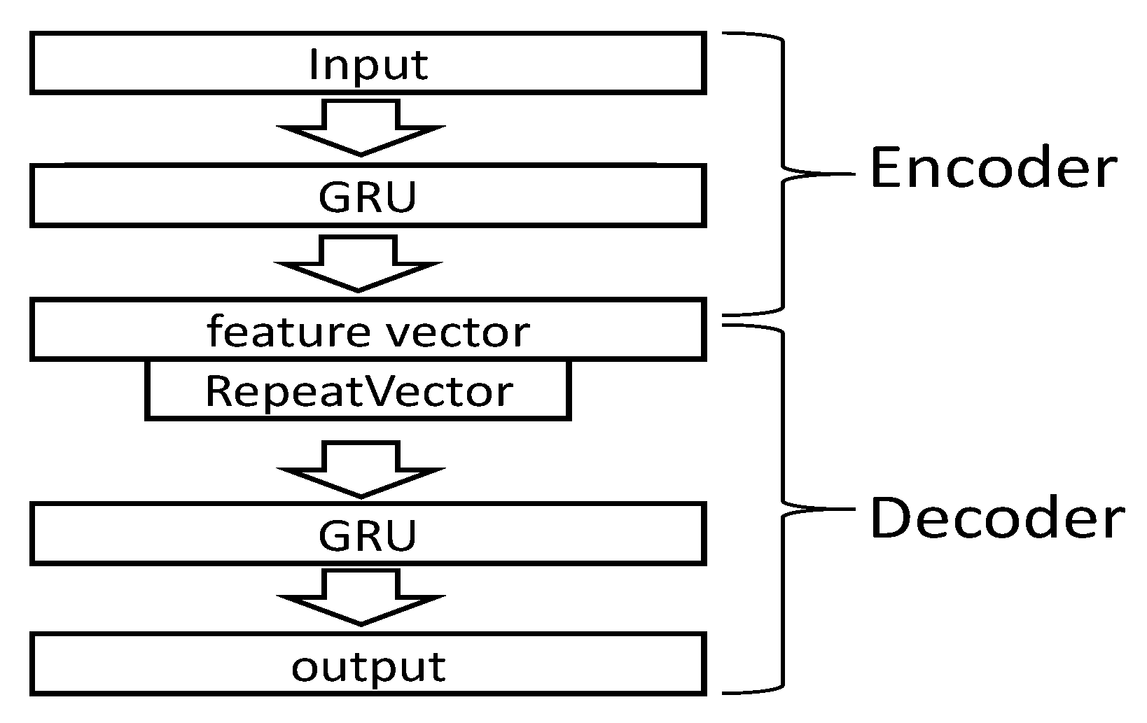
RNN network was the mainstream neural network model for processing time series data. The trajectory sequence was typical time series data [15], and the time series feature was the key piece of information for distinguishing the trajectory type [16]. Therefore, this study used the GRU [17] network structure, a variant of the RNN [18], to build a sequential autoencoder, shown in Figure 5.
In Figure 5, the GRU layer was used to read the timing features of the trajectory. The RepeatVector layer was used to regenerate the time series from the extracted feature vectors and reconstruct the input data using a subsequent symmetric decoder network.
During model training, the input data was normalized. Zero padding was performed to keep the input data length consistent. Taken from the encoder intermediate layer output as the trajectory feature vector. In general clustering algorithms, this feature was used to calculate the similarity for clustering, but because the model lacked guidance, the autoencoder could only blindly extract features during feature extraction. Under the semi-supervised condition of this study, the label data was used to further fine-tune the model in the next stage and improve the model feature extraction effect.
3.2. Classification Feature Enhancement Based on Siamese Network
The second stage was to use the pre-trained autoencoder model to build a Siamese neural network and use the labeled data to train the model’s classification ability for labeled categories. In addition, this fine-tuning could also guide and improve the feature extraction ability of the model.
The model design of the second stage is shown in Figure 6. The main body was the Siamese neural network. The two branches of the Siamese neural network were composed of the encoding network in the pre-trained autoencoder, and the two networks shared weights. The loss in the model consisted of the reconstruction loss of the autoencoder and the output loss of the Siamese network. This was calculated as follows:
Among them, the calculation formula of is shown in Equation (3), and the formulas of Loss1 and Loss2 are shown in Equation (4).
Calculating the two losses at the same time ensured that the network parameters did not have a negative impact on the restoration effect of the autoencoder while using the label data for adjustment, thereby retaining the clustering ability of the first-stage model.
Conventional Siamese neural networks perform classification by calculating similarity and setting thresholds. In this study, the data were processed in a clustering manner, so the Siamese network was used to calculate the similarity of the trajectory data set. Then the similarity matrix was used for clustering. Compared with direct classification, this method better preserved the model’s ability to deal with unlabeled categories.
3.3. Clustering
After the trajectory similarity matrix is extracted according to the method described above, the distance matrix is clustered based on the K-means algorithm. The brief process is shown in Figure 7.
It is worth noting that this paper uses the k-means algorithm under the condition of labels, which can select the initial cluster center in the labeled data to get a better initial center distribution so as to obtain faster clustering speed and better clustering performance.
This paper only uses the basic clustering algorithm to compare the effectiveness of the obtained similarity matrix. In practical applications, the clustering method can be changed according to the application conditions.
4. Experiment and Analysis
In this section, the principle and effect of the algorithm were experimentally verified, mainly to verify the two capabilities of the algorithm: (1) The algorithm’s ability to handle the problem of insufficient label data amount and (2) the algorithm’s ability to deal with the problem of missing label data categories.
4.1. Performance Indicators
Considering that there were some unlabeled categories in the dataset, this study selected clustering metrics to measure the accuracy of the results. The evaluation indicators of clustering selected purity [19] and KL (Kullback-Leible) divergence [20].
Purity is the most intuitive evaluation index to measure the clustering effect simple and transparent. Its calculation formula is similar to the accuracy rate commonly used in classification. First, the correspondence between clusters and classes needed to be assigned. The class with the most samples in the cluster was taken as the representative class of the cluster. This was calculated as follows:
In the formula, N represents the total number of samples; represents the clustered class; represents the correct class; represents all samples in the corresponding cluster after clustering; represents the real samples of this class. The value range of purity is [0,1].
The concept of KL divergence could be used to measure the difference between two distributions. The smaller the difference between the two distributions, the smaller the KL divergence. Its calculation formula is as follows:
In the formula, p and q represent the category distribution of the clustering results and the distribution of actual samples, respectively. The smaller the KL divergence, the more similar the distribution of clustering results was to the actual distribution.
Among them, purity was used to intuitively measure clustering results, and KL divergence was used to observe the overall distribution of results. The combination of the two indicators could make a clearer judgment on the clustering effect.
4.2. Data Sources
The lack of labeled data and missing categories under actual conditions were inconvenient to quantify, so it was difficult to control variables in experiments. Therefore, this study artificially generated corresponding simulation datasets based on actual data to simulate different application conditions.
The original data in the experiment were the civil aviation trajectory data recorded by the ADS-B (Automatic Dependent Surveillance-Broadcast) system [21], which was downloaded from the (https://flightadsb.variflight.com, accessed on 1 March 2021) website, including flight number, time, latitude and longitude, altitude, speed, heading angle, and other information. To reduce the variables in the experiment, this study only retained the two most basic spatiotemporal features of time and location in the data and normalized them. After preprocessing, such as filtering, interpolation, filtering, and smoothing, taking the channel as the category label, the trajectories on the 12 complex routes were taken to create a simulated trajectory dataset. The original trajectory latitude and longitude images are shown in Figure 8a, and the normalized trajectory images are shown in Figure 8b.
Based on the above datasets, different application conditions were simulated by controlling the number of samples and categories of the labeled datasets.
4.3. Model Training Process Validation
One of the problems faced in Siamese network training is the imbalance of training samples. The training samples were composed of pairs of input data, but the number of training samples that were composed of the same pieces was less than that consisting of different types of samples. Unbalanced training data might lead to a decrease in model training performance. Therefore, the training sample pairs composed of the same category were artificially added to ensure the practical effect. We ensured that positive and negative samples had relatively balanced training probabilities. The clustering results of the two methods, comparing taking and not taking treatment measures, are shown in Table 1. It can be seen that this treatment could effectively improve the processing effect of the Siamese network model.
Then, the model training process was tested to prove that the model could normally train and work. The accuracy and loss curves during the two-stage model training process were plotted as shown in Figure 9.
Figure 9a is the variation of the loss with the number of iterations during the training of the first-stage unsupervised autoencoder. It can be seen that as the number of iterations increased, the loss value rapidly dropped and converged, and the final loss value stabilized at a low level. It showed that the model had a good degree of data reduction in the process of encoding and decoding and could effectively extract data features, and the extracted features would not lose too much information.
The change of loss in the second stage of training is shown in Figure 9b. The two curves correspond to the change of loss of the autoencoder and Siamese network parts, respectively. It can be seen that the Siamese network gradually decreased and stabilized with the training loss. The weight parameters of the autoencoder model were migrated, so they were in a low state at the beginning and could remain stable during training.
The similarity matrix obtained by the two models before and after fine-tuning in the second stage was used for dimensionality reduction using the PCA method. Plot PCA plotted to test the effect of the second-stage algorithm. The result is shown in Figure 10:
It can be intuitively seen from Figure 9 that the similarity matrix obtained by the clustering model after the first stage of training could distinguish samples of different categories. However, after the second stage of fine-tuning, the distance distribution between various samples was more reasonable, and the distinction between samples was more effective.
The above chart results show that the two-stage training algorithm designed in this paper can be trained normally and achieve the expected effect at each stage.
4.4. Label Data Amount Insufficient Problem
This section verifies the ability of the algorithm to deal with the problem of insufficient labels and does not consider the problem of unlabeled categories. The label data set used was consistent with the target data set trajectory category.
It was generally considered that less than 10 labels for each category were the condition of few labels. Firstly, the influence of different amounts of labeled data on the algorithm of this study was studied, and the robustness of the algorithm to the problem of few labels was tested. The statistical results are shown in Table 2.
As can be seen from the table, with the reduction of various label data, the overall clustering purity slowly decreased, and the KL divergence kept fluctuating at a low level, indicating that the overall effect of clustering was maintained at a high level. Even under the extreme condition that the number of labels for each type of data was 1, the performance could be significantly improved compared with the last unlabeled clustering model. It showed that the algorithm in this study could effectively utilize the label data and was robust in the reduction of label data.
First, we observed the model loss curve in the algorithm training process, compared it with the general classification model training curve, and conducted experiments with five label data for each category. The results are shown in Figure 11.
Figure 11 show the change of the loss curve during the training of the two algorithms on the same few-label dataset. Although it cannot be numerically compared due to the different models and loss functions, it can be clearly seen that during the training process of the model in this paper, the training set and test set losses were closer. It shows that the model in this paper uses the label data more reasonably, and the possibility of overfitting is lower.
Then, the algorithm in this study was compared with other classic semi-supervised algorithms to test the ability of the algorithm to utilize label data. The comparison algorithm selected the label propagation algorithm [22] and the GRU migration model algorithm.
The label propagation algorithm is a popular semi-supervised clustering method. The principle is to use the labeled data as the starting point, calculate the distance between samples, and judge the samples with closer distances as the corresponding category. In this paper, DTW [23] distance is used for label propagation. Compared with unsupervised clustering methods, label propagation algorithms can make better use of labeled data and significantly improve clustering accuracy.
Another comparison algorithm referred to the algorithm principle in [9], which used unlabeled data to train a clustering model to provide auxiliary information and then transferred the model to a classification network for fine-tuning. Hereafter, this paper calls it the GRU migration model. The general idea of this model is similar to this study; the main difference lies in the Siamese neural network and the handling of the missing category problem. Comparing our algorithm with this algorithm, we could test the working effect of the Siamese neural network and the ability of the algorithm to utilize data information.
In addition, the unsupervised clustering and the GRU classification model obtained by direct training were used as comparison algorithms. The statistical clustering effects of the above algorithms are shown in Table 3.
The model for direct clustering and the classification model trained with a small number of labels performed the worst. The reason is that both algorithms do not make full use of known information and only use unlabeled data or labeled data, respectively. The effect of the classification model trained under the condition of few labels was even worse than the clustering model, indicating that the amount of label data under this experimental condition was too small to reflect the characteristics of the dataset, and the classification model could not be effectively trained.
The performance of the two semi-supervised classification algorithms was significantly improved. The GRU migration model algorithm made full use of the pre-training information provided by unlabeled data, which effectively reduced the difficulty of training the classification model and alleviated the problems caused by insufficient labeled data, but this method had limitations. As shown in Table 3, under the extreme condition that the amount of all kinds of label data was 1, too little label data brought negative effects to the original clustering model, which reduced the performance compared with the clustering algorithm. The label propagation algorithm also required the number of labels. Under the condition that the amount of label data was 1, this method was essentially equivalent to the k-means algorithm for determining the initial cluster center. The effect of two semi-supervised classification algorithms, label propagation and transfer training, was significantly improved. These two semi-supervised algorithms were regarded as enhancements to the clustering and directly trained classification models, which better synthesized the label dataset and target data to improve classification performance.
However, the algorithm designed in this study achieved comparable or even better results than the two classical semi-supervised algorithms under the general low-label situation with five labeled data. The advantage was more obvious under the condition of extremely few labels. Therefore, based on the above analysis, it was proven that methods such as twinning network clustering and two-stage training designed in this study effectively utilized label data and were excellent semi-supervised classification algorithms. It was an excellent semi-supervised classification algorithm.
4.5. Label Data Category Missing Problem
The processing capability for labeled categories has been verified in the previous section. This section further examines the clustering ability of the algorithm for unlabeled categories in the target dataset.
For categories with missing labels, the classification model could effectively classify, and the classification accuracy was greatly reduced, so this section will no longer use the label propagation and GRU classification model as the comparison algorithm. In our algorithm, the processing ability of unlabeled categories in the dataset mainly came from the designed two-stage training method. Therefore, the conventional Siamese neural network training method that does not perform clustering pre-training and directly uses label data to train was selected as a comparison.
We created simulation datasets for the experiments. The condition of missing categories in the labeled dataset was simulated by removing the entire class of data in the labeled dataset.
First, under the conditions of the same learning rate and the number of iterations, we compared the training processes of the two methods in the categories of complete label and missing label datasets, as shown in Figure 12.
From the loss curve plotted in Figure 12, it can be seen that in the labeled dataset with complete categories, both algorithms could obtain lower losses through training. However, the training process of the model directly trained was unstable, and the loss of final convergence was larger. The gap between the test set and training set results was larger, indicating that it was more prone to overfitting. In contrast, the initial loss in the training process of the two-stage model designed in this study was smaller, so the training convergence was faster. This advantage was even more pronounced on incomplete labeled datasets. The above results showed that the two-stage fine-tuning method designed in this paper was beneficial to the training of the model and was more robust in the problem of missing categories.
After that, datasets with different proportions of missing labels were made, the missing categories were selected by cross-validation, and the average value was obtained after multiple experiments. Table 4 shows the clustering results of the above two algorithms under different missing ratios in the statistical label dataset.
As can be seen from Table 4, as the number of missing categories in label data increased, the performance of the models trained by the two training methods continuously decreased. However, the two-stage fine-tuning model designed in this study eventually converged in the performance of the general clustering model, while the directly trained model fell all the way and lost the ability to classify normally. This result proved that the algorithm in this study successfully combined the clustering and classification models, which ensured that the label data was used to improve the classification effect of the model without losing the previous clustering performance of the model.
In addition, from the results of 100% category completeness in Table 4, it can be seen that the network trained in two stages still has a better classification effect in the absence of the missing category problem. This was because the training method based on the clustering model had better initial weights and could find the optimal solution during training more quickly and accurately, while the direct training method initially required more weight adjustment, and the training was more difficult.
In order to compare the classification effect of the algorithm on the unlabeled categories in the dataset more intuitively, the clustering purity of the two classification algorithms for each category of trajectories was plotted, as shown in Figure 13. There were two classes of labels missing from the label dataset, where class 11 and class 12 corresponded to the classes for which labels were removed.
It can be seen that the directly trained model had a rapid decline in classification performance for the two types of unlabeled data, resulting in a serious decline in overall performance. It can be speculated that the reason was the lack of basic weights of the clustering model, which led to the trained Siamese network only having the ability to process the known categories of the label data, resulting in a phenomenon similar to overfitting. It was even possible to classify a category with missing labels and other categories of data as 1, resulting in a decrease in overall performance. Combined with the indicator of purity in Table 4, it was shown that the distribution of the results obtained by the model designed in this study was more reasonable, and the overall processing capability for each category was stronger.
The above experiments prove that the two-stage Siamese neural network classification algorithm designed in this paper can effectively deal with the problem of missing label data categories.
4.6. Comprehensive Performance Analysis
From the results and analysis of Table 3 and Table 4 in the previous two sections, the algorithm’s ability to deal with the problem of insufficient data and missing categories could be generally judged. In order to more intuitively observe the working performance of the algorithm under the condition that there were two kinds of problems at the same time, we used the amount of label data and the completeness rate of label category as the x- and y-coordinates and the purity as the z-axis, and drew a 3-dimensional surface graph, as shown in Figure 14.
Among them, the specific values of the purity results of the two algorithms are shown in Table 5.
The specific result data under the condition that the amount of each label data was 5 and 25% of label categories were missing are shown in Table 6. In addition, the directly trained Siamese neural network and the method of combining the GRU network classification model and autoencoder clustering were used. That is, we first classified the untrained categories as abnormal categories and then used the autoencoder to cluster the abnormal categories as a comparison algorithm.
It can be seen from the data in Table 6 that compared with other semi-supervised algorithms, the model based on the Siamese neural network had obvious advantages. Combining the conclusions of the previous two sections, it was judged that this advantage was mainly reflected in the ability to deal with the problem of missing categories.
Figure 14 shows the comparison of the two methods based on a Siamese neural network. The ordinate in Figure 14 is the clustering purity; the red surface corresponds to the purity change of the algorithm in this study; the blue surface corresponds to the directly trained Siamese neural network; the gray plane represents the unlabeled clustering purity, which is stable at around 0.8. It can be seen from the figure that the two surfaces have no obvious change in the coordinate axis of the data amount, indicating that the two methods both have high robustness in this problem, which was due to the Siamese network effectively dealing with the problem of few labels. However, for the problem of missing categories, the processing capabilities of the two algorithms were significantly different. In the figure, the purity surface of the algorithm in this study always remained above the direct clustering effect, and the classification accuracy of the directly trained Siamese network model was even lower than that of the direct clustering when the missing class rate was high. It showed that the two-stage training method designed in this study could better maintain the clustering effect of the model. It was more robust in the missing class problem.
Compared with the directly trained Siamese network, the two-stage training method designed in this study was more effective, especially in the KL divergence that reflected the overall distribution of the overall clustering results. This was because the method retained the clustering performance obtained by training with a large amount of unlabeled data, so the overall distribution of the obtained results was more reasonable. In summary, the algorithm in this study effectively dealt with the two problems of insufficient numbers and missing categories of labels. Under the corresponding conditions, the clustering purity was higher.
5. Conclusions
Aiming at the problem of insufficient numbers and missing categories of trajectory label datasets, a two-stage semi-supervised high maneuvering target trajectory data classification algorithm was proposed. The algorithm referred to the principles of pre-training models and metric learning methods in the semi-supervised field, combined the autoencoder with the Siamese neural network to design a classification model, and designed a corresponding two-stage model training method.
Experiments showed that the algorithm improved the classification ability by using labeled data and had the ability to cluster unlabeled categories at the same time. It effectively dealt with the special cases of insufficient label data and missing categories. For the problem of missing categories, when only 25% types were labeled, the purity still reached 82%, which is about eight percentage points higher than the directly training the network; when there were two problems at the same time, the purity was maintained at the average above the clustering results. Compared with the directly trained network, the performance improved by about three percentage points on average.
5.1. Practical Application
In this study, a semi-supervised classification algorithm was proposed by fully considering the practical problems of insufficient label data amount and missing categories. We reduced the algorithm’s dependence on labeled data and increased the processing capacity of abnormal track labeled datasets. The algorithm has backward compatibility. When the amount of data marking was sufficient, and the data type marking was not missing, it still achieved a considerable performance index, which could be used for data processing under normal circumstances.
So, this algorithm could be used as a beneficial supplement to the current track data processing system, to enhance the applicability of the system, and to lay the foundation for subsequent applications, such as target identity attribute recognition and behavior monitoring.
5.2. Limitations and Future Developments
The algorithm still has some limitations, which will serve as an improvement direction for future research. For example, the above experiments were conducted under the condition that various types of data were relatively balanced. When the number of various types of samples, especially unlabeled categories, was small, the method was difficult to achieve the recognition effect. At the same time, the two-stage training of the algorithm inevitably brought a larger amount of computation. In addition, further optimization of the network structure of the model and experiments on more datasets deserves further research. The above shortcomings will affect the practical application of the algorithm. Therefore, future research will take these as the direction for improvement.
Author Contributions
Formal analysis, Q.L.; project administration, Q.L.; conceptualization, X.H.; formal analysis, X.H.; writing, X.H.; data curation, K.C. and Q.O.; validation, K.C. and Q.O. All authors have read and agreed to the published version of the manuscript.
Funding
This research received no external funding.
Institutional Review Board Statement
Not applicable.
Informed Consent Statement
Not applicable.
Data Availability Statement
The data used in this paper can be downloaded from https://flightadsb.variflight.com (the data used in this article was downloaded from March to June 2021) or can be obtained by contacting the corresponding author.
Conflicts of Interest
The authors declare no conflict of interest.
References
- Wang, T.; Ye, C.; Zhou, H.; Ou, M.; Cheng, B. AIS Ship Trajectory Clustering Based on Convolutional Auto-encoder. In Intelligent Systems and Applications, Proceedings of the SAI Intelligent Systems Conference, London, UK, 3–4 September 2020; Springer International Publishing: Cham, Switzerland, 2020. [Google Scholar]
- Jiang, X.; de Souza, E.N.; Pesaranghader, A.; Hu, B.; Silver, D.L.; Matwin, S. Trajectoryne: An embedded gps trajectory representation for point-based classifification using recurrent neural networks. In Proceedings of the 27th Annual International Conference on Computer Science and Software Engineering, Markham, ON, Canada, 6–8 November 2017. [Google Scholar]
- Sun, Y. Target recognition of aircraft flight trajectory based on deep learning. In Proceedings of the 1st Annual Conference on Air Traffic Management System Technology, Nanjing, China, 29 November 2018. [Google Scholar]
- Jiang, X.; Liu, X.; de Souza, E.N.; Hu, B.; Silver, D.L.; Matwin, S. Improving point-based AIS trajectory classifification with partition-wise gated recurrent units. In Proceedings of the 2017 International Joint Conference on Neural Networks (IJCNN), Anchorage, AK, USA, 14–19 May 2017. [Google Scholar]
- Yifan, Z.; An, L.; Guanfeng, L.; Zhixu, L.; Qing, L. Deep representation learning of activity trajectory similarity computation. In Proceedings of the 2019 IEEE International Conference on Web Services. (ICWS), Milan, Italy, 8–13 July 2019. [Google Scholar]
- Zhang, R.; Xie, P.; Wang, C.; Liu, G.; Wan, S. Classifying transportation mode and speed from trajectory data via deep multi-scale learning. Comput. Networks 2019, 162, 106861. [Google Scholar] [CrossRef]
- Yu, Y. A Study on Some Problem of Semi-Supervised Learning. Master’s Thesis, Fujian University, Fujian, China, 2010. [Google Scholar]
- Wang, C.; Zhao, J.; Yang, P.; Li, S. Small-Sample SAR Vessel Target Recognition Based on Transfer Learning. Mob. Commun. 2022, 46, 22–27. [Google Scholar]
- Yang, X.; Ding, F.; Zhang, D.; Zhang, M. Vehicular Trajectory Big Data: Driving Behavior Recognition Algorithm Based on Deep Learning. In Artificial Intelligence and Security, Proceedings of the International Conference on Artificial Intelligence and Security, Hohhot, China, 17–20 July 2020; Springer: Singapore, 2020. [Google Scholar]
- Ju, Y.; Li, Q.; Zhao, C.A. Semi-supervised Classification Algorithm for Encrypted Discrete Sequential Protocol Data Based on GAN. In Proceedings of the 2020 IEEE 20th International Conference on Communication Technology, Nanning, China, 28–31 October 2020. [Google Scholar]
- Hochreiter, S.; Schmidhuber, J. Long Short-Term Memory. Neural Comput. 1997, 9, 1735–1780. [Google Scholar] [CrossRef] [PubMed]
- Bromley, J.; Guyon, I.; LeCun, Y.; Säckinger, E.; Shah, R. Signature verification using a “siamese” time delay neural network. Adv. Neural Inf. Process. Syst. 1993, 7, 669–688. [Google Scholar] [CrossRef] [Green Version]
- Bajić, F.; Job, J. Chart classification using siamese CNN. J. Imaging 2021, 7, 220–238. [Google Scholar] [CrossRef] [Green Version]
- Zeng, W.; Xu, Z.; Cai, Z.; Chu, X.; Lu, X. Aircraft Trajectory Clustering in Terminal Airspace Based on Deep Autoencoder and Gaussian Mixture Model. Aerospace 2021, 8, 266. [Google Scholar] [CrossRef]
- Kapadais, K.; Varlamis, I.; Sardianos, C.; Tserpes, K. A Framework for the Detection of Search and Rescue Patterns Using Shapelet Classification. Future Internet 2019, 11, 192. [Google Scholar] [CrossRef] [Green Version]
- Cui, T.; Wang, G.; Gao, J. Ship trajectory classification method based on 1DCNN-LSTM. Comput. Sci. 2020, 47, 176–184. [Google Scholar]
- Cho, K.; Van Merriënboer, B.; Gulcehre, C.; Bahdanau, D.; Bougares, F.; Schwenk, H.; Bengio, Y. Learning phrase representations using RNN encoder-decoder for statistical machine translation. arXiv 2014, arXiv:1406.1078. [Google Scholar]
- Elman, J.L. Finding structure in time. Cogn. Sci. 1990, 14, 179–211. [Google Scholar] [CrossRef]
- Kullback-Leibler Divergence Explained. Available online: https://www.countbayesie.com/blog/2017/5/9/kullback-leibler-divergence-explained (accessed on 10 May 2017).
- Manning, C.D.; Raghavan, P.; Schütze, H. Introduction to Information Retrieval; Cambridge University Press: Cambridgeshire, UK, 2008; pp. 356–360. [Google Scholar]
- Zhang, J.; Liu, W.; Zhu, Y. Study of ADS-B data evaluation. Chin. J. Aeronaut. 2011, 24, 461–466. [Google Scholar] [CrossRef]
- Zhu, X.; Ghahramani, Z.; Lafferty, J. Semi-supervised learning using Gaussian fields and harmonic functions. In Proceedings of the 20th International Conference on Machine Learning, Washington, DC, USA, 21–24 August 2003; pp. 912–919. [Google Scholar]
- Berndt, D.J.; Clifford, J. Using dynamic time warping to find patterns in time-series. In Proceedings of the 3rd International Conference on Knowledge Discovery and Data Mining, Seattle, WA, USA, 31 July 1994–1 August 1994. [Google Scholar]
Figure 1.
Accuracy and loss curves in classification network training. (a1) Accuracy curve under the insufficient amount condition; (a2) loss curves under the insufficient amount condition; (b1) accuracy curve under the categories missing condition; (b2) loss curve under the categories missing condition; (c1) accuracy curve under the insufficient amount and categories missing condition; (c2) loss curve under the insufficient amount and categories missing condition.

Figure 2.
Siamese network structure.

Figure 3.
The overall flow of the algorithm.

Figure 4.
Autoencoder structure.

Figure 5.
Sequence autoencoder network structure.

Figure 6.
The model of stage two.

Figure 7.
k-means clustering process.

Figure 8.
Simulation trajectory dataset. (a) Original trajectory image and (b) normalized trajectory image.
Figure 8.
Simulation trajectory dataset. (a) Original trajectory image and (b) normalized trajectory image.

Figure 9.
Model training process. (a) Stage 1 training loss curve and (b) Stage 2 training loss curve.
Figure 9.
Model training process. (a) Stage 1 training loss curve and (b) Stage 2 training loss curve.

Figure 10.
PCA diagram. (a) PCA diagram before fine-tuning and (b) PCA diagram after fine-tuning.

Figure 11.
Comparison of training loss curves. (a) LSTM classification model training and (b) our algorithm training.
Figure 11.
Comparison of training loss curves. (a) LSTM classification model training and (b) our algorithm training.

Figure 12.
Loss curve during training. (a1) Direct training on the full-label dataset; (a2) direct training on incomplete labeled datasets; (b1) fine-tuning on the full-label dataset; (b2) fine-tuning on the incomplete label dataset.
Figure 12.
Loss curve during training. (a1) Direct training on the full-label dataset; (a2) direct training on incomplete labeled datasets; (b1) fine-tuning on the full-label dataset; (b2) fine-tuning on the incomplete label dataset.

Figure 13.
Classification accuracy of various types of data. (a) Directly Trained model; (b) two-stage trained model.
Figure 13.
Classification accuracy of various types of data. (a) Directly Trained model; (b) two-stage trained model.

Figure 14.
Purity surface plot.


Table 1.
Experimental results of sample balance processing.
| Clustering Algorithm | Purity | KL Divergence |
|---|---|---|
| Siamese network | 0.89 | 0.068 |
| Siamese network (balance adjustment) | 0.937 | 0.046 |
Table 2.
Experimental results of different training samples.
| The Amount of Various Labels | 20 | 10 | 5 | 1 | 0 (Clustering) |
|---|---|---|---|---|---|
| Purity | 0.943 | 0.945 | 0.921 | 0.898 | 0.794 |
| KL divergence | 0.016 | 0.047 | 0.034 | 0.037 | 0.142 |
Table 3.
Experimental results of different algorithms under the condition of few labels.
| Clustering Algorithm | The Labels’ Number Is 5 | The Labels’ Number Is 1 | ||
|---|---|---|---|---|
| Purity | KL Divergence | Purity | KL Divergence | |
| Unsupervised clustering | 0.794 | 0.142 | 0.794 | 0.142 |
| GRU network | 0.780 | 0.133 | 0.650 | 0.304 |
| GRU migration model | 0.916 | 0.042 | 0.785 | 0.067 |
| Label propagation algorithm | 0.909 | 0.022 | 0.821 | 0.077 |
| Our algorithm | 0.921 | 0.034 | 0.883 | 0.037 |
Table 4.
Experimental results under different label category completeness.
| Label Category Completeness | 100% | 75% | 50% | 25% | 0% (Clustering) |
|---|---|---|---|---|---|
| Two-Stage Trained Model | |||||
| Purity | 0.941 | 0.898 | 0.862 | 0.82 | 0.794 |
| KL divergence | 0.012 | 0.021 | 0.049 | 0.115 | 0.142 |
| Directly Trained Model | |||||
| Purity | 0.933 | 0.890 | 0.80 | 0.75 | —— |
| KL divergence | 0.037 | 0.114 | 0.27 | 0.323 | —— |
Table 5.
Purity results.
| Two-Stage Trained Model | ||||
| Label Category Completeness | 1-Label | 5-Label | 10-Label | 20-Label |
| 25% | 0.804 | 0.808 | 0.816 | 0.822 |
| 50% | 0.826 | 0.852 | 0.861 | 0.86 |
| 75% | 0.873 | 0.898 | 0.902 | 0.905 |
| 100% | 0.9 | 0.915 | 0.945 | 0.942 |
| Directly Trained Model | ||||
| Label Category Completeness | 1-Label | 5-Label | 10-Label | 20-Label |
| 25% | 0.744 | 0.759 | 0.773 | 0.77 |
| 50% | 0.763 | 0.819 | 0.836 | 0.84 |
| 75% | 0.869 | 0.884 | 0.885 | 0.9 |
| 100% | 0.9 | 0.903 | 0.905 | 0.933 |
Table 6.
Clustering results.
| Clustering Algorithm | Purity | KL Divergence |
|---|---|---|
| GRU migration model + autoencoder clustering | 0.821 | 0.104 |
| Label propagation algorithm | 0.735 | 0.158 |
| Direct training (Siamese network) | 0.832 | 0.115 |
| Algorithm in this study | 0.885 | 0.077 |
Publisher’s Note: MDPI stays neutral with regard to jurisdictional claims in published maps and institutional affiliations. |
© 2022 by the authors. Licensee MDPI, Basel, Switzerland. This article is an open access article distributed under the terms and conditions of the Creative Commons Attribution (CC BY) license (https://creativecommons.org/licenses/by/4.0/).
Share and Cite
MDPI and ACS Style
Li, Q.; He, X.; Chen, K.; Ouyang, Q. A Two-Stage Semi-Supervised High Maneuvering Target Trajectory Data Classification Algorithm. Appl. Sci. 2022, 12, 10979. https://0-doi-org.brum.beds.ac.uk/10.3390/app122110979
AMA Style
Li Q, He X, Chen K, Ouyang Q. A Two-Stage Semi-Supervised High Maneuvering Target Trajectory Data Classification Algorithm. Applied Sciences. 2022; 12(21):10979. https://0-doi-org.brum.beds.ac.uk/10.3390/app122110979
Chicago/Turabian StyleLi, Qing, Xintai He, Kun Chen, and Qicheng Ouyang. 2022. "A Two-Stage Semi-Supervised High Maneuvering Target Trajectory Data Classification Algorithm" Applied Sciences 12, no. 21: 10979. https://0-doi-org.brum.beds.ac.uk/10.3390/app122110979
Note that from the first issue of 2016, this journal uses article numbers instead of page numbers. See further details here.