Uncertainty-Controlled Remaining Useful Life Prediction of Bearings with a New Data-Augmentation Strategy

Abstract

The remaining useful life (RUL) of bearings based on deep learning methods has been increasingly used. However, there are still two obstacles in deep learning RUL prediction: (1) the training process of the deep learning model requires enough data, but run-to-failure data are limited in the actual industry; (2) the mutual dependence between RUL predictions at different time instants are commonly ignored in existing RUL prediction methods. To overcome these problems, a RUL prediction method combining the data augmentation strategy and Wiener–LSTM network is proposed. First, the Sobol sampling strategy is implemented to augment run-to-failure data based on the degradation model. Then, the Wiener–LSTM model is developed for the RUL prediction of bearings. Different from the existing LSTM-based bearing RUL methods, the Wiener–LSTM model utilizes the Wiener process to represent the mutual dependence between the predicted RUL results at different time instants and embeds the Wiener process into the LSTM to control the uncertainty of the result. A joint optimization strategy is applied in the construction of the loss function. The efficacy and superiority of the proposed method are verified on a rolling bearing dataset obtained from the PRONOSTIA platform. Compared with the conventional bearing RUL prediction methods, the proposed method can effectively augment the bearing run-to-failure data and, thus, improve the prediction results. Meanwhile, fluctuations of the bearing RUL prediction result are significantly suppressed by the proposed method, and the prediction errors of the proposed method are much lower than other comparative methods.

1. Introduction

Rolling bearings as key components are widely used in various machines, such as gearboxes, wind turbines, and so on. The micropitting [1], internal clearance [2], and lubricant contamination [3] are factors that affect the healthy operation of rolling bearings. These factors affect the bearing life through load distribution, frictional torque, generated vibration, and heat. Predicting the remaining useful life (RUL) of bearings is critical to keeping a machine in healthy working order [4]. Current methods for RUL prediction can be divided into several major categories: physics model-based methods, statistical model-based methods, and artificial intelligence (AI)-based methods [5,6]. Among these methods, statistical model-based methods and AI-based methods are widely used in bearing RUL prediction.

The goal of statistical model-based methods is to accurately explain the machine’s degrading process using a statistical model [7]. There are some commonly used statistical models, such as Wiener processes [8], Gamma processes [9,10], and so on. Then, the parameters in the statistical model are estimated by particle filtering [11], expectation maximization algorithm [12], recursive filtering algorithm [13], and so on. The Gamma process and the Inverse Gaussian process, however, are only appropriate for describing monotonous degradation processes. Because of self-healing and small machine repairs, non-monotonous processes are more common in actual industrial settings. The Wiener process is more popular because it can be used both in the monotonous and non-monotonous degradation process. Although statistical model-based methods have implemented several well-established studies in RUL prediction, statistical model-based methods are often developed on a case-specific basis, with the limitation of requiring explicit prior knowledge [14,15].

The AI-based methods can deal with a large amount of monitoring data by machine learning (ML) techniques without much prior knowledge. Traditional machine learning techniques, such as Support Vector Machine (SVM) [16,17] and Relevance Vector Machine (RVM) [18], have been widely used in RUL prediction. Compared with the traditional machine learning techniques, deep learning methods show greater potential in dealing with high non-linearity and data complexity. There are some commonly used deep learning (DL) models, such as Auto-Encoder (AE) [19], Convolutional Neural Network (CNN) [20,21,22,23,24], Recurrent Neural Network (RNN) [25], and so on. Zhao et al. [26] used CNN in bearing RUL prediction. Raw signals are transformed into the time-frequency domain features and then mapped with the RUL by the 2D-CNN model. The Long Short-Term Memory Neural Network (LSTM) network is one of the RNN variations that can address the issue of gradient disappearance and gradient explosion. Xiang et al. [27] proposed an LSTM with attention mechanism for gear RUL prediction, calculating the contribution of the input during the RUL prediction by using the attention mechanism to improve the performance of the network. However, the AI-based methods still have two limitations: (1) the training process of AI-based methods requires enough data; Thus, lacking run-to-failure data limits the training process. (2) The RUL prediction by the existing deep learning model at different times is mutually independent. The RUL prediction sequence is always ignored in this way.

In order to get the sufficient data for deep learning model, several data augmentation techniques have been applied in fault diagnosis [28] and RUL prediction [29]. Generative Adversarial Networks (GANs) have been widely used to solve the problem of data imbalance in fault diagnosis [30,31]. Behera et al. [32] proposed a RUL prediction method based on conditional generative adversarial network (CGAN) and deep gated recurrent unit (DGRU) network. Hundreds of run-to-failure data were used to train the CGAN to generate more data. Then, the DGRU was applied to predict the RUL. However, GAN models still require enough data to train, which is not suitable when only several run-to-failure samples are offered.

The RUL prediction sequence is rarely considered in the existing DL-based models. Thus, the uncertainty between the predicted result at different times is always ignored [33]. The accuracy of the predicted result is the only object in the training process. Both the uncertainty and accuracy of the predicted result are important for maintaining the health of the machine. In the existing literature, limited research about the uncertainty of the predicted RUL was offered. In [34], Recurrent Convolutional Neural Network (RCNN) was used for RUL prediction and the variational inference was used to quantify the uncertainty of the RCNN model in RUL prediction. However, only quantifying the uncertainty is not enough. Large fluctuations of the predicted RUL would appear unless uncertainty is controlled. Thus, the uncertainty of the predicted RUL should not only be quantified but also controlled in the actual application to get a reliable and stable prognosis.

This paper proposes a RUL prediction method based on data augmentation strategy and Wiener–LSTM network to solve these two problems. During the data augmentation process, the RMS of the monitored vibration signal is calculated to fit the degradation model. Then, the range of parameters in the degradation model can be acquired when fitting different data. Sobol sampling is implemented in each range to reconstruct different combinations of the parameters. Finally, these different combinations of the parameters are substituted into the degradation model to get more generated run-to-failure data.

During the process of the RUL prediction by Wiener–LSTM network optimized by PSO algorithm, the Wiener process is used to model the predicted RUL, which can control the uncertainty propagation. Then the LSTM is applied to fit the assumed Wiener process during the iterations. After the training of the Wiener–LSTM model, the predicted RUL is closed to the assumed Wiener process. Thus, a smooth curve without large fluctuations of the predicted RUL can be acquired by the proposed model. In order to embed the Wiener process into the LSTM, a joint optimization strategy is implemented to derive a new loss function. Meanwhile, the PSO algorithm is used here to optimize the hyperparameters in the Wiener–LSTM model. The main contributions of this paper are described as follows:

(1)

A data augmentation method based on degradation process modeling and Sobol sampling augments the run-to failure training data;

(2)

A new loss function for the Wiener–LSTM model is proposed, and the Wiener process is introduced into the LSTM network to control the uncertainty.

The rest of this paper is organized as follows: In Section 2, the problem of the RUL prediction methods based on conventional LSTM is proposed. In Section 3, the framework of the proposed method is introduced in detail. In Section 4, the proposed methods are validated on a rolling bearing dataset. In Section 5, the paper is sealed with a conclusion.

2. Problem Statement

The signal of a working machine was inspected by sensors placed in the specified location. $x_0,x_1,x_2,\dots ,$ $x_t$ is the health indicator inspected from time 0 to t, which is recorded as ${\mathbf{x}}_{0:t}$ for convenience. $r_0,r_1,r_2,\dots ,r_t$ is the corresponding RUL from time 0 to t, which is recorded as ${\mathbf{r}}_{0:t}$ for convenience. The failure time of the machine is recorded as $\tau$. The RUL at time t is recorded as $r_t$ = $\tau -t$. The LSTM network is typically used in the RUL prediction process in order to learn potential relationships between the input data and the RUL. The LSTM network is assumed as a predictor $\varphi$. The RUL predicted by the predictor at time t is recorded as ${\alpha }_t$. All the parameters of the LSTM network are assumed as $\Theta$. The process of the RUL prediction based on the predictor $\varphi$ can be described as

$$\varphi ({\mathbf{x}}_{0:t};\Theta )={\alpha }_t.$$

(1)

However, the lack of run-to-failure data hinders the training process of the LSTM network. Unless the LSTM model $\varphi$ is well-trained and has enough data, it is impossible to build a mapping between health metrics and corresponding RUL. In the actual industry, fault data are limited because the machine always works in a healthy condition most of the time. Thus, run-to-failure data are hard to acquire. Data augmentation is essential for RUL prediction. In this paper, the proposed data augmentation method based on degradation modeling and Sobol sampling are introduced in detail in Section 3.1.

Another problem is that the RUL prediction based on the conventional LSTM ignored the relationship between predictions at different times with the same data stream. The uncertainty of the predicted result can not be controlled over the time horizon. The training process of the conventional LSTM network aims to minimize the differences between the real RUL and the predicted RUL at a specific time. The loss function of the conventional LSTM network is

$$Loss({\mathbf{x}}_{0:t},{\mathbf{r}}_{0:t};\Theta )=\sum _{i=0}^t{\left(r_i-\varphi ({\mathbf{x}}_{0:i};\Theta )\right)}^2,$$

(2)

where $r_i$ denotes the real RUL at time i between time 0 to t, $x_i$ denotes the input signal at time i. In the training process, the optimal parameter ${\Theta }^{*}$ of the LSTM can be acquired when minimizing the loss function as

$${\Theta }^{*}=arg\underset{\Theta }{min}Loss({\mathbf{x}}_{0:t},{\mathbf{r}}_{0:t};\Theta ),$$

(3)

the shortcoming of the conventional LSTM prediction is that the predictions at different times are mutually independent. The time-dependence among the RUL prediction sequence is not considered in the conventional LSTM model. Unexpected fluctuation of the predicted RUL may occur because the mutual dependence of the RUL prediction is not concerned according to the loss function described in Equation (2).

In order to get a reliable prediction without controllable fluctuations, the uncertainty among the RUL prediction over the time horizon should be taken into consideration. The increment of the predicted RUL ${\alpha }_t$ and ${\alpha }_s$ is assumed to follow the normal distribution [35] as

$${\alpha }_t-{\alpha }_s\sim \mathcal{N}\left(s-t,(t-s)/c\right),$$

(4)

where the $s-t$ is the mean of the normal distribution. $(t-s)/c$ is the variance of the normal distribution. The parameter c can be used to control the uncertainty of the variance. This property of the predicted RUL contributes to the assumption of the Wiener process on the predicted RUL [35]. When considering the relationship among the consecutive predicted RUL at different times, the RUL prediction combining the LSTM network and the Wiener assumption, as described in Equation (2), has two objects now: (1) the error between the predicted RUL and the real RUL can be reduced by optimizing the parameter $\Theta$ of the LSTM network; (2) the uncertainty of the increment can be controlled by optimizing the parameter c of the Wiener process. When the historical predicted RUL is considered, the training loss function is transformed into a joint optimization with a new uncertainty control parameter c

$$({\Theta }^{*},c^{*})=arg\underset{\Theta ,c}{min}Loss({\mathbf{x}}_{0:t},{\mathbf{r}}_{0:t};\Theta ,c),$$

(5)

where the optimization processes of the parameters c and $\Theta$ in Equation (5) are mutually dependent. How to jointly optimize c and $\Theta$ in the function and construct the loss function of Wiener–LSTM model will be specified in Section 3.2.

3. Uncertainty-Controlled Remaining Useful Life Prediction with a Data Augmentation Strategy

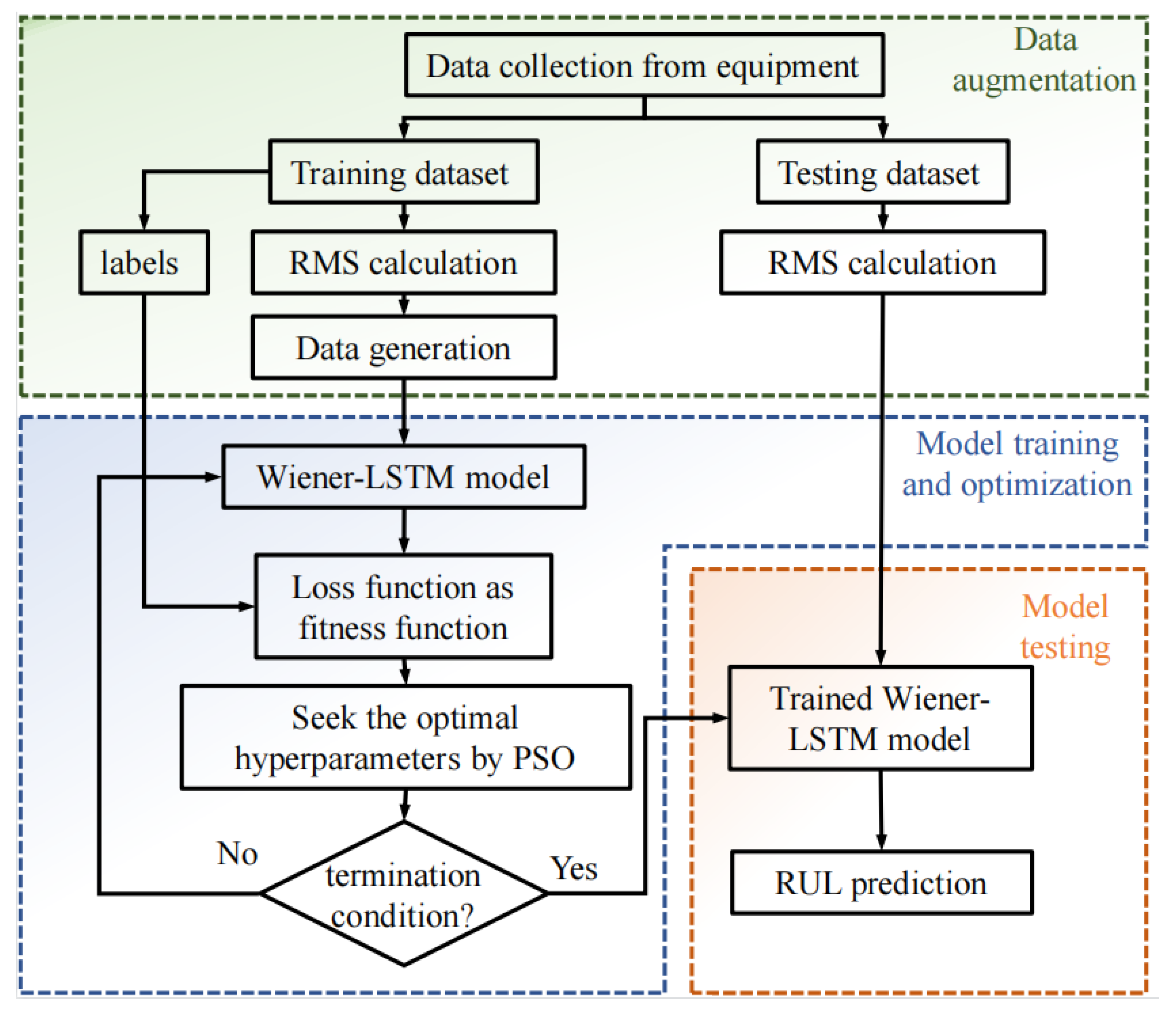
Figure 1 shows the proposed method’s structure, including two training and testing processes. In the training process, RMS of the vibration data is calculated firstly as the health indicator. Then, the Fault Occurrence Time (FOT) of each run-to-failure data is determined by the $3\sigma$ rule. RMS data of the degradation stage is prepared for the data augmentation. The data augmentation based on the degradation modeling and Sobol sampling are introduced in detail in Section 3.1. The run-to-failure data generated in the next step is used to train the Wiener–LSTM model. Then the PSO algorithm is applied to optimize the hyperparameters in the Wiener–LSTM model. The detailed descriptions of the Wiener–LSTM model are introduced in Section 3.2. In the testing process, the procedure is similar to the training process. The RMS of the testing datasets is calculated, and the FOT is determined by the $3\sigma$ rule. Then the testing datasets are sent to the trained Wiener–LSTM model to verify the effectiveness of the proposed method.

3.1. Data Augmentation Based on Degradation Modeling and Sobol Sampling

This study proposes a data generation method for producing enough data for training based on degradation modeling and Sobol sampling. The flowchart of the data generation method can be divided into four steps. Detailed descriptions of each step are given as follows.

(1)

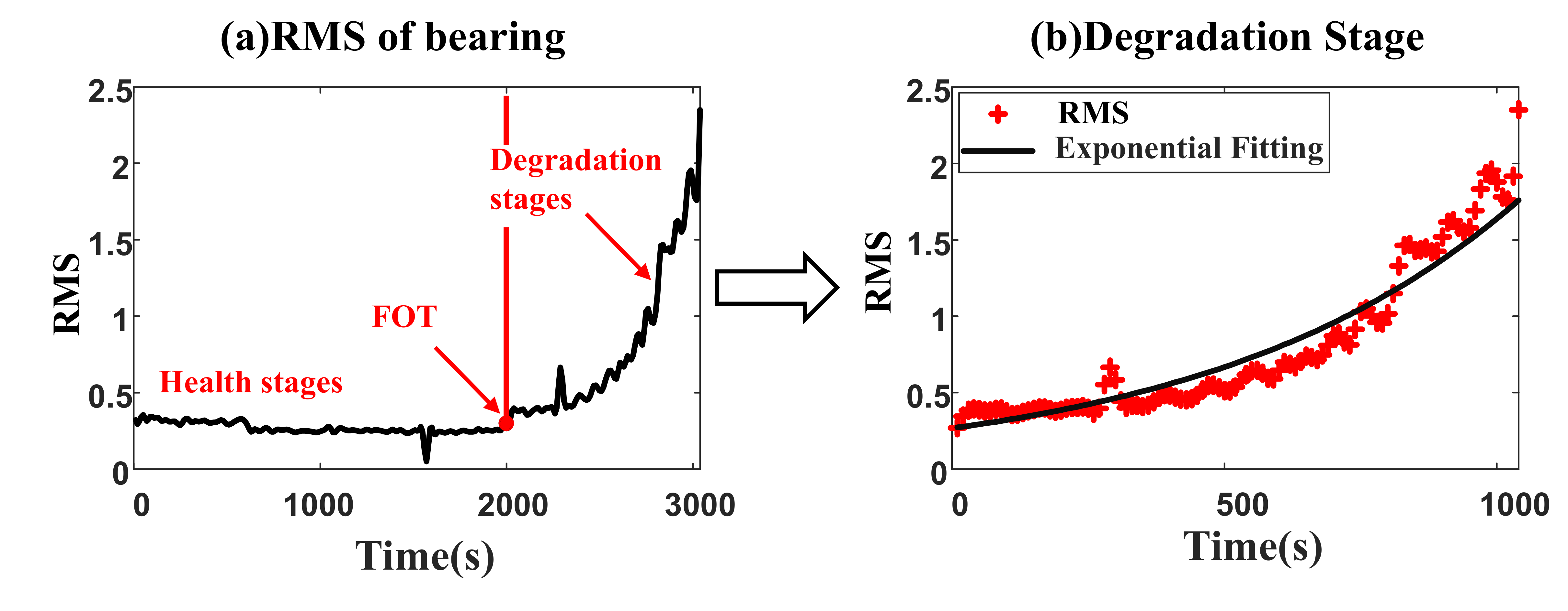
Degradation modeling is the first step. The RMS is a commonly used time-domain feature, which can reflect the degradation process. Thus, the RMS of the monitored bearing is chosen as the health indicator. The RMS of the whole life bearing signal is shown in Figure 2a, which can be divided into two different stages [36]. The bearing is in the health stage at an early time. RUL prediction is not necessary for this stage because RMS value in the health stage shows a smooth trend. At the Fault Occurrence Time (FOT), the bearing gets into the degradation stage. The degradation can be modeled as

$$X_t=\left\{\begin{array}{cc}exp(m+{\sigma }_1\epsilon \left(t\right))\hfill & t⩽\gamma \hfill \\ aexp(-\frac{e^2}{2}+b(t-\gamma )+e\epsilon (t-\gamma ))\hfill & t>\gamma \hfill \end{array}\right.,$$

(6)

where the $\gamma$ is the FOT, it is a random variable because different bearing has different FOT. When $t⩽\gamma$, the bearing is in the healthy stage. The m is a normal random variable representing a stable level of normal bearing health. The ${\sigma }_1$ is a noise variance in this healthy stage. $\epsilon \left(1\right)$, $\epsilon \left(2\right)\dots \dots$ in $\epsilon \left(t\right)$ is independent at different time. RUL prediction often starts from FOT to the failure time, which means the stage $t>\gamma$ is always used for RUL prediction. At this stage, a is a log-normal random variable representing the magnitude of the exponential degradation trend. b is a normal random variable representing the slope of the exponentially degenerate trend. e is the noise variance in the degradation process. If there are N number of vibration signal data at each sampling point as $D=[d_1,d_2,d_3,\dots ,d_N]$. In [37], commonly used health indicators in residual useful life prediction are root mean square (RMS), kurtosis, peak value, and so on. The RMS is a commonly used indicator to describe the degradation trends of bearings, due to its ability to reflect the vibration energy characteristics with robustness. In [38], it is also stated that the RMS indicator is a commonly used indicator in the machinery fault diagnosis and remaining useful life prediction. The RMS is chosen as the indicator in the proposed method, and the unit of RMS is ‘g’. The RMS of the vibration signal is calculated firstly as the health indicator as

$$x_i^{rms}=\sqrt{\frac{1}{N}\sum _{i=1}^N{\left(d_i-d_m\right)}^2},$$

(7)

where $d_i$ is the signal in the sampling point. $d_m$ is the mean of the signal recorded from 0–N. The FOT of the RMS is then calculated using the laida criterion, also known as the 3$\sigma$ rules. The RMS health stage mean $\mu$ and standard deviation $\sigma$ are calculated. The first value, which exceeds 3 $\sigma$ is assumed as the FOT. Then the data from FOT to failure are collected and prepared for the next step.

(2)

Since the RUL prediction is not necessary for the stage $t⩽\gamma$. The model fitting is implemented only in the stage $t>\gamma$ to acquire the parameters a, b, and e in Equation (6). The $\epsilon \left(t\right)$ follows a normal distribution, which can not be fitted in this process. All the training samples are fitted by the function of the degradation model. Different parameters are acquired after fitting different samples. If there are M run-to-failure data, M sets of parameters of $a,b,$ and e can be acquired after the model fitting on the M run-to-failure datasets. Among these sets of parameters, the maximum and minimum values should be chosen. Ranges of each parameter can be recorded as $[a_{min},a_{max}]$, $[b_{min},b_{max}]$ and $[e_{min},e_{max}]$.

(3)

The Sobol sequence sampling is used to get different combinations of parameters. Random sampling algorithms are quasi-random and limited to one period. When the cycle is exceeded the period, they are repeated and are no longer mutually independent random numbers. Sobol sequences sampling method focus on producing uniform distributions in the probability space compared with the random sampling method. Localized clustering can be avoided in this way. As one of the low deviation sequences, Sobol sequence sampling is superior to other low deviation sequences. The random numbers generated afterward will be distributed to the areas that were not previously sampled. A set of independent parameters can be acquired after one Sobol sequence sampling among the ranges of $[a_{min},a_{max}]$, $[b_{min},b_{max}]$ and $[e_{min},e_{max}]$. The algorithm of Sobol sequence sampling is as follows.

Consider i random data $Z_i$ are generated in the range of $[a_{min},a_{max}]$. $Z_i$ follows the normal distribution. A non-integrable polynomial $f\left(Z\right)$ can be constructed as

$$f\left(Z\right)=Z^n+m_1{Z}^{n-1}+m_2{Z}^{n-2}+\dots \dots +m_{n-1}Z+1,$$

(8)

where the n is the highest order. The $m_1,m_2,m_2,\dots \dots$ is the coefficients of the polynomial. The direction value $v_i$ can be acquired as

$$v_i=m_1{v}_{i-1}\oplus m_2{v}_{i-2}\oplus \cdots \oplus m_s{v}_{i-n}\oplus ⌊\frac{v_{i-n}}{2^n}⌋,$$

(9)

where the ⊕ is binary logic operation. ⌊⌋ is the rounding down operation. The random data $Z_i$ can be based on the direction value as

$$Z_i=b_1{v}_1\oplus b_2{v}_2\oplus b_3{v}_3\oplus \cdots b_i{v}_i,$$

(10)

where the $b_1,b_2,b_3,\dots \dots$ is the binary representation of i. After the Sobol sequence sampling operation is implemented on the ranges of parameters $a,b$, and e. i sets of parameters of the degradation model can be acquired.

(4)

Now, i sets of parameters sampled in the last step are substitute to the degradation model function in Equation 6 again without $\epsilon \left(t\right)$ to get i new run-to-failure data as

$$X_t^i=aexp(-\frac{e^2}{2}+b(t-\gamma )),$$

(11)

the rand noise $\epsilon (t-\gamma )$ is added in the new sample to imitate the random shock in the working situation in the last step. The i run-to-failure data are prepared and can be sent to the Wiener–LSTM model for the training process.

Figure 2. (a) The RMS of the whole life data of bearing (b) Degradation model fitting of the degradation stage. Two stages are included in the run-to-failure data of bearing. The RMS of the bearing shows a steady state in the health stage. After Failure Occurrence Time (FOT), the RMS of the bearing shows an exponential degradation in the degradation stages.

Figure 2. (a) The RMS of the whole life data of bearing (b) Degradation model fitting of the degradation stage. Two stages are included in the run-to-failure data of bearing. The RMS of the bearing shows a steady state in the health stage. After Failure Occurrence Time (FOT), the RMS of the bearing shows an exponential degradation in the degradation stages.

3.2. Wiener–LSTM Bearing RUL Prediction Model

3.2.1. Forward Propagation of the LSTM $\varphi$

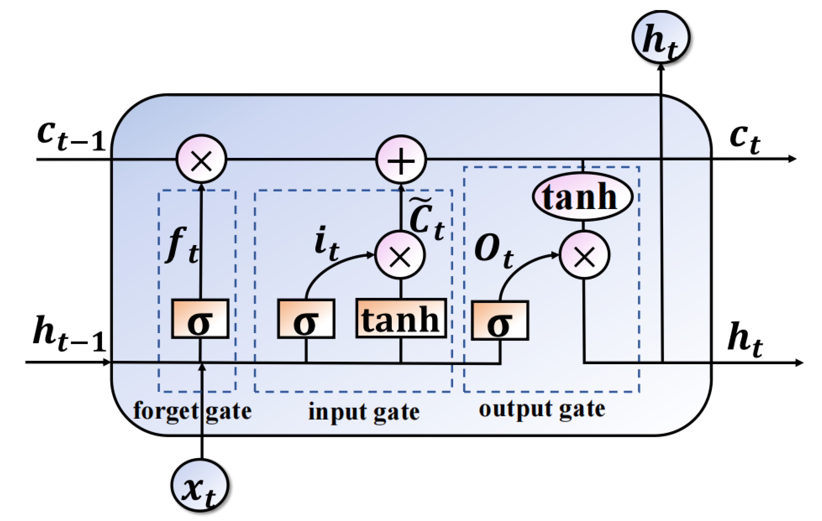
The LSTM network is established as the RUL predictor in the proposed method, which is one of the variants of the Recurrent Convolutional Neural (RNN). The gradient vanishing and explosion problems of the RNN can be addressed by the LSTM network memory cell. Figure 3 shows the memory neuron structure of the LSTM network. The memory neuron consists of three kinds of gate units called forget gate $f_t$, input gate $i_t$, and output gate $O_t$. The forward propagation process of the automatic predictor $\varphi$ is introduced in detail now.

The forget gate is used to determine what information should be discarded. The input of the forget gate is the output of the hidden state in last time $h_{t-1}$ and the current time input data $x_t$. The $x_t$ is the signal of the monitored machine at time t. The important information of the last time would be reserved and the redundant information would be discarded. The calculation process of the forget gate can be followed as

$$f_t=\sigma \left(W_f·h_{t-1}+W_f·x_t+b_f\right),$$

(12)

where $W_f$ and $b_f$ are the weights and bias of forget gate. $\sigma$(·) is the sigmoid activation function.

Two steps are involved in this part. The first step is the calculation of the input gate. The second step is adding the candidate values ${\tilde{C}}_t$ to the memory cell $C_t$. $C_{t-1}$ is the old state value of the memory cell at time $t-1$, $C_t$ is the new state value of cell at time t which is updated by the process as

$$\begin{array}{c}{i}_t=\sigma \left(W_i·h_{t-1}+W_i·x_t+b_i\right),\hfill \\ {\tilde{C}}_t=tanh\left(W_i·h_{t-1}+W_i·x_t+b_C\right),\hfill \\ C_t=f_t\ast C_{t-1}+i_t\ast {\tilde{C}}_t,\hfill \end{array}$$

(13)

where $W_i$ and $b_i$ are the weights and bias of input gate. $i_t$ is the output of the input gate. * denotes dot product.

The output gate is used to determine what information should be exported as

$$\begin{array}{c}{O}_t=\sigma \left(W_O·h_{t-1}+W_O·x_t+b_O\right),\hfill \\ h_t=O_t\ast tanh\left(C_t\right),\hfill \end{array}$$

(14)

where $W_O$ and $b_O$ are the weights and bias of the output gate. $h_t$ denotes the output of the LSTM cell at time t. The LSTM layer is normally constructed with the dense layer, the output $h_t$ of the LSTM is the input of the dense layer. The output of the dense layer is the predicted RUL, which can be calculated as

$${\alpha }_t=\sigma \left(W_d·h_t\left(x_t\right)+b_d\right),$$

(15)

where $W_d$ and $b_d$ are the weights and bias of the dense layer. All the parameters of the LSTM layer and dense layer, such as $W_f$, $b_f$, $W_i$, $b_i$, and so on, are recorded as $\Theta$ for convenience.

3.2.2. The Wiener–LSTM Model with Joint Optimization Loss Function

In order to control the uncertainty of the increment of the prediction result, the uncertainty of the predicted RUL is modeled by the Wiener process. The object of the training of the LSTM network is shown in Equation (5) now. The possibility function of $r_t$, ${\alpha }_t$, and ${\alpha }_s$ should be acquired to solve the parameters in Equation (5) The possibility of joint prediction for two times is recorded as $P(r_t,{\alpha }_t,{\alpha }_s)$. The joint equations can be get to solve the possibility of joint prediction as

$$\left\{\begin{array}{c}\varphi \left({\mathbf{x}}_{0:t};\Theta \right)={\alpha }_t\hfill \\ \varphi \left({\mathbf{x}}_{0:s};\Theta \right)={\alpha }_s\hfill \\ P(r_t,{\alpha }_t,{\alpha }_s)=P\left({\alpha }_s\right)P({\alpha }_t\mid r_s)P(r_t\mid {\alpha }_t),\hfill \end{array}\right.$$

(16)

where the ${\alpha }_t$ and ${\alpha }_s$ at different times are dependent because of the Markov property of the stochastic process. The possibility of the joint prediction $P(r_t,{\alpha }_t,{\alpha }_s)$ can be transformed as three possibility as shown in Equation (16). $r_t$ denotes the real RUL at time t, the ${\alpha }_t$, and ${\alpha }_s$ denotes the RUL predicted by the predictor at time t and s ($t>s$).

The modeling of $P({\alpha }_t\mid {\alpha }_s)$, $P(r_t\mid {\alpha }_t)$ and $P\left({\alpha }_s\right)$ is given in [35] As for two predicted RUL ${\alpha }_t$ and ${\alpha }_s$ at two times $t>s$, the prediction increment is assumed to follow the normal distribution

$${\alpha }_t-{\alpha }_s\sim \mathcal{N}(s-t,(t-s)/c),$$

(17)

where the mean of the normal distribution is $s-t$, the variance of the normal distribution is $(t-s)/c$. The $P\left({\alpha }_s\right)$ is assumed to follow the normal distribution [35]

$${\alpha }_s\sim \mathcal{N}\left(r_s,r_s/c\right).$$

(18)

The $P(r_t\mid {\alpha }_t)$ follows the Inverse Gaussian distribution [39]

$$IG({\alpha }_s,c)={\left[\frac{c{\alpha }_s^2}{2\pi x^3}\right]}^{1/2}exp\left\{\frac{-c{(x-{\alpha }_s)}^2}{2x}\right\},$$

(19)

where $IG$ denotes the Inverse Gaussian distribution. The means of the distribution is ${\alpha }_s$, the variance of the distributed is ${\alpha }_s/c$.

Thus, inspired by the joint likelihood possibility proposed in Equation (16), the loss function is reconstructed to guide the uncertainty control and accuracy improvement. As for a run-to-failure sample, the failure time of the machine is recorded as $\tau$. ${\alpha }_0,{\alpha }_1,{\alpha }_2\dots \dots$ denotes the predicted RUL at different times. If the historical predictions are all considered in the joint likelihood possibility function, which can be represented as

$$\left\{\begin{array}{c}\varphi \left({\mathbf{x}}_0;\Theta \right)={\alpha }_0\hfill \\ \varphi \left({\mathbf{x}}_{0:1};\Theta \right)={\alpha }_1\hfill \\ \dots \dots \hfill \\ \varphi \left({\mathbf{x}}_{0:\tau };\Theta \right)={\alpha }_{\tau }\hfill \\ P(r_{\tau },{\alpha }_{\tau },{\alpha }_{\tau -1}\dots {\alpha }_0)=P\left({\alpha }_0\right)\prod _{i=1}^{\tau }P({\alpha }_i\mid {\alpha }_{i-1})P(r_{\tau }\mid {\alpha }_{\tau }).\hfill \end{array}\right.$$

(20)

All the samples should be considered in the joint likelihood function as the new loss function of the Wiener–LSTM network. Then the joint likelihood function can be maximized automatically by several iterations of the LSTM network. The new loss function can be expressed as

$$\begin{array}{c}\hfill Los{s}_{new}({\mathbf{x}}_{0:\tau }^n,{\mathbf{r}}_{0:t}^n;\Theta ,c)=-\frac{2}{N}{\displaystyle \sum _{n=1}^N}\left(P\left({\alpha }_0^n\right){\displaystyle \prod _{i=1}^{\tau }}P({\alpha }_i^n\mid {\alpha }_{i-1}^n)P(r_{\tau }^n\mid {\alpha }_{\tau }^n)\right),\end{array}$$

(21)

where n denotes the number of the running-to-failure samples.

The parameters of the LSTM network include $\Theta$ and c now. $\Theta$ are the parameters of the LSTM network. c is the parameter of the Wiener process which can control the uncertainty of the predicted RUL. However, the parameter c cannot be updated by the iteration of the LSTM network. It is a parameter out of the structure of the LSTM network. The c and the $\Theta$ can not be updated simultaneously by the iteration of the LSTM network. Therefore, the optimal value of c should be calculated first. The variable $\Theta$ is assumed as the constant value in the process of solving the optimal valve c

$$c^{*}=\frac{n+1}{{\sum }_{n=1}^N\left[\frac{{\left(r_{\tau }^n-{\varphi }^n({\mathbf{x}}_{0:\tau };\Theta )\right)}^2}{r_{\tau }^n}+\frac{{\left(r_0^n-{\varphi }^n(x_0;\Theta )\right)}^2}{r_0^n}+{\sum }_{i=1}^{\tau }{\left({\varphi }^n({\mathbf{x}}_{0:i};\Theta )-{\varphi }^n({\mathbf{x}}_{0:i-1};\Theta )+1\right)}^2\right]}.$$

(22)

The optimal $c^{*}$ can be expressed only including parameter $\Theta$ now. The expression of the parameter $c^{*}$ can be substituted into the new loss function. All the parameters of the loss function can be updated by iteration of the LSTM network. The proposed loss function of the LSTM network is the logarithmic function as

$$\begin{array}{cc}log\left({Loss}_{new}\left({\mathbf{x}}_{0:\tau }^n,{\mathbf{r}}_{0:\tau }^n;\Theta \right)\right)=\hfill & \frac{1}{N}{\displaystyle \sum _{n=1}^N}\left\{3log\left(2\pi \right)-log\left(c^{*}\right)+log\left(r_0^n\right)+\frac{c^{*}{\left(r_0^n-{\varphi }^n\left(x_0,r_0;\Theta \right)\right)}^2}{r_0^i}+\right.\hfill \\ & +c^{*}{\displaystyle \sum _{i=1}^{\tau }}{\left({\varphi }^n\left({\mathbf{x}}_{0:i},{\mathbf{r}}_{0:i};\Theta \right)-{\varphi }^n\left({\mathbf{x}}_{0:i-1},{\mathbf{r}}_{0:i-1};\Theta \right)+1\right)}^2+\hfill \\ & \left.-2log\left({\varphi }^n\left({\mathbf{x}}_{0:\tau },{\mathbf{r}}_{0:\tau };\Theta \right)\right)+3log\left(r_{\tau }^n\right)+\frac{c^{*}{\left(r_{\tau }^n-{\varphi }^n\left({\mathbf{x}}_{0:\tau },{\mathbf{r}}_{0:\tau };\Theta \right)\right)}^2}{r_{\tau }^n}\right\}\hfill \end{array}$$

(23)

The log-likelihood loss function, as shown in Equation (23) is convenient for calculating. The new loss function is the training object of the Wiener–LSTM model. During backpropagation, the parameter $\Theta$ is updated using the Adam algorithm. The Adam algorithm is a first-order optimization technique that, like a conventional stochastic gradient descent procedure, iteratively adjusts the weights of the neural network based on training data [40]. The process ${\Theta }^{*}=arg{min}_{\Theta }Los{s}_{new}({\mathbf{x}}_{0:\tau }^n,{\mathbf{r}}_{0:\tau }^n;\Theta )$ can be acquired by the Adam algorithm.

3.2.3. Optimization of the Hyperparameters by PSO Algorithm

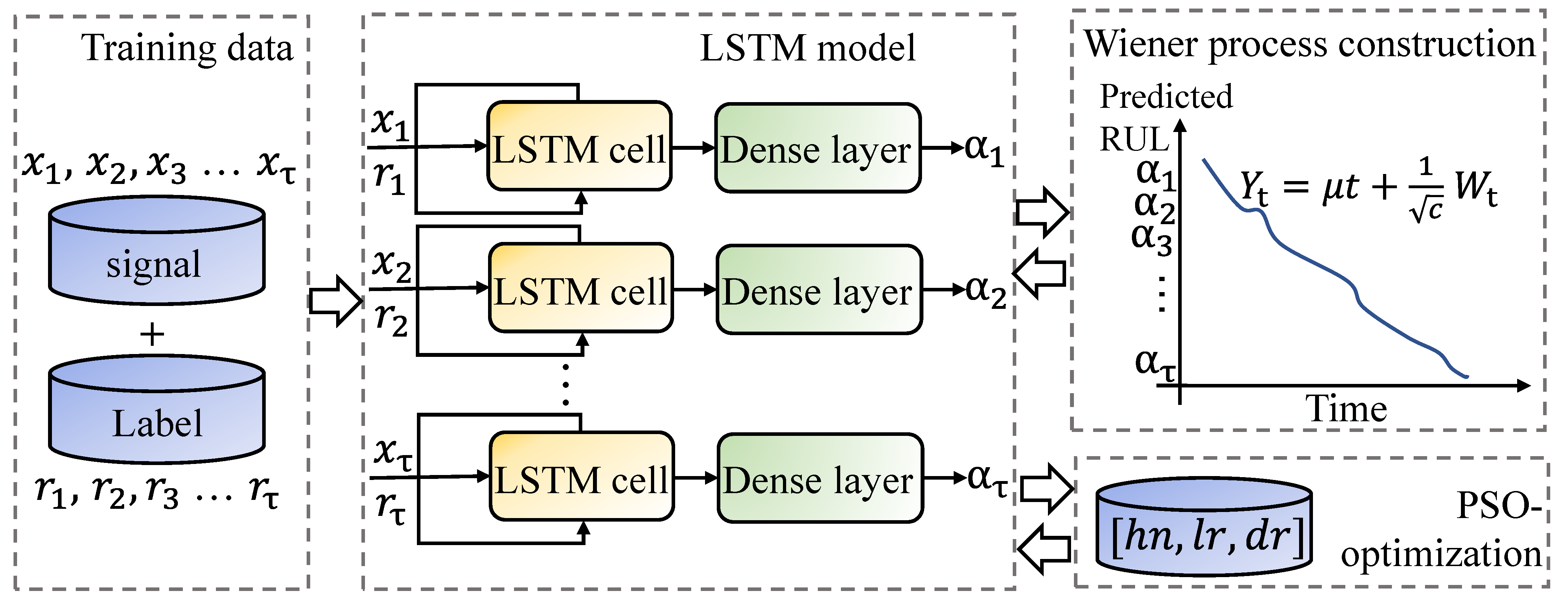
It is well known that the performance of the network is influenced by the hyperparameters, such as the learning rate, number of neurons, maximum epochs, and so on. However, these hyperparameters are always tested by so many trials to seek the optimal structure of the network. As one of the optimization algorithms, the PSO algorithm has been widely used in several optimization tasks of the network [41] because of the fast convergence and robust applicability. The structure of the Wiener–LSTM model with PSO optimization is shown in Figure 4. The Wiener–LSTM model consists of one LSTM layer and one dense layer. Thus, the hyperparameters in this model include the number of hidden layer neurons ($hn$), initial learning rate ($lr$), and drop rate factor ($dr$). The process of the optimization can be divided into four steps:

• Step 1: Parameter initialization. The particle dimension, population size, iterations, learning factors, inertia weight, velocity, and position are determined.
• Step 2: Initialize the particle positions and velocities, then generate population particle ($hn,lr,dr$) at random.
• Step 3: The loss function in Equation (23) is chosen to be the fitness function in the PSO algorithm here. The particle position and velocity are updated by epoch. The extreme individual value and extreme global value are then updated by computing the fitness value in accordance with the new situation.
• Step 4: Judge whether the termination conditions are met. If satisfied, the algorithm ends and outputs the optimization result ($hn,lr,dr$); otherwise, return to Step 1.

Figure 4. The structure of the Wiener–LSTM model with PSO optimization. The signals measured by sensors are $x_1,x_2,x_3,\dots x_t$ at time $1,2,3,\dots t$. The corresponding RUL is recorded as $r_1,r_2,r_3,\dots r_t$. The predicted RUL ${\alpha }_1,{\alpha }_2,{\alpha }_3,\dots {\alpha }_t$ is predicted by the LSTM network ($\varphi$). The Wiener process $Y_t$ of the predicted RUL is introduced to control the uncertainty of the predicted result. $W_t$ denotes the standard Wiener process. c is the parameter used to control the uncertainty propagation rate. The Wiener process can be introduced into LSTM in the back propagation of the LSTM network.

Figure 4. The structure of the Wiener–LSTM model with PSO optimization. The signals measured by sensors are $x_1,x_2,x_3,\dots x_t$ at time $1,2,3,\dots t$. The corresponding RUL is recorded as $r_1,r_2,r_3,\dots r_t$. The predicted RUL ${\alpha }_1,{\alpha }_2,{\alpha }_3,\dots {\alpha }_t$ is predicted by the LSTM network ($\varphi$). The Wiener process $Y_t$ of the predicted RUL is introduced to control the uncertainty of the predicted result. $W_t$ denotes the standard Wiener process. c is the parameter used to control the uncertainty propagation rate. The Wiener process can be introduced into LSTM in the back propagation of the LSTM network.

4. Experiment

This paper uses a popular dataset to verify the effectiveness of the proposed Wiener–LSTM network. All code was run on a PC with an Intel Core i7-5557U CPU, and 4 GB RAM. The codes are based on the Keras framework using the Tensorflow backend.

4.1. Data Description

In Figure 5, the accelerated degradation experiments are taken in the PRONOSTIA platform [42]. Three parts, such as the rotating part, the degradation part, and the measurement part, are included in the platform. The degradation part is used to accelerate the bearing degradation. This platform of the PHM2012 dataset is composed of two high-frequency accelerometers of type 3035B DYTRAN placed horizontally and vertically on each bearing to pick up the horizontal and vertical vibration signals. The accelerometer is a single axis with a range of 50 g, and the response frequency is 0.34 to 10,000 Hz. Two acceleration sensors are mounted on the vertical and horizontal axes in order to measure the bearing’s vibration signal. Compared to the vertical vibration signal, the horizontal vibration signal has a higher and more noticeable amplitude. As a result, the experiment solely uses the horizontal vibration signal. The sampling frequency is 25.6 kHz, and the signal is sampled for 0.1 s every 10 s. The experiments contain 17 run-to-failure bearings. All the datasets are shown in

Table 1. Datasets of IEEE PHM 2012 prognostic challenge.

Data Set	Operation Conditions
	Conditions 1	Conditions 2	Conditions 3
Load (N)	4000	4200	5000
Speed (rpm)	4800	1650	1500
Training set	Bearing 1$\_$1	Bearing 2$\_$1	Bearing 3$\_$1
	Bearing 1$\_$2	Bearing 2$\_$2	Bearing 3$\_$2
Testing set	Bearing 1$\_$3	Bearing 2$\_$3	Bearing 3$\_$3
	Bearing 1$\_$4	Bearing 2$\_$4
	Bearing 1$\_$5	Bearing 2$\_$5
	Bearing 1$\_$6	Bearing 2$\_$6
	Bearing 1$\_$7	Bearing 2$\_$7

. The raw vibration acceleration signal of the test bearing1_3 is shown in Figure 6. The signal to the left of FOT is the healthy bearing signal, and the one to the right of FOT is the fault signal. The overall time domain waveform shows that the vibration acceleration amplitude is relatively low in the front, starts to gradually increase after the early failure point FOT, and increases dramatically after the failure stage. The lower left figure shows the signal in the normal phase, with lower amplitude and a smoother signal. The lower right figure shows the signal in the failure phase, and the vibration amplitude is larger than the normal state, which can be seen due to the shock component caused by the failure.

4.2. Data Generation Based on the Degradation Model and Sobol Sampling

Five run-to-failure training data are used to fit the degradation model here. Bearing3_1 is discarded because the RMS of this bearing is not suitable for the degradation model in Equation (6). Then five sets of parameters $a,b,e$ can be acquired by the proposed data augmentation method. 250 run-to-failure data are generated for the preparation of the Wiener–LSTM training. Ten examples of the generated run-to-failure data are shown in Figure 7. The lifetime of the generated run-to-failure data ranges from 1000 s to 3000 s. It should be noted that the RUL of the bearing is calculated from the Failure Occurrence Time (FOT), while the PHM2012 is an accelerated degradation experiment.

In Figure 7, the number $1,2,3,\dots \dots ,10$ denotes the generated run to failure data of bearing 1 to 10. The horizontal axis shows the inspection time. The vertical l axis shows the value of RMS. The RMS of the generated run to failure bearing data is consistent with the exponential model. To simulate the run to failure data with a different lifetime, the generated data are different from each other.

As for the testing data. Bearing 1_3 and Bearing 1_4 are chosen to verify the effectiveness of the proposed method. The RMS values of the Bearing 1_3 and Bearing 1_4 are calculated and the data of 1000 s before failure are used for RUL prediction on these two testing bearings.

4.3. Wiener–LSTM Training and Optimization

A Wiener–LSTM model with PSO optimization is proposed to control the uncertainty and improve the accuracy of the prediction RUL simultaneously. In the training process, the time-domain feature RMS of the vibration signal is calculated first. Then, the data are generated according to the data augmentation model for model training. In the testing process, the RMS of the testing vibration signal is sent to the predictor which has trained in the training process. Then, the predicted RUL of the testing data can be given by the predictor automatically. The prediction uncertainty model of the predicted RUL is introduced in the LSTM network. When the loss function (introduced in Equation (23)) is used in the LSTM model. The training sample of the Wiener–LSTM should be a sequence of data such as $x_{0:t}$, which is different from the point prediction that one training sample is one data at time t. Thus, the relationship of the difference of predicted RUL ${\alpha }_{t+1}-{\alpha }_t,{\alpha }_t-{\alpha }_{t-1}\dots \dots$ can be established and introduced in the LSTM model.

A randomly under-sample method based on mini-batch is implemented in the training process, which is different from the normal LSTM training process with the same training sample in every epoch. Fixed-length sub-sequence from every input sequence is used to form a data batch. The fixed length of the sub-sequence is set for the minimum of the length of the input sequences. The under-sampling method in each minibatch can guarantee the independence of the statistical process and make full use of each sequence of data. The fixed length of the sub-sequence is set for 99 (to make full use of each sequence data among under-sample, the fixed-length equals the minimum value of the lifetime data minus one). The process of the under-sample method based on mini-batch follows three steps: (1) under-sampling method is implemented to get the training sample $X_i$; (2) c value is updated by Equation (22); and (3) parameters $\Theta$ are updated by the Adam algorithms. The algorithm of the under-sample method based on mini-batch is in Algorithm 1.

Algorithm 1: Down-sample algorithm based on mini-batch

Input: Training data X, corresponding RUL r, epoch of training process I

1: initialization $\Theta$ and c of the network.

2: If i < I

3:   $X_i$ are under-sampled on training data X.

4:   Update parameter c by Equation (22)

5:   Update parameter $\Theta$ by random gradient descent algorithm by the loss function in Equation (23)

6: End

7: return (${\Theta }^{*}$, $c^{*}$)=argmin(log(loss($\Theta$, c, X))).

Output:${\Theta }^{*}$, $c^{*}$

The structure of the LSTM model contains two layers: one LSTM layer and one fully-connected layer. After the optimization by the PSO algorithm, the optimal number of neurons in LSTM is set for 64. The optimal dropout rate is 0.23, and the optimal learning rate is 0.02; the activation function is ReLU. In the fully-connected layer, the number of neurons is set for 1, and the activation function is sigmoid. The input of the Wiener–LSTM model is (250, 99, 1). The number of the training sample is 250, the length of each sub-sequence under-sampled in each epoch is 99, and the feature of input data is 1. The label of the training data is (250, 99), which is the corresponding RUL of training samples.

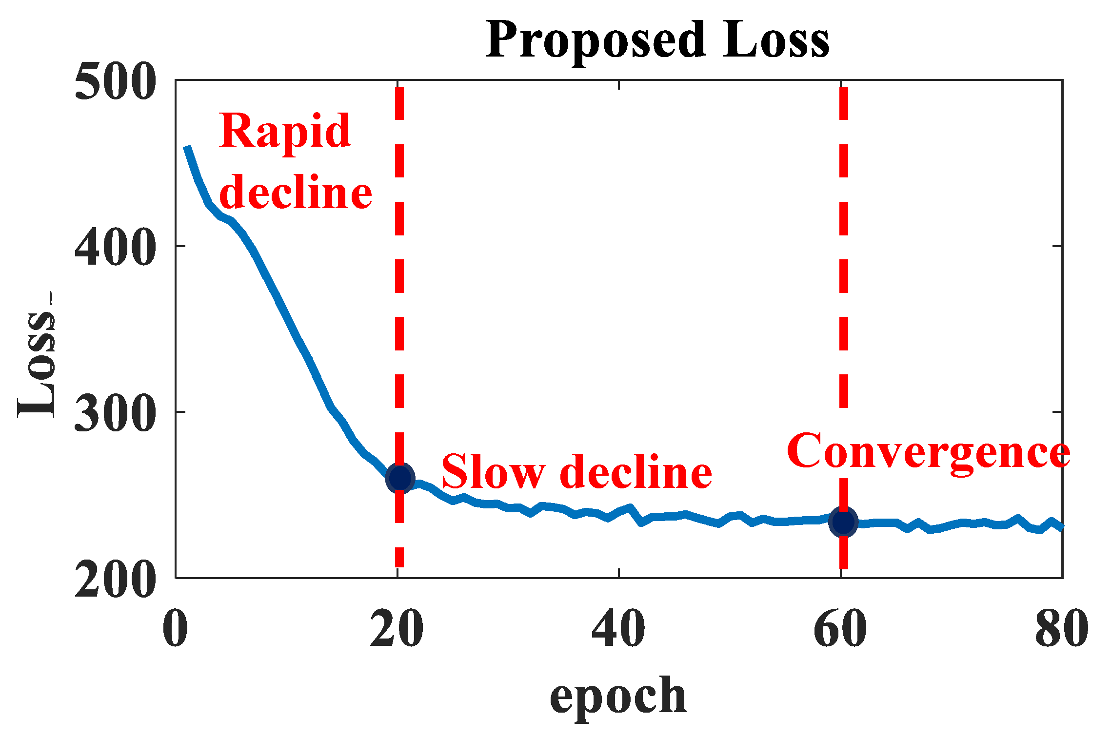
The loss functions of Wiener–LSTM model among epochs are shown in Figure 8. The X-axis represents the number of epoch. The Y-axis represents the magnitude of the loss function. As shown in Figure 8 from the first to the 20th epoch, the Wiener–LSTM model’s training loss function dramatically decreased. From the 20th to the 60th epoch, the loss function continues slowly degrade. The loss function gradually finds convergence from the 60th to the 80th epoch.

4.4. Results and Discussions

4.4.1. Comparison 1

To verify the effectiveness of the data augmentation strategy, the comparison experiments between the Wiener–LSTM model with data augmentation and without data augmentation are taken. The predicted RUL by 6 training samples without data augmentation on test bearing1_3 and bearing1_4 are shown in Figure 9. The blue line is the real RUL from time 1000–0 s. The orange line represents the outcome that the Wiener–LSTM model anticipated. In the training process, only six training samples are used to train the Wiener–LSTM model such as bearing1_1, bearing1_2, bearing2_1, bearing2_2, bearing3_1, bearing3_2. The result of the test bearing1_3 is shown in Figure 9a. The result of the test bearing1_4 is shown in Figure 9b. The predicted RUL are far from the real RUL in the Figure 9 both in test bearing1_3 and test bearing1_4. Thus, enough training samples are necessary for the training process of the Wiener–LSTM model.

4.4.2. Comparison 2

To verify the effectiveness of the Wiener–LSTM model, the comparison experiments between the Wiener–LSTM model and the LSTM model are taken. In the training process of the LSTM model, the loss function MSE is shown in Figure 10. The training loss function of normal MSE declines rapidly from the beginning to the 10th epoch and shows a steady trend from the 10th epoch to the 80th epoch. The results of the loss function curve show that each model has reached convergence at the 80th epoch. The same number of epoch should be ensured for the two models for comparison. Thus the training epoch is set for 80.

Predicted RUL results by Wiener–LSTM and LSTM models are shown in Figure 11. The blue line in Figure 11a,b represents the real RUL of the bearing1_3 and bearing1_4. The orange line is the result predicted by the Wiener–LSTM model with the loss function in Equation (23). The yellow line indicates the result predicted by the normal LSTM using the MSE loss function. Both models have the same structure: the same layers and the same number of neurons in each layer. Predicted results of the test bearing1_3 are shown in Figure 11a. As for the test bearing1_3, the curve of the predicted RUL based on the Wiener–LSTM model is closer to the real RUL than the results based on the normal LSTM model at the beginning 0–400 s. After 400 s, the predicted RUL based on the Wiener–LSTM model is farther from the real RUL than the results based on the normal LSTM model. Although the Wiener–LSTM model has worse accuracy than the normal LSTM model at the end of the time in Figure 11. The predicted result based on the Wiener–LSTM model has a stable result without large fluctuation. On the contrary, the unstable RUL result with fluctuations is predicted by the LSTM model. The large fluctuation of the predicted RUL would affect the decision-making of the maintain. However, the predicted RUL results by the Wiener–LSTM model are smooth. The assumed Wiener process is proved that can be well fitted by the LSTM model to control the uncertainty of the predicted RUL. The uncertainty of the RUL between continuous time can be controlled by the Wiener–LSTM model. The predicted result based on Wiener–LSTM shows better accuracy than the LSTM model for test bearing1_4 as shown in Figure 11b. The predicted RUL curve is closer to the real RUL (the blue line) than the LSTM model all the time. The curve of the RUL result predicted by the Wiener–LSTM model is smoother than the RUL result predicted by the LSTM model. Fluctuations are obvious in the result of the LSTM model. The uncertainty of the result can be well controlled no matter which test bearing. The reliability of maintenance decisions is improved by the proposed Wiener–LSTM model.

A normal indicators Mean Absolute Error (MAE) is implemented in this paper to assess the predicted result quantitatively. The functions of the MAE is

$$MAE=\sum _{i=1}^N\left|r_i-{\alpha }_i\right|/N,$$

(24)

where the $r_i$ denotes the real RUL at time i, the ${\alpha }_i$ denotes the predicted RUL at time i. N is the number of the samples.

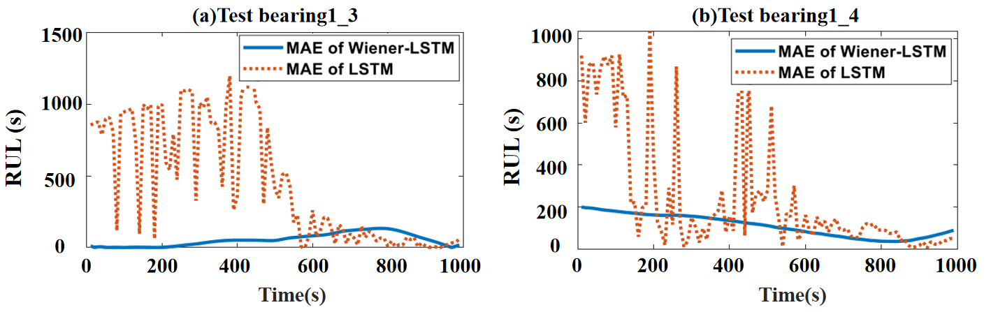
The MAE of the predicted results by Wiener–LSTM and LSTM models are shown shown in Figure 12. The MAE of the predicted results of the test bearing1_3 is shown in Figure 12a. The MAE of the predicted results of the test bearing1_4 is shown in Figure 12b. The blue line is the MAE result by using the Wiener–LSTM model. The orange line is the MAE result by using the LSTM model. In Figure 12a, The MAE of the Wiener–LSTM model is lower than the LSTM model on the test bearing1_3 at the beginning time 0–600 s. Although the MAE of the LSTM model is mostly the same as the Wiener–LSTM model. The MAE of the LSTM model has large fluctuation. On the contrary, the MAE of the Wiener–LSTM model is smooth all the time. The prediction uncertainty of the result can be proved that controlled by the Wiener–LSTM model in Figure 12. The error of the predicted result is in a stable state, which means the uncertainty of the predicted result is in a stable state without large fluctuations. It is important for the maintenance decisions in the industry. The MAE of the Wiener–LSTM model is lower than the LSTM model on bearing 1_4, as shown in Figure 12b, and it is more smooth than the LSTM model. As shown in

Table 2. Numerical prognostic performance comparisons of different methods.

	Proposed	LSTM
Test Bearing	MAE	MAE
Bearing1_3	6.34	43.6
Bearing1_4	8.03	23.8

, the proposed method is applied to the test bearing1_3 and bearing1_4 data. The MAE error between the remaining useful life predicted by the proposed method and the true remaining useful life is much lower than that of the traditional LSTM method. The larger MAE error in the testing process indicates a lower accuracy of the model, and conversely, a minor MAE error indicates a higher accuracy. It is evident that the uncertainty of the result can be well controlled by the Wiener–LSTM model by the experiments on the test bearing1_3 and bearing1_4. The large fluctuations can be removed from the RUL prediction by using the proposed Wiener–LSTM model.

5. Conclusions

In this paper, a bearing RUL prediction method with data augmentation strategy and Wiener–LSTM network with PSO optimization is proposed. The data augmentation method is designed to offer enough training data for the training process. The Wiener–LSTM model is constructed to improve the accuracy of the predicted RUL and control the uncertainty of the result simultaneously. The difference in the predicted RUL result is modeled by the Wiener process to control the uncertainty propagation rate of the result. Wiener process is applied as the connection between the parametric probabilistic model and the LSTM model. The parameters in the Wiener process model and the LSTM network can be updated iteratively by optimizing the joint probability loss function. The proposed Wiener–LSTM method is verified on a popular dataset. The predicted RUL shows better accuracy on test bearings than the normal LSTM model, and the uncertainty of the RUL result can be proved well controlled in the experiments. The stable RUL results with fewer fluctuations predicted by the proposed Wiener–LSTM model are more suitable for decision-making in industrial applications. Two error metrics are applied to verify the validity of the proposed method. The larger MAE error in the testing process indicates a lower accuracy of the model, and conversely, a minor MAE error indicates a higher accuracy. On the test bearing1_3 and bearing1_4, the MAE error of the proposed method is 6.34 and 8.03, which is much lower than that of the traditional LSTM model. The PSO algorithm method is applied here to solve the problem of hyperparameter optimization. An uncertainty propagation modeling framework is proposed for automatic predictors, such as deep learning models. The great potential of the combination of the statistical model and the DL model has been shown in the experiments. Future research on interactive training between the surrogate model and the automatic RUL predictor should be proposed and realized.

References

- Ueda, M.; Wainwright, B.; Spikes, H.; Kadiric, A. The effect of friction on micropitting. Wear 2022, 488–489, 204130. [Google Scholar] [CrossRef]
- Ambrożkiewicz, B.; Syta, A.; Gassner, A.; Georgiadis, A.; Litak, G.; Meier, N. The influence of the radial internal clearance on the dynamic response of self-aligning ball bearings. Mech. Syst. Signal Process. 2022, 171, 108954. [Google Scholar] [CrossRef]
- Sahu, P.K. Grease Contamination Detection in the Rolling Element Bearing Using Deep Learning Technique. Int. J. Mech. Eng. Robot. 2022, 11, 275–280. [Google Scholar] [CrossRef]
- Xie, Z.; Jiao, J.; Yang, K.; He, T.; Chen, R.; Zhu, W. Experimental and numerical exploration on the nonlinear dynamic behaviors of a novel bearing lubricated by low viscosity lubricant. Mech. Syst. Signal Process. 2023, 182, 109349. [Google Scholar] [CrossRef]
- Lei, Y.; Li, N.; Guo, L.; Li, N.; Yan, T.; Lin, J. Machinery health prognostics: A systematic review from data acquisition to RUL prediction. Mech. Syst. Signal Process. 2018, 104, 799–834. [Google Scholar] [CrossRef]
- Zhu, J.; Chen, N.; Shen, C. A new data-driven transferable remaining useful life prediction approach for bearing under different working conditions. Mech. Syst. Signal Process. 2020, 139, 106602. [Google Scholar] [CrossRef]
- Zhang, Z.X.; Si, X.S.; Hu, C.; Lei, Y. Degradation Data Analysis and Remaining Useful Life Estimation: A Review on Wiener-Process-Based Methods. Eur. J. Oper. Res. 2018, 271, 775–796. [Google Scholar] [CrossRef]
- Liao, G.; Yin, H.; Chen, M.; Lin, Z. Remaining useful life prediction for multi-phase deteriorating process based on Wiener process. Reliab. Eng. Syst. Saf. 2021, 207, 107361. [Google Scholar] [CrossRef]
- Wang, H.; Liao, H.; Ma, X.; Bao, R. Remaining Useful Life Prediction and Optimal Maintenance Time Determination for a Single Unit Using Isotonic Regression and Gamma Process Model. Reliab. Eng. Syst. Saf. 2021, 210, 107504. [Google Scholar] [CrossRef]
- Lin, C.P.; Ling, M.H.; Cabrera, J.; Yang, F.; Yu, D.Y.W.; Tsui, K.L. Prognostics for lithium-ion batteries using a two-phase gamma degradation process model. Reliab. Eng. Syst. Saf. 2021, 214, 107797. [Google Scholar] [CrossRef]
- Du, W.; Hou, X.; Wang, H. Time-Varying Degradation Model for Remaining Useful Life Prediction of Rolling Bearings under Variable Rotational Speed. Appl. Sci. 2022, 12, 4044. [Google Scholar] [CrossRef]
- Song, K.; Cui, L. A common random effect induced bivariate gamma degradation process with application to remaining useful life prediction. Reliab. Eng. Syst. Saf. 2022, 219, 108200. [Google Scholar] [CrossRef]
- Peng, Y.; Wang, Y.; Zi, Y. Switching State-Space Degradation Model With Recursive Filter/Smoother for Prognostics of Remaining Useful Life. IEEE Trans. Ind. Inform. 2019, 15, 822–832. [Google Scholar] [CrossRef]
- Wang, Y.; Wu, J.; Cheng, Y.; Wang, J.; Hu, K. Memory-enhanced hybrid deep learning networks for remaining useful life prognostics of mechanical equipment. Measurement 2022, 187, 110354. [Google Scholar] [CrossRef]
- Wang, B.; Lei, Y.; Li, N.; Li, N. A Hybrid Prognostics Approach for Estimating Remaining Useful Life of Rolling Element Bearings. IEEE Trans. Reliab. 2020, 69, 401–412. [Google Scholar] [CrossRef]
- Soualhi, A. Bearing Health Monitoring Based on Hilbert–Huang Transform, Support Vector Machine, and Regression. IEEE Trans. Instrum. Meas. 2014, 64, 52–62. [Google Scholar] [CrossRef] [Green Version]
- Chelmiah, E.T.; McLoone, V.I.; Kavanagh, D.F. Remaining Useful Life Estimation of Rotating Machines through Supervised Learning with Non-Linear Approaches. Appl. Sci. 2022, 12, 4136. [Google Scholar] [CrossRef]
- Di Maio, F.; Tsui, K.L.; Zio, E. Combining Relevance Vector Machines and exponential regression for bearing residual life estimation. Mech. Syst. Signal Process. 2012, 31, 405–427. [Google Scholar] [CrossRef]
- Wang, Q.; Kun, X.; Kong, X.; Huai, T. A linear mapping method for predicting accurately the RUL of rolling bearing. Measurement 2021, 176, 109127. [Google Scholar] [CrossRef]
- Ye, Z.; Zhang, Q.; Shao, S.; Niu, T.; Zhao, Y. Rolling Bearing Health Indicator Extraction and RUL Prediction Based on Multi-Scale Convolutional Autoencoder. Appl. Sci. 2022, 12, 5747. [Google Scholar] [CrossRef]
- Wang, C.; Jiang, W.; Yang, X.; Zhang, S. RUL Prediction of Rolling Bearings Based on a DCAE and CNN. Appl. Sci. 2021, 11, 1516. [Google Scholar] [CrossRef]
- Yoo, Y.; Baek, J.G. A Novel Image Feature for the Remaining Useful Lifetime Prediction of Bearings Based on Continuous Wavelet Transform and Convolutional Neural Network. Appl. Sci. 2018, 8, 1102. [Google Scholar] [CrossRef] [Green Version]
- Jiang, G.; Zhou, W.; Chen, Q.; He, Q.; Xie, P. Dual residual attention network for remaining useful life prediction of bearings. Measurement 2022, 199, 111424. [Google Scholar] [CrossRef]
- Yang, B.; Liu, R.; Zio, E. Remaining Useful Life Prediction Based on A Double-Convolutional Neural Network Architecture. IEEE Trans. Ind. Electron. 2019, 66, 9521–9530. [Google Scholar] [CrossRef]
- Chen, D.; Qin, Y.; Wang, Y.; Zhou, J. Health indicator construction by quadratic function-based deep convolutional auto-encoder and its application into bearing RUL prediction. ISA Trans. 2020, 114, 44–56. [Google Scholar] [CrossRef] [PubMed]
- Zhao, B.; Yuan, Q. A novel deep learning scheme for multi-condition remaining useful life prediction of rolling element bearings. J. Manuf. Syst. 2021, 61, 450–460. [Google Scholar] [CrossRef]
- Xiang, S.; Qin, Y.; Zhu, C.; Wang, Y.; Chen, H. LSTM networks based on attention ordered neurons for gear remaining life prediction. ISA Trans. 2020, 106, 343–354. [Google Scholar] [CrossRef] [PubMed]
- Ma, L.; Ding, Y.; Wang, Z.; Wang, C.; Ma, J.; Lu, C. An interpretable data augmentation scheme for machine fault diagnosis based on a sparsity-constrained generative adversarial network. Expert Syst. Appl. 2021, 182, 115234. [Google Scholar] [CrossRef]
- Pan, Y.; Jing, Y.; Wu, T.; Kong, X. Knowledge-based data augmentation of small samples for oil condition prediction. Reliab. Eng. Syst. Saf. 2022, 217, 108114. [Google Scholar] [CrossRef]
- Liu, S.; Chen, J.; He, S.; Xu, E.; Lv, H.; Zhou, Z. Intelligent fault diagnosis under small sample size conditions via Bidirectional InfoMax GAN with unsupervised representation learning. Knowl. Based Syst. 2021, 232, 107488. [Google Scholar] [CrossRef]
- Liu, J.; Zhang, C.; Jiang, X. Imbalanced fault diagnosis of rolling bearing using improved MsR-GAN and feature enhancement-driven CapsNet. Mech. Syst. Signal Process. 2022, 168, 108664. [Google Scholar] [CrossRef]
- Behera, S.; Misra, R. Generative adversarial networks based remaining useful life estimation for IIoT. Comput. Electr. Eng. 2021, 92, 107195. [Google Scholar] [CrossRef]
- Liu, K.; Shang, Y.; Ouyang, Q.; Widanage, W.D. A Data-Driven Approach With Uncertainty Quantification for Predicting Future Capacities and Remaining Useful Life of Lithium-ion Battery. IEEE Trans. Ind. Electron. 2021, 68, 3170–3180. [Google Scholar] [CrossRef]
- Wang, B.; Lei, Y.; Yan, T.; Li, N.; Guo, L. Recurrent convolutional neural network: A new framework for remaining useful life prediction of machinery. Neurocomputing 2020, 379, 117–129. [Google Scholar] [CrossRef]
- Deng, Y.; Bucchianico, A.D.; Pechenizkiy, M. Controlling the accuracy and uncertainty trade-off in RUL prediction with a surrogate Wiener propagation model. Reliab. Eng. Syst. Saf. 2020, 196, 106727. [Google Scholar] [CrossRef]
- Chen, N.; Tsui, K.L. Condition Monitoring and Remaining Useful Life Prediction Using Degradation Signals: Revisited. TIE Trans. 2012, 45, 939–952. [Google Scholar] [CrossRef]
- Cerrada, M.; Sánchez, R.V.; Li, C.; Pacheco, F.; Cabrera, D.; Valente de Oliveira, J.; Vásquez, R.E. A review on data-driven fault severity assessment in rolling bearings. Mech. Syst. Signal Process. 2018, 99, 169–196. [Google Scholar] [CrossRef]
- Liao, L. Discovering Prognostic Features Using Genetic Programming in Remaining Useful Life Prediction. IEEE Trans. Ind. Electron. 2014, 61, 2464–2472. [Google Scholar] [CrossRef]
- Jeanblanc, M.; Yor, M.; Chesney, M. Mathematical Methods for Financial Markets. Finance 2010, 31, 81. [Google Scholar] [CrossRef]
- Fei, Z.; Wu, Z.; Xiao, Y.; Ma, J.; He, W. A new short-arc fitting method with high precision using Adam optimization algorithm. Optik 2020, 212, 164788. [Google Scholar] [CrossRef]
- Ren, X.; Liu, S.; Yu, X.; Dong, X. A method for state-of-charge estimation of lithium-ion batteries based on PSO-LSTM. Energy 2021, 234, 121236. [Google Scholar] [CrossRef]
- Nectoux, P.; Gouriveau, R.; Medjaher, K.; Ramasso, E.; Chebel-Morello, B.; Zerhouni, N.; Varnier, C. PRONOSTIA: An experimental platform for bearings accelerated degradation tests. In Proceedings of the IEEE International Conference on Prognostics and Health Management, PHM’12, Denver, CO, USA, 18 June 2012; pp. 1–8. [Google Scholar]
Figure 1.
The flowchart of the proposed method. Three stages can be divided in the method. The generated data in the data augmentation process are sent to the training process of the Wiener–LSTM model. What is more, the hyperparameters of the Wiener–LSTM model are optimized by PSO algorithm. At the end, the testing data are sent to the trained Wiener–LSTM model to verify the effectiveness of the proposed method.
Figure 3.
The structure of the LSTM network cell. The cell consists of three kinds of gates units called forget date, input gate, and output gate. is the output of the forget gate, is the output of the input gate, is the output of the output gate. is the input of the LSTM cell at time t, is the output of the LSTM cell. is the state of the LSTM at time t.
Figure 5.
The PRONOSTIA platform for bearing accelerated degradation tests. The rotating part is driven by an AC motor. Acceleration sensors are placed on the tested bearing both on the horizontal axis and vertical axis. Cylinder pressure is placed to accelerate the degradation of the tested bearing.
Figure 6.
Time domain waveform and the Failure Occurrence Time (FOT) of the raw signal. The middle one is the time domain waveform of test bearing1_3. The signal to the left of FOT is the healthy bearing signal, and the one to the right of FOT is the fault signal.
Figure 7.
Ten examples of the generated data by the exponential model. Different color curves represent different run-to-failure data. The number denotes the generated run to failure data of bearing 1 to 10. The horizontal axis shows the inspection time. The vertical axis shows the value of RMS.
Figure 8.
The loss function curve of the Wiener–LSTM model training process. Three stages can be divided among the epoch of the loss function, which include the rapid the decline stage, and the slow decline stage, convenience stage.
Figure 9.
The comparison between Wiener–LSTM model with data augmentation and without data augmentation. (a) The predicted results on test bearing1_3. (b) The predicted results on test bearing1_4. The blue line is the real RUL from 1000–0 s. The red line is the predicted result by the Wiener–LSTM model without data augmentation. The orange line is the predicted result by the Wiener–LSTM model with data augmentation.
Figure 10.
The loss function curve of the LSTM model training process. Two stages can be divided among the epoch of the loss function, which include the rapid decline stage and the convergence stage.
Figure 11.
The predicted RUL by the Wiener–LSTM model and LSTM model. (a) The predicted results on test bearing1_3. (b) The predicted results on test bearing1_4. The blue line is the real RUL from 1000–0 s. The yellow line is the predicted result by the normal LSTM model using the MSE loss function. The orange line is the predicted result by the Wiener–LSTM model using the proposed loss function.
Figure 12.
The MAE of predicted RUL results by the Wiener–LSTM model and LSTM model. (a) The MAE of predicted results on test bearing1_3. (b) The MAE of predicted results on test bearing1_4. The blue line is the MAE of results by using the Wiener–LSTM model. The orange line is the MAE of results by using the LSTM model.