Geometric Method: A Novel, Fast and Accurate Solution for the Inverse Problem in Risley Prisms

Abstract

Today, mechanical tracking systems are becoming increasingly compact, enabling a new range of civil and military applications. These include aerial laser scanning, for which Risley prisms are used. In Risley systems, the so-called inverse problem, which focuses on obtaining the angles of the prisms for a given target coordinate, has not yet been solved mathematically. As a consequence, approximate approaches have been used, but the solutions obtained have significant errors and a lack of precision. To improve accuracy, iterative methods, which are computationally intensive, have also been implemented. In this paper, an analytical process which we call the geometric method is presented, and we verified that this strategy highly improves accuracy and computational speed. Using this method in an iterative process gives accuracies of up to 1 pm in only three iterations. This high accuracy would allow the geometric method to be applied in fields such as lithography, stereolithography, or 3D printing.

1. Introduction

Beam scanners make it possible to obtain the geometry of a scanned environment from massive data sets. Several beam scanners are available for this purpose, including gimbal, galvanometer, and Risley prism types. While traditional carried-axis gimbal scanners can be heavy and consequently require more driving energy and non-carried-axis galvanometers have limited aperture size, Risley scanners can offer a lighter, more compact, vibration-insensitive scanning option. The study described in this paper is based on Risley prism scanners.

The Risley configuration consists of a combination of two or more wedge prisms [1] that can rotate independently, Figure 1. The system allows the direction of the beam $\overrightarrow{S}$ to be set to a specific point P in space, and different patterns can be generated by setting the relative velocity between the rotating prisms.

Among other uses, the Risley configuration has been applied in LiDAR technology [2,3] to scan the surface of the Earth with different scanning patterns or to collect wind field data [4] from an aircraft. The Risley configuration allows the development of systems with a wide field of view, multi-target tracking, and angular scanning with digital micromirror devices (DMDs) [5].

Two problems have arisen in beam steering applications of Risley prism systems, the forward and the inverse problem [6]. The forward problem, i.e., determine the deviation of the laser beam direction $\left(\overrightarrow{A_{rf}}\right)$ given a set of prism orientation angles, has been solved by the Forward Vector Refraction Theorem [7]:

$$\overrightarrow{A_{rf}}=n \overrightarrow{A_{r3}}+\{\sqrt{1-n^2·\left[1-{\left(\overrightarrow{A_{r3}}·\overrightarrow{N_{22}}\right)}^2\right]}-n\overrightarrow{A_{r3}}·\overrightarrow{N_{22}}\}· \overrightarrow{N_{22}}={(x_{rf}, y_{rf}, z_{rf})}^T$$

(1)

The inverse problem is based on calculating the rotation angles of the two prisms from the final emerging vector $\left(\overrightarrow{A_{rf}}\right)$. The final emerging vector at a known distance D2 is a specific coordinate. In other words, given a target coordinate at a distance of D2, the inverse problem is to calculate the rotation angles of the two prisms.

Several approaches to the inverse problem have been published by different researchers: an iterative process, which presents a high precision solution [7], the third-order solution [8], the two-step method [9,10,11], the look-up table method [12], the control system based on Newton’s method [13], and the error compensation method based on the paraxial approximation [14], among others. However, these approaches have a number of drawbacks, including a lack of accuracy in many critical cases and/or high computation time. The work presented in this study greatly increases the accuracy of existing approaches.

To achieve a less complicated solution that can be used in applications requiring fast response and high accuracy, a geometry-based method has been developed which aims to determine the equations that define the geometric shapes described by the final beam when it passes through the second prism ${\pi }_2$ in a plane at a specific distance D2. On the basis of these equations, the intersection points with the circumference described by the beam when it passes through the first prism ${\pi }_1$ of the system can first be calculated, and then, knowing these intersection points, the angles of rotation of the desired prisms can be calculated. This process is the focus of our research and has been called the ‘geometric method’.

Varying the aperture angle of the prisms and using the Forward Vector Refraction Theorem, it can be seen in Figure 2 that the beam describes a deformed ellipse when the second prism of the Risley system makes a full rotation. This deformation is more severe as the wedge angle of the prism is increased. It is difficult to exactly determine the equations that define the geometric shape described by the beam. The greater the accuracy of the equations, the greater the precision of the solution. In this research, the geometric shape described by the beam has been approximated by the equations of a circumference and an ellipse. The first approximation is fast but less accurate, and the second approximation is slow but more accurate.

The organization of the paper is as follows: Section 2 presents the method that offers an inverse solution for Risley prisms. Section 3 shows the results obtained from a time and accuracy analysis of the developed method and compares the two approximations of the method with each other and with other methods developed by other authors. Conclusions are drawn in Section 4.

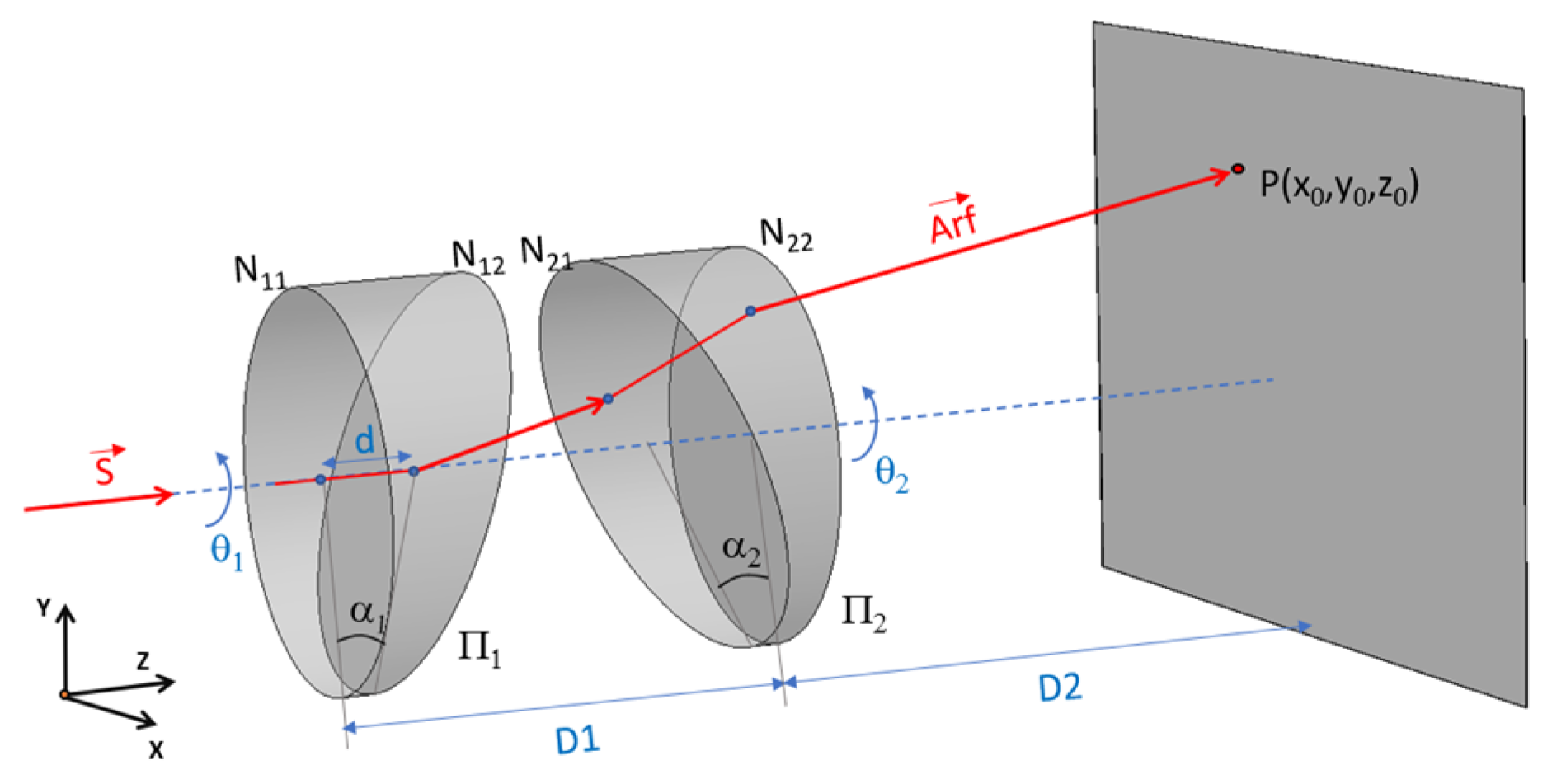
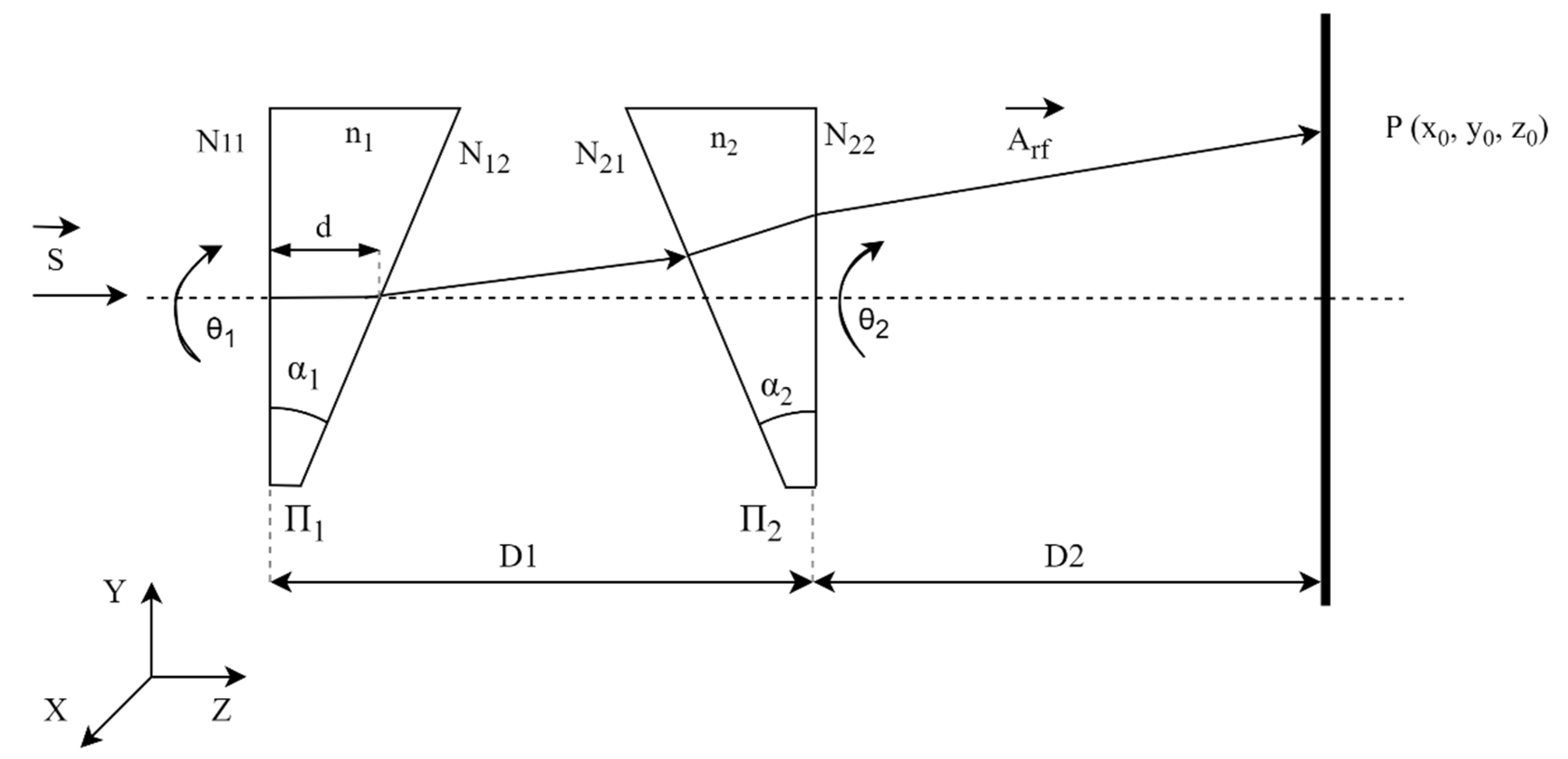
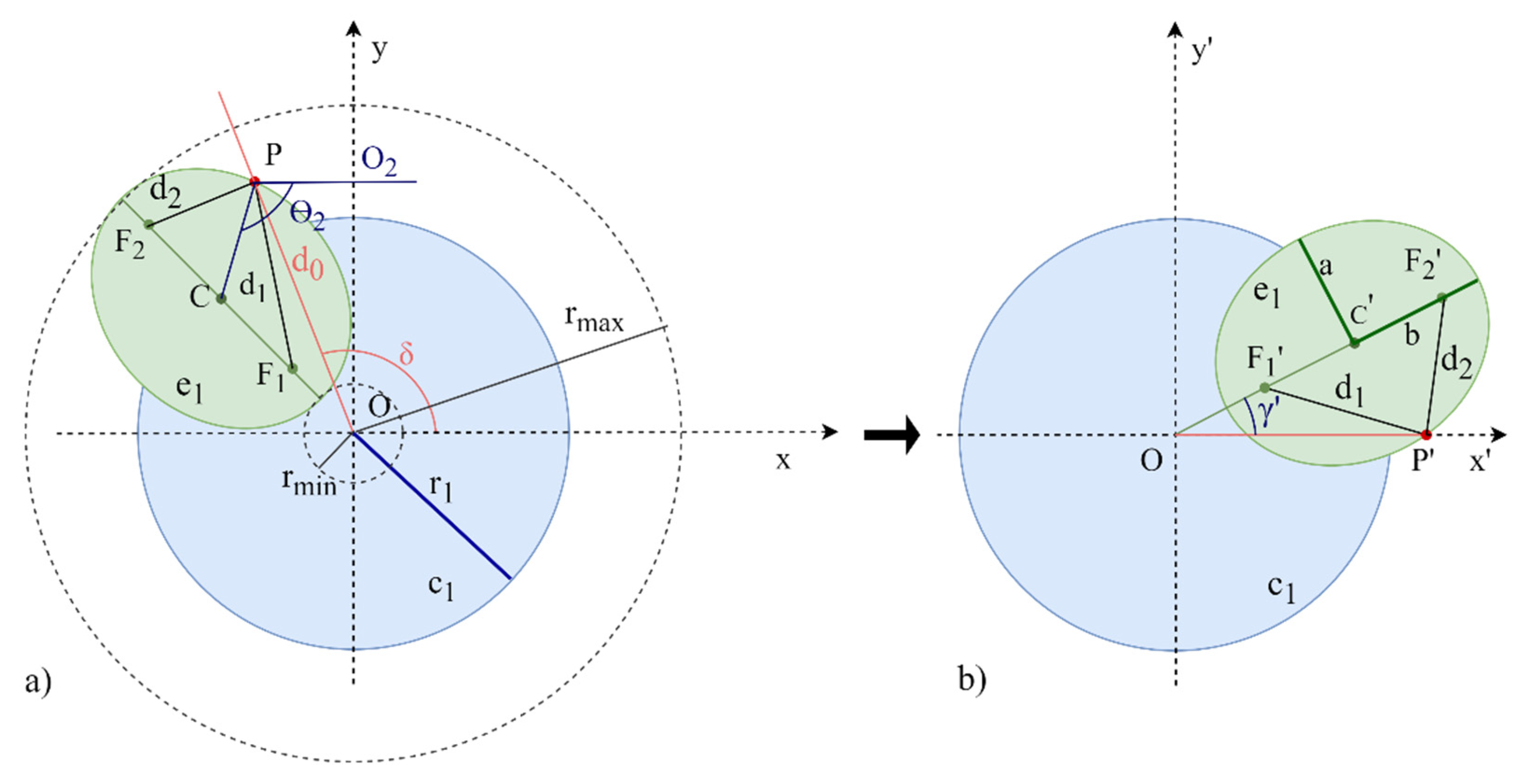
2. Proposed Inverse Solution for Risley Prisms

Given the generic Risley configuration system shown in Figure 3, the two prisms ${\pi }_1$ and ${\pi }_2$ are rotated independently about the Z axis. The surfaces of the first prism have been designated N11 and N12, and the surfaces of the second prism N21 and N22. The refractive index of the prisms is denoted n₁, and n₂ is and the wedge angle of the prisms, α₁ and α₂. The orientations of the prisms are specified by the respective rotation angles θ₁ and θ₂. The distance between the two prisms is D1, and the distance between the emergent surface of prism π₂ and the receiving screen is D2.

Assuming the prisms are identical and have the same characteristics:

$$\begin{gathered} n_1=n_2=n \\ {\alpha }_1={\alpha }_2=\alpha \end{gathered}$$

(2)

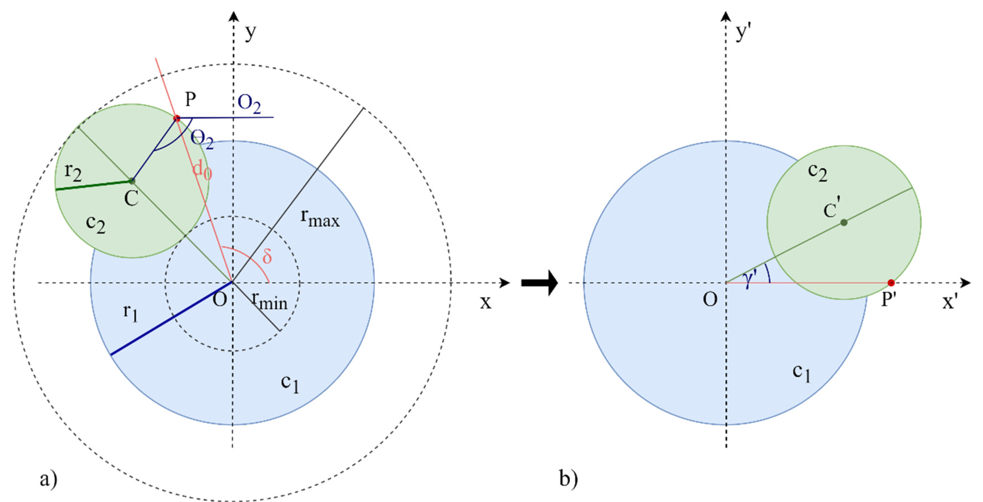
2.1. Geometric Method, Circumference Approximation

In this first approximation, Figure 4a, the geometric shape that the beam describes when the second prism ${\pi }_2$ rotates approximates a circumference $c_2$ with centre $C$at any point of the circle $c_1.$The circumference $c_1$ (with the centre at the point of origin, $O$) is described by the beam when the first prism ${\pi }_1$ rotates and there is no second prism ${\pi }_2$. Using the Forward Vector Refraction Theorem, the maximum and minimum radius that the system can reach at a given distance D2 can be calculated. The maximum radius $\left(r_{max}\right)$ is obtained when both prisms are oriented with the same angle of rotation and the minimum radius $\left(r_{min}\right)$ is obtained when the prisms are 180° out of phase. Once both values have been calculated, the primary and secondary radius ($r_1 \mathrm{and} r_2$) can be obtained.

$$\begin{gathered} r_1=r_2+r_{min} \\ {r}_2=\left(r_{max}-r_{min}\right)/2 \end{gathered}$$

(3)

Given the target point P to be reached with coordinates ($x_0, y_0$), a change of axes through the angle δ is made, Figure 4b, so that the target point P is on the X’ axis and now becomes P’ ($x_0^{\prime },y_0^{\prime }$).

Considering $y_0^{\prime }=0$ and solving the system of equations in (4) that define the radii ($r_1, r_2$), the centre point $C^{\prime }(x_c^{\prime },y_c^{\prime }$) is obtained.

$$\begin{gathered} r_1=\sqrt{x_c^{\prime }{}^2+y_c^{\prime }{}^2} \\ {r}_2=\sqrt{\left(x_c^{\prime }-x_0^{\prime }\right)2+y_c^{\prime }{}^2} \end{gathered}$$

(4)

Knowing the centre point C’, it is possible to calculate the angle ${\gamma }^{\prime }$:

$${\gamma }^{\prime }=acos\left(x_c^{\prime }/r_1\right)=acos\left(\left(r_1^2-r_2^2+x_0^{\prime }{}^2\right)/2r_1{x}_0^{\prime }\right)$$

(5)

Finally, undoing the change of coordinate axes, the rotation angle of the first prism ${\theta }_1$ is:

$${\theta }_1={\gamma }^{\prime }+\delta$$

(6)

where $\delta$ is:

$$\delta =acos\left(x_0/\sqrt{x_0^2+y_0^2} \right)$$

(7)

The centre point of the circumference $C^{\prime }(x_c^{\prime }, y_c^{\prime }$) on the X’ and Y’ coordinate axes is isolated from (5) to obtain the rotation angle of the second prism ${\theta }_2$:

$$\begin{gathered} x_c^{\prime }=r_1·cos\left({\gamma }^{\prime }\right) \\ {y}_c^{\prime }=r_1·sin\left({\gamma }^{\prime }\right) \end{gathered}$$

(8)

Translating the centre point C’ to the X and Y coordinate axes:

$$\begin{gathered} x_c=x_c^{\prime }·\cos \left(\delta \right)-y_c^{\prime }·\sin \left(\delta \right) \\ {y}_c=x_c^{\prime } ·\sin \left(\delta \right)+y_c^{\prime }·cos\left(\delta \right) \end{gathered}$$

(9)

The rotation angle of the second prism ${\theta }_2$ is the angle of the section formed by the points $\left(C, P, O_2\right)$ in Figure 4a.

$${\theta }_2=acos\left(\left(x_0-x_c\right)/\sqrt{{\left(-x_0+x_c\right)}^2+{\left(-y_0+y_c\right)}^2 }\right)$$

(10)

2.2. Geometric Method, Ellipse Approximation

The second approximation is based on an ellipse described by the beam. Using the properties of eccentricity and the focal distance of the ellipse, it is possible to obtain the rotation angles of the prisms. To obtain the rotation angles of the prisms, it is necessary to calculate the value of the semi-axis a, which depends on the wedge angle of the prisms α and the distance D2.

2.2.1. Calculation of the Semi-Axis a

The value of the semi-axis b is the value of the secondary radius r₂. On the other hand, the value of the semi-axis a must be optimised so that the error between the points calculated by the Forward Vector Refraction Theorem and by the parametric equations of the ellipse for a specific distance D2 can be minimised. The value of the semi-axis a can be optimized with different minimization methods such as those of Nelder and Mead [15,16] or Powell [17].

Once the value of the semi-axis a has been optimised for the specific distance D2, the incident angle $\epsilon$ of the laser beam on the screen can be obtained:

$$\epsilon =atan\left(a/D2\right)$$

(11)

The incident angle $\epsilon$ is constant for the optic system configuration and does not depend on the distance D2′, so it is not necessary to repeat the optimization process. It is possible to calculate a’ for any distance D2′ as:

$$a^{\prime }=D{2}^{\prime }·tan\left(\epsilon \right)$$

(12)

Once the value of the semi-axis a has been obtained, the angles of rotation of the prisms can be calculated.

2.2.2. Calculation of the Rotation Angles of the Prisms

In this approximation, the geometric shape that describes the beam, when the second prism ${\pi }_2$ rotates, approximates an ellipse $e_1$ with centre $C$ at any point of the circle $c_1.$

Since the sum of the focal distances of any point P on an ellipse is constant and equal to the length of the major axis of the ellipse (b):

$$PF1+PF2=2b\to d_1+d_2=2b$$

(13)

For simplicity, a rotation of the coordinate axes through the angle δ is made, Figure 5, so that the target point P is on the X’ axis, being now the point P’ ($x_0^{\prime },y_0^{\prime }$).

Knowing the target point P’ and the points of the focal distance F1′ ($x_1^{\prime }$,$y_1^{\prime }$) and F2′ ($x_2^{\prime },y_2^{\prime }$), the distance between them is calculated as:

$$\begin{gathered} d_1=\sqrt{\left(x_1^{\prime }-x_0^{\prime }\right)2+{\left(y_1^{\prime }-y_0^{\prime }\right)}^2} \\ {d}_2=\sqrt{{\left(x_2^{\prime }-x_0^{\prime }\right)}^2+{\left(y_2^{\prime }-y_0^{\prime }\right)}^2} \end{gathered}$$

(14)

where:

$$\begin{gathered} x_1^{\prime }=r_F^1·cos\left({\gamma }^{\prime }\right) \\ {y}_1^{\prime }=r_F^1·sin\left({\gamma }^{\prime }\right) \\ {x}_2^{\prime }=r_{F2}·cos\left({\gamma }^{\prime }\right) \\ {y}_2^{\prime }=r_{F2}·sin\left({\gamma }^{\prime }\right) \end{gathered}$$

The radius $r_{F1}$and $r_{F2}$ are the radii of the circles formed with the centre at the origin and passing through focus points F1 and F2, respectively. The focus points F1 and F2 are at the same distance from the primary radius. This distance is $\sqrt{b^2-a^2}.$

Considering $y_0^{\prime }=0$ and on the basis of Equations (13) and (14), it is possible to obtain the solution of the angle ${\gamma }^{\prime }$ between the X’-axis and the line that passes through the centre point C’ of the ellipse:

$${\gamma }^{\prime }=-acos\left(-\left(c_4-4b·c_7+c_5\right)/x_0^{\prime }·c_3\right)$$

(15)

where:

$$\begin{gathered} c_1=-4b^2·r_{F1}-4b^2·r_{F2} \\ {c}_2=r_{F1}{}^3-r_{F1}{}^2·r_{F2}-r_{F1}{r}_{F2}{}^2+r_{F2}{}^3 \\ {c}_3=2·{\left(r_{F1}-r_{F2}\right)}^2 \\ {c}_4=-c_1 \\ {c}_5=-c_2 \\ {c}_6=4b^2{r}_{F1}{r}_{F2}-r_{F1}{}^3{r}_{F2}+2r_{F1}{}^2{r}_{F2}{}^2-r_{F1}{r}_{F2}{}^3 \\ {c}_7=\sqrt{c_6+r_{F1}{}^2·{x_0^{\prime }}^2-2r_{F1}·r_{F2}·{x_0^{\prime }}^2+r_{F2}{}^2·{x_0^{\prime }}^2} \end{gathered}$$

Finally, the rotation angle of the first prism ${\theta }_1$ and the second prism ${\theta }_2$ can be determined following the same process as the circumference approximation (undoing the change of coordinate axes) through Equations (6)–(10).

2.3. Iterative Process with Geometric Method

To improve the accuracy of reaching the target point, Li et al. developed an iterative method [7] consisting of a combination of the two-step method [9] and the Forward Vector Refraction Theorem. In this paper, the two-step method is replaced with the geometric method.

In the first iteration, the exiting point of the system is assumed to be the centre $N \left(0, 0, D1\right)$ of the second surface of the prism ${\mathsf{\Pi }}_2.$ Given a target point $P \left(x_p, y_p,z_p\right)$, it is possible to calculate the rotation angles (${\theta }_1, {\theta }_2$) of the prisms by the geometric method. Then, by substituting the rotation angles into the Forward Vector Refraction Theorem, the corresponding exit point $N=\left(x_n,y_n,z_n\right)$ and the tracking point $P_r=\left(x_{rp},y_{rp},z_{rp}\right)$ is obtained. The tracking point $P_r$ has a deviation (${\phi }_x, {\phi }_y$) from the target point P, with ${\phi }_x=x_p-x_{rp}$ and ${\phi }_y=y_p-y_{rp}$.

In the second iteration, taking the point $P_i=\left(x_i, y_i,z_i\right)=\left(x_p+{\phi }_x, y_p+{\phi }_y, D2\right)$ as the target point of the system, it is possible to calculate the rotation angles (${\theta }_1, {\theta }_2$) of the prisms by the geometric method. This process is iterated until the separation distance between the tracking point P_r and the target point $P$ meets the given accuracy requirement $\delta .$

The steps to implement the geometric method in an iterative process are:

Step 1. Given a target point $P \left(x_p, y_p,z_p\right),$ assume that the initial point is $N \left(x_n,y_n,z_n\right)=\left(0, 0, D1\right)$ on prism ${\mathsf{\Pi }}_2$ and that the deviation (${\phi }_x, {\phi }_y$) is zero.

Step 2. Calculate the rotation angles (${\theta }_1, {\theta }_2$) of the two prisms using the geometric method by considering the initial point $P_i=\left(x_i, y_i,z_i\right)=\left(x_p+{\phi }_x, y_p+{\phi }_y, D2\right)$ as the point to be reached.

Step 3. Update the current exit point $N=\left(x_n,y_n,z_n\right)$ and the current target point $P_r=\left(x_{rp},y_{rp},z_{rp}\right)$ substituting the rotation angles into the Forward Vector Refraction Theorem.

Step 4. Calculate the error Δ between the tracking point and the current target point on the receiving screen as: $\Delta =\sqrt{{\left(x_{rp}-x_p\right)}^2+{\left(y_{rp}-y_p\right)}^2+{\left(z_{rp}-z_p\right)}^2}$. If the error is less than the error threshold ($\Delta <\delta$) the rotation angles (${\theta }_1, {\theta }_2$) are considered to be determined. If not, update the deviation ${\phi }_x=x_i-x_{rp}, {\phi }_y=y_i-y_{rp}$ and go to step 2.

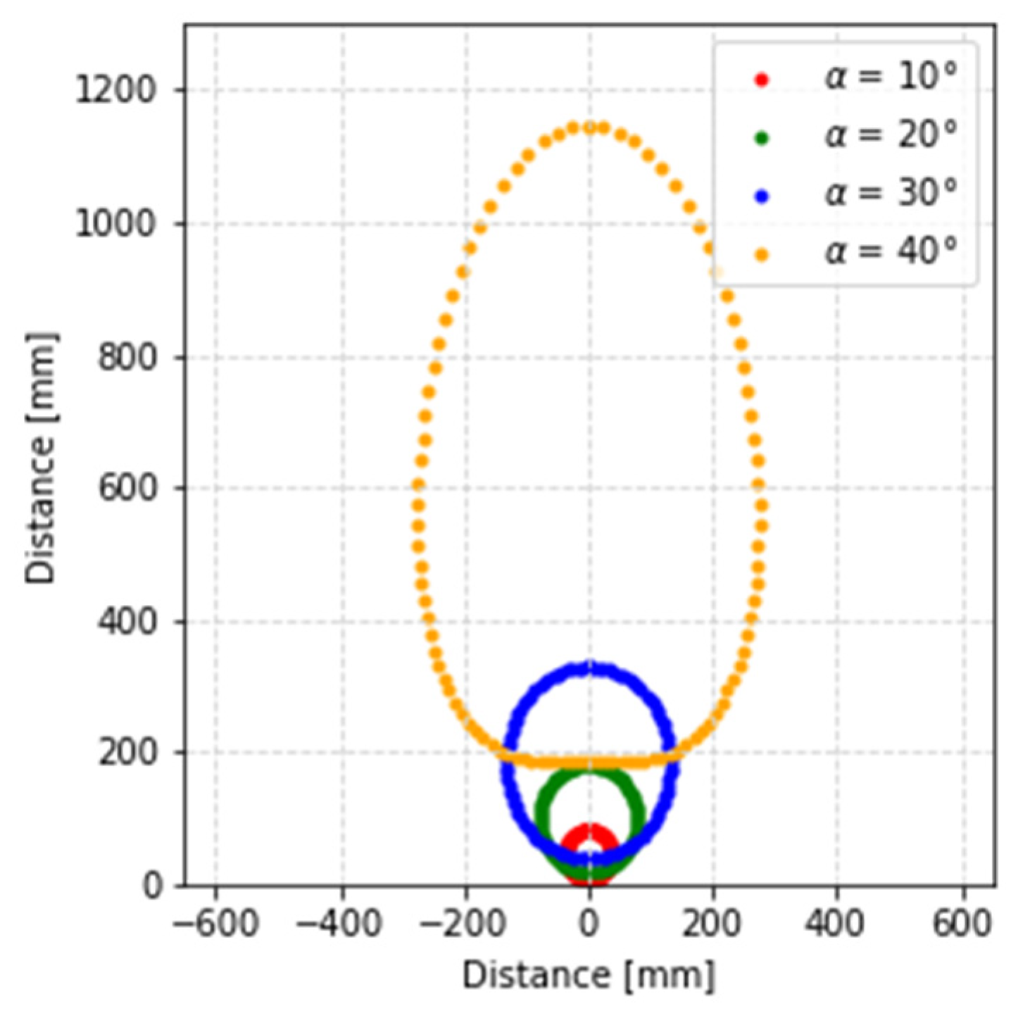
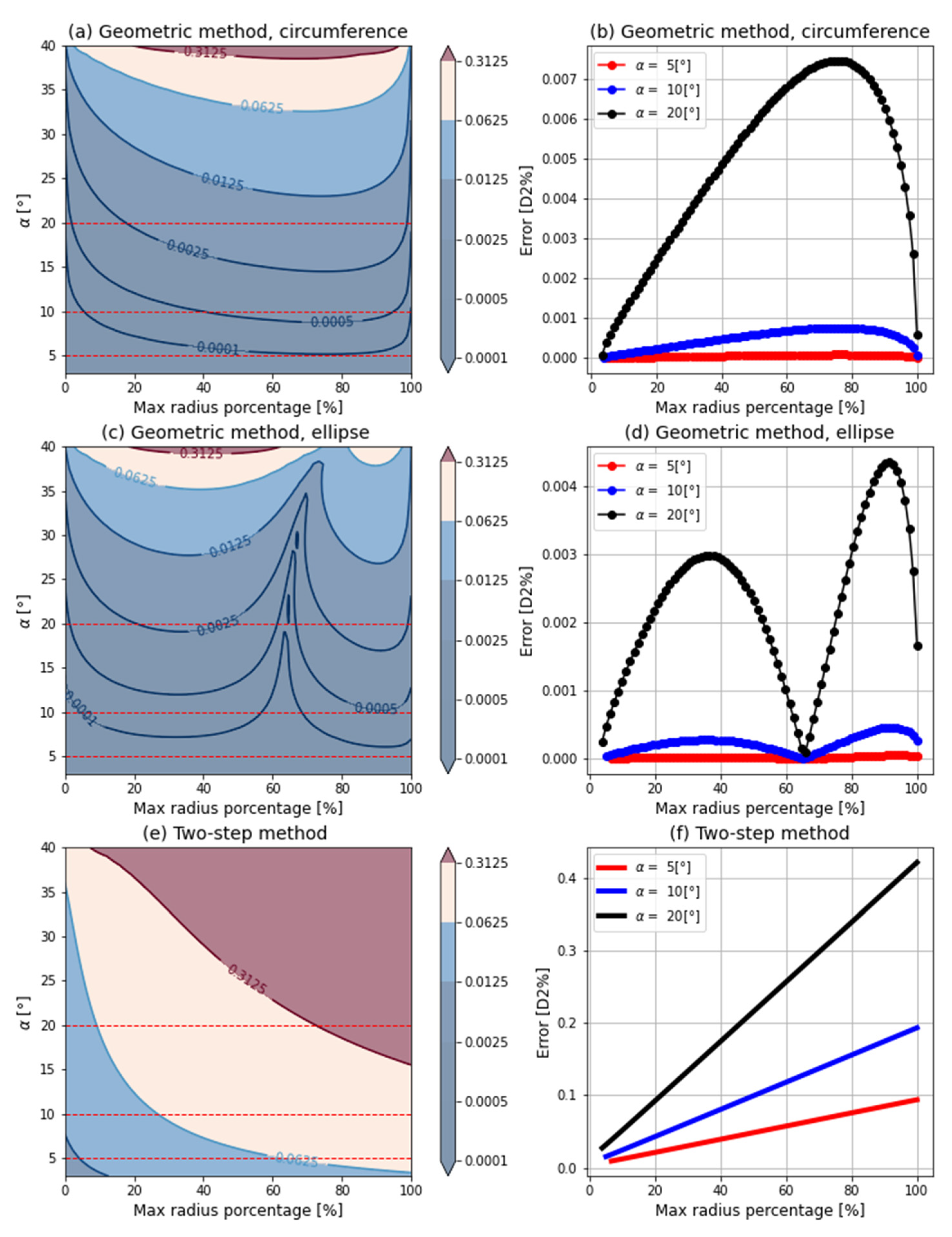
3. Results of the Geometric Method

In order to evaluate how good a method is, it is necessary to evaluate its accuracy and efficiency. The first part of the results section presents an analysis of these two aspects of the one-step method (geometric method: ellipse and circumference approximation) and compares the results with the two-step method [9]. The second part presents an analysis of the iterative process and compares the results with the method of Li et al. [7].

The parameters of two identical prisms used to obtain the results were the refractive index (n = 1.517), the diameter of the prisms (25.4 mm), the distance between the two prisms (D1 = 40 mm), and the thickness of the thinnest end ($d_0$ = 2.75 mm).

Three parameters were modified to analyse the behaviour of the approximations under different conditions. The distance between the emergent surface of the prism ${\pi }_2$ and the receiving screen D2 was given values of between 500 mm and 16.384 km, the wedge angle α was changed between 2° and 40°, and the error threshold δ for the iterative process was given values of between $0.1 \mathsf{\mu }\mathrm{m}$and $1 \mathrm{pm}$.

The computer used to obtain the following results has an AMD Ryzen 5 CPU and 8 GB memory, and the code was developed in C++.

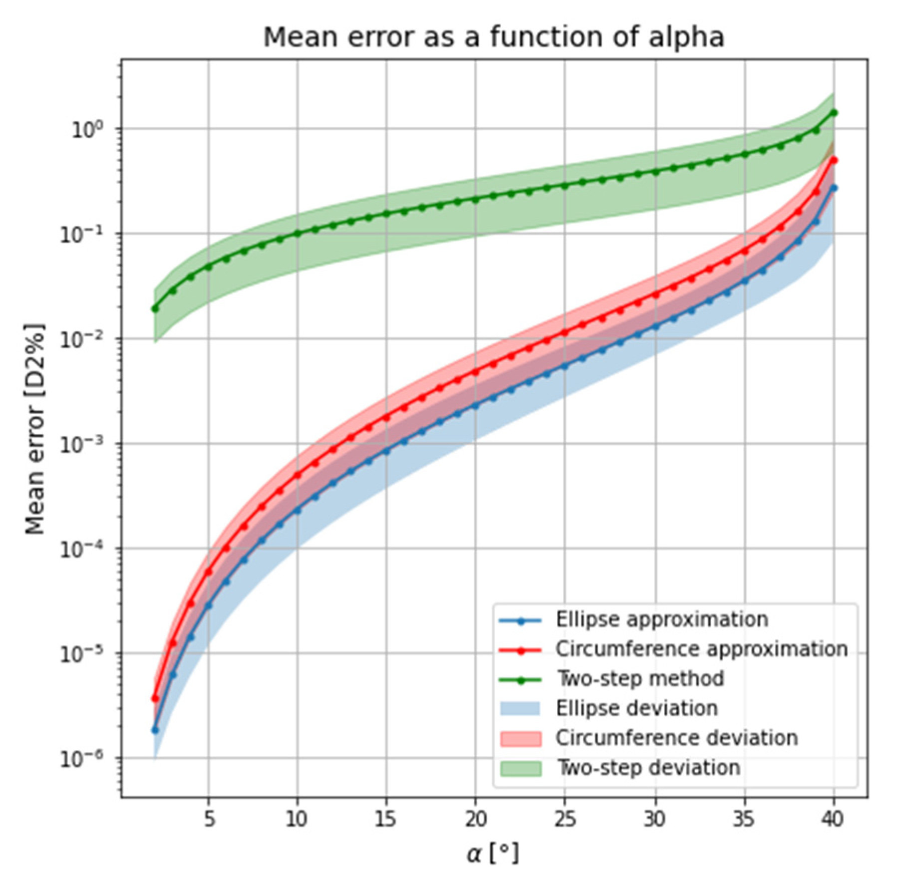
3.1. Comparison of the Errors Obtained with the Geometric Method and the Two-Step Method

The accuracy in the direction of the laser beam to any point in space varies radially and also depends on the wedge angle α. To analyze the accuracy of the method, the error is calculated, where the error is the difference between the target point and the point that has been reached with the method used. The two-step method [9] developed by Yajun Li is used as a reference in this paper to show the improvement provided by the geometric method.

For the three methods (geometric method-circumference, geometric method-ellipse and the two-step method), as can be seen in Figure 6a,c,e, the error increases with the wedge angle. Three wedge angle values were also selected to observe their profile as a function of the radius, Figure 6b,d,f. The two-step method [9] (Figure 6e,f) has radial behavior, with the error increasing with the radius. However, in the geometric method (Figure 6a–d), the minimum error is obtained at the minimum and maximum radius. This is because the laser beam does not actually describe a circumference but is closer to an ellipse, and the radius of the circumference is the same as the semi-axis b of the ellipse. Moreover, in the ellipse approximation (Figure 6c,d), the error is minimized such that when the radius is 65% of the maximum radius, a minimum error occurs.

In all three methods, the error depends on the wedge angle of the prisms α. However, the error as a percentage of the distance D2 does not change even if the distance increases. Considering a target distance (D2) of 1 m, Figure 7 shows the mean error as a percentage of the distance D2 and the shadow regions correspond to the standard deviation of the mean error obtained for each wedge angle of the prisms. The mean error was obtained from a set of eighty points. This set of points was in turn obtained on a straight line for an azimuth angle of 45°. As the error is radial, it does not matter which angle is considered.

It can be seen from Figure 7 that the error obtained by the ellipse approximation is smaller than the error obtained by the circumference approximation. The error of the circumference approximation is approximately twice that of the ellipse approximation. However, both approximations of the geometric method have a smaller error than the two-step method.

Another important aspect to consider is the calculation time required to obtain the desired data, the results of which are shown in

Table 1. Mean time and deviation of the geometric method and the two-step method obtained from a total set of 78,400 points.

	Geometric Method		Two-Step Method
	Circumference Approximation	Ellipse Approximation
$\mathrm{Mean} \mathrm{time} \left(\mathsf{\mu }\mathrm{s}\right)$	2.7257	4.3378	9.6737
$\mathrm{Deviation} (\mathsf{\mu }\mathrm{s})$	0.4754	0.5015	7.3917

. For this, we used a set of 4900 points, which contains points for seventy different angles of the whole possible region and seventy different radii between the minimum and maximum values. This set of points was repeated sixteen times, giving a total of 78,400 points to calculate the mean time and the deviation.

The ellipse approximation had a longer mean computation time than the circumference approximation. The circumference approximation was about 1.6 times faster than the ellipse approximation. However, both approximations of the geometric method were faster than the two-step method.

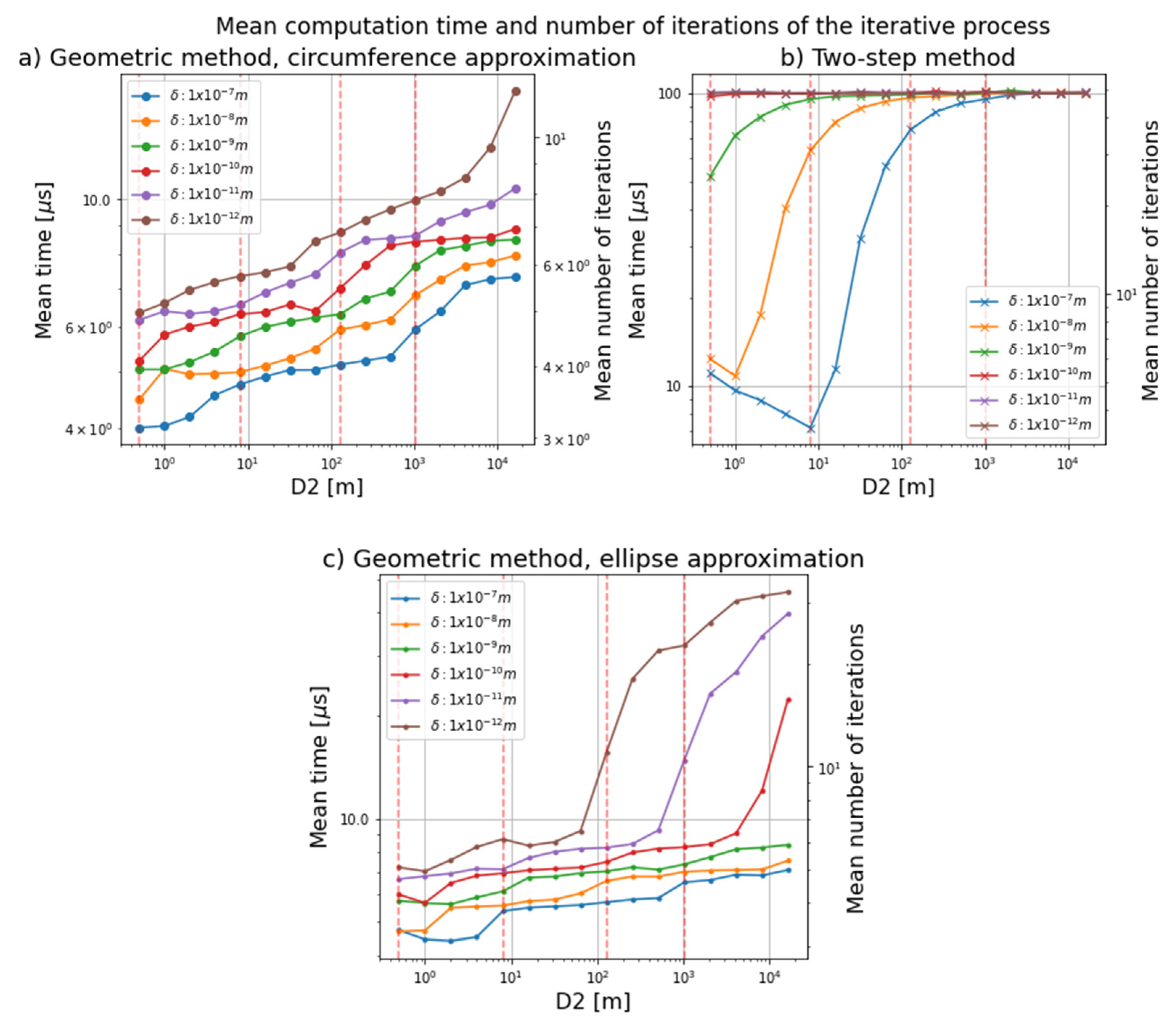
3.2. Comparative Results of the Error with the Iterative Process

The geometric method was implemented in an iterative process to increase the accuracy and then compared with the method developed by Li et al. [7], which also follows an iterative process.

The results shown below were obtained for a wedge angle α of 10°. The mean computation time and the number of iterations that each method took to reach the required error threshold were calculated, with the results shown in Figure 8. Each point represented in the graphs in Figure 8 is the mean time obtained for a set of 40,000 points scattered all over the region that the Risley system can reach. The left y-axis shows the mean time taken by each method, and the right y-axis shows the number of iterations taken. The graphs in Figure 8a,c show the results obtained for the iterative process with, respectively, the circumference and ellipse approximations of the geometric method. The graph in Figure 8b shows the results obtained with the iterative method proposed by Li et al. [7]. The dashed red lines are the D2 values taken as reference to show the mean number of iterations in

Table 2. Mean number of iterations of each method for different distances D2 and a specific error threshold.

D2 (m)	Δ (m)	Geometric Method		Two-Step Method
		Circumference Approximation	Ellipse Approximation
0.5	$1·{10}^{-7}$	3.00	3.21	5.12
8		3.76	3.78	3.30
128		4.06	4.04	38.10
1024		4.72	4.64	48.56

.

Figure 8 shows how the iterative process has a shorter computation time when using the geometric method proposed in this paper than the method developed by Li et al. [7] for any distance D2 and error threshold. The shortest time taken by the iterative process with the geometric method to obtain the final rotation angles is 4 μs, whereas the corresponding value for the two-step method is 7 μs. This time is equivalent to three iterations performed using the iterative process with the geometric method and about four iterations with the two-step method.

The maximum number of iterations that the iterative process can reach is 50, a value that was established after several tests found that if the method is unable to reach the required threshold error in 50 iterations, it will never do so.

The graph in Figure 8b shows that with Li et al. method [7] for large distances (more than 100 m) and for very small error thresholds $\left(1 \mathrm{nm}\right)$ the results are obtained on average in $100 \mathsf{\mu }\mathrm{s}$. This is because the method has reached the maximum number of iterations (i.e., the two-step method does not achieve error thresholds smaller than $1 \mathrm{nm})$. In contrast, an error threshold of up to $1 \mathrm{pm}$ can be achieved for any distance D2 up to 16.384 km with the circumference approximation (Figure 8a), while a margin of error of $1 \mathrm{nm}$ is reached for any distance D2 with the ellipse approximation (Figure 8c).

Table 2 shows the average number of iterations each method needed to reach a margin of error of $1·{10}^{-7} \mathrm{m}$, the least accurate margin of error, and for different distances D2. It is observed that the results for the iterative process with the ellipse and circumference approximations are quite similar in the case where the margin of error is not so restrictive. However, it can also be seen that the two-step method presents good accuracy only for small distances and that the number of iterations increases with increasing distance.

From the analysis of the mean time and mean number of iterations required by the three methods, it can be concluded that the method with the best results for the iterative process is the geometric method with circumference approximation. This method achieves a higher accuracy for smaller and larger distances and reaches accuracies three orders of magnitude lower than the other methods.

4. Conclusions

Many studies have been carried out on the inverse problem and different solutions have been proposed, including the third-order theory [8], the inverse solution [4], the two-step method [9,10,11], and the iterative method [7]. In this paper, a geometric method is proposed to solve the rotation angles for a given target trajectory in less computing time and with high accuracy.

Two approximations were made for the geometric method, and the accuracy and time obtained by both were analyzed. The error of the circumference approximation is approximately twice that of the ellipse approximation. However, the ellipse approximation has a longer computation time than the circumference approximation.

The geometric method was also compared with the two-step method [9], with the results showing that the geometric method is faster and more accurate.

Until now, the most accurate method was the iterative method [7]. Therefore, the geometric method was implemented in an iterative process to determine whether it reduces computation time and improves accuracy. It was found that Li et al. iterative method [7] obtains good time and accuracy results for small D2 distances, while the iterative process with the geometric method obtains good results for both small and large D2 distances. In addition, the iterative method [7] takes more iterations to reach the established error threshold, and, therefore, the computation time is longer than the iterative process with the geometric method. The method developed in this work achieves an accuracy of $1 \mathrm{pm}$ in only three iterations.

That is, the geometric method offers a far better accuracy solution for the inverse problem of Risley systems to prevent laser beam misalignment. Solving the inverse problem enables applications that involve the control of dual-prism rotary motions, including multimode beam tracking in the field of airborne laser communications, the monitoring of containers in harbor operations, and target tracking in the military domain. Moreover, the geometric method could be used in applications that require high degrees of accuracy, such as lithography, stereolithography, or 3D printing.

Future research will use the geometric method in various real applications.

References

1. Jianfeng, S.; Liren, L.; Maojin, Y.; Lingyu, W.; Mingli, Z. The effect of the rotating double-prism wide-angle laser beam scanner on the beam shape. Optik 2005, 116, 553–556. [Google Scholar] [CrossRef]
2. Church, P.; Matheson, J.; Cao, X.; Roy, G. Evaluation of a steerable 3D laser scanner using a double Risley prism pair. Degrad. Environ. Sens. Process. Disp. 2017, 10197, 101970O. [Google Scholar] [CrossRef]
3. Li, A.; Liu, X.; Sun, J.; Lu, Z. Risley-prism-based multi-beam scanning LiDAR for high-resolution three-dimensional imaging. Opt. Lasers Eng. 2022, 150, 106836. [Google Scholar] [CrossRef]
4. Amirault, C.T.; DiMarzio, C.A. Precision pointing using a dual-wedge scanner. Appl. Opt. 1985, 24, 1302–1308. [Google Scholar] [CrossRef] [PubMed] [Green Version]
5. Souvestre, F.; Hafez, M.; Régnier, S. DMD-based multi-target laser tracking for motion capturing. Emerg. Digit. Micromirror Device Based Syst. Appl. II 2010, 7596, 75960B. [Google Scholar] [CrossRef]
6. Yang, Y. Analytic Solution of Free Space Optical Beam Steering Using Risley Prisms. J. Light. Technol. 2008, 26, 3576–3583. [Google Scholar] [CrossRef]
7. Li, A.; Gao, X.; Sun, W.; Yi, W.; Bian, Y.; Liu, H.; Liu, L. Inverse solutions for a Risley prism scanner with iterative refinement by a forward solution. Appl. Opt. 2015, 54, 9981–9989. [Google Scholar] [CrossRef] [PubMed]
8. Li, Y. Third-order theory of the Risley-prism-based beam steering system. Appl. Opt. 2011, 50, 679–686. [Google Scholar] [CrossRef] [PubMed]
9. Li, Y. Closed form analytical inverse solutions for Risley-prism-based beam steering systems in different configurations. Appl. Opt. 2011, 50, 4302–4309. [Google Scholar] [CrossRef] [PubMed]
10. Lu, Y.; Zhou, Y.; Hei, M.; Fan, D. Theoretical and experimental determination of steering mechanism for Risley prism systems. Appl. Opt. 2013, 52, 1389–1398. [Google Scholar] [CrossRef] [PubMed]
11. Zhou, Y.; Lu, Y.; Hei, M.; Liu, G.; Fan, D. Motion control of the wedge prisms in Risley-prism-based beam steering system for precise target tracking. Appl. Opt. 2013, 52, 2849–2857. [Google Scholar] [CrossRef] [PubMed]
12. Li, A.; Sun, W.; Gao, X. Nonlinear inverse solution by the look-up table method for Risley-prism-based scanner. Opt. Appl. 2016, XLVI, 4. [Google Scholar] [CrossRef]
13. Alajlouni, S. Solution to the Control Problem of Laser Path Tracking Using Risley Prisms. IEEE/ASME Trans. Mechatron. 2016, 21, 1892–1899. [Google Scholar] [CrossRef]
14. Bravo-Medina, B.; Strojnik, M.; Garcia-Torales, G.; Torres-Ortega, H.; Estrada-Marmolejo, R.; Beltrán-González, A.; Flores, J.L. Error compensation in a pointing system based on Risley prisms. Appl. Opt. 2017, 56, 2209–2216. [Google Scholar] [CrossRef]
15. Nelder, J.A.; Mead, R. A Simplex Method for Function Minimization. Comput. J. 1965, 7, 308. [Google Scholar] [CrossRef]
16. Singer, S.; Singer, S. Efficient Implementation of the Nelder-Mead Search Algorithm. Appl. Numer. Anal. Comput. Math. 2004, 1, 524–534. [Google Scholar] [CrossRef]
17. Powell, M. On trust region methods for unconstrained minimization without derivatives. Math. Program. 2003, 97, 605–623. [Google Scholar] [CrossRef]
Figure 1. Risley system diagram in 3D.
Applsci 12 11087 g001
Figure 2. Representation of the different geometric shapes that the beam describes depending on the wedge angle of the prisms.
Applsci 12 11087 g002
Figure 3. Risley system diagram.
Applsci 12 11087 g003
Figure 4. Rotation of the coordinate axes of circumference approximation. (a) represents the original axes (X, Y); (b) represents the rotated axes (X’, Y’) though the angle δ.
Applsci 12 11087 g004
Figure 5. Rotation of the coordinate axes of the ellipse approximation. (a) represents the original axes (X, Y); (b) represents the rotated axes (X’, Y’) though the angle δ.
Applsci 12 11087 g005
Figure 6. Error of the two approximations for different values of wedge angle α and radius of the target point. (a) represents a heat map with the error obtained by the circumference approximation; (b) represents the error profile obtained by the circumference approximation; (c) represents a heat map with the error obtained by the ellipse approximation; (d) represents the error profile obtained by the ellipse approximation; (e) represents a heat map with the error obtained by the two-step method [9]; (f) represents the error profile obtained by the two-step method [9].
Applsci 12 11087 g006
Figure 7. Mean error as percentage of D2 for each value of the prism angle α.
Applsci 12 11087 g007
Figure 8. Mean computation time as a function of distance D2 for each error threshold. (a) represents the mean computation time obtained using the iterative process with the geometric method (circumference approximation) for each error threshold; (b) represents the mean computation time obtained using the iterative method with the two-step method for each error threshold; (c) represents the mean computation time obtained using the iterative process with the geometric method (ellipse approximation) for each error threshold.
Applsci 12 11087 g008