Robust Evaluation of Reference Tilt in Digital Holography

Abstract

A robust approach is designed to evaluate the reference tilt angle (RTA) accurately and efficiently by local Gaussian fitting (LGF) for the distribution of one frequency peak on a spatial spectrum plane (SSP). The novel method proposed can avoid enlarging the data array on either a hologram or an SSP and then alleviate the computing burden on information processing hardware. Moreover, the RTA precision can be improved by one order of the magnitude in certain ranges, which benefits not only the accurate image recovery in an off-axis digital holography (DH) display but also the thorough removal of the tilt error effect on the image quality in phase-shifting digital holography (PSDH). The error source of the frequency peak position is analyzed theoretically and the principle with detailed steps is described. Several cases of numerical simulations have been carried out to demonstrate the availability and accuracy of this robust RTA evaluation method.

1. Introduction

Spectrum analysis in the Fourier domain [1,2,3] provides an alternative way to extract some important optical information, which is not available in the space domain. The Fourier domain spectrum then plays an important role either in improving the resolution in super-resolution imaging [4,5,6] or in solving the parameters necessary for object wave recovery in digital holography (DH) [7,8,9,10,11,12]. Because the imaging resolution of an optical system is constrained by the cut-off frequency of the imaging system, researchers provide several kinds of methods to break through the resolution limitation. Optical devices are inserted in the experiment setup to collect the high-frequency spectrum in digital holography so that the imaging resolution can be improved. For example, Liu C. et al. [13] introduced a grating between the test sample and the charge coupled device (CCD), and then the corresponding high-frequency component can be projected onto the small CCD chip. This method is, in fact, a kind of multiplexing technique since the high-frequency spectrum is reused in the holography imaging system. The imaging resolution improves with receiving these collected high-frequency spectra. However, using gratings to ensure the acceptance of more spectra increases the cost and operation complexity of the experiment. Structured illuminating light [4] is also used to break through the resolution bottleneck of the coherent imaging system. Nine exposures are necessary to gain more high-frequency spectra across three imaging directions. This multi-frame recording method consumes more time and only suits static imaging with super-resolution in biomedical research. A spatial-temporal light sheet [14,15] is then used in biomedical imaging microscopy to improve image quality.

In both off-axis DH (OADH) and in-line PSDH [16,17,18,19] applications, the Fourier domain spectrum is also beneficial to separate the needed information for multiplexing techniques [20,21], especially for the detection of RTA.

RTA detection is significant to eliminate the negative effect of the reference tilt on the imaging quality in in-line PSDH [22] and to remove the carrier wave in the object waves reconstructed in OADH [23]. Recently, tilt reference has been suggested in OADH and PSDH where reference tilt information is recorded on a hologram [24] or extra fringes [25,26]. In all these methods, spectrum detection and operation are inevitably needed. During the process of the corresponding spectrum detection, the precision is limited by the size of the frequency pixels (FPs) on the SSP, which is always determined by the parameters of the recording device CCD. The CCD performance has been impeded by the slow development of modern workmanship. The discrete pixel of the recording device leads to corresponding discrete spectrum distribution in the Fourier frequency domain, and naturally, the precision of the spectrum location is limited by the size of FP on the SSP. Many researchers have attempted to improve the accuracy of the spectrum locating by decreasing the pixel size in the Fourier domain so that the data array on the SSP is enlarged in the Fourier domain [27,28,29]. Whereas most of these spectrum location-finding methods reported impose heavy loads on the computers, the efficiency is low in improving the precision.

Here a robust method is provided to detect the RTA in DH with high precision, efficiency, and stability. By introducing local Gaussian fitting (LGF) [30], the specific equation of the spectrum distribution is established in the computer, and then the frequency peak location is fixed by it for RTA calculation. There are many merits for this frequency spectrum fitting method. Firstly, this method has the capability to detect the RTA value accurately because the fitted function predicts the analytic solution of the spectrum distribution by theory analysis and analytical simulation. Secondly, the proposed method is efficient compared with the conventional extrapolating method [27], zero-padding [28], and least-squares iteration method [29] since only a few pixels around the targeted pixel on the SSP are used. The third merit of the method is that it releases the requirement on the hardware of the information processing system. The principle of this method is described first; then, the simulations are conducted to investigate its performance, with the conclusions following last.

2. Principles

The hologram recording setup for both OADH and PSDH have been reported [24,26], respectively. Supposing the reference tilt is determined by the two angles θ_x and θ_y across x and y directions, respectively, the reference wave can be written as

$$\mathit{R}\left(x,y\right)=A_r\exp \left[-i\frac{2\pi }{\lambda }(x\sin {\theta }_x+y\sin {\theta }_y)\right]$$

(1)

where A_r and λ are the real amplitude and the wavelength of the reference wave, respectively, and i is the imaginary unit. Commonly the real amplitude A_r is always chosen as a constant in DH. In Equation (1), θ_x and θ_y represent RTA and bring about the periodic stripes on the fringes after its interference with the zero frequency part of the objective wave. For the object wave, there must exist a sufficient zero frequency component so that the corresponding spectrum can be detected in the Fourier transform domain. The transparent sample with low diffraction can satisfy this requirement naturally. However, for the object with strong diffraction, the energy of the zero frequency spectrum is not so powerful to find the carrier frequency after the Fourier transform. So a plane wave on-axis is always necessary to supply the zero frequency ingredient in the object wave [24] or an additional frame of a two-plane wave interference is captured for RTA detection [25,26] under the condition of strong diffraction. To make the zero frequency component of the Fourier transform clear, the object wave is expressed separately as

$$\mathit{O}\left(x,y\right)={\mathit{O}}_1\left(x,y\right)+{\mathit{O}}_2\left(x,y\right)$$

(2)

where O₁(x, y) is the zero frequency component in the objective wave and can be seen as an on-axis plane wave with constant amplitude A₁ and phase φ₁

$${\mathit{O}}_1=A_1\exp \left[-i{\phi }_1\right]$$

(3)

The other part of Equation (2) O₂(x, y) is the non-zero frequency wave with object information in the complex amplitude

$${\mathit{O}}_2\left(x,y\right)=A_2\left(x,y\right)\exp \left[-i{\phi }_2\left(x,y\right)\right]$$

(4)

The supposing three waves interfere on the recording plane and the hologram is

$$I\left(x,y\right)=\left[R\left(x,y\right)+{\mathit{O}}_1+{\mathit{O}}_2\left(x,y\right)\right]{\left[R\left(x,y\right)+{\mathit{O}}_1+{\mathit{O}}_2\left(x,y\right)\right]}^{\ast }$$

(5)

where ‘*’ represents the conjugation. After the Fourier transform is operated on the hologram of Equation (5), the frequency spectrum distribution can be written in [26]

$$F\left(u,v\right)=A_r{A}_1\left[\delta \left(u+u_0,v+v_0\right)\exp (i{\phi }_1)+\delta \left(-u+u_0,-v+v_0\right)\exp (-i{\phi }_1)\right]+F_h\left(u,v\right)$$

(6)

where u and v are frequency-pixelated coordinates on SSP. Obviously, the first term in Equation (6) is the spectrum with distributions like two delta functions from the interference of two plane waves with the tilt angles θ_x and θ_y. The second term F_h (x, y) on the right side of Equation (6), includes the other spectra from the Fourier transform of Equation (5). Most of the intensity distribution of F_h (x, y) is weak compared with the first terms of Equation (6), so the center of the spectra can be detected by searching the strongest point on the SSP in the Fourier frequency domain. The coordinates u₀ = sin θ_x/λ, v₀ = sin θ_y/λ are the centers of the two delta functions in Equation (6) [24]. It should be two ideal spots with the maximum value at their centers on SSP in theory. Because of the disturbance of the other part in Equation (6), the spots always become irregular. Since fast Fourier transforms are commonly carried out digitally in a computer, u and v are not continuous and Equation (6) is a discrete function. Naturally, u₀ and v₀ are not an exact point on SSP either. The minimum unit for u, u₀ and v, v₀ are denoted as Δu and Δv, respectively

$$\Delta u=\frac{1}{M\Delta x},\Delta v=\frac{1}{N\Delta y}$$

(7)

where M, N are the pixel numbers along the horizontal and vertical directions in the recording plane with the pith of Δx and Δy. So the precision here is affected by both the CCD pixel size and the CCD matrix size. In the computer, the variants u and v or parameters u₀ and v₀ are expressed as

$$u=m\Delta u,v=n\Delta v,u_0=m_0\Delta u,v_0=n_0\Delta v$$

(8)

where m, n, m₀, n₀ are all integral numbers in order on the SSP to represent the location of the spectrum. After the spectrum with the maximum value detected, the numbers m₀ and n₀ are determined. Then using Equations (7) and (8), the RTA can be calculated by

$${\theta }_x=si{n}^{-1}[\lambda m_0/(M\Delta x)],{\theta }_y=si{n}^{-1}[\lambda n_0/(N\Delta y)]$$

(9)

The precision of the calculated RTAs are decided by the sizes of the frequency units (FPs) Δu and Δv on SSP. Smaller Δu and Δv predict higher precision of RTA.

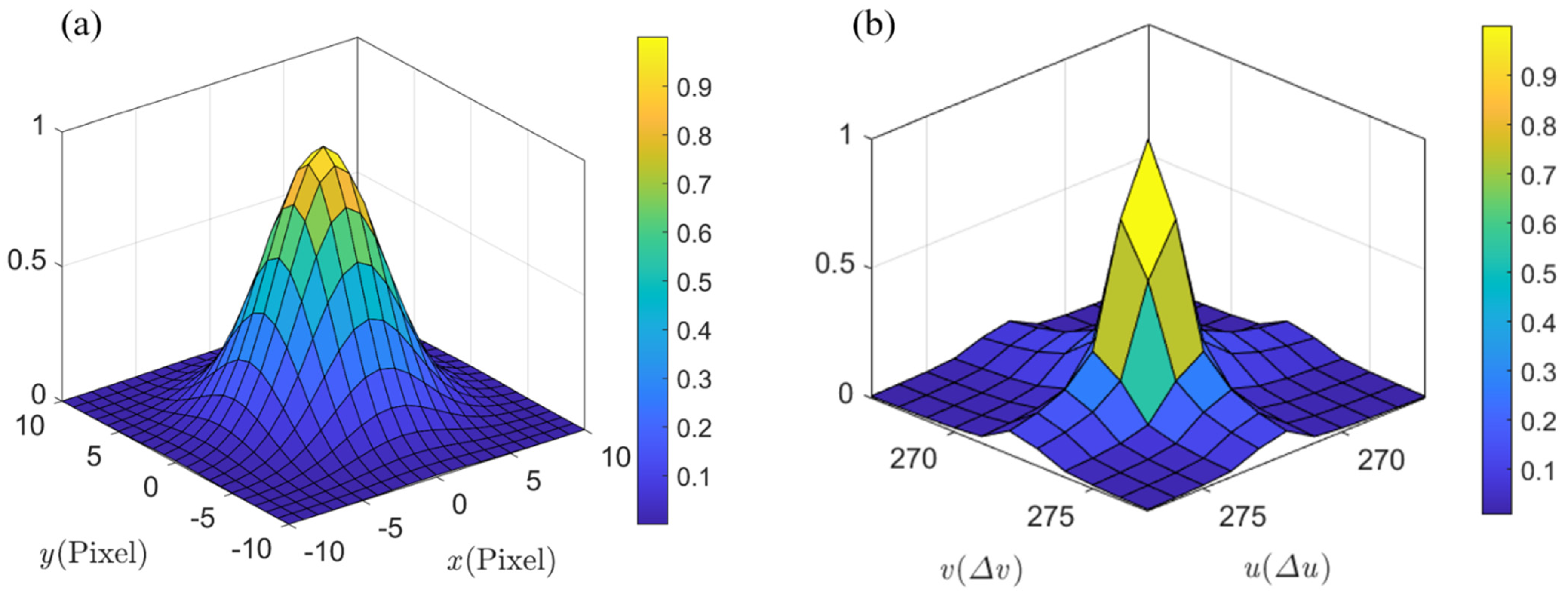
Figure 1a shows the symmetric distribution of one Gaussian function normalized by the maximum value at its center in the spatial domain. One of the frequency peaks from the Fourier spectra of two plane waves interference fringe is depicted in Figure 1b. Since the two distributions are similar, the best choice should be a Gaussian function to fit the real distribution of a frequency peak on the SSP. For the spectra regime of the off-axis holography, the distribution should be a delta function of Equation (6) in theory prediction, which should be two narrow peaks without any width. But for a specific practice, the spectra become a round spot with a certain area because of the diffraction effect from the limited aperture of the recording system under the constraint of the CCD sensor. Naturally, the spot should be a symmetrical distribution. If the distribution is a continuous function, the center point of the spot can be detected by searching its maximum value. Unfortunately, the spectra can only be expressed as a discrete distribution since it is the result of a discrete fast Fourier transform in a digital computer. The size of the minimum unit Δu and Δv is determined by the size of the hologram and the size of the pixels on it in Equation (5). The absolute value of the spectrum shown in Figure 1b is, in fact, averaged in one block or FP (Δu, Δv). The FP with the biggest absolute value can be located easily by the corresponding count number, but it is impossible to calculate the exact locations of the center of the delta function in Equation (6) unless the points (±u₀, ±v₀) fall exactly right at the center of one FP. In the specific experiment, it is always impossible to fix the RTA values exactly to satisfy this condition. Mostly, the location of the spectrum decided by RTA mismatches with any FP center. This misplacement renders an error in the calculation result of RTA and then degrades the image quality by the residue phase error. Of course, the smaller the block size denoted by Δu and Δv, the less phase error from the mismatch. So many endeavors have been made to decrease the FP size on the SSP. These up-sampling methods, including extrapolation [27] and zero padding [28], increase the data array of the hologram or SSP and then impose heavy storage and computation loads on computers very quickly [27,28]. On the other hand, the distribution of the Fourier frequency spectrum has its own law so that a proper function target can increase the fitting efficiency and improve the accuracy of the Fourier frequency spectrum location. Gaussian functions are used to express some distributions like the point spread function and delta function [30]; here, a method is provided to calculate the more accurate value of RTA after constructing a function of one frequency peak distribution by Gaussian fitting.

After the center of the frequency peak is detected, a local area including several Δus and Δvs is chosen around point (u₀, v₀) and the values of neighboring FPs can be used to predict the local distribution of the spectra by Gaussian formula

$$F_l\left(u,v\right)=A\exp \left[-\frac{{\left(u-u_{0l}\right)}^2}{2{\sigma }_u^2}-\frac{{\left(v-v_{0l}\right)}^2}{2{\sigma }_v^2}\right]+C$$

(10)

where A and C are two constants, σ_u and σ_v are the two standard errors variants u and v. The values of σ_u and σ_v can be chosen commonly and there is no need to optimize them. In Equation (10), u_0l and v_0l are the two coordinates of the peak tip, which can be calculated by

$$\frac{\partial F_l\left(u,v\right)}{\partial u}=0,\frac{\partial F_l\left(u,v\right)}{\partial v}=0$$

(11)

The values of u and v that satisfy Equation (11) are the theoretical u_0l and v_0l and they can be expressed with FP ordinal number m_0l and n_0l in two directions on the SSP as

$$u_{0l}=m_{0l}\Delta u , v_{0l}=n_{0l}\Delta v$$

(12)

where m_0l and n_0l are the FP numbers with no integrals but decimals so that the tilt angle results are more accurate. So the precision of the LGF method is decided on not only the CCD pixel size and matrix size but also the remeshing grid size around the frequency peak. Then the tilt angles with high precision can be gained by

$${\theta }_{xl}=si{n}^{-1}[\lambda m_{0l}\Delta u/(M\Delta x)],{\theta }_{yl}=si{n}^{-1}[\lambda n_{0l}\Delta v/(N\Delta y)]$$

(13)

Because F_l(u, v)s are delta functions, in theory, their distributions are more like Gaussian functions. Then the tilt angles can be calculated more accurately by Gaussian fitting.

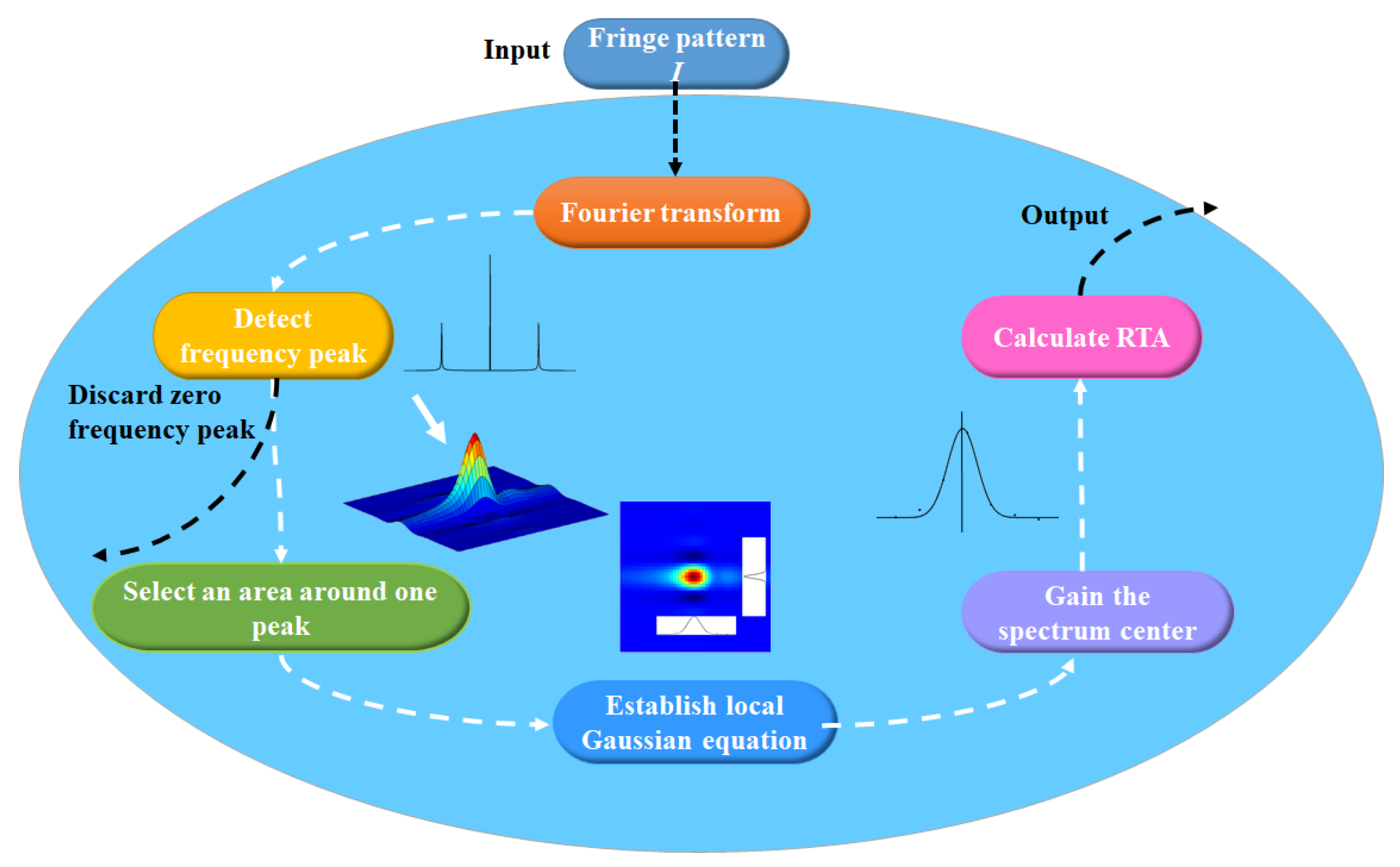
Figure 2 shows the flowchart of the RTA evaluation method. To describe the detailed measures of LGF, the specific steps are included in the following:

Step 1: Carry out fast FT on the intensity distribution I in Equation (5) and detect the frequency peaks on the SSP in Equation (6) by searching the point with the maximum value with the value depressed at the original point.

Step 2: Mark the points detected as (−u₀, −v₀) and (u₀, v₀), and keep the number order of these points (m₀, n₀).

Step 3: Choose a small area with certain FPs around (−u₀, −v₀) or (u₀, v₀) and store the values of these spectrum pixels in this small area. Divide the little area and mesh it into a new grid, so the computational grid size becomes smaller. Correspondently, Δu and Δv are represented as Δu_l and Δv_l, respectively, in this small area.

Step 4: Fit the spectra values in the small piece by the Gaussian formula in Equation (10) and the known values stored in step 3. Calculate the new spectrum coordinates (−u_0l, −v_0l) or (u_0l, v_0l) of the peak tip in the more refined grid by Equation (11).

Step 5: Calculate the RTA by Equation (13) with the coordinates (u_0l, v_0l) found in step 4.

The steps in Figure 2 can also be understood by referring to the description above and the output of it represents RTA values improved.

3. Numerical Simulations

To investigate the performance of the local fitting effects of our method in detail, a series of numerical simulations are carried out, and some RTA retrieving results are given. In these simulations, three cases with different simulated objects are introduced to check the applicability of the proposed method.

In the first case, the configuration [26] reported before is used to detect RTA and improve the precision of the RTA calculation. In this circumstance, the other fringe by the interference of two plane waves is used to avoid the disturbance of another object spectrum so that the effects of the method can be observed more thoroughly and carefully. For comparison, the RTA searching results by direct searching method (DSM) without any more operations, local cubic spline interpolation (LCSI), and Local quintic polynomial fitting (LQPF) are also studied in this work.

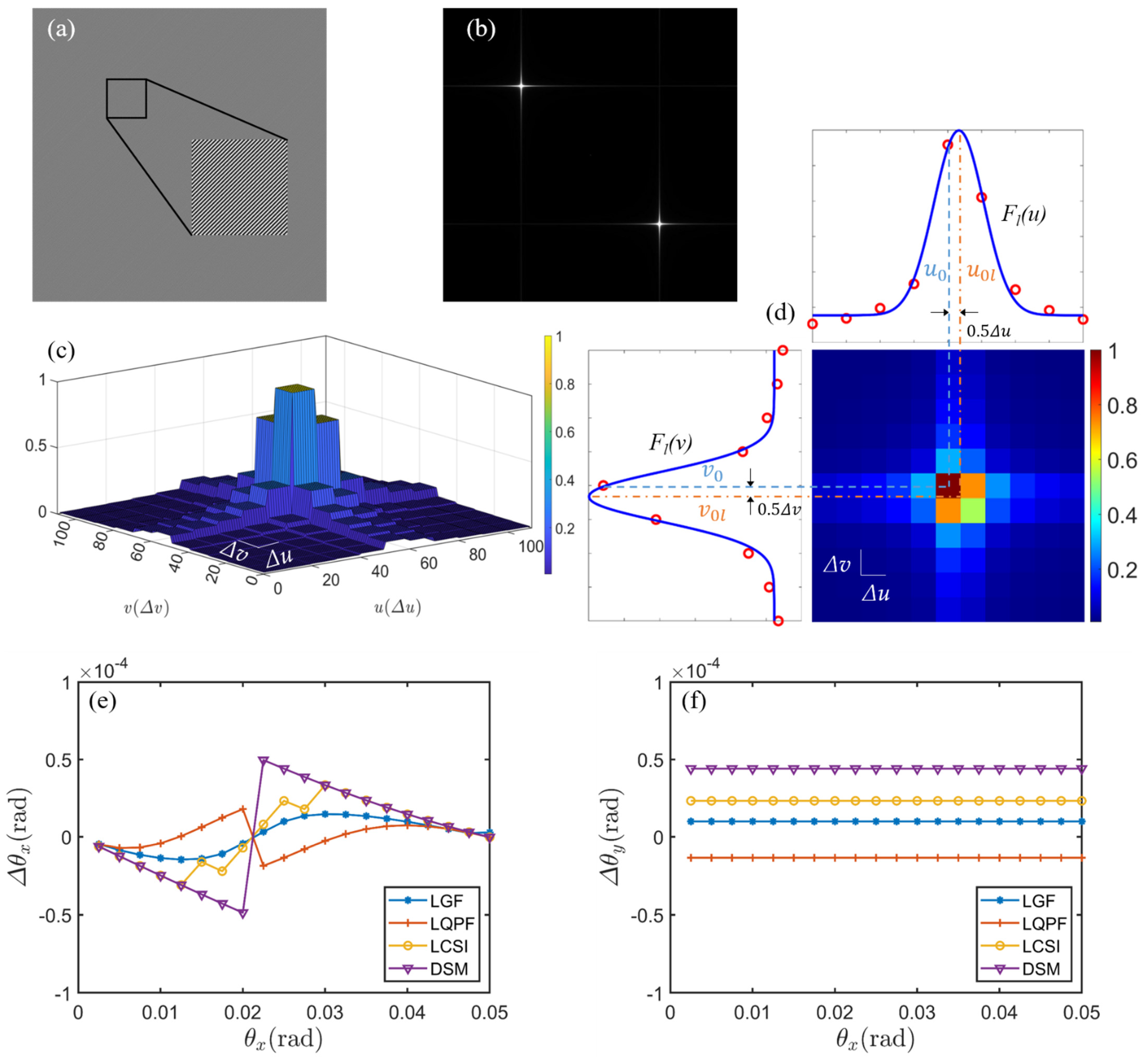
During the simulation, there are 1024 × 1024 pixels with 5 μm × 5 μm size on the CCD recording chip and the recording distance is set to be z = 48 mm to satisfy the requirement of the sampling theory [11]. The laser source with the wavelength of λ = 532 nm is used as the illumination. To exclude the interference of other factors, the configuration is equipped with another CCD2 to record the fringes carrying the reference tilt information [26]. The real amplitudes of the two plane waves are equal and the tilt angle of one plane wave is set to be smaller than 0.05 rad (about 3 degrees which is always used in digital holography) across x and y directions. The interference fringes on the CCD2 recording plane are shown in Figure 3a. Figure 3b gives the spectrum distribution from the Fourier transform of Figure 3a with the zero frequency spectrum depressed. The two delta functions in Equation (6) are obvious since there is no disturbance from other objective spectra. The spectra distribution in adjacent ten Δus and ten Δvs around one delta function center on the SSP is drawn in Figure 3c, where the spectra distributions are discrete, and the values are averaged in one unit Δu × Δv. The curves for these distributions in two directions are plotted in Figure 3d, where the center (u₀, v₀) of the frequency peak before fitting deviates from the fitted Gaussian function center (u_0l, v_0l) and the maximum offset is (0.5Δu, 0.5Δv). Because the fast Fourier transform and other factors incur diffusion, neither of the two curves is a theoretical delta function but a distribution similar to the Gaussian function. So the Gaussian function is chosen for fitting as analyzed before. To fit the spectra distribution, the small area around point (u₀, v₀) is enmeshed again with a smaller grid of 0.2Δu and 0.2Δv. A target Gaussian function is established in the computer and the new function center (u_0l, v_0l) is determined by Equation (11), and then, RTAs are calculated by Equation (13). By recording theory and applications in digital holography, RTA values should be smaller than the value of λ/(2Δx) and λ/(2Δy), which is about 0.05 rad in the simulation conditions here. Considering this selectable scope, to investigate the performance of the method in the practice applications, 20 RTAs are chosen from 0.0025 rad to 0.05 rad with intervals of 0.0025 rad and corresponding errors are calculated by DSM. Meanwhile, the calculation results from Equation (13), interpolation method, and polynomial method are also carried out for comparison. The errors are calculated by the subtraction of the preset value from the retrieved one of RTA. The error distributions from different methods are shown by four curves in Figure 3e,f. The curves marked by the acronyms of LGF, LQFP, LCSI, and DSM are calculating results from the corresponding methods of local Gaussian fitting, local quintic polynomial fitting, local cubic spline interpolation, and direct searching method, respectively. Figure 3e depicts the calculation results of the errors Δθ_x when θ_x varies from 0.0025 rad to 0.05 rad while θ_y = 0.025 rad. In Figure 3e, the error distribution curve from LGF denoted by symbol ‘−*’ keeps stable and is almost the lowest error value, so the method proposed here performs well. Meanwhile, the LQPF presented by ‘−+’ works slightly worse and LCSI performs slightly poorly. The maximum error for LGF is about 2 × 10⁻⁵ rad, whereas the maximum errors from both interpolation and polynomial fitting reach about 2.5 × 10⁻⁵ rad. The errors in Figure 3f show a similar performance as that in Figure 3e under the same conditions. The trend that the errors Δθ_y do not fluctuate violently with the varying of θ_x shows that the spectra distribution is a function with variable separable as Gaussian function. The maximum value of the tilt angle error by DSM reaches 5 ×10⁻⁵ rad, which conforms to the theoretical prediction. In theory, this threshold value can be calculated by Equation (9) when m₀ or n₀ is replaced by 0.5 under the condition that the spectrum falls at the edge of one FP, which is the worst situation for DSM. The biggest theoretical error is 0.5 × λ/(MΔx) = 5.2 × 10⁻⁵ rad, which is consistent with the simulation results.

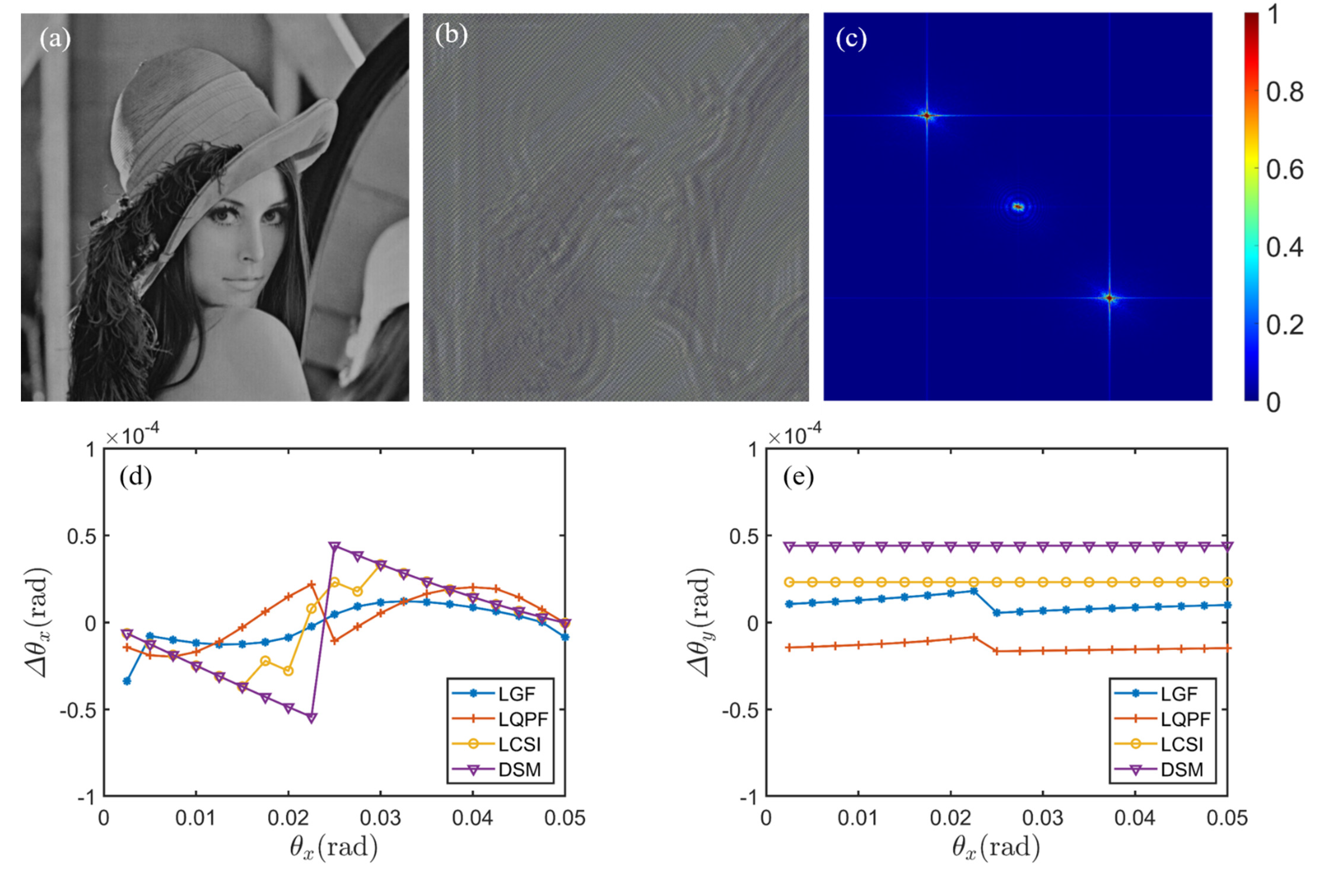
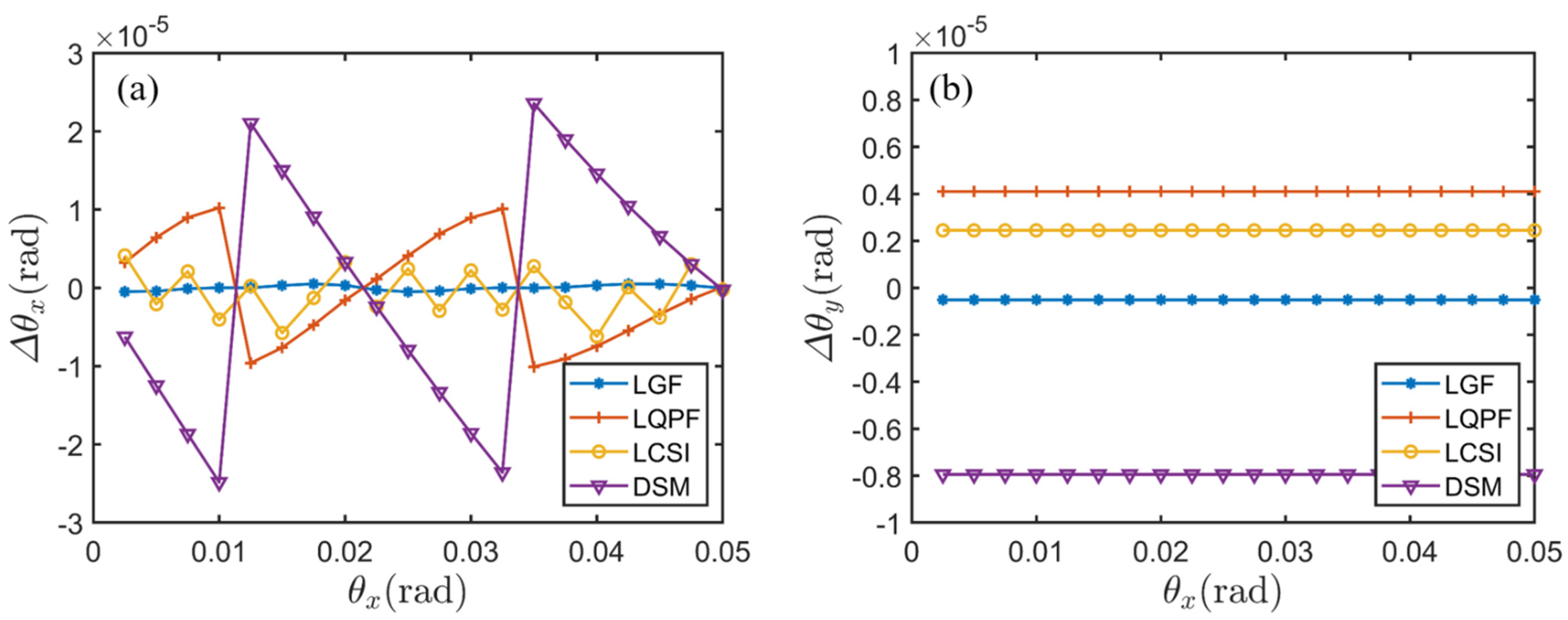
To test the availability of the local fitting method more comprehensively, a portrait figure Lena in Figure 4a is used as the object in the holography recording, and another plane wave is introduced to enhance the zero-frequency component in the objective wave. Both the set up used here and the reconstructed object image have been reported earlier [24]. The amplitudes of the two plane waves are set to be equal and other parameters are similar to the first case in Figure 3. The RTAs are set as θ_x = 0.025 rad and θ_y = 0.025 rad. The same operations are conducted and the results are shown in other sub-figures in Figure 4. Figure 4b is one of the multiplexing interferometry fringes and Figure 4c is its spectra distribution in the Fourier domain. The zero and extreme low frequency spectra are removed for proper display and frequency peak searching. The two spots do not distribute regularly because of the disturbance of the spectra of the portrait, but their maximum centers locate symmetrically about the origin in Figure 4c. The errors from RTA detecting results for varying values of θ_x from 0.0025 to 0.05 rad and θ_y = 0.025 rad are displayed in Figure 4d,e, respectively. The biggest error for θ_x is still 5 × 10⁻⁵ rad by DSM. Although the LQPF and LCSI methods work better for certain θ_x values, the LGF proposed here performs well because the error distribution keeps low and stable, which can ensure the precision of the retrieved value θ_xl and θ_yl.

Although LGF does not perform well for very few specific values of RTA in Figure 4d, the error curve of LGF keeps stable with small values in the full RTA range shown. The root mean square (RMS) of RTA errors in Figure 4d for LGF, LQPF, LCSI, and DSM are 8.6 × 10⁻⁶ rad, 8.6 × 10⁻⁶ rad, 1.9 × 10⁻⁵ rad, and 2.9 × 10⁻⁵ rad, respectively. RMS of the errors in Figure 4e for the same methods are 4.0 × 10⁻⁶ rad, 1.3 × 10⁻⁵ rad, 2.3 × 10⁻⁵ rad, and 4.4 × 10⁻⁵ rad consequently. The results from these RMS calculations show that the LGF methods are more stable than methods LQPF, LCSI, and DSM. It should be noted that the effect of the RTA error on this amplitude image is not easy to observe, but the RTA error affects the location precision and background of the reconstructed image.

To improve the precision of the retrieved RTA, the zero-padding method (ZPM) is used first before local fitting or interpolating. The interferometry fringe in Figure 3 of case one is zero-padded from 1024 × 1024 to 2048 × 2048 pixels. After the Fourier transform, the small area in Figure 3d is further refined from 11 × 11 to 55 × 55 FPs. The preset values of RTA θ_x are chosen from 0.0025 rad to 0.05 rad with the intervals of 0.0025 rad and θ_y is fixed as 0.025 rad. The corresponding errors are shown in Figure 5a,b. Because of the zero-padding, the data array of the interference fringe across one direction is enlarged double and the maximum error should be decreased by half in theory. The errors for θ_x and θ_y in Figure 5a,b exhibit that the biggest error by DSM is about 2.5 × 10⁻⁵ rad and LGF method works best with the LCSI and LQPF following. The RMS of RTA errors in Figure 5a for LGF, LQPF, LCSI, and DSM are 1 × 10⁻⁶ rad, 6.9 × 10⁻⁶ rad, 3.1 × 10⁻⁶ rad, and 1.5 × 10⁻⁵ rad respectively. RMS of the errors for them in Figure 5b are 1.1 × 10⁻⁶ rad, 4.1 × 10⁻⁶ rad, 2.4 × 10⁻⁶ rad, and 7.9 × 10⁻⁶ rad, consequently. From the whole range of the RTA selection scope, the LGF and LCSI methods are more stable than LQPF and DSM with LGF works a little better based on accuracy.

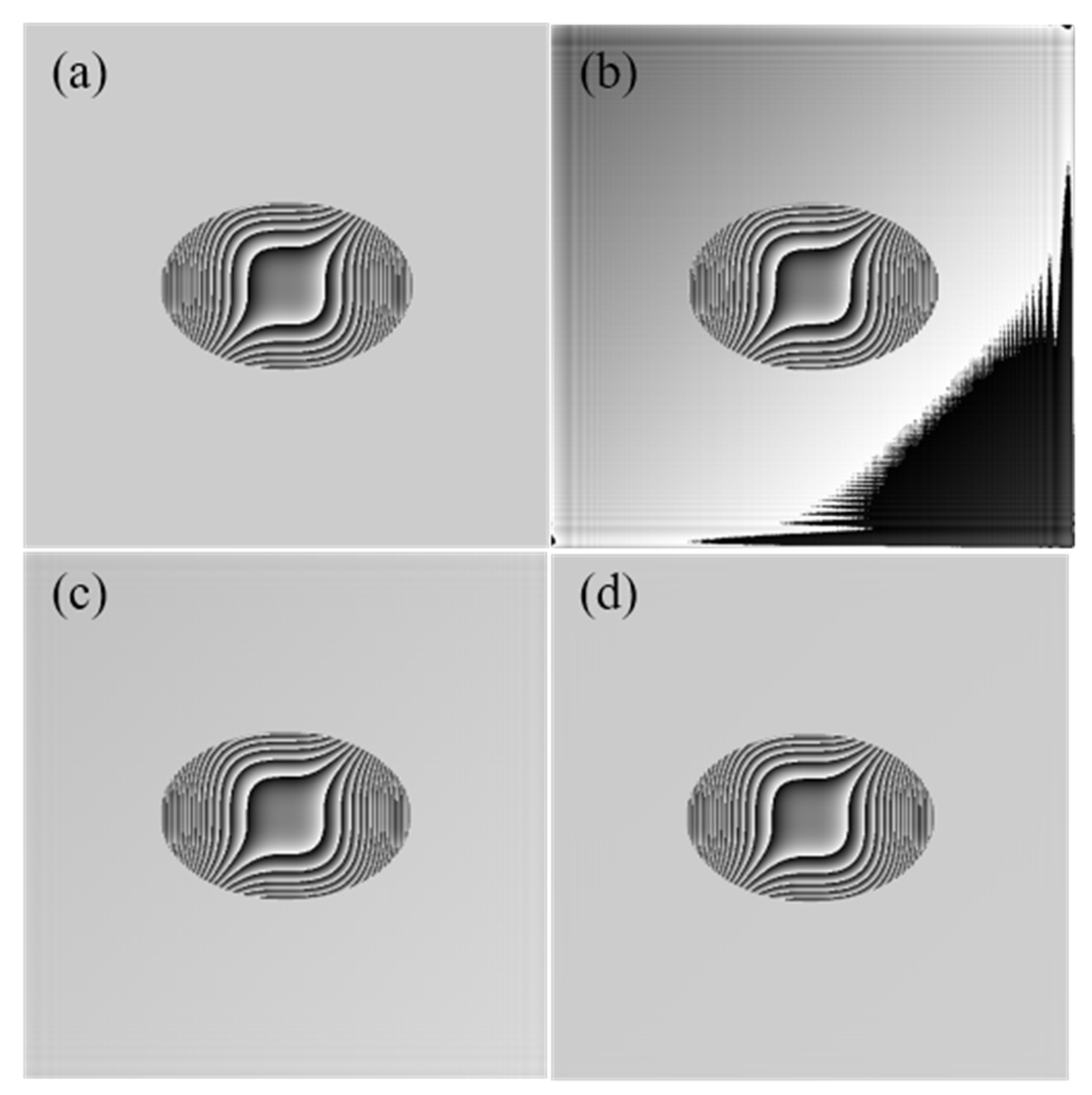
To inspect the effectiveness of RTA precision improving on the imaging quality, a pure phase object with assumed phase in Figure 6a is employed in phase-shifting digital holography (PSDH) simulations with slight RTAs θ_x = θ_y = 0.025 rad. To simulate micro-organism microscopy, there are sharp phase changes in the center area of Figure 6a and the phase around is a constant. The algorithm of the PSDH technique [26] is used to retrieve the object wave on the recording plane, and the RTA values are detected to correct this object wave affected by the reference tilt.

The RTA errors calculated by DSM are Δθ_x = Δθ_y = 4.4 × 10⁻⁵ rad and the object phase is shown in Figure 6b. Because of the RTA error, the reconstructed phase is disturbed by square grid at the edge. Because of the residual RTA error, the lower right corner of Figure 6b tilts up, showing that the constant phase background is spoiled. The errors of RTA by LGF are Δθ_x = Δθ_y = 5 × 10⁻⁶ rad, and the precision is improved by one order of the magnitude. The corresponding phase quality in Figure 6c is also improved considerably. Although the phase map is almost perfect, residual error exists at the edge. To decrease the RTA error further, the ZPM method and LGF are rescued successively to make the retrieved phase distribution better and the RTA errors are reduced to Δθ_x = Δθ_y = 1 × 10⁻⁶ rad. This enhanced precision leads to the high quality of phase distribution in Figure 6d. It should be noted that the RTA computing results by LGF is accurate enough to reconstruct the object phase like that in Figure 6c for the application of biomedical imaging. If the requirement for the phase distribution is not very high in digital holography microscopy, the result in Figure 6c is also acceptable for the phase imaging task. However, for high-quality imaging, higher precision is necessary to detect a more accurate RTA value.

4. Conclusions

A robust RTA evaluation method is proposed by local Gaussian fitting, which can work without increasing the requirement on either the resolution of the recording device or computing hardware. It can take advantage of the redundant information implicated in the neighboring area of the frequency peak on the SSP. The precision of the detected RTA can be improved by one order of amplitude by the proposed method in both off-axis and in-line digital holography to ensure the quality of the reconstructed image. The merits of this technique exhibit in three aspects: the first one is that it can alleviate the requirement on the recording device when the precision of the RTA is improved; the second one is that it relaxes the demand on the large capacity of the ram in computer and can work on computers with a low configuration; the last one is that the method is efficient in the precision improvement because all capacity of the data array hardly increase. It should be noted that the zero-padding method is also an effective method in the improvement of RTA evaluation precision. However, the large data array caused by zero-padding imposes a high requirement on the computer configuration and decreases computation efficiency. This method here is expected to bring convenience and high imaging quality to the DH and super-resolution imaging. It is especially expected to be prosperous in the application of off-axis hologram reconstruction for quantitative phase imaging, where RTA determination needs to be realized with high accuracy.

References

- De Nicola, S.; Ferraro, P. Fourier-transform calibration method for phase retrieval of carrier-coded fringe pattern. Opt. Commun. 1998, 151, 217–221. [Google Scholar] [CrossRef]
- Bone, D.J.; Bachor, H.A.; Sandeman, R.J. Fringe-pattern analysis using a 2-D Fourier transform. Appl. Opt. 1986, 25, 1653–1660. [Google Scholar] [CrossRef]
- Takeda, M.; Ina, H.; Kobayashi, S. Fourier-transform method of fringe-pattern analysis for computer-based topography and interferometry. JosA 1982, 72, 156–160. [Google Scholar] [CrossRef]
- Gustafsson, M.G. Surpassing the lateral resolution limit by a factor of two using structured illumination microscopy. J. Microsc. 2000, 198, 82–87. [Google Scholar] [CrossRef] [PubMed] [Green Version]
- Gustafsson, M.G. Nonlinear structured-illumination microscopy: Wide field fluorescence imaging with the theoretically unlimited resolution. Proc. Natl. Acad. Sci. USA 2005, 102, 13081–13086. [Google Scholar] [CrossRef] [Green Version]
- Lal, A.; Shan, C.; Xi, P. Structured Illumination Microscopy Image Reconstruction Algorithm. IEEE J. Sel. Top. Quantum Electron. 2016, 22, 50–63. [Google Scholar] [CrossRef] [Green Version]
- Min, J.W.; Yao, B.L.; Ketelhut, S.; Engwer, C.; Greve, B.; Kemper, B. Simple and fast spectral domain algorithm for quantitative phase imaging of living cells with digital holographic microscopy. Opt. Lett. 2017, 42, 227–230. [Google Scholar] [CrossRef]
- Zheng, J.J.; Gao, P.; Yao, B.L.; Ye, T.; Lei, M.; Min, J.W.; Dan, D.; Yang, Y.L.; Yan, S.H. Digital holographic microscopy with phase-shift-free structured illumination. Photonics Res. 2014, 2, 87–91. [Google Scholar] [CrossRef]
- Baek, Y.; Park, Y. Intensity-based holographic imaging via space-domain Kramers–Kronig relations. Nat. Photonics 2021, 15, 354–360. [Google Scholar] [CrossRef]
- Huang, Z.; Memmolo, P.; Ferraro, P.; Cao, L. Dual-plane coupled phase retrieval for non-prior holographic imaging. PhotoniX 2022, 3, 3. [Google Scholar] [CrossRef]
- Poon, T.-C.; Liu, J.-P. Introduction to Modern Digital Holography with MATLAB; Cambridge University Press: Cambridge, UK, 2014. [Google Scholar]
- Huang, Z.; Cao, L. High Bandwidth-Utilization Digital Holographic Multiplexing: An Approach Using Kramers–Kronig Relations. Adv. Photonics Res. 2022, 3, 2100273. [Google Scholar] [CrossRef]
- Liu, C.; Liu, Z.G.; Bo, F.; Wang, Y.; Zhu, J.Q. Super-resolution digital holographic imaging method. Appl. Phys. Lett. 2002, 81, 3143–3145. [Google Scholar] [CrossRef]
- Diouf, M.; Lin, Z.; Harling, M.; Toussaint, K.C. Demonstration of speckle resistance using space–time light sheets. Sci. Rep. 2022, 12, 14064. [Google Scholar] [CrossRef] [PubMed]
- Diouf, M.; Harling, M.; Yessenov, M.; Hall, L.A.; Abouraddy, A.F.; Toussaint, K.C. Space-time vector light sheets. Opt. Express 2021, 29, 37225–37233. [Google Scholar] [CrossRef]
- Yamaguchi, I.; Zhang, T. Phase-shifting digital holography. Opt. Lett. 1997, 22, 1268–1270. [Google Scholar] [CrossRef]
- Zhang, J.Y.; Ren, Y.J.Z.; Zhu, Q.; Lin, Z.Q. Phase-shifting lensless Fourier-transform holography with a Chinese Taiji lens. Opt. Lett. 2018, 43, 4085–4087. [Google Scholar] [CrossRef]
- Liu, H.; RV, V.; Ren, H.; Du, X.; Chen, Z.; Pu, J. Single-Shot On-Axis Fizeau Polarization Phase-Shifting Digital Holography for Complex-Valued Dynamic Object Imaging. Photonics 2022, 9, 126. [Google Scholar] [CrossRef]
- Jung, M.; Jeon, H.; Lim, S.; Hahn, J. Color Digital Holography Based on Generalized Phase-Shifting Algorithm with Monitoring Phase-Shift. Photonics 2021, 8, 241. [Google Scholar] [CrossRef]
- Ma, Z.; Yang, Y.; Zhai, H.; Chavel, P. Spatial angular multiplexing for enlarging the detected area in off-axis digital holography. Opt. Lett. 2013, 38, 49–51. [Google Scholar] [CrossRef]
- Singh, M.; Khare, K.; Jha, A.K.; Prabhakar, S.; Singh, R.P. Accurate multipixel phase measurement with classical-light interferometry. Phys. Rev. A 2015, 91, 021802. [Google Scholar] [CrossRef]
- Tahara, T.; Shimozato, Y.; Awatsuji, Y.; Nishio, K.; Ura, S.; Matoba, O.; Kubota, T. Spatial-carrier phase-shifting digital holography utilizing spatial frequency analysis for the correction of the phase-shift error. Opt. Lett. 2012, 37, 148. [Google Scholar] [CrossRef] [PubMed]
- Li, J.L.; Su, X.Y.; Su, H.J.; Cha, S.S. Removal of carrier frequency in phase-shifting techniques. Opt. Lasers Eng. 1998, 30, 107–115. [Google Scholar] [CrossRef]
- Xu, X.F.; Wang, X.W.; Wang, H. Accurate Image Locating by Hologram Multiplexing in Off-Axis Digital Holography Display. Appl. Sci. 2022, 12, 1437. [Google Scholar] [CrossRef]
- Xu, X.F.; Ma, T.Y.; Jiao, Z.Y.; Xu, L.; Dai, D.J.; Qiao, F.L.; Poon, T.-C. Novel Generalized Three-Step Phase-Shifting Interferometry with a Slight-Tilt Reference. Appl. Sci. 2019, 9, 5015. [Google Scholar] [CrossRef] [Green Version]
- Xu, X.F.; Zhang, Z.W.; Wang, Z.C.; Wang, J.; Zhan, K.Y.; Jia, Y.L.; Jiao, Z.Y. Robust digital holography design with monitoring setup and reference tilt error elimination. Appl. Opt. 2018, 57, B205–B211. [Google Scholar] [CrossRef]
- Dai, M.J.; Wang, Y. Fringe extrapolation technique based on Fourier transform for interferogram analysis. Opt. Lett. 2009, 34, 956. [Google Scholar] [CrossRef]
- Du, Y.Z.; Feng, G.Y.; Li, H.R.; Zhou, S.H. Accurate carrier-removal technique based on zero padding in Fourier transform method for carrier interferogram analysis. Optik 2014, 125, 1056–1061. [Google Scholar] [CrossRef]
- Xu, J.; Xu, Q.; Peng, H. Spatial carrier phase-shifting algorithm based on least-squares iteration. Appl. Opt. 2008, 47, 5446–5453. [Google Scholar] [CrossRef]
- Gu, L.; Li, Y.; Zhang, S.; Zhou, M.; Xue, Y.; Li, W.; Xu, T.; Ji, W. Molecular-scale axial localization by repetitive optical selective exposure. Nat. Methods 2021, 18, 369–373. [Google Scholar] [CrossRef]
Figure 1.
Gaussian function and spectra distribution on an SSP (a) a Gaussian distribution in the spatial domain (b) one of the frequency peaks in the Fourier spectra domain.
Figure 2.
Flowchart for the robust RTA evaluation method.
Figure 3.
Analysis of one frequency peak on spatial spectrum plane and comparison of the result from LGF with that from other RTA evaluation methods (a) interference fringe by two plane waves (b) one frequency spectrum distribution on SSP (c) three-D frequency spectrum distribution and (d) error source for the location of one frequency peak center, (e) Δθx and (f) Δθy distributions from four methods when θy = 0.025 rad.
Figure 4.
Spectra distribution of one real hologram and comparison of the result from LGF with that from other RTA evaluation methods (a) original object (b) hologram (c) corresponding spectrum distribution. (d) Δθx and (e) Δθy distributions from four methods when θy = 0.025 rad.
Figure 5.
Comparison of the result from LGF with that from other RTA evaluation methods after zero-padding operation. (a) Δθx and (b) Δθy distributions from four methods when θy = 0.025 rad.
Figure 6.
Phase object reconstruction results with different RTA errors (a) Ground truth, and by (b) DSM method, (c) LGF method, (d) LGF with ZPM.
Publisher’s Note: MDPI stays neutral with regard to jurisdictional claims in published maps and institutional affiliations. |
© 2022 by the authors. Licensee MDPI, Basel, Switzerland. This article is an open access article distributed under the terms and conditions of the Creative Commons Attribution (CC BY) license (https://creativecommons.org/licenses/by/4.0/).
Share and Cite
MDPI and ACS Style
Xu, X.; Wang, H.; Sheng, H.; Luo, W.; Wang, X. Robust Evaluation of Reference Tilt in Digital Holography. Appl. Sci. 2022, 12, 11224. https://0-doi-org.brum.beds.ac.uk/10.3390/app122111224
AMA Style
Xu X, Wang H, Sheng H, Luo W, Wang X. Robust Evaluation of Reference Tilt in Digital Holography. Applied Sciences. 2022; 12(21):11224. https://0-doi-org.brum.beds.ac.uk/10.3390/app122111224
Chicago/Turabian StyleXu, Xianfeng, Hao Wang, Hui Sheng, Weilong Luo, and Xinwei Wang. 2022. "Robust Evaluation of Reference Tilt in Digital Holography" Applied Sciences 12, no. 21: 11224. https://0-doi-org.brum.beds.ac.uk/10.3390/app122111224
Note that from the first issue of 2016, this journal uses article numbers instead of page numbers. See further details here.