
Low-Photon Counts Coherent Modulation Imaging via Generalized Alternating Projection Algorithm

1
Hebei Key Laboratory of Power Internet of Things Technology and the Department of Electronics and Communication Engineering, North China Electric Power University, Baoding 071003, China
2
Shenzhen Key Laboratory of Robotics Perception and Intelligence and the Department of Electrical and Electronic Engineering, Southern University of Science and Technology, 1088 Xueyuan Avenue, Shenzhen 518055, China
3
Department of Mechanical Engineering, Massachusetts Institute of Technology, 77 Massachusetts Ave, Cambridge, MA 02139, USA
4
Singapore-MIT Alliance for Research and Technology (SMART) Centre, 1 Create Way, Singapore 117543, Singapore
5
Singapore-MIT Alliance for Research and Technology (SMART) Centre, 1 Create Way, Washington, DC 20036, USA
*
Author to whom correspondence should be addressed.
†
These authors contributed equally to this work.
Appl. Sci. 2022, 12(22), 11436; https://0-doi-org.brum.beds.ac.uk/10.3390/app122211436
Submission received: 30 July 2022
/
Revised: 7 September 2022
/
Accepted: 12 September 2022
/
Published: 11 November 2022
(This article belongs to the Special Issue Holography, 3D Imaging and 3D Display Volume II)
Abstract
:Phase contrast imaging is advantageous for mitigating radiation damage to samples, such as biological specimens. For imaging at nanometer or atomic resolution, the required flux on samples increases dramatically and can easily exceed the sample damage threshold. Coherent modulation imaging (CMI) can provide quantitative absorption and phase images of samples at diffraction-limited resolution with fast convergence. When used for radiation-sensitive samples, CMI experiments need to be conducted under low illumination flux for high resolution. Here, an algorithmic framework is proposed for CMI involving generalized alternating projection and total variation constraint. A five-to-ten-fold lower photon requirement can be achieved for near-field or far-field experiment dataset. The work would make CMI more applicable to the dynamics study of radiation-sensitive samples.
1. Introduction
The past 20 years saw the rapid advance of coherent diffraction imaging (CDI) techniques [1,2,3]. CDI disposes of the imaging lens and its theorical resolution is only determined by the wavelength of illumination radiation and the maximum angles that the diffracted light can be reliably detect. CDI is suitable for any coherent radiations, including synchrotron X-rays [4,5,6] or pulsed free electron lasers X-rays [7] and cold emission electron beams [8]. Various variants of algorithms, mostly derived from the Gerchberg–Saxton (GS) and the Fienup algorithm [9,10,11,12,13], were proposed. The oversampling smoothness algorithm in [9] properly introduces a spatial frequency filter based on the hybrid input–output (HIO) [3]. This algorithm makes full use of the smooth constraint of the region outside the support in the iterative process, and is proven to be robust when there is Poisson noise in the diffraction pattern. Single-shot CDI, however, requires isolated samples, and the sample phase variation is also restricted [14,15].
Ptychography ameliorates the drawbacks of CDI by recording multiple diffraction patterns with illumination overlapping. Ptychography became a main imaging modality at synchrotron facilities worldwide [15,16,17,18,19,20,21,22,23,24], and also gained popularity in the electron microscopy community [24,25,26,27]. In the presence of the noise of light and detectors, some optimization frameworks are proposed for ptychography and an order of magnitude of reconstruction quality is achieved by combining the conjugate gradients with preconditioning strategies, as well as regularization accounting for the statistical noise model of real experiments [28,29].
For imaging of biological samples, the ultimate limit of resolution is set by the radiation damage, and thus the performance of the imaging method under low illumination flux is essential [30,31,32,33]. Previous researchers also demonstrated that electron ptychography is a promising phase-contrast imaging technique with the advantage of high dose efficiency [30,34,35,36]. According to the dose factorization theorem [37], there is a strong hope that ptychography can keep its high performance under low light conditions. Using two-dimensional MoS2 crystal samples, it was demonstrated that highly quantitative phase can be obtained under low electron dose conditions [34].
The requirement of multiple measurements in ptychography makes it unsuitable for fast sample dynamics investigation. CMI is an alternative solution in addressing the weakness of CDI, but in a single-shot manner [38,39]. In CMI, a modulator is placed between the object and the detector to strengthen the coding of the phase of diffracted waves in a diffraction pattern. CMI is shown to work well under illumination flux greater than photons. Nevertheless, collected diffraction patterns can be severely interfered by Poisson noise as the illumination weakens, which affects the stability and accuracy of the algorithm. Therefore, it is worthy of retrieving phase information from contaminative diffraction patterns in biological specimens with efficient algorithm and ideal illumination photons. For lower flux, the current algorithm starts to encounter convergence difficulty and image artifacts in reconstruction. Recently, the PhENN neural network was proposed to improve the low-flux performance of CDI [40], as well as CMI [41]. Their training requirement can be computationally expensive and still there is concern about their suitability on general samples. Untrained learning methods also exist [42], but they are yet to be demonstrated for the low photon scenario.
In this manuscript, we report a computationally efficient and robust algorithm, based on generalized alternating projections (GAP), that preserves the advantages of CMI to recover the phase information from low signal-to-noise ratios data. GAP consists of two sub-problems, including measurement formation and statistical prior regularization. The paper is organized as follows: Section 2 details the theory and metric of the proposed method. In Section 3, the results and quantitative analysis of the simulation are presented. Experimental results of visible light and X-rays are described in Section 4 before a summary of our method is drawn in Section 5.
2. Methods
Generally, phase retrieval is a non-convex optimization problem, due to the intensity measurement of wavefields. Unlike convex situations, non-convex optimization problems are at risk of stagnation at local minima and saddle points [43]. Current phase retrieval algorithms usually introduce additional regularizing priors to the optimization function to reduce the scope of the solution space.
In the following, we briefly sketch the basics of the proposed CMI-GAP algorithm. As is common in machine learning [44], dictionary learning [45], compressive sensing [46], as well as sparse coding [47], the phase retrieval problem in CDI can be represented as an objective function
Here, is the complex object wavefield to be recovered. is the measured diffraction data. stands for the free space propagation operator. In the near-field, forward propagation is defined as
is the transmission function of the modulator and is the support function. denotes the angular spectrum propagation method. Additionally, in far-field, forward propagation is defined as
where denotes the Fourier transform.
In Equation (1), is a smooth fidelity term, which can be minimized under a standard gradient descent method, while is a non-differentiable regularization term. The proximal gradient algorithm can be adopted for such optimization problems; the so-called proximal operator is defined as
The phase solution x is calculated by minimizing the combination of the fidelity term and regularization term . Constant adjusts the weighting of the regularization term relative to the fidelity term.
Iterative phase retrieval algorithms for CDI involve projections between two spaces and imposition of constraints, which can generate satisfying results under certain limitations [48]. For CMI, the propagation operator also includes wavefront modulation. We observed that a forward operator with a complex matrix structure could enhance the encoding effectiveness of the sample phase and accelerate the retrieval process greatly. CMI shows good performance in X-ray and optical experiments when the measured data are not subject to heavy noise [38,39].
The GAP framework is one popular method that can retrieve high fidelity images from contaminated data by incorporating sample priors. Compared with other algorithms, such as ADMM [49] and TwIST [50], the GAP algorithm uses only Euclidean projection in updating the unknown . PnP-GAP exhibits global convergence for data recorded in the scheme of snapshot compressive imaging [51,52].
In this work, we adopt the GAP strategy to suppress the noise and enhance the performance of CMI in a low lighting scenario. According to the GAP framework, Equation (4) can be reformulated as
Here, a new variable is introduced into the objective function. The conditional constraint term is then replaced with a penalty term, given by
where and are the variables that need to be optimized. The optimum may be effectively reached by updating and in an alternating fashion. In updating , we are inclined to get more information from the diffraction pattern to form the wavefront; while in updating z, the resultant is conditioned to fit more accurately with the real samples. The specific details of implementation are as follows:
Updating : assume is fixed, Equation (6) can be simplified to
and be solved as
Updating : assume is fixed and the total variation (TV) regulation, Equation (6) can be rewritten as
The TV regulation term features a good edge-preserving property, and Equation (9) forms a denoiser. The anisotropic TV defined as
was used in this work, and the accelerated implementation method in [53] was adopted. The symbols and denote the first derivatives along the horizontal and vertical directions, respectively.
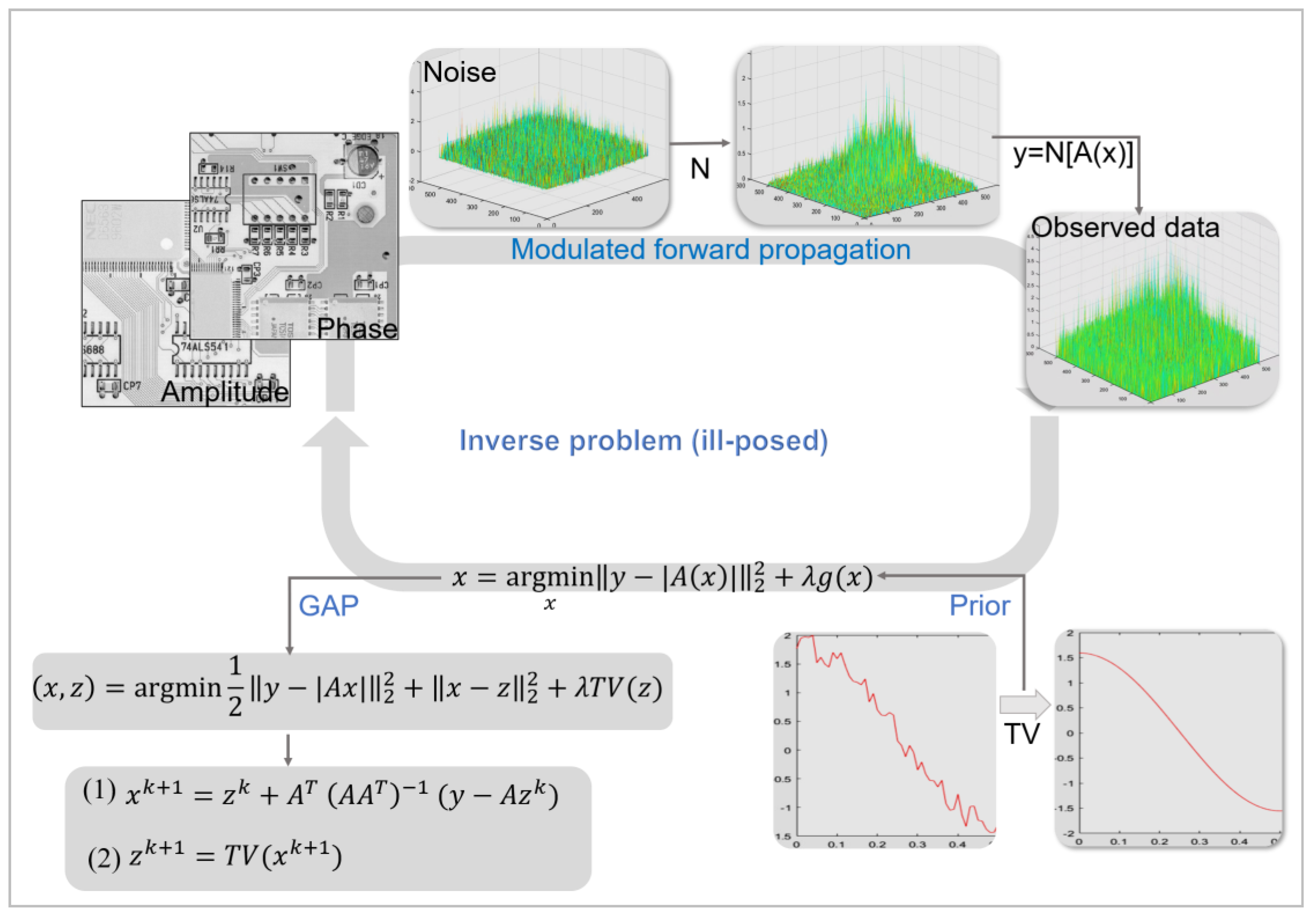
Figure 1 shows the overall flowchart of the CMI-GAP algorithm.
Both numerical simulations and optical experiments with similar parameters were carried out to evaluate the performance of the proposed algorithm. For both cases, the image quality was quantitively evaluated via root-mean-square (RMS) [54],
where denotes the reconstructed wavefront, denotes the ground truth, denotes the Fourier transform operator. The peak signal-to-noise ratio (PSNR) was also used.
3. Numerical Simulations
In this section, simulations with a different number of illumination photons and experiment settings are presented. The sample illumination was formed by a 1.5 mm pinhole irradiated by a collimated 632.8 laser beam. Images of printed circuit boards were used for sample amplitudes and phases. The code was written with MATLAB and run on a computer equipped with 16 GB RAM and a GTX1060 6 GB GPU.
3.1. Near-Field Simulation
The convergency requirement of the CMI method determined other distance parameters; a large sample (pinhole) to modulator distance increases the effectiveness of the support constraint but at the cost of degraded image resolution in the reconstruction. A value between 20 and 40 mm was found to give the best balance. Therefore, the separations between the sample, modulator, and detector were set to mm and mm according to our experimental settings. Wave propagation between the three planes was calculated with the angular spectrum algorithm. The sampling intervals were 5.04 mm at all planes.
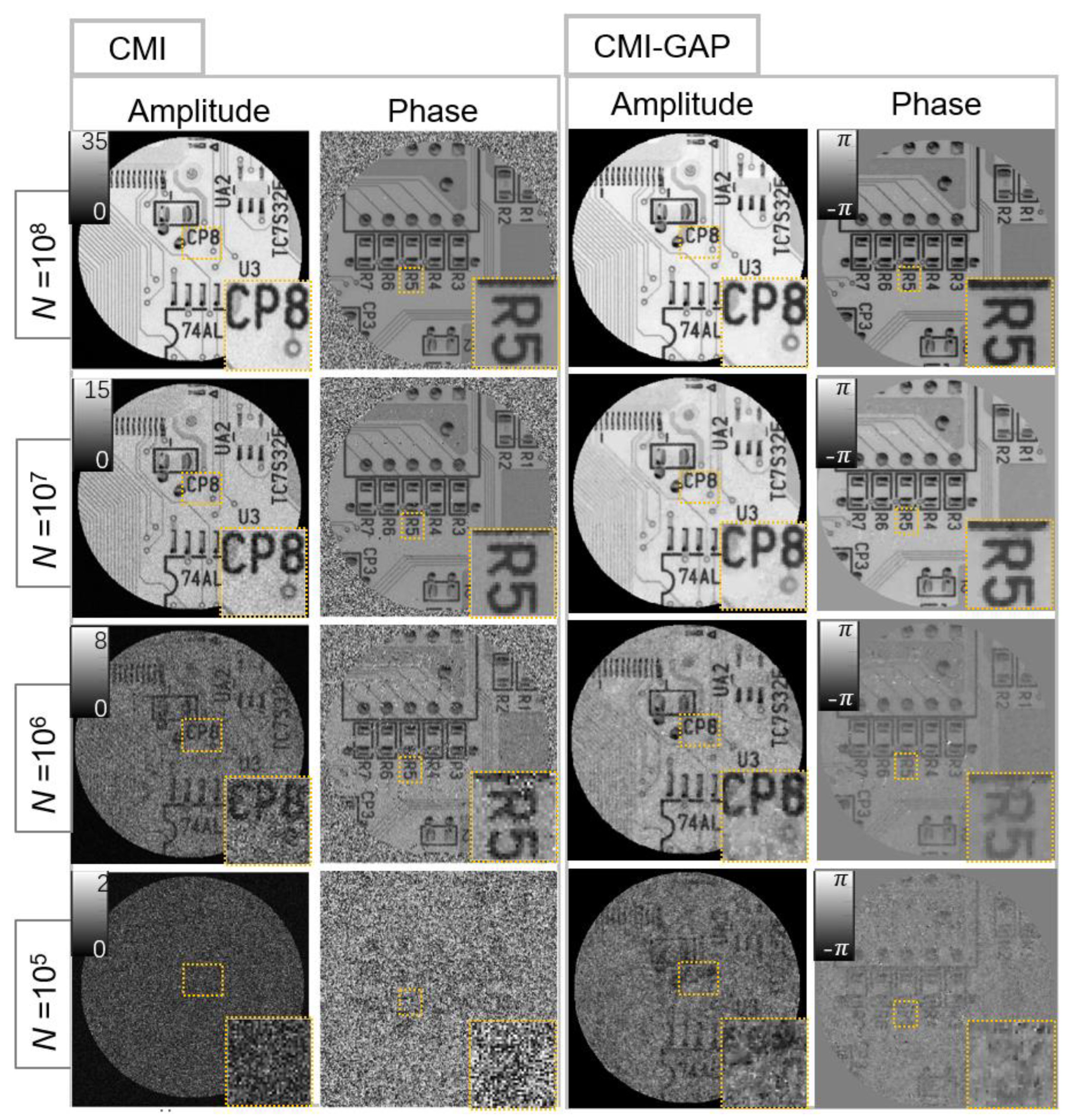
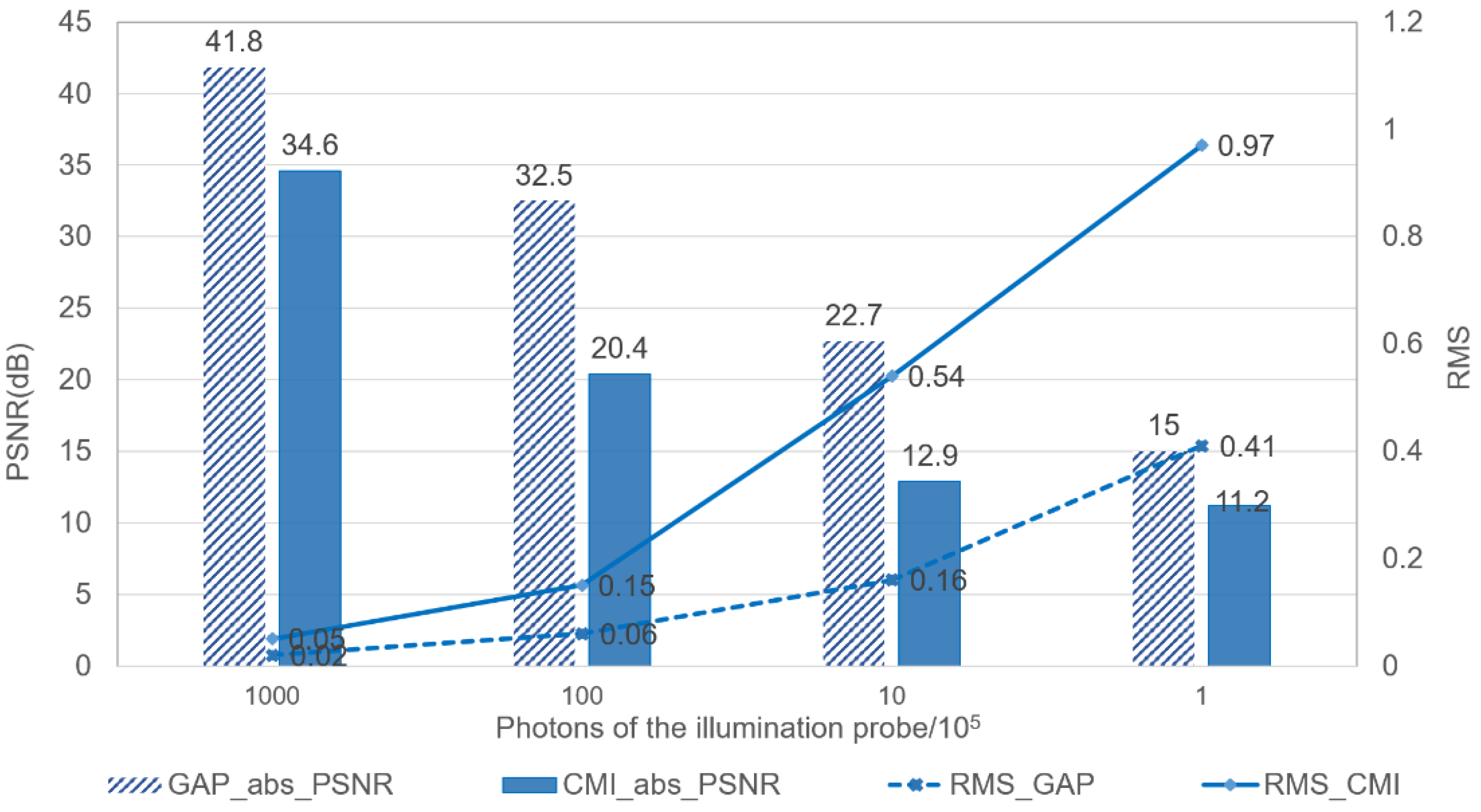
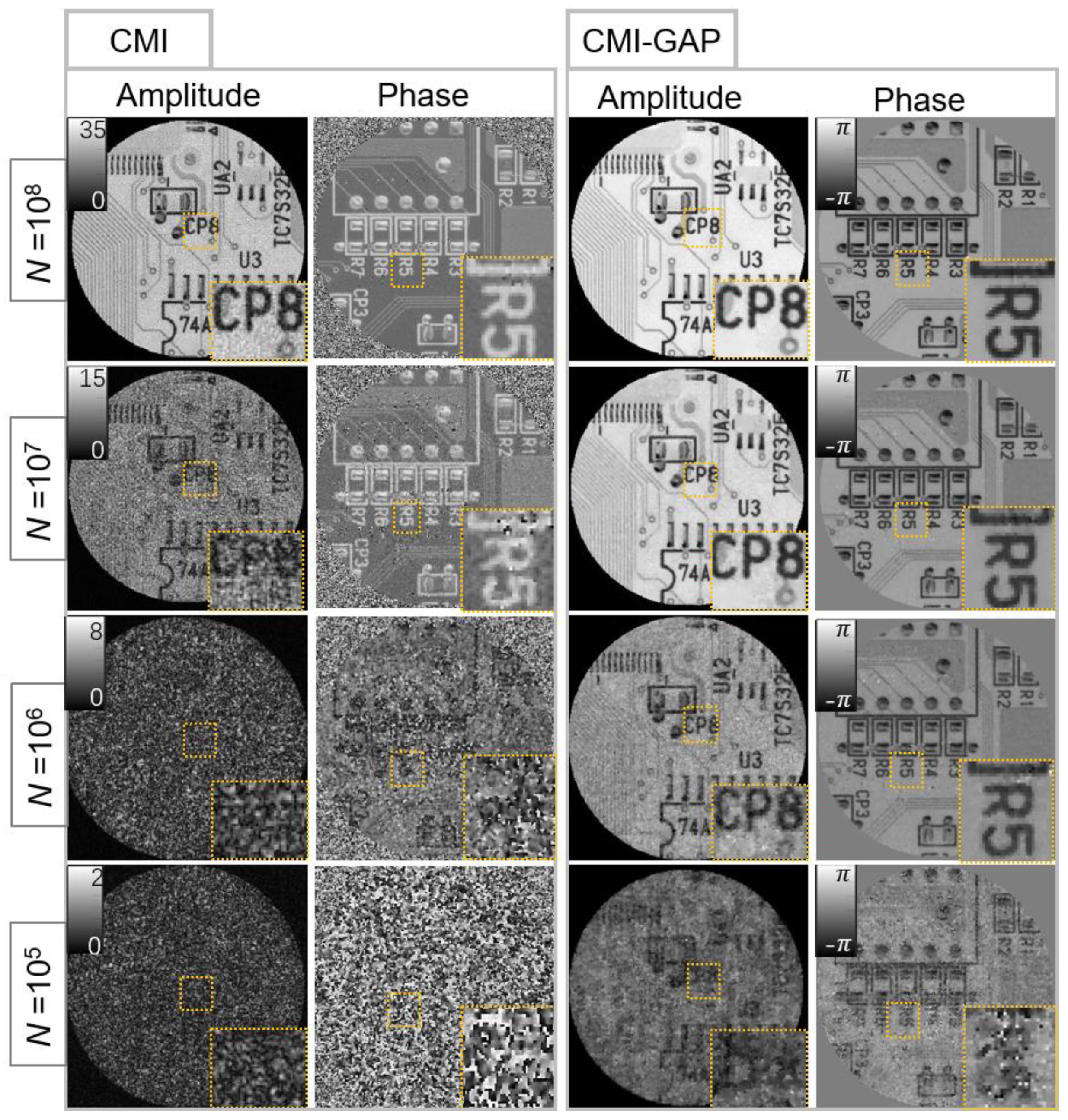
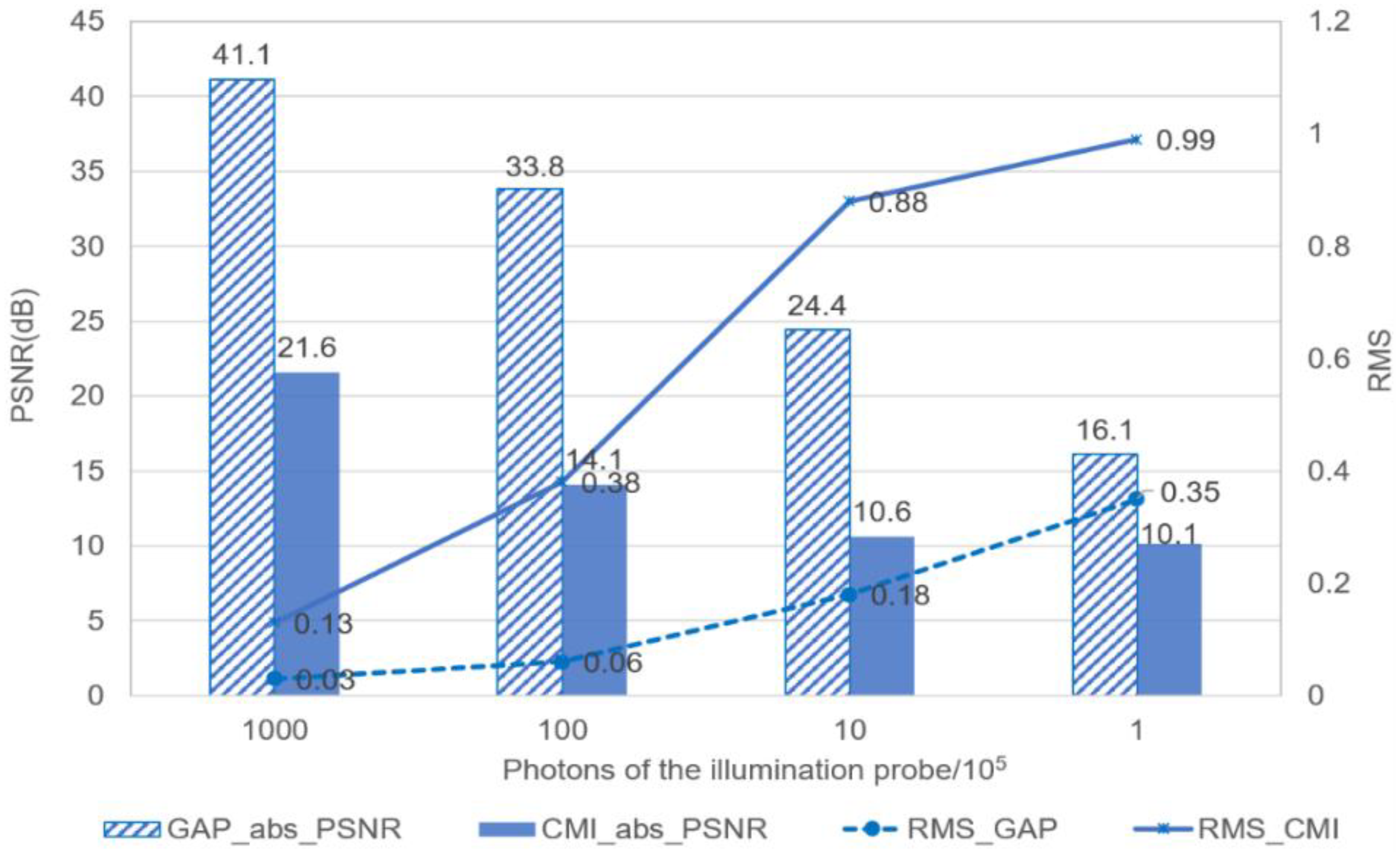
The performance of CMI-GAP was evaluated with the illumination photon number of being . Reconstructed object amplitudes and phases, as well as the PSNR and RMS, are shown in Figure 2 and Figure 3, respectively. The iteration number of the traditional algorithm is about 500 and 50 with CMI-GAP. Overall, one can see the CMI-GAP algorithm shows better performance than CMI. When is above , their reconstruction quality is comparable; as decreases, the RMS curve of CMI increases rapidly. When drops below , the CMI-GAP algorithm can still retrieve details in most of the regions.
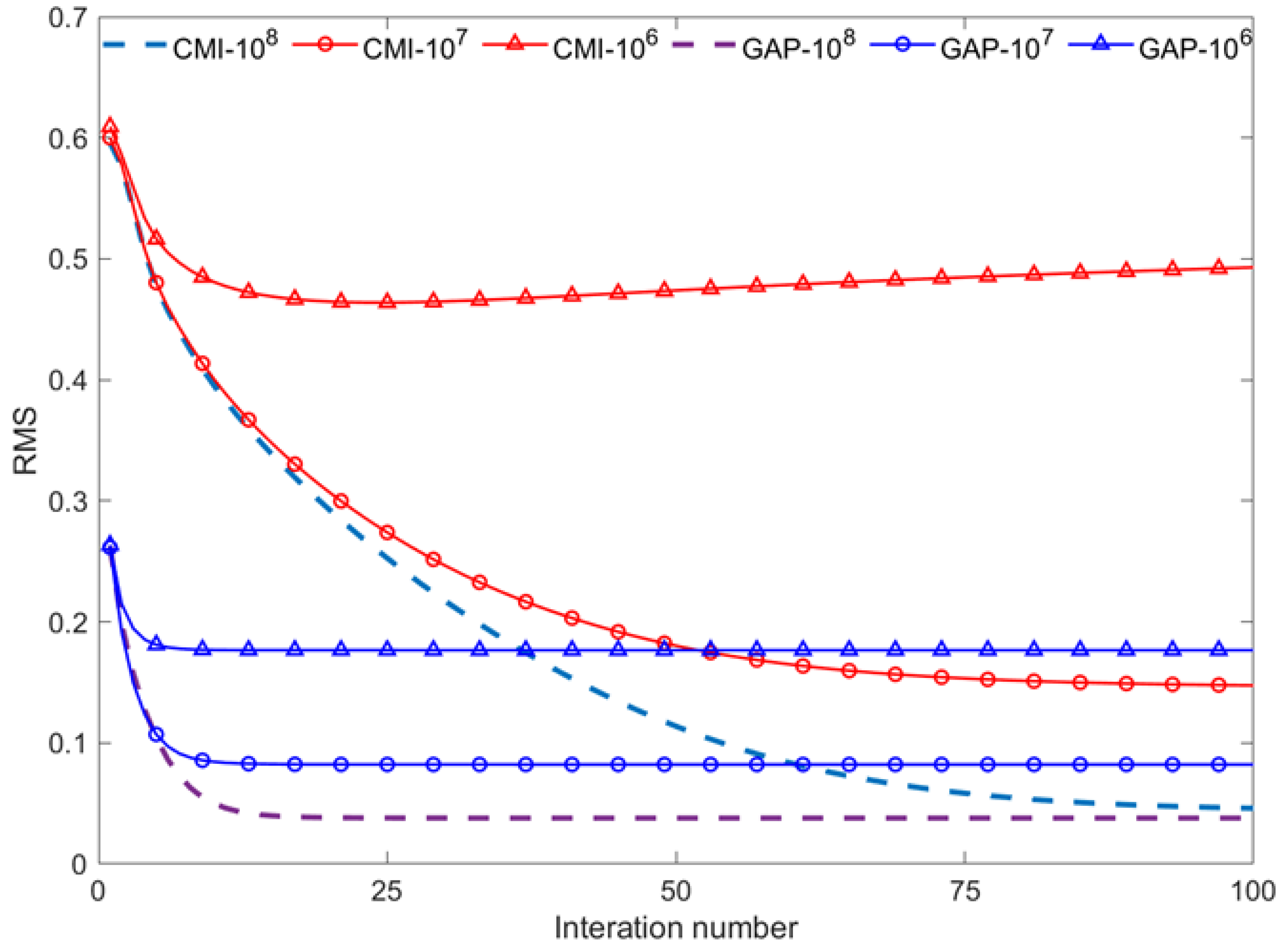
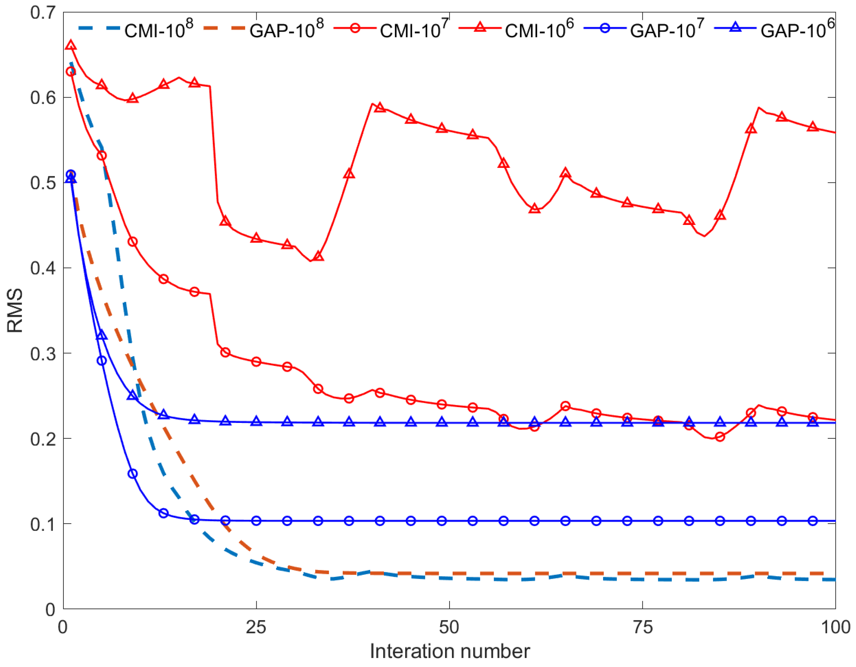
The convergence rate dependence of the CMI-GAP algorithm on the illumination photons was then studied. Figure 4 shows the comparison of the convergence rate for the photon counts of , , and . Notably, the proposed algorithm converges rapidly in the first ten iterations when the number of photons is . The RMS value reaches 0.08 before it stagnates, while the RMS using the CMI algorithm converges relatively slowly and reaches an RMS of 0.15 after 30 iterations. As decreases further, the performance difference between the two algorithms becomes more apparent.
3.2. Far-Field Simulation
We also validated the effectiveness of the CMI-GAP algorithm for the far-field geometry. In the simulations, a laser source was assumed. The sample to modulator distance was . The modulator was placed on the front focal plane of a Fourier transform lens with a focal length of . At the back focal plane of the lens, the detector was located.
Reconstructed amplitudes and phases are shown in Figure 5. Figure 6 shows the RMS and PSNR against the illumination photon numbers of . The iteration number of the traditional algorithm is about 500 and 50 with CMI-GAP. A clear deviation in the image quality can be seen when is below similar to the near-field case. In contrast, CMI-GAP produces significant enhancement in reconstruction quality, with as much as 20 dB and three times improvement in PSNR and RMS, respectively. The RMS bears a similar behavior as the near-field geometry. Figure 7 demonstrates the convergence curve when are and . Generally speaking, the CMI-GAP algorithm has a relatively low RMS value and a faster convergence. The vibration of the convergence curve of the CMI algorithm was due to the algorithm switching, i.e., the HIO and DM algorithm are switched at specified iterations to promote convergence.
4. Verification with Experimental Data
Optical experiments were performed to verify the CMI-GAP algorithm in a low light flux scenario. A stabilized 632.8 He-Ne laser was used to form a quasi-monochromatic and collimated illumination beam. The sample was a positive USAF resolution target stuck on a hole. Scattered waves from the sample were modulated by a downstream thin modulator. An sCMOS camera (Thorlabs CS2100) with a pixel size of 5.04 was used to collect the diffraction data. A ptychography dataset was recorded with an illumination probe flux of photons. The retrieved modulator will be used in our CMI and CMI-GAP reconstruction.
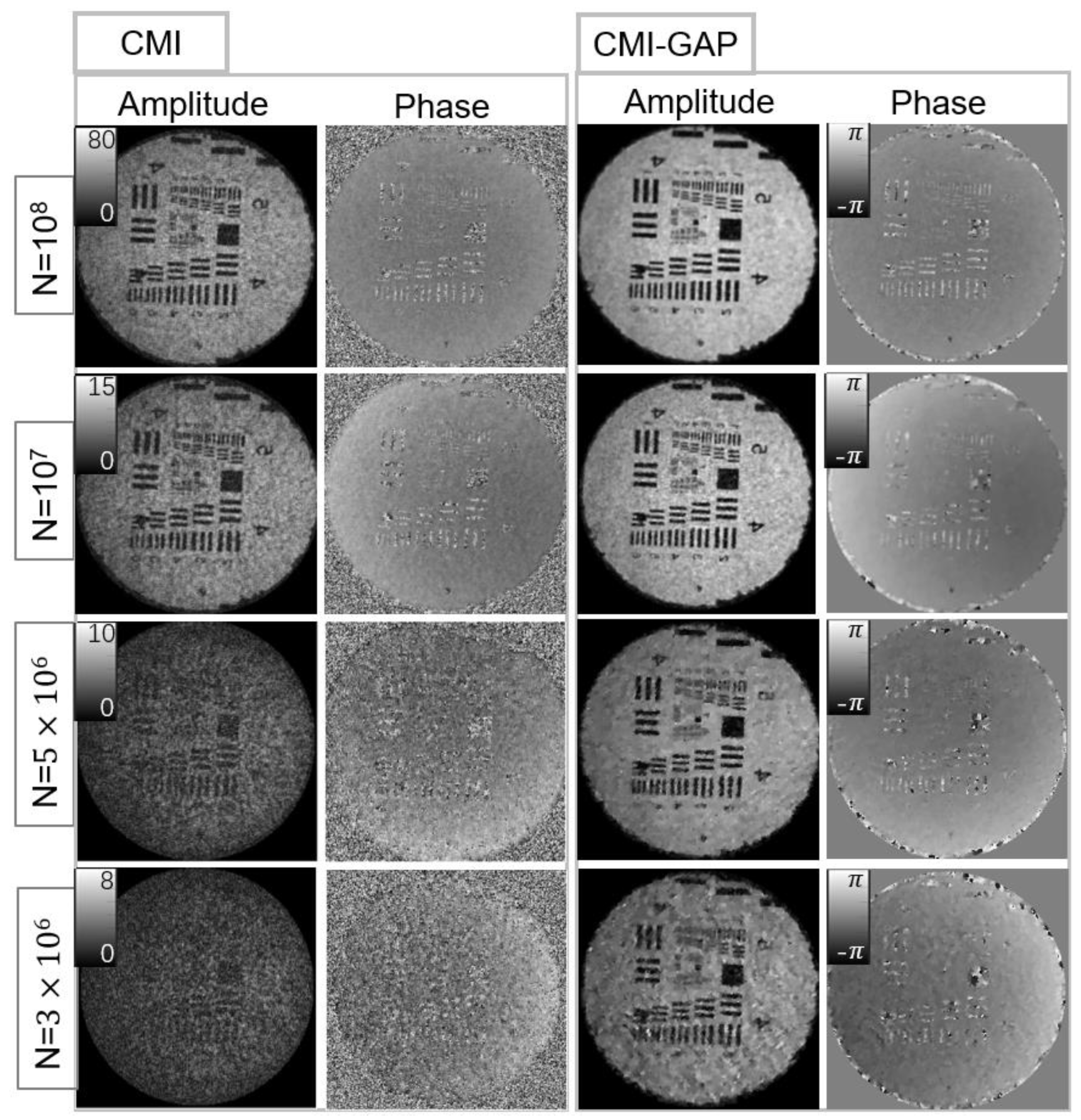
In the near-field experiment, the distance between the sample and the modulator, and the distance between the modulator and the detector, were and respectively. CMI data with four levels of photon flux were acquired. The reconstruction results are shown in Figure 8. The iteration number of the traditional algorithm is about 500 and 50 with CMI-GAP. The overall degradation of quality is believed to be caused by residual reflections and detector noise. From Figure 8, one can see that the amplitude and phase images can be accurately reconstructed when equals to or . In contrast, the reconstruction from the CMI-GAP algorithm has fewer artifacts and a higher resolution. The quantitative comparison, in terms of RMS, is given in Table 1. The ground truth images were obtained by ptychography.
When drops to the traditional CMI algorithm fails to produce a recognizable image, while the proposed algorithm can still reconstruct most of the sample information. Both algorithms failed when the average photon count per pixel dropped to 13.
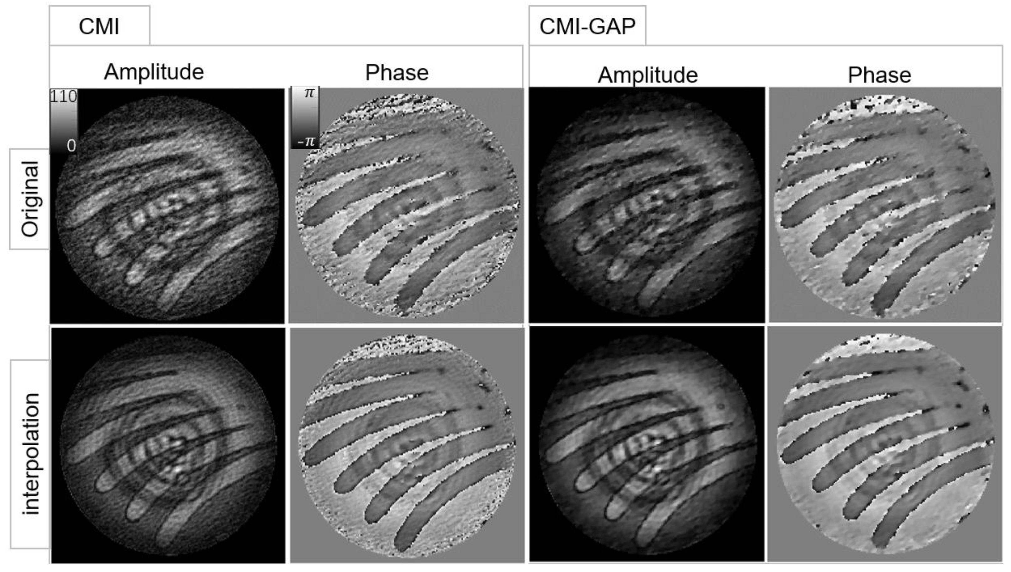
For far-field geometry, we performed optical experiments using setup parameters the same as the simulations. A similar improvement as the near-field scenario was obtained. Here we show the results when applied to the far-field X-ray experiment data [39]. In these experiments, a X-ray was used to form a coherent beam. The illumination probe, carrying about photons, was formed by a pinhole. The modulator was placed at downstream of the object, while the distance between the modulator and the detector with a pixel size was about .
The photon flux was about for this X-ray dataset. The reconstruction results obtained by CMI and CMI-GAP are shown in Figure 9. With the original CMI, the amplitude recovered is drowned by noise. In contrast, reconstructions with fewer artifacts and higher contrast can be seen clearly using the proposed CMI-GAP algorithm. For the X-ray experiment, the detector had a 172 mm pixel, leading to the insufficient sampling of the diffraction patterns. A detector pixel subdivision was then used to better model the detector sampling process. With a 2 × 2 subdivision, the quality is significantly improved for both CMI and CMI-GAP reconstructions, but the CMI-GAP images have a much clean and smooth appearance.
5. Conclusions
We proposed a reconstruction algorithm for low-photon count coherent modulation imaging. The algorithm uses the total variation constraint under the GAP framework. We compared the newly proposed CMI-GAP algorithm with the current algorithm for CMI using extensive simulations and experiments of various levels of illumination photons. The CMI-GAP algorithm still preserves the fast convergence speed and the high robustness against noise of CMI. Our results show the method outperforms the current CMI algorithm in convergence and image quality when the flux of illumination is lower than . When the number of photons was reduced below , CMI failed completely, while some sample features could still be retrieved with the CMI-GAP algorithm. CMI-GAP is robust to noise, with enhancement as much as 20 dB on PSNR and three times on RMS.
The CMI-GAP method could be further extended. First, the algorithmic parameters can be adaptively adjusted to the photon flux level, for which the Adam optimizer could be adopted. Second, the dataset statistics could be incorporated into the algorithm. Third, the continuity of diffraction patterns may be used as prior. It is necessary to mention that the convergence rate will decrease substantially when the computation array gets larger. The possibility of using the ADMM algorithm to accelerate the convergence is worth investigating.
Author Contributions
Methodology, M.S., T.L. and F.Z.; Resources, G.B. and Y.Q. All authors have read and agreed to the published version of the manuscript.
Funding
Natural National Science Foundation of China (NSFC) (12074167, 11775105); Shenzhen Key Laboratory of Robotics Perception and Intelligence (ZDSYS20200810171800001), Southern University of Science and Technology; Shenzhen Science and Technology Program (Grant No. KQTD20170810110313773). Centers for Mechanical Engineering Research and Education at MIT and SUSTech (MechERE Centers at MIT and SUSTech) (No. 6941806); S&T Program of Hebei (No. SZX2020034).
Institutional Review Board Statement
Not applicable.
Informed Consent Statement
Not applicable.
Data Availability Statement
Data underlying the results presented in this paper are not publicly available at this time but may be obtained from the authors upon reasonable request.
Acknowledgments
F.Z. acknowledges Bo Chen, Graeme Morrison, Joan Vila-Comamala, Manuel Guizar-Sicairos, and Ian Robinson for the acquisition of the X-ray data.
Conflicts of Interest
The authors declare no conflict of interest.
References
- Chapman, H.N.; Nugent, K.A. Coherent Lensless X-ray Imaging. Nat. Photon. 2010, 4, 833–839. [Google Scholar] [CrossRef]
- Miao, J.; Ishikawa, T.; Robinson, I.K.; Murnane, M.M. Beyond Crystallography: Diffractive Imaging Using Coherent X-ray Light Sources. Science 2015, 348, 530–535. [Google Scholar] [CrossRef] [PubMed] [Green Version]
- Fienup, J.R. Phase Retrieval Algorithms: A Comparison. Appl. Opt. 1982, 21, 2758. [Google Scholar] [CrossRef] [Green Version]
- Williams, G.J.; Quiney, H.M.; Dhal, B.B.; Tran, C.Q.; Nugent, K.A.; Peele, A.G.; Paterson, D.; de Jonge, M.D. Fresnel Coherent Diffractive Imaging. Phys. Rev. Lett. 2006, 97, 025506. [Google Scholar] [CrossRef] [PubMed] [Green Version]
- Robinson, I.K.; Vartanyants, I.A.; Williams, G.J.; Pfeifer, M.A.; Pitney, J.A. Reconstruction of the Shapes of Gold Nanocrystals Using Coherent X-ray Diffraction. Phys. Rev. Lett. 2001, 87, 195505. [Google Scholar] [CrossRef] [Green Version]
- Barty, A.; Marchesini, S.; Chapman, H.N.; Cui, C.; Howells, M.R.; Shapiro, D.A.; Minor, A.M.; Spence, J.C.H.; Weierstall, U.; Ilavsky, J.; et al. Three-Dimensional Coherent X-ray Diffraction Imaging of a Ceramic Nanofoam: Determination of Structural Deformation Mechanisms. Phys. Rev. Lett. 2008, 101, 055501. [Google Scholar] [CrossRef] [PubMed] [Green Version]
- Barty, A.; Küpper, J.; Chapman, H.N. Molecular Imaging Using X-ray Free-Electron Lasers. Annu. Rev. Phys. Chem. 2013, 64, 415–435. [Google Scholar] [CrossRef]
- Nellist, P.D.; Rodenburg, J.M. Beyond the Conventional Information Limit: The Relevant Coherence Function. Ultramicroscopy 1994, 54, 61–74. [Google Scholar] [CrossRef]
- Fienup, J.R. Reconstruction of an Object from the Modulus of Its Fourier Transform. Opt. Lett. 1978, 3, 27. [Google Scholar] [CrossRef] [Green Version]
- Elser, V. Phase Retrieval by Iterated Projections. J. Opt. Soc. Am. A 2003, 20, 40. [Google Scholar] [CrossRef]
- Marchesini, S. Invited Article: A Unified Evaluation of Iterative Projection Algorithms for Phase Retrieval. Rev. Sci. Instrum. 2007, 78, 011301. [Google Scholar] [CrossRef] [PubMed] [Green Version]
- Chapman, H.N.; Barty, A.; Marchesini, S.; Noy, A.; Hau-Riege, S.P.; Cui, C.; Howells, M.R.; Rosen, R.; He, H.; Spence, J.C.H.; et al. High-Resolution Ab Initio Three-Dimensional x-ray Diffraction Microscopy. J. Opt. Soc. Am. A 2006, 23, 1179. [Google Scholar] [CrossRef] [PubMed]
- Rodriguez, J.A.; Xu, R.; Chen, C.-C.; Zou, Y.; Miao, J. Oversampling Smoothness: An Effective Algorithm for Phase Retrieval of Noisy Diffraction Intensities. J. Appl. Crystallogr. 2013, 46, 312–318. [Google Scholar] [CrossRef] [PubMed]
- Faulkner, H.M.L.; Rodenburg, J.M. Movable Aperture Lensless Transmission Microscopy: A Novel Phase Retrieval Algorithm. Phys. Rev. Lett. 2004, 93, 023903. [Google Scholar] [CrossRef] [PubMed] [Green Version]
- Maiden, A.M.; Rodenburg, J.M. An Improved Ptychographical Phase Retrieval Algorithm for Diffractive Imaging. Ultramicroscopy 2009, 109, 1256–1262. [Google Scholar] [CrossRef] [PubMed]
- Thibault, P.; Dierolf, M.; Menzel, A.; Bunk, O.; David, C.; Pfeiffer, F. High-Resolution Scanning X-ray Diffraction Microscopy. Science 2008, 321, 379–382. [Google Scholar] [CrossRef]
- Pfeiffer, F. X-Ray Ptychography. Nat. Photon. 2018, 12, 9–17. [Google Scholar] [CrossRef]
- Dierolf, M.; Menzel, A.; Thibault, P.; Schneider, P.; Kewish, C.M.; Wepf, R.; Bunk, O.; Pfeiffer, F. Ptychographic X-ray Computed Tomography at the Nanoscale. Nature 2010, 467, 436–439. [Google Scholar] [CrossRef]
- Giewekemeyer, K.; Thibault, P.; Kalbfleisch, S.; Beerlink, A.; Kewish, C.M.; Dierolf, M.; Pfeiffer, F.; Salditt, T.; Robinson, I.K. Quantitative Biological Imaging by Ptychographic X-Ray Diffraction Microscopy. Proc. Natl. Acad. Sci. USA 2010, 107, 529–534. [Google Scholar] [CrossRef] [Green Version]
- Zheng, G.; Horstmeyer, R.; Yang, C. Wide-Field, High-Resolution Fourier Ptychographic Microscopy. Nat. Photon. 2013, 7, 739–745. [Google Scholar] [CrossRef] [Green Version]
- Hruszkewycz, S.O.; Allain, M.; Holt, M.V.; Murray, C.E.; Holt, J.R.; Fuoss, P.H.; Chamard, V. High-Resolution Three-Dimensional Structural Microscopy by Single-Angle Bragg Ptychography. Nat. Mater. 2017, 16, 244–251. [Google Scholar] [CrossRef] [PubMed] [Green Version]
- Holler, M.; Guizar-Sicairos, M.; Tsai, E.H.R.; Dinapoli, R.; Müller, E.; Bunk, O.; Raabe, J.; Aeppli, G. High-Resolution Non-Destructive Three-Dimensional Imaging of Integrated Circuits. Nature 2017, 543, 402–406. [Google Scholar] [CrossRef] [PubMed]
- Holler, M.; Odstrcil, M.; Guizar-Sicairos, M.; Lebugle, M.; Müller, E.; Finizio, S.; Tinti, G.; David, C.; Zusman, J.; Unglaub, W.; et al. Three-Dimensional Imaging of Integrated Circuits with Macro- to Nanoscale Zoom. Nat. Electron. 2019, 2, 464–470. [Google Scholar] [CrossRef]
- Jiang, Y.; Chen, Z.; Han, Y.; Deb, P.; Gao, H.; Xie, S.; Purohit, P.; Tate, M.W.; Park, J.; Gruner, S.M.; et al. Electron Ptychography of 2D Materials to Deep Sub-Ångström Resolution. Nature 2018, 559, 343–349. [Google Scholar] [CrossRef] [PubMed]
- Wang, P.; Zhang, F.; Gao, S.; Zhang, M.; Kirkland, A.I. Electron Ptychographic Diffractive Imaging of Boron Atoms in LaB6 Crystals. Sci. Rep. 2017, 7, 2857. [Google Scholar] [CrossRef] [Green Version]
- Yang, H.; MacLaren, I.; Jones, L.; Martinez, G.T.; Simson, M.; Huth, M.; Ryll, H.; Soltau, H.; Sagawa, R.; Kondo, Y.; et al. Electron Ptychographic Phase Imaging of Light Elements in Crystalline Materials Using Wigner Distribution Deconvolution. Ultramicroscopy 2017, 180, 173–179. [Google Scholar] [CrossRef] [PubMed]
- Yang, H.; Rutte, R.N.; Jones, L.; Simson, M.; Sagawa, R.; Ryll, H.; Huth, M.; Pennycook, T.J.; Green, M.L.H.; Soltau, H.; et al. Simultaneous Atomic-Resolution Electron Ptychography and Z-Contrast Imaging of Light and Heavy Elements in Complex Nanostructures. Nat. Commun. 2016, 7, 12532. [Google Scholar] [CrossRef] [Green Version]
- Thibault, P.; Guizar-Sicairos, M. Maximum-Likelihood Refinement for Coherent Diffractive Imaging. New J. Phys. 2012, 14, 063004. [Google Scholar] [CrossRef]
- Godard, P.; Allain, M.; Chamard, V.; Rodenburg, J. Noise Models for Low Counting Rate Coherent Diffraction Imaging. Opt. Express 2012, 20, 25914. [Google Scholar] [CrossRef]
- Zhou, L.; Song, J.; Kim, J.S.; Pei, X.; Huang, C.; Boyce, M.; Mendonça, L.; Clare, D.; Siebert, A.; Allen, C.S.; et al. Low-Dose Phase Retrieval of Biological Specimens Using Cryo-Electron Ptychography. Nat. Commun. 2020, 11, 2773. [Google Scholar] [CrossRef]
- Huisken, J.; Swoger, J.; Bene, F.D.; Wittbrodt, J.; Stelzer, E.H.K. Optical Sectioning Deep inside Live Embryos by Selective Plane Illumination Microscopy. Sci. New Ser. 2004, 305, 1007–1009. [Google Scholar] [CrossRef] [PubMed] [Green Version]
- Henderson, R. The Potential and Limitations of Neutrons, Electrons and X-rays for Atomic Resolution Microscopy of Unstained Biological Molecules. Quart. Rev. Biophys. 1995, 28, 171–193. [Google Scholar] [CrossRef] [PubMed] [Green Version]
- Laissue, P.P.; Alghamdi, R.A.; Tomancak, P.; Reynaud, E.G.; Shroff, H. Assessing Phototoxicity in Live Fluorescence Imaging. Nat. Methods 2017, 14, 657–661. [Google Scholar] [CrossRef] [PubMed] [Green Version]
- Song, J.; Allen, C.S.; Gao, S.; Huang, C.; Sawada, H.; Pan, X.; Warner, J.; Wang, P.; Kirkland, A.I. Atomic Resolution Defocused Electron Ptychography at Low Dose with a Fast, Direct Electron Detector. Sci. Rep. 2019, 9, 3919. [Google Scholar] [CrossRef] [PubMed] [Green Version]
- Chen, Z.; Odstrcil, M.; Jiang, Y.; Han, Y.; Chiu, M.-H.; Li, L.-J.; Muller, D.A. Mixed-State Electron Ptychography Enables Sub-Angstrom Resolution Imaging with Picometer Precision at Low Dose. Nat. Commun. 2020, 11, 2994. [Google Scholar] [CrossRef]
- Lozano, J.G.; Martinez, G.T.; Jin, L.; Nellist, P.D.; Bruce, P.G. Low-Dose Aberration-Free Imaging of Li-Rich Cathode Materials at Various States of Charge Using Electron Ptychography. Nano Lett. 2018, 18, 6850–6855. [Google Scholar] [CrossRef] [Green Version]
- Hoppe, W. Towards Three-Dimensional? Electron Microscopy? At Atomic Resolution. Naturwissenschaften 1974, 61, 239–249. [Google Scholar] [CrossRef]
- Zhang, F.; Rodenburg, J.M. Phase Retrieval Based on Wave-Front Relay and Modulation. Phys. Rev. B 2010, 82, 121104. [Google Scholar] [CrossRef]
- Zhang, F.; Chen, B.; Morrison, G.R.; Vila-Comamala, J.; Guizar-Sicairos, M.; Robinson, I.K. Phase Retrieval by Coherent Modulation Imaging. Nat. Commun. 2016, 7, 13367. [Google Scholar] [CrossRef]
- Goy, A.; Arthur, K.; Li, S.; Barbastathis, G. Low Photon Count Phase Retrieval Using Deep Learning. Phys. Rev. Lett. 2018, 121, 243902. [Google Scholar] [CrossRef]
- Kang, I.; Zhang, F.; Barbastathis, G. Phase Extraction Neural Network (PhENN) with Coherent Modulation Imaging (CMI) for Phase Retrieval at Low Photon Counts. Opt. Express 2020, 28, 21578. [Google Scholar] [CrossRef] [PubMed]
- Wang, F.; Bian, Y.; Wang, H.; Lyu, M.; Pedrini, G.; Osten, W.; Barbastathis, G.; Situ, G. Phase Imaging with an Untrained Neural Network. Light Sci. Appl. 2020, 9, 77. [Google Scholar] [CrossRef] [PubMed]
- Bandeira, A.S.; Cahill, J.; Mixon, D.G.; Nelson, A.A. Saving Phase: Injectivity and Stability for Phase Retrieval. Appl. Comput. Harmon. Anal. 2014, 37, 106–125. [Google Scholar] [CrossRef]
- Rumelhart, D.E.; Hintont, G.E.; Williams, R.J. Learning Representations by Back-Propagating Errors. Nature 1986, 323, 533–536. [Google Scholar] [CrossRef]
- Zhan, Z.; Cai, J.-F.; Guo, D.; Liu, Y.; Chen, Z.; Qu, X. Fast Multiclass Dictionaries Learning With Geometrical Directions in MRI Reconstruction. IEEE Trans. Biomed. Eng. 2016, 63, 1850–1861. [Google Scholar] [CrossRef] [PubMed] [Green Version]
- Figueiredo, M.A.T.; Nowak, R.D.; Wright, S.J. Gradient Projection for Sparse Reconstruction: Application to Compressed Sensing and Other Inverse Problems. IEEE J. Sel. Top. Signal Process. 2007, 1, 586–597. [Google Scholar] [CrossRef] [Green Version]
- Szlam, A.; Gregor, K.; LeCun, Y. Fast Approximations to Structured Sparse Coding and Applications to Object Classification. In Computer Vision–ECCV 2012; Fitzgibbon, A., Lazebnik, S., Perona, P., Sato, Y., Schmid, C., Eds.; Lecture Notes in Computer Science; Springer: Berlin/Heidelberg, Germany, 2012; Volume 7576, pp. 200–213. ISBN 978-3-642-33714-7. [Google Scholar]
- Gerchberg, R.W.; Saxton, W.O. A Practical Algorithm for the Determination of Phase from Image and Diffraction Plane Pictures. Optik 1972, 35, 6. [Google Scholar]
- Chan, S.H.; Wang, X.; Elgendy, O.A. Plug-and-Play ADMM for Image Restoration: Fixed Point Convergence and Applications. arXiv 2016, arXiv:1605.01710. [Google Scholar] [CrossRef] [Green Version]
- Bioucas-Dias, J.M.; Figueiredo, M.A.T. A New TwIST: Two-Step Iterative Shrinkage/Thresholding Algorithms for Image Restoration. IEEE Trans. Image Process. 2007, 16, 2992–3004. [Google Scholar] [CrossRef] [Green Version]
- Yuan, X.; Liu, Y.; Suo, J.; Dai, Q. Plug-and-Play Algorithms for Large-Scale Snapshot Compressive Imaging. In Proceedings of the 2020 IEEE/CVF Conference on Computer Vision and Pattern Recognition (CVPR), Seattle, WA, USA, 13–19 June 2020; IEEE: Seattle, WA, USA, 2020; pp. 1444–1454. [Google Scholar]
- Chang, X.; Bian, L.; Zhang, J. Large-Scale Phase Retrieval. eLight 2021, 1, 4. [Google Scholar] [CrossRef]
- Gao, Y.; Cao, L. A Complex Constrained Total Variation Image Denoising Algorithm with Application to Phase Retrieval. arXiv 2021, arXiv:2109.05496. [Google Scholar]
- Fienup, J.R. Invariant Error Metrics for Image Reconstruction. Appl. Opt. 1997, 36, 8352. [Google Scholar] [CrossRef] [PubMed]
Figure 1.
The flowchart of the proposed CMI-GAP algorithm. It consists of two parts, forward propagation via CMI and inverse propagation via GAP. The introduction of TV regularization helps improve the performance under low lighting conditions.
Figure 1.
The flowchart of the proposed CMI-GAP algorithm. It consists of two parts, forward propagation via CMI and inverse propagation via GAP. The introduction of TV regularization helps improve the performance under low lighting conditions.

Figure 2.
Reconstruction of the sample given near-field CMI simulated data at varying photon flux. In the lower right corner of each image is a larger version of the middle region. As decreases, the superiority of CMI-GAP is demonstrated clearly.
Figure 2.
Reconstruction of the sample given near-field CMI simulated data at varying photon flux. In the lower right corner of each image is a larger version of the middle region. As decreases, the superiority of CMI-GAP is demonstrated clearly.

Figure 3.
Error metrics comparison of reconstruction in our simulation for a near-field dataset when . Bar charts: PSNR comparison of reconstructed amplitudes under two algorithms. Line graphs: RMS comparison of reconstructed amplitudes under two algorithms.
Figure 3.
Error metrics comparison of reconstruction in our simulation for a near-field dataset when . Bar charts: PSNR comparison of reconstructed amplitudes under two algorithms. Line graphs: RMS comparison of reconstructed amplitudes under two algorithms.

Figure 4.
Convergence curve of the two algorithms in near-field geometry under 3 levels of photon flux. The RMS using our proposed algorithm converges relatively fast and reaches a lower RMS value.
Figure 4.
Convergence curve of the two algorithms in near-field geometry under 3 levels of photon flux. The RMS using our proposed algorithm converges relatively fast and reaches a lower RMS value.

Figure 5.
Reconstruction of the sample given far-field CMI simulated data at varying photon flux. In the lower right corner of each image is a larger version of the middle region. CMI-GAP produces significant enhancement on reconstruction quality.
Figure 5.
Reconstruction of the sample given far-field CMI simulated data at varying photon flux. In the lower right corner of each image is a larger version of the middle region. CMI-GAP produces significant enhancement on reconstruction quality.

Figure 6.
Error metrics comparison of reconstruction in our simulation for the far-field dataset when . Bar charts: PSNR comparison of reconstructed amplitudes under two algorithms. Line graphs: RMS comparison of reconstructed amplitudes under two algorithms.
Figure 6.
Error metrics comparison of reconstruction in our simulation for the far-field dataset when . Bar charts: PSNR comparison of reconstructed amplitudes under two algorithms. Line graphs: RMS comparison of reconstructed amplitudes under two algorithms.

Figure 7.
Convergence curve of RMS for the two algorithms in far-field geometry under 3 levels of photon flux. The CMI-GAP algorithm has a relatively low RMS value and a faster convergence.
Figure 7.
Convergence curve of RMS for the two algorithms in far-field geometry under 3 levels of photon flux. The CMI-GAP algorithm has a relatively low RMS value and a faster convergence.

Figure 8.
Reconstruction of the USAF given near-field CMI experimental data at varying illumination photons. The reconstruction from the CMI-GAP algorithm has fewer artifacts and a higher resolution.
Figure 8.
Reconstruction of the USAF given near-field CMI experimental data at varying illumination photons. The reconstruction from the CMI-GAP algorithm has fewer artifacts and a higher resolution.

Figure 9.
Reconstruction of the far-field CMI experimental data. Top-left: Reconstructed amplitude and phase with original algorithm. Top-right: Reconstructions with proposed algorithm. Bottom-left: Reconstructions of original algorithm with 2 × 2 subdivision. Bottom-right: Reconstructions of proposed algorithm with 2 × 2 subdivision.


Table 1.
RMS corresponding to the near-field CMI.
| Number of Photons | ||||
|---|---|---|---|---|
| RMS of CMI-GAP | 0.17 | 0.31 | 0.45 | 0.62 |
| RMS of CMI | 0.32 | 0.50 | 0.76 | 0.85 |
Publisher’s Note: MDPI stays neutral with regard to jurisdictional claims in published maps and institutional affiliations. |
© 2022 by the authors. Licensee MDPI, Basel, Switzerland. This article is an open access article distributed under the terms and conditions of the Creative Commons Attribution (CC BY) license (https://creativecommons.org/licenses/by/4.0/).
Share and Cite
MDPI and ACS Style
Sun, M.; Liu, T.; Barbastathis, G.; Qi, Y.; Zhang, F. Low-Photon Counts Coherent Modulation Imaging via Generalized Alternating Projection Algorithm. Appl. Sci. 2022, 12, 11436. https://0-doi-org.brum.beds.ac.uk/10.3390/app122211436
AMA Style
Sun M, Liu T, Barbastathis G, Qi Y, Zhang F. Low-Photon Counts Coherent Modulation Imaging via Generalized Alternating Projection Algorithm. Applied Sciences. 2022; 12(22):11436. https://0-doi-org.brum.beds.ac.uk/10.3390/app122211436
Chicago/Turabian StyleSun, Meng, Tao Liu, George Barbastathis, Yincheng Qi, and Fucai Zhang. 2022. "Low-Photon Counts Coherent Modulation Imaging via Generalized Alternating Projection Algorithm" Applied Sciences 12, no. 22: 11436. https://0-doi-org.brum.beds.ac.uk/10.3390/app122211436
Note that from the first issue of 2016, this journal uses article numbers instead of page numbers. See further details here.