
Binary Ebola Optimization Search Algorithm for Feature Selection and Classification Problems

1
School of Mathematics, Statistics, and Computer Science, University of KwaZulu-Natal, King Edward Avenue, Pietermaritzburg Campus, Pietermaritzburg 3201, KZN, South Africa
2
Department of Computer Science, Ahmadu Bello University, Zaria 810211, Nigeria
*
Author to whom correspondence should be addressed.
Appl. Sci. 2022, 12(22), 11787; https://0-doi-org.brum.beds.ac.uk/10.3390/app122211787
Submission received: 20 October 2022
/
Revised: 9 November 2022
/
Accepted: 17 November 2022
/
Published: 19 November 2022
(This article belongs to the Special Issue Evolutionary Algorithms and Large-Scale Real-World Applications)
Abstract
:In the past decade, the extraction of valuable information from online biomedical datasets has exponentially increased due to the evolution of data processing devices and the utilization of machine learning capabilities to find useful information in these datasets. However, these datasets present a variety of features, dimensionalities, shapes, noise, and heterogeneity. As a result, deriving relevant information remains a problem, since multiple features bottleneck the classification process. Despite their adaptability, current state-of-the-art classifiers have failed to address the problem, giving rise to the exploration of binary optimization algorithms. This study proposes a novel approach to binarizing the Ebola optimization search algorithm. The binary Ebola search optimization algorithm (BEOSA) uses two newly formulated S-shape and V-shape transfer functions to investigate mutations of the infected population in the exploitation and exploration phases, respectively. A model is designed to show a representation of the binary search space and the mapping of the algorithm from the continuous space to the discrete space. Mathematical models are formulated to demonstrate the fitness and cost functions used for evaluating the algorithm. Using 22 benchmark datasets consisting of low, medium and high dimensional data, we exhaustively experimented with the proposed BEOSA method and six other recent similar feature selection methods. The experimental results show that the BEOSA and its variant BIEOSA were highly competitive with different state-of-the-art binary optimization algorithms. A comparative analysis of the classification accuracy obtained for eight binary optimizers showed that BEOSA performed competitively compared to other methods on nine datasets. Evaluation reports on all methods revealed that BEOSA was the top performer, obtaining the best values on eight datasets and eight fitness and cost functions. Computation for the average number of features selected showed that BEOSA outperformed other methods on 11 datasets when population sizes of 75 and 100 were used. Findings from the study revealed that BEOSA is effective in handling the challenge of feature selection in high-dimensional datasets.
1. Introduction
Machine learning and data mining are fast-growing topics in research and industry because of the massive amount of data being generated which needs to be converted into usable information. This conversion process plays an essential part in the process of knowledge discovery, as it comprises a set of repetitive task sequences including the transformation, reduction, cleansing, and integration of data, among others [1]. These steps are known as pre-processing; their outcome directly impacts the machine learning and data mining algorithm performance. Due to its importance, data is regarded as the “currency” of the present decade. This makes the correct handling of data a necessity. With the increase in data and the growth of machine learning and data mining, the processing of data is becoming more and more tedious. The increase in dimensionality means that training machine learning and data mining algorithms takes longer, making them more computationally expensive. Researchers have developed different methods to address the problem of dimensionality. One such method is feature selection, which removes the presence of noisy data such as unnecessary or useless features that do not assist with the purpose of classification [2].
Feature selection is a pre-processing stage which assists in selecting valuable features and separating them from a set of unwanted ones, thereby improving the performance of the classifiers. This method eradicates redundant, irrelevant features, thereby reducing time complexity [3]. Feature selection is generally performed in two ways, namely, wrapper and filter methods [4]. The wrapper method utilizes learning algorithm(s) to choose the subsets of features. This method produces better performance but is more computationally expensive than the filter method. The feature selection under the wrapper technique is referred to as an optimization problem [5]. The filter-based technique does not depend on a learning algorithm; rather, it chooses useful features by utilizing information gain, mutual information etc. [6]. This method is computationally inexpensive but does not produce as good a performance as the wrapper-based techniques. Finding the relevant subset of features is a challenging task, as the main aim is to select the minimum number of features and get the maximum accuracy possible. Due to the increased time required to locate the optimal subset of features, feature selection is referred to as an NP-hard problem [7]. Should we have an feature, the sum of of the number of the combination of features is needed to investigate and locate the best features [8]. The need for a high-performing metaheuristic to take care of this type of problem is important to reduce the processing time. The search processes of metaheuristics rely on the trade-off between the exploitation (intensification)—that conducts a thorough neighborhood search to obtain better possible solutions—and exploration (diversification)—that tests the solution of candidates not within the neighborhood. These two objectives are the factors that define the ability to find optimal solution(s). Recently, feature selection as an optimization problem has been solved using metaheuristic algorithms because they show better performance than exact methods [8,9,10,11,12,13]. However, due to the no free lunch (NFL) theorem, which proposes that no one algorithm is sufficient to solve all optimization problems, the need to develop new or improve existing methods that can make high-quality solutions for the candidate problem becomes unavoidable.
Despite the great effort and advancements in this area, most metaheuristic algorithms have at least one deficiency or shortcoming. Examples of such limitations include getting trapped in local optima, premature convergence, too many parameters to be tuned and so on. The question which raises serious research opportunity is: does good performance and the superiority demonstrated by a continuous variant of an optimization algorithm translate into similar good performance when applied to solve binary optimization problems? To answer this question, this paper presents a binary Ebola optimization search algorithm (BEOSA) to solve the feature selection problem and to avoid some of these drawbacks. The baseline EOSA is a recently proposed metaheuristic algorithm [14], a bio-based algorithm inspired by the Ebola virus disease propagation model. The base algorithm was evaluated on 47 classical benchmark functions and compared with seven well-known techniques and 14 CEC benchmark functions, producing superior performance over other methods in the study. This consideration and the selection of the EOSA method as the base algorithm for the binary optimization method proposed in this study was motivated by the performance of the algorithm itself and even a recent outstanding report of its immunity-based variant, namely, IEOSA. The performance of this biology-based algorithm stood out among most of the state-of-the-art optimization methods with similar sources of inspiration. Since the algorithm has proven relevant in addressing some very difficult continuous optimization problems, we sought to determine whether its operators and optimization process could find optimal solutions for binary optimization problems. Hence, through an exhaustive and rigorous experimentation on several heterogeneous and high-dimensional datasets, this study investigates the influence, impact and benefit of designing and applying a binary variant of the EOSA/IEOSA methods. The performance of this method was the motivation for this binarization, and since this method was developed, it has not been utilized to solve the feature selection problem. Since the feature selection problem is binary, we present a binary version of the EOSA to solve this problem. We also utilize the k-near neighbor (kNN) as the classifier to test the goodness of the selected subset of features. The the major contributions of this work are as follows:
- Proposal of the binary version of the EOSA algorithm (called BEOSA) for feature selection problems.
- Evaluation of the performance of BEOSA using a convergence curve and other computational analysis metrics.
- Evaluation and validation of the proposed method with 22 small and medium size and 3 high-dimensional datasets.
- The proposed method was assessed using seven classifiers to evaluate its performance.
- A comparison is made of the efficacy of the BEOSA with some other popular feature selection methods.
The remainder of this manuscript is structured as follows: Section 2 presents a review of the relevant literature. Section 3 discusses the methodology used in this study. Section 4 details our proposed BEOSA approach and its application in feature selection. Section 5 centers on the results of the experiments and presents a discussion of this work. Section 6 provides the conclusion.
2. Related Work
A detailed review of related studies on the subject of the concept described in this study is presented in this section. The literature shows that several binary metaheuristic algorithms have been developed to solve the feature selection problem. The feature selection technique based on the wrapper approach uses the binary search capability of metaheuristic algorithms. Swarm- and evolutionary-based algorithms are becoming commonplace methods in the feature selection domain [15].
Particle Swarm Optimization (PSO) [16] is a bio-inspired metaheuristic method which has attracted much attention due to its tested and trusted mathematical modelling. This algorithm has been binarized and enhanced to solve problems in discrete search spaces. A study by Unler and Murat [17], presented a modified discrete PSO that used the logistic regression model and applied it to the feature selection domain. A year later, Chuang et al. [18], proposed an improved BPSO that introduced the effect of catfish, called “catfishBPSO”, for feature selection. The BPSO was also improved to tackle the optimization problem of feature selection [19]. Ji et al. [13], proposed an improved PSO based on the Levy flight local factor, a weighting inertia coefficient based on the global factor and a factor of improvement based on the mechanism of mutation diversity, called (IPSO), to tackle the feature selection problem. This improvement came with shortcomings, however, such as the inclusion of more parameters compared with other improved versions of the PSO, which makes tuning difficult for various application problems and increases computational time. Since every particle in BPSO moves closer to and farther from the hypercube corner, its major shortcoming is stagnation.
The genetic algorithm (GA) is another popular bio-inspired feature selection method which has been widely utilized as a wrapper-based technique. Huang and Wang [20], proposed a GA-based method using the support vector machine (SVM) as a learning algorithm to solve the feature selection problem. The major goal of their work was concurrent parameter and feature subset optimization without reducing the classification accuracy of the SVM. The method reduced the number of feature subsets and improved the accuracy of classification but was outperformed by the Grid algorithm. Later, Nemati et al. [21], presented a hybrid GA and ant colony optimizer (ACO) as a feature selection method to predict protein functions. These two algorithms were combined to enable better and faster capabilities with very low computational complexity. Furthermore, Jiang et al. [22], proposed a modified GA (MGA), i.e., a feature selection method using a pre-trained deep neural network (DNN) for the prediction of the demand for different patients’ key resources in an outpatient department.
Apart from these two notable algorithms, several other nature-inspired methods have been utilized to solve feature selection problems. The binary wrapper-based bat algorithm was developed by Nakamura et al. in 2012 [23]. It uses the classifier optimum-path forest to locate the feature sets that produce maximum classification accuracy. Hancer et al. [24], proposed a binary artificial bee colony (ABC) that employed a similarity search mechanism inspired by evolution to resolve the feature selection problem. Emary et al. [11], proposed the binary ant lion optimizer (BALO) which utilizes the transfer function as a means of moving ant lions within a discrete search space. The binary grey wolf optimizer with two techniques was proposed the following year to locate a subset of features that cater for the two conflicting objectives of the feature selection problem, i.e., to maximize the accuracy of the classification and minimize the number of selected features. However, this method was plagued with premature convergence, despite its outperformance of other methods used for comparison in the study. Zhang et al. [25], designed a variation of the binary firefly algorithm called return-cost-based FFA (Rc-FFA), which was able to prevent premature convergence. A binary dragonfly optimizer was developed by Mafarja et al. [26], which employed a time-varying transfer function that improved its exploitation and exploration phases. However, its performance was not close to optimal.
Faris et al. [27], proposed two variants of the salp swarm algorithm (SSA) to solve the feature selection problem. The first utilized eight transfer functions to convert a continuous search space to a binary one, and the other introduced a crossover operator to improve the exploration behavior of the SSA; however, the study did not provide an analysis of the transfer functions. A binary grasshopper optimization algorithm (BGOA) was proposed by Mafarja et al. [28], using the V-shaped transfer function and sigmoid. This study incorporated the mutation operator to enhance the exploration phase of the BGOA. In Mafarja and Mirjalili [29], two binary versions of the whale optimization algorithm were proposed. The first utilized the effect of a roulette wheel and tournament mechanisms of selection with a random operator in the process of searching, while the second version employed the mutation and crossover mechanisms to enhance diversification. Kumar et al. [30], proposed a binary seagull optimizer which employed four S- and V-shaped transfer functions to binarize the baseline algorithm, applying it to solve the feature selection problem. The reported results showed competitive performance with other methods; their technique was also evaluated using high-dimensional datasets.
Elgin Christo et al. [31], and Murugesan et al. [32], designed bio-inspired metaheuristics comprising three algorithms. The former combined glowworld swarm optimization, lion optimization algorithm and differential evolution, while the latter hybridized krill herd, cat swarm and bacteria foraging optimizers, with both using the AddaBoostSVM classifier as the fitness function and a backpropagation neural network to perform classification, which was applied to clinical diagnoses of diseases. The methods showed superior performance over other methods. However, these proposed methods were computationally expensive due to the use of combinations of different metaheuristic methods. Balasubramanian and Ananthamoorthy [33], proposed a bio-inspired method (salp swarm) with kernel-ELM as a classifier to diagnose glaucoma disease from medical images. The results produced by this method showed superior performance over other methods. However, the technique was not tested on collections of large, real-time datasets because this proved to be more challenging. The different algorithms mentioned above provided better solutions to many of the feature selection problems [34]. Many of these methods, however, could not yield an optimal subset of features for datasets of high-dimensional magnitude. Additionally, the inference from the NFL theorem that no single algorithm can solve all optimization problems holds in the feature selection domain as well. Hence, a new binary method needs to be developed to solve the optimization problem of feature selection.
Some bio-inspired metaheuristic algorithms are based on susceptible infectious recovery (SIR), the class of models to which the EOSA algorithm belongs. Therefore, reviewing some efforts made using this model in the literature is appropriate here. Some such methods have been proposed to tackle the problem of detection and classification, among which we may cite the SIR model [35]. This approach is based on sample paths and was employed to detect the sources of information in a network. The assumption of that study was that all nodes on the network were in their initial state and were susceptible, apart from a source that was in a state of infection. The susceptible nodes could then become infected by the infected node, which itself may have no longer been infected. The result of this simulation revealed that the estimator that the reverse-infection algorithm produced for the tree network was nearer to the real source. A further performance evaluation was conducted on many real-world networks with good outcomes. However, the assumption of a single source node only was the drawback of this model, since, in most real-world scenarios, this is close to impossible. To overcome this problem, Zang et al. [36], utilized a divide-and-conquer approach to find many sources in social networks using the SIR model. The technique showed promising results with high accuracy of its estimations. However, these methods have not been directly employed in the feature selection optimization problem.
Since the outbreak of the COVID-19 virus in 2020, more SIR model-based methods have been designed to detect or diagnose corona virus infection in humans. In Al-Betar et al. [37], a new coronavirus herd immunity optimizer (CHIO) was proposed which drew its inspiration from the concept of herd immunity and social distance strategy so as to protect society from contracting the virus. The herd immunity employed three main kinds of individuals: susceptible, infected and immunized; it was applied to solve engineering optimization problem. This algorithm has since been utilized to solve feature selection and classification problems, including the introduction of a novel COVID-19 diagnostic strategy, known as patient detection strategy (CPDS) [38], that combined the wrapper and filter methods for feature selection. The improved k-near neighbor (EKNN) was used for the wrapper method using the chest CT images of COVID-19 infected and non-infected patients. The results revealed the superiority of the proposed method over other, recently developed ones in terms of accuracy, sensitivity, precision, and time of execution. Similarly, the greedy search operator was incorporated with and without the CHIO to make two wrapper-based methods, which were evaluated on 23 benchmark datasets and a real-world COVID-19 dataset.
Some high-dimensional datasets have been employed to assess the efficacy of the proposed methods. Alweshah [39], boosted the efficiency of the probabilistic neural network (PNN) using CHIO to solve the classification problem. Eleven benchmark datasets were used to assess the accuracy of classification of the proposed CHIO-PNN which, on all the datasets used, produced a summative classification rate of 90.3% with a quicker rate of convergence than other methods. However, the drawback of this method was its use on low and medium rank datasets. As such, there is a concern that higher dimensional datasets may negatively impact its performance.
3. Methodology
This section presents the methodology of the proposed binarization approach for the EOSA algorithm. To achieve the design, an overview of the EOSA algorithm and its immunity-based variant is presented. This is followed by a description of the procedure for the generation and binarization of the search space. The binary variant of EOSA is then formulated and incorporated into the binary search space. The variant can use the proposed transformation functions to map the continuous space to a discrete space. The classification models used to support the feature selection process are also discussed.
3.1. Overview of EOSA and IEOSA
The EOSA metaheuristic [14] was inspired by the classical SIR model and the propagation model of the Ebola virus. Drawing from the natural phenomena associated with the development of immunity by individuals against virus strains and the potential coverage an immune individual provides for a susceptible individual, a new variant was proposed, named immunity-based variant (IEOSA). Both the base algorithm and the immunity-based variant were exhaustively tested using continuous benchmark functions. The obtained results confirmed their viability. We present a summary of the mathematical models of the methods to support discussion of the techniques for the proposed BEOSA and BIEOSA. The population initialization of EOSA and IEOSA is undertaken as shown in Equations (1) and (2).
where is a constant (3), is a randomly generated real number, is the lower bound and is the upper bound of the optimization problem. The mutation of infected individuals in the continuous space is described by Equation (3), where is the change factor of an individual and is a global best solution.
The calculations for the allocation of individuals to compartments I, R, D, H, V and Q were detailed in [14,40]. Considering the increasing demand for solving binary optimization problems and the outstanding performance reported by the EOSA method, the binary EOSA (BEOSA) is proposed in this study. In the following subsections, we include a detailed discussion on the design of the algorithm for BEOSA and BIEOSA.
3.2. Binarization of Search Space
The BEOSA search space consists of individuals whose representations are of the binary search space form. The entire population represents individuals whose anatomies are made up of binary digits. This representation is required to aid in the processes of identification and differentiation of selected features from those which are not. Figure 1 presents an illustration of the entire search space for the BEOSA algorithm. First, the population of individuals in the search space is determined according to two parameters, namely, population size and the dimension of dataset . is obtained by computing the number of features in dataset , while is declared during the initialization of the population. Following an iterative approach, each individual in the population is initialized to a value of 1 for the whole of dimension in . It is expected that the application of the BEOSA operation on the search space will result in optimized solutions whose internal representation will have been modified to values between 0 and 1 for the whole of the dimension in .
The complete optimization process, which is expected to run for a number of iterations, will yield output for each individual , similar to what is shown in Figure 2. It is assumed that cells whose values are 1 s are considered to translate into the features which have been selected. Recall that the dimension of for arbitrary solution is similar to the number of features in the dataset of . As a result, we simply count the number of 1 s in the dimension of for every which represents the instances in the dataset .
The formalization of the search space is necessary to support the process of binarization of EOSA which is suitable for solving the problem of feature selection. In the following subsection, we describe the composition of the proposed BEOSA method.
3.3. Binarization of EOSA (BEOSA)
The design of the new variant of EOSA which will be able to optimize solutions in a discrete solution space applies some new operators to existing ones in the algorithm. The first is the definition of transformation functions which can change the solution representation and optimization process from a continuous form to a discrete one. This is necessary to allow the new method to process problems which are peculiar to feature selection. The second operation modelled to achieve the new variant BEOSA is modifying the fitness function. Evaluating the solutions to find the global best among all individuals requires that the fitness of the solutions be computed. The definition of the fitness function is presented to suit the problem domain. Furthermore, the design of the BEOSA algorithm and a flowchart are presented and discussed.
3.3.1. Transformation of Method
We proposed four transformation functions to position infected individuals in the discrete space. These functions follow the popular S-functions and V-functions categories, so that two functions are described for the latter and two for the former. Equations (4) and (5) contain the S1 and S2 functions which belong to the S-transform function, while Equations (6) and (7) contain the V1 and V2 functions which belong to the V-function family.
In Figure 3, the behavior of the transform functions is plotted to show that they are truly able to generate patterns similar to the class of function they belong to. For instance, the (a) part of the figure shows that the two S-functions result in an S-shaped pattern when the function is applied to values [−6, 6], while a V-shaped pattern is reported for the V-functions when they are applied to the same values. Note that these functions confine their output on the y-axis to values between [0, 1], which is the aim of using the transform functions.
The aim of applying these transform functions is to ensure that they can help transfer the composition of feature positions in an individual to either 0 or 1. Additionally, these functions can increase the probability of changing the natural composition of that individual, so that they become a potential solution for solving feature selection problems. This is illustrated using Equations (8) and (9). The first part of the two equations controls the selection of either the S1 or S2 function when applying the S-function and the use of either T1 or T2 when applying the V-function. A determinant factor is used to guide this decision, so that if , the function generates 1, and the S2 or T2 function is called as appropriate; otherwise, the S1 or T1 function is called. In the second part of the two equations, the value of the position in the representation of individual is modified to be 1 when for S-functions and for T-functions; otherwise, 0 is assigned to the position whereby k lies between , and is a randomly generated between [0, 1].
A flowchart of the process of applying the transform functions to achieve the translation of the BEOSA from the continuous space to the discrete space is illustrated in Figure 4. The optimization process begins with a population described as the susceptible group. Based on the natural phenomenon of the EOSA method, some individuals are exposed to the virus, thereby leading to some of them being allocated to the infected subgroup. It is these infected individuals that are optimized for a number of iterations. It is expected that during the iteration, almost all the members of the susceptible subgroup will move to the infected subgroup. For each in the subgroup, the position is mutated using either of the S-functions or V-functions, depending on the satisfiability of the criteria. Note that the function computes the current position and displacement of individual . A constant value of 0.5 was assumed for the parameter during experimentation. The satisfiability of this condition determines whether the S-functions or the V-function will be applied. The final output of the optimization process is in a vector of 0 s and 1 s, as shown in Figure 4.
The mutation of the values of the position in every in the subgroup and the termination of the iterative condition will lead to the evaluation of the fitness values of each individual in the entire population, thereby determining the current global best solution for solving the feature selection problem. The following subsection discusses the fitness function used in this study.
3.3.2. Fitness and Cost Functions
A combination of both the fitness function evaluation and the cost function evaluation was used to locate the best-performing solution to solve the feature selection problem. The fitness function in Equation (10) evaluates the solution based on its performance on classifier on subset of the dataset and with the application of control parameter . The notation , as used in the equation, returns the number of 1 s in the array representing individual . Note that the notation returns the number of features selected in the individual, while represents the dimension of the features in dataset . For experimental purposes, a value of 0.99 was used for .
In Equation (11), the cost function is evaluated from the output of the fitness function, i.e., by simply subtracting the value returned by from 1. Both the fitness and cost function values are graphically applied to analyze and interpret the relevance and quality of every best solution obtained for each dataset.
In the following subsection, we demonstrate how these functions are used in the description of the proposed BEOSA method.
3.3.3. BEOSA Algorithm and Flowchart
The representative models for the binary search space and mathematical models described in the previous subsections are formalized using the algorithm and flowchart presented in this subsection. First, we present the algorithmic formalization as seen in Algorithm 1, which indicates that the values for (maximum number of iterations), (population size), (short distance rate) and (long displacement rate) are required for input, while the output of the algorithm is the global best solution, the cost values for each iteration and the feature count obtained for the optimization process. The binarization of the solution space and computation of the fitness values for each solution are listed in Lines 4–5. The current global best solution and the displacement positions for all individuals in the susceptible compartment are computed in Lines 6–7. In Lines 8–34, the iteration for the optimization process is described, given the satisfiability of two conditions: the number of maximum iterations is not reached, and some individuals remain infected. An estimation of the number of individuals to quarantine from the infected is computed, and a declaration of the separation of quarantined from infected individuals is made, in Lines 9–10. Iteration of the infected individuals is declared in Line 11, and the number of newly infected cases in the susceptible group is shown in Line 12. In Lines 13–28, we iterate the newly infected cases and generate the discriminant value in Line 14. If the evaluation of the condition in Line 15 is true, then it implies that the method will search within a local space; otherwise, it will search in a global space. In each case of exploitation and exploration, we compute the anticipated number of infections. In Lines 17–21, we apply the or function, depending on the value of . Additionally, depending on the satisfiability of the condition in Line 18, the feature position in that individual is mutated to either 1 or 0. A similar procedure is repeated for the exploration phase using the or function, depending on the value of . Finally, the compartments are updated and the global best solution is determined before executing the next iteration.
| Algorithm 1 Pseudocode of the BEOS Algorithm |
|
Figure 5 is a flowchart of the entire optimization process of the algorithm. The figure provides a representation of the entire algorithm using a graphical method, including a graphic representation of the flow of the use of the transformation functions. The parting points for the S-functions and T-functions are shown clearly. The flowchart shows the initialization of the population and the global best updates upon the completion of an iterative process.
In the following subsection, we describe the various classifiers applied in this study to obtain the fitness and cost values of the BEOSA method.
3.4. Feature Selection and Count
The computation of the fitness and cost functions largely depends on the classification accuracy obtained by using a classifier on a selected fragment of the dataset. In this study, an investigative exploration was carried out to determine the influence of different popular classifiers in solving the feature selection problem. Although the K-nearest-neighbor (KNN) was used as the base classifier, we applied the random forest (RF), multi-layer perceptron (MLP), decision tree (DT), support vector machine (SVM), and Gaussian Naive Bayes (GNB) classifiers as well. On this basis, the number of features selected for arbitrary individual is computed using Equation (12), where and represent the dimension of the feature size in the dataset and the number of feature positions with 1s in individual , respectively.
The following listing summarizes and describes the procedures and parametrization used for each of the classifiers investigated in this study:
- (a)
- KNN model: this model solves the classification problem by obtaining K-sets of items sharing some similarity. k-fold values of 5, 3 and 2 were investigated to ascertain the most viable settings. For most of the applied datasets, we found a k-fold of 5 to yield optimal performance, whereas in the case of the Iris and Lung datasets using the BSFO algorithm, we found a k-fold of 2 to be optimal.
- (b)
- DT model: similar to the KNN, this study found that k-fold values of 5 and 2 were more suitable for most algorithms and the datasets studied. A significant number of the experiments showed impressive performance using a k-fold of 5. Meanwhile, the maximum depth used for the decision tree model was 2.
- (c)
- RF model: the classification task of RF for all of the benchmark datasets that were applied using the proposed algorithm was tested using 300 estimators, while the k-fold used for the cross-validation operation remained at 5.
- (d)
- MLP model: the MLP model was tested with the settings of 0.001 for the alpha parameter and with hidden layer sizes of the tuple (1000, 500, 100). The model was trained over 2000 epochs with a random state of 4. Additionally, a k-fold of 5 was used for the cross-validation task.
- (e)
- SVM model: the SVM undertakes its classification operation by identifying a decision boundary which is approximate enough to separate items in a dataset into classes. The linear function was applied for the kernel settings, while a C value of 1 and a k-fold value of 5 were investigated with the proposed BEOSA and BIEOSA algorithms.
- (f)
- GNB model: The default values for the parameters of the GNB model were applied for the experimentation, although we manually set the k-fold value to 5 for the cross-validation task. These default parameters demonstrated optimal performance in computing the probability value, which may be described as follows: given class label and feature vector , we can compute the probability of when that of is known, as shown in Equation (13).
In the next section, we present a detailed discussion of the experimental settings and computational environment with the datasets used to test the method presented in this section.
4. Experimental Setup
A description of the experimental configuration is presented in this section. We first note that the computational environment used for our experiments was a personal computer (PC) with the following configuration: CPU, Intel® Core i5-4210U CPU 1.70 GHz, 2.40 GHz; RAM of 8 GB; Windows 10 OS. We also experimented on a series of computer systems with the following configuration: Intel® Core i5-4200, CPU 1.70 GHz, 2.40 GHz; RAM of 16 GB; 64-bit Windows 10 OS. The binary metaheuristic algorithms were implemented using Python 3.7.3 and supporting libraries, such as Numpy and other dependent libraries. While this describes the computational environment, the following subsections detail the parameter settings and the nature of the input supplied during the experiments. This section also presents and justifies the selection of some of the evaluation metrics applied for our comparison of results.
4.1. Dataset
Exhaustive experimentation with BEOSA was carried out using 22 benchmark and popularly available datasets [41]. These datasets have been widely used for comparative analyses of binary metaheuristic algorithms and were therefore considered suitable for testing the efficiency and performance of the method proposed in this study. Table 1 provides some information about the applied datasets. High, moderate and low-dimension datasets are included, making them suitable for experimenting with the BEOSA method on those three dimensions. This became necessary, considering the importance of investigating the suitability of an algorithm on a variety of datasets, high-dimension ones in particular, since these often have similarities with real-life binary optimization problems.
The number of biomedical datasets is growing rapidly; this has led to the generation of high-dimensional features that negatively affect the classifiers of machine learning processes [42]. Many of the feature selection methods described in the literature suffer from diversity of population and local optima problems when they are evaluated against high-dimensional datasets, such as the ever-growing body of biomedical datasets. Feature selection is aimed at selecting the most effective features from an original set containing irrelevant elements; this becomes especially challenging to with high-dimensional datasets, which is why it is important for us to prove the efficacy of the BESOA with such data dimensionality.
The Lung, Prostate, Leukemia, KrVsKpEW, Colon and WaveformEW datasets are considered here as high-dimensional datasets with feature sizes ranging between 4 and 7070. Additionally, most of these datasets have binary classification problems or, in the case of Lung and WaveformEW, multi-classification problems. BreastEW, Exactly, Exactly2, M-of-n and Tic-tac-toe are medium-sized dimensional datasets. Most of the datasets in this category have a number of instances between 9 and 203, and numbers of features are mostly more than 270, except for Iris, which has about four features. Meanwhile, are all binary classification problems. Low-dimensional datasets are those considered to have <500 instances and probably fewer features. The CongressEW, Iris, HeartEW, Ionosphere, Lymphography, PenglungEW, Sonar, SpectEW, Vote and Zoo datasets are in this category. The Iris dataset demonstrates exceptional characteristics, since only four features exist in that dataset, but each has 150 instances. All are binary classification problems except for PenglungEW, Zoo and Lymphography, which are multi-classification problems.
A description of each of these datasets is included. Most share some biological features, while the rest were collated from various other domains.
4.2. Parameter Configuration and Settings
Eight binary variants of metaheuristic algorithms were employed for a comparative analysis with the method proposed in this study, i.e., the binary dwarf mongoose optimizer (BDMO) [14], the binary simulated normal distribution optimizer (BSNDO), the binary particle swarm optimizer (BPSO), the binary whale optimization algorithm (BWOA), the binary sailfish optimizer (BSFO), the binary grey wolf optimizer (BGWO), BEOSA and BIEOSA. Table 2 lists the parameter settings applied for each of the algorithms. The values for the parameters π, β1, β2, β3 and β4, as used in our experiments with BEOSA and BIEOSA, are listed in the table as 0.1, 0.1, 0.1, 0.1 and 0.1, respectively. Similarly, the values for nb, na, ns, peep, and L were set at 3, (N-nb), (n-nb), 1, [0,1] and round (0.6*D*nb) for BDMO. The mean of the population size was computed to set the mo parameter of the BSNDO. Additionally, the BPSO control parameters c1, c2, W and Vmax were initialized at 2, 2, 0.9 and 6. The parameters for the remaining algorithms are shown in the table, with p, l, b r, and C for BWOA being initialized at [0,1], [0,1], 1, [0,1] and 2r. In BSFO, p was 0.1, A was 4 and epsilon was 0.001. Lastly, BGWO was initialized within the bound [2, 0] as coefficient for decreasing power attack.
Population sizes of 25, 50, 75 and 100 were investigated for each of the algorithms to show how this variable affected performance. The training of the algorithms followed 50 iterative processes, and the experiment for each algorithm was typically repeated 10 times/runs to determine the average performance. The formulae applied to compute these averages and all other similar metrics used for our comparative analysis are presented in the following subsection.
4.3. Evaluation Metrics
The evaluation metrics presented in the following paragraphs describe the approach used to quantify the obtained values to support our performance comparison. The following metrics are discussed: classification accuracy, mean accuracy, best accuracy and the standard deviation fitness obtained using Equations (14)–(16).
- (a)
- Classification accuracy (CA): this computes the accuracy of classifier with dataset and label , as described in Equation (14):
- (b)
- Mean accuracy (MA): this computes the mean of all classification accuracies obtained after a certain number of runs on a given algorithm, where is the accuracy obtained during iteration after iterations and all accuracy values obtained for times, as described in Equation (15):
- (c)
- Best Accuracy (BA): the best of all classification accuracies obtained after a certain number of runs, as described in Equation (16):
- (d)
- Average feature count (AFC): obtained by finding the average value for all numbers of selected features for all population groups , as described in Equation (17):
The following section presents the results of all experiments and a comparative analysis of the algorithms. Additionally, the findings derived from the results are highlighted.
5. Results and Discussion of Findings
The results presented in this section are focused on the performance of BEOSA and BIEOSA in comparison with those of similar methods, i.e., the binary dwarf mongoose optimizer (BDMO) [3], the binary simulated normal distribution optimizer (BSNDO) [9], the binary particle swarm optimizer (BPSO) [53], the binary whale optimization algorithm (BWOA) [54], the binary grey wolf optimizer (BGWO) [55] and the binary sailfish optimizer (BSFO) [56] algorithms. The selection of these algorithms was based on their outstanding performance, as described in various reports, and their status as state-of-the-art methods for binary optimization. We note that our evaluations of most of these algorithms applied the same parameterizations, e.g., the number of iterations and parameter settings. The following subsections are organized as follows. Firstly, we provide a comparative analysis of the various methods based on their fitness performance and the number of selected features. We then examine the classification accuracy of each method as compared with others. Next, we compare the cost functions of all methods and show the impact of the choice of classifiers on the feature classification procedure. Finally, we report the computational time of each method and discuss our findings. The following subsections using tabular and graphical means for the sake of clarity.
5.1. Comparative Analysis of Fitness and Cost Functions
BEOSA and BIEOSA are now compared with related algorithms based on the results obtained for fitness and cost functions. The fitness function aims to minimize the objective function, while the cost function aims to maximize it. Table 3 lists the results obtained for each of the binarized algorithms for all benchmark datasets.
The BWOA algorithms performed better on the BreastEW, Lung, Iris, Exactly2, Colon and Vote datasets, with fitness values of 0.0307, 0.0006, 0.0050, 0.2384, 0.0004 and 0.0013, respectively. BWOA showed superiority with six benchmark datasets, while BGWO showed superiority with WaveformEW, yielding a fitness value of 0.1817. BSNDO outperformed the other methods on eight datasets, i.e., Lymphography, M-of-n, PenglungEW, Sonar, SpectEW, Tic-tac-toe, Wine and KrVsKpEW, with fitness values of 0.0380, 0.0046, 0.0013, 0.0047, 0.0948, 0.1647, 0.0298 and 0.0250, respectively. Interestingly, BEOSA outperformed most of the other methods, showing superiority with nine datasets, i.e., CongressEW, Exactly, Exactly2, HeartEW, Ionosphere, Prostate, Wine and Zoo, with fitness values of 0.0575, 0.2620, 0.2384, 0.0772, 0.0722, 0.0002, 0.0298 and 0.0533, respectively. Meanwhile, the associated variant of the proposed algorithm, BIEOSA, was competitive with BEOSA, showing superiority on two datasets. The implication of these findings is that the new method is suitable for minimizing the fitness function, allowing it to solve the difficult problem of feature selection on a wide range of datasets with different dimensionalities.
The values obtained for the cost function are plotted in Figure 6 to show the variation in the performance of the algorithms with the various datasets. A close examination of the plots for the Zoo, Vote, Wine, Sonar and Tic-tac-toe datasets shows that BEOSA yielded outstanding cost values during the iterative process. In the five considered datasets, the BGWO method showed unstable performance on the cost function, whereas the BEOSA, BIEOSA, BDMO, BSNDO, BPSO, and BWOA were stable and BEOSA, BIEOSA, and BPSO often yielded similar results. The BEOSA curve was above those of the other methods for the Zoo, Sonar and Tic-tac-toe datasets and was close behind those of other methods for the Vote and Wine datasets. In the second category, we compared the performance curves of all the methods using M-of-N, Ionosphere, Exactly, Exactly2, and HeartEW datasets. The BGWO maintained its unstable performance along the curve line, whereas all the remaining methods yielded good results. For example, BEOSA and BPSO closely shared the top section of the plots, meaning that their performance on the cost function was superior to those of the other methods. At the same time, both BDMO and BWOA were low in all the plots, showing that their performance in evaluating the cost function was poor. The BIEOSA and BSNDO were average performers in the five datasets. The third categories of datasets for comparison were Congress, Lymphography, BreastEW, Colon, and SpectEW. With the high dimensional Colon dataset, the BEOSA yielded similar results to BPSO and BGWO, even though the latter was unstable, while the variant BIEOSA and BSNDO methods demonstrated average performance. For the BreastEW dataset, both BEOSA and BIEOSA outperformed the other methods, yielding the best cost function curve. The BEOSA algorithm was just below that of BPSO on the Lymphography dataset, which superseded all other algorithms. The BIEOSA, BPSO, and BWOA were all plotted at the top section for the CongressEW datasets, while the BEOSA algorithm trailed behind. Similarly, the BEOSA outperformed all methods on the SpectEW datasets, although the BIEOSA algorithm yielded a curve in the lower section.
The performance of the algorithms on the Zoo dataset were as follows: the cost values range for BIEOSA was 0.50–0.52, BSNDO 0.64–0.65, BDMO 0.75–0.76, BWOA 0.80–0.81, BPSO 0.84–0.85, BGWO 0.74–0.95, and BEOSA 0.99–1.0. The Vote dataset yielded the following results: BWOA 0.80, BGWO 0.75–0.93, BSNDO, BDMO and BEOSA all 0.94, BIEOSA 0.94–0.97, and BPSO 0.98. The Wine dataset results were as follows: BDMO 0.58, BGWO 0.58–0.97, BSNDO 0.7750–0.7799, BWOA 0.81, BEOSA 0.94, BPSO 0.88–0.97, and BIEOSA 0.97. Performance with the sonar dataset was as follows: BDMO was the lowest among all curves at less than 0.55; meanwhile, BSNDO was at 0.76, BIEOSA was 0.78, BWOA was 0.81, BGWO 0.88–0.87, BPSO 0.88–0.91, and BEOSA 0.86–0.93. For the tic-tac-toe dataset performance BGWO outperformed the other methods by running from 0.62–0.82, BDMO was 0.59, BWOA was 0.62, BIEOSA was 0.63, BSNDO was 0.66, BPSO was 0.68, and BEOSA was 0.73.
The performance of the algorithms on the M-of-n dataset was as follows: the cost function values for BDMO were just above the 0.50 value, while those of BSNDO were 0.62, BWOA was 0.72, BIEOSA was 0.78, BEOSA was 0.83, BGWO was 0.80–0.84 with its peak at 0.97, and BPSO was 0.92-1.0. The Ionosphere dataset yielded the following results: BGWO began its curve from 0.752 and ended at 0.777, BWOA ran through 0.812, BDMO ran through 0.8125, BIEOSA went from 0.826 to 0.840, BSNDO was above 0.850, the BEOSA curve was just above 0.875, and the BPSO curve started from 0.805 and extended to just above 0.900. The Exactly and Exactly2 datasets yielded the following patterns: the BDMO curves were at 0.577 and 0.45 for Exactly and Exactly2, respectively. The BIEOSA curve was 0.625 with Exactly and ranged from 0.64 to 0.68 on Exactly2, BWOA was 0.635 with Exactly and 0.47 with Exactly2, BSNDO was 0.635 with Exactly and 0.60 on Exactly2, BGWO ranged from 0.650 to 0.635 on Exactly and from 0.75 to 0.70 on Exactly2, BPSO was 0.675 with Exactly and 0.75 with Exactly2, and BEOSA was just below 0 to above 0.76 with Exactly and Exactly2, respectively. The result for HeartEW showed that BWOA and BDMO ranked lowest, with cost function value of around 0.50. BGWO followed, starting at 0.55, peaking at 0.83 and ending at 0.69; BIEOSA was 0.64, BPSO ran from 0.65 to 0.75, and lastly, BEOSA, was above all the other algorithms at 0.78.
The CongressEW and Lymphography datasets demonstrated some similarity, with the BSNDO curve at the bottom with 0.62 and 0.52, respectively. This was followed by BDMO, which was at 0.80 and 0.70 with the CongressEW and Lymphography. While the BIEOSA, BWOA and BPSO curves were around 0.95 for the CongressEW dataset, the same algorithms were sparsely plotted with the Lymphography dataset at 0.68, 0.80, and 0.90, respectively. Typically for BGWO, in this case, it started at 0.89 and ended at 0.86 for CongressEW and started at 0.84 and ended at 0.78 with the Lymphography dataset. The BEOSA curve was a 0.875 on the CongressEW dataset and 0.80 on the Lymphography dataset. The algorithm curves showed different performance with the Colon and BreastEW datasets. For instance, where the BWOA algorithm curve was below 0.70 with Colon, it shot up above 0.90 with BreastEW. Additionally, the curve of BSNDO was around 0.85 for the Colon graph but fell below 0.70 with the BreastEW graph. BIEOSA also showed some disparity on Colon, where it crossed the graph close to 0.85; meanwhile, with the BreastEW, it had a better cost value, running close to 0.95. The characteristic of BGWO is that it always zig-zagged its curves, as can be seen with Colon, where it started at 0.92 and ended on the same value, peaking at around 1.0 and dipping to around 0.85. The same algorithm started at 0.93 and ended at 0.92, with its peak at around 0.94 and trough at 0.86 for the BreastEW dataset. The BDMO curve was just below 0.70 on the Colon and around 0.93 on BreastEW. The BPSO and BEOSA curves were around 1.0 with the Colon dataset. Lastly, the SpectEW dataset had some interesting curves for BIEOSA, BPSO and BEOSA, with curves starting from 0.62, 0.83, and 0.90, respectively, and then stabilizing at 0.62, 0.83, and 0.89, respectively. BSNDO and BWOA consistently had curves at 0.75 and 0.80, respectively. BGWO spiked up and down, starting from 0.70 to 0.80 and having a peak at 0.81. BDMO was just below 0.80.
The takeaway from these cost function evaluations is that whereas the values obtained varied across datasets, both BPSO and BEOSA always performed well, mostly yielding curves above those of the other algorithms. This implies that both algorithms demonstrated superiority compared with the other methods, though in most cases, BEOSA outperformed BPSO.
The implication of these outcomes is that both the BEOSA and BIEOSA methods are relevant binary optimization algorithms with great potential for producing very good performance on heterogeneous datasets with different dimensionalities. The cost function, which evaluates how far an algorithm moves away from the fitness function value, also evaluates the robustness of the algorithm in terms of its ability to sustain a good cost function evaluation; the higher the cost function value, the better the fitness value obtained. Considering the consistently outstanding performance of both BEOSA and BIEOSA on the fitness and cost function evaluations with all datasets, we conclude that the algorithm is very suitable for solving the problem of feature selection with effective minimization and maximization of fitness and cost values, respectively. In the following subsection, we compare the number of selected features obtained for all methods and associate this with the fitness evaluation discussed in this section.
5.2. Comparative Analysis of Selected Features for All Methods
The basis of solving feature selection problems using the binary optimization method is to reduce the number of features used for classification purposes. This is necessary to eliminate the bottleneck which is often associated with high-dimensional datasets on classifiers. Another benefit of reducing the number of features is to ensure that only relevant ones are used for the classification operation. In this subsection, we evaluate BEOSA and BIEOSA and compare their performance with that of BWOA, BPSO, BFSO, BGWOA, BDMO and BSNDO. Table 4 compares the number of features selected for each algorithm across four different population sizes, namely, 25, 50, 75 and 100.
An interesting performance result was observed when the algorithms were compared based on their average number of selected features. For example, the BPSO outputs a value of 1 for the number of selected features for all population sizes and for all datasets considered during our experiments. While this showed some measure of abnormality in the process of feature selection in the algorithm, we observed more standard performance for all the remaining methods. As an example, consider the outcome of some low-dimensional datasets such as the BreastEW, CongressEW, Exactly and Exactly2. The BEOSA and BIEOSA yielded similar results to all the other methods. For BWOA, BGWO, BDMO, BSNDO, BEOSA and BIEOSA, the average numbers of features (on population sizes yielding this average performance) were 17.0 (25), 16.9 (100), 5.5 (50), 3.0 (25), 7.3 (25) and 5.9 (75), respectively. The CongressEW showed 8.9 (100), 10.1 (25), 2.4 (50), 2.4 (50), 5.3 (100) and 4.6 (50) for the same BWOA, BGWO, BDMO, BSNDO, BEOSA and BIEOSA methods. Similarly, the Exactly dataset reported values of 6.2 (50), 8.5 (25), 3.0 (25), 2.2 (25), 4.2 (25) and 2.5 (75), while Exactly2 gave 7.0 (75), 8.3 (100), 3.5 (100), 2.0 (25), 1.7 (100) and 2.5 (25) on the same methods, respectively. These results show that in most cases, population sizes of 25–50 were sufficient to produce the desired results. Even population-intensive algorithms such as BEOSA and BIEOSA demonstrated that their best average feature selection counts could be obtained using a population size range of 25–75.
High-dimensional datasets like Lung, Prostate, Leukemia and Colon, and moderate-dimensional datasets like the PenglungEW, showed how superior the BEOSA and BIEOSA methods were. For instance, the average feature selection numbers in the Lung dataset were 1692.5 (100), 2151.1 (75), 820.3 (50), 2098.4 (25), 403.9 (100) and 685.3 (75) for BWOA, BGWO, BDMO, BSNDO, BEOSA and BIEOSA respectively. Clearly, the BEOSA algorithm yielded the best performance, i.e., 403.9 using 100 as the population size. Additionally, the results obtained for the Prostate dataset showed that the BDMO, BSNDO, BEOSA and BIEOSA methods were able to yield average numbers of selected features of 1402.8 (100), 1478.4 (25), 682.2 (100) and 1141.5 (25), while the BEOSA provided the best performance with a population size of 100. A very impressive result was obtained for BEOSA and BIEOSA on the Leukemia dataset; the BWOA, BGWO, BDMO, BSNDO, BEOSA and BIEOSA algorithms yielded 1708.3 (25), 2320.4 (75), 999.7 (75), 928.5 (25), 50.3 (25) and 589.7 (75), respectively, for the average number of selected features. BEOSA produced an optimal number of 50.3 for selected features with a population size of 25. Moreover, the BIEOSA variant also yielded 589.7 as the average feature size with a population size of 75. Furthermore, the performance of the BWOA, BPSO, BGWO, BDMO, BSNDO, BEOSA and BIEOSA algorithms on the PenglungEW dataset showed values of 170.0 (75), 4.0 (50), 193.0 (50), 23.9 (100), 124.0 (100), 35.0 (75) and 24.0 (25), respectively, as the average number of selected features. Accordingly, BEOSA and BIEOSA performed well using population sizes of 75 and 25, respectively. The performance on the Colon dataset for the BEOSA and BIEOSA methods was also very impressive compared with related methods; the BWOA, BGWO, BDMO, BSNDO, BEOSA and BIEOSA yielded 1016.1 (50), 1301.5 (100), 546.2 (25), 1374.3 (25), 157.1 (75) and 316.5 (100), respectively. We observed that both BEOSA and BIEOSA yielded a low average number of selected features, with values of 157.1 and 316.5, respectively, for methods with population sizes of 75 and 100. Note that the population was not so relevant to the obtained result, since BGWO, which obtained its best average number of selected features with a population size of 100, yielded a far worse result.
The performance of BEOSA and BIEOSA regarding the average number of selected features showed that the proposed method is suitable for selecting the optimal set of features required to achieve improved classification accuracy. An interesting finding revealed by this performance analysis was that BEOSA and BIEOSA are very suitable methods for high-dimensional datasets with a larger number of features to start with. The result also showed that both BEOSA and BIEOSA were very competitive approaches, even when dealing with low-dimensional datasets. In the following subsection, we evaluate and compare the classification accuracy of the selected features by each of the methods discussed in this section.
5.3. Comparative Analysis of the Classification Accuracy of All Methods
The average number of selected features influences the classification accuracy, with a lower number of features being desirable so that classification operation is not bottlenecked. In this subsection, we evaluate the performance of BIEOSA and BEOSA and compare these approaches to related methods. Moreover, a comparative analysis is done in a manner that considers the influence of the population size on performance. Similar to the previous subsection, population sizes of 25, 50, 75, and 100 were compared for each binary optimizer algorithm.
Table 5 shows the performance of the BreastEW, Exactly2, HeartEW and Ionosphere datasets in relation to BWOA, BPSO, BSFO, BGWO, BDMO, BSNDO, BEOSA and BIEOSA. For the BreastEW datasets, values of 0.9351, 0.9535, 0.9272, 0.8921, 0.6930, 0.9430 and 0.9149 were obtained for BWOA, BPSO, BSFO, BGWO, BDMO, BSNDO, BEOSA and BIEOSA, respectively. Interestingly, the BEOSA algorithm with a population size 100 yielded the best overall performance. The best overall performance obtained with the Exactly2, HeartEW and Ionosphere datasets was 0.7660, 0.8074 and 0.9286 using BPSO, BEOSA and BPSO, respectively. The breakdown results on the Exactly2 dataset showed classification accuracies of 0.7345, 0.7660, 0.7350, 0.7175, 0.6875, 0.5900, 0.7625 and 0.7495 when using BWOA, BPSO, BSFO, BGWO, BDMO, BSNDO, BEOSA and BIEOSA, respectively. Values of 0.6963, 0.8019, 0.7222, 0.6963, 0.5722, 0.4815, 0.8074 and 0.6870, and 0.8500, 0.9286, 0.9000, 0.8457, 0.8143, 0.7286, 0.9143 and 0.8729 were obtained for the BWOA, BPSO, BSFO, BGWO, BDMO, BSNDO, BEOSA and BIEOSA when using the HeartEW and Ionosphere datasets, respectively.
Similarly, the performance of the Tic-tac-toe, Vote, Wine and Zoo datasets with BWOA, BPSO, BSFO, BGWO, BDMO, BSNDO, BEOSA and BIEOSA was observed. The results showed with Tic-tac-toe, BEOSA was superior, with a classification accuracy of 0.7964. In contrast, the worst performance on this dataset was observed with the BDMO method, which yielded a value of 0.6219. The BEOSA method showed a classification accuracy of 0.9583 with the Vote dataset, a demonstration of superiority above all other methods; BPSO yielded 0.9450 and BDMO yielded 0.8333. The Wine and Zoo datasets yielded 0.9556 and 0.9400 classification accuracy with the BEOSA method for the two datasets. We note that in most cases where BEOSA outperformed the other methods, the population sizes were 75 and 100, which supports the attainment of optimal performance in the high dimensional datasets.
UPTOHERE The performance summary for all the methods showed that the BWOA algorithm operated with optimal classification accuracy on 10 datasets with 100 population size, while population sizes 25, 50 and 75 showed 0, 9 and 1 optimal classifications, respectively. The BPSO method demonstrated that using the population size of 100 resulted in 10 datasets performing very well. In contrast, the population sizes 25, 50 and 75 were only able to obtain the best performances, 2, 3 and 5, respectively. Similarly, we observed that the BSFO, BGWO, BDMO, and BSNDO obtained their best classification accuracy using the population sizes of 50, 75, 75, and 100 on 6, 9, 6, and 19 datasets, respectively. The BEOSA and BIEOSA methods obtained their best classification accuracy when the population sizes of 100 and 50 were used such that they both gave such best on 9 and 7 datasets, respectively. Meanwhile, BEOSA showed that using a population size of 25 and 50 will impair the performance, indicating that increased population size supports the improvement of the performance of the algorithm.
The classification accuracy curves for the Zoo, Vote, Wine, Sonar, Tic-tac-toe, M-of-n, Ionosphere, Exactly, Exactly2, HeatEW, CongressEW, Lymphography, Colon, BreastEW, and SpectEW datasets on the BWOA, BPSO, BSFO, BGWO, BDMO, BSNDO, BEOSA, and BIEOSA are analyzed for further understanding of performance differences. The plots for classification curve analysis are presented in Figure 7. The curves of all the methods on the Zoo dataset showed that BEOSA and BIEOSA performed better than any of the other methods. Similarly, we observed that the BEOSA method performed well on Vote, Wine, Sonar, Tic-tac-toe, HeartEW, CongressEW, BreastEW and SpectEW datasets. Using the M-of-n, Ionosphere, Exactly, and Exactly2 datasets, the BEOSA and BIEOSA methods demonstrated strong competition with the BPSO method while outperforming the remaining methods.
The classification accuracy for the Zoo dataset on each of the algorithms shows that the BDMO curve runs from 0.59 and ends at 0.61 with a peak at 0.66. BSNDO had a straight curve on 0.65. BIEOSA started from 0.75, peaked at 0.79 and ended at 0.78, BWOA started from 0.87, deep at 078 and ended at the same 0.78, BGWO started from 0.90 peaked and dipped at 0.85 and 0.89 respectively, and ended at 0.86. BPSO and BEOSA top the plots with their curves starting from 0.91 and 0.92 and ending at 0.88 and 0.91, respectively. For the Vote dataset, BDMO rose from 0.775 to 0.825, and BIEOSA started from 0.840, peaked at 0.875 and ended below 0.825. BGWO rose from above 0.850 and terminated above 0.875, while BWOA started from 0.875 and rose slightly to 0.880. BPSO and BSNDO both started just above 0.925 and ended at 0.935 and 0.925, respectively. BEOSA tops the graph by peaking just above 0.950. The performance of Wine and Sonar are similar, with the BDMO method running at the bottom of the graphs of the two datasets starting from an average accuracy value of 0.65 and ending at around 0.66, although the curve peaked above 0.70 for the Sonar dataset. BGWO started from around 0.75 for both Wine and Sonar, and ended just below 0.75 and 0.78 respectively. BSNDO curves in both datasets run between 0.75, and BIEOSA similarly started just above 0.80 and ended just below 0.80 in both cases. As a characteristic of BPSO and BEOSA, both algorithms peaked the graphs for Wine and Sonar by starting from 0.88 and 0.94 on Wine, 0.83 and 0.82 on Sonar, then ending at 0.93 and 0.95 on Wine, and 0.88 and 0.86 on Sonar. The Tic-tac-toe dataset has BDMO at the bottom and BEOSA at the top, starting from 0.61 and 0.74 and ending at 0.60 and 0.79, respectively. BSNDO and BIEOSA ended their curves at around 0.64 but started at 0.63 and 0.65, respectively, while BWOA and BGWO started at the same point of 0.68 but ended at 0.66 and 0.69, respectively. The performance for BPSO showed that it peaked when the population size of 75 was used to obtain an accuracy value of 0.75.
Experimental results for M-of-n, Ionosphere and Exactly are consistent for BPSO which tops the graphs of the three datasets by showing the lowest performance with population size 25 in all cases, but reported the best accuracies at 75, 50 and 75 population sizes each at 0.87, 0.925, and 0.84 accordingly for three datasets. BDMO lies at the lowest in M-of-n and Exactly but ranked second lowest in Ionosphere by obtaining its peaks at 0.61 for 75 population size, 0.810 for 75 population size, and 0.64 at 50 population size for M-of-n, Ionosphere and Exactly, respectively. The BSNDO reported straight curves in the three datasets. BIEOSA curves showed its peak classification accuracies at 0.74 using 100 population size, around 0.875 using 50 population size, 0.67 using 100 population size for M-of-n, Ionosphere and Exactly. The BWOA and BGWO algorithms showed average performances in the three datasets by obtaining their peak classification accuracy values of 0.79 and 0.80 at 50 and 75 population size with M-of-n, 0.845 and 0.835 both at 75 population size with Ionosphere, and 0.67 and 0.69 at 50 and 75 population size with Exactly. BEOSA obtain its best accuracy at 0.85 using 50 population size, 0.910 using 50 population size, and 0.74 using 100 population size for M-of-n, Ionosphere and Exactly datasets, respectively. The Exactly2 and HeartEW datasets showed that BSNDO results in the same classification accuracy for all population sizes at around 0.580 and 0.480, respectively. This is followed by BDMO, which obtained the best classification accuracies at 0.685 and 0.57 using 75 and 50 population sizes. The BWOA, BPSO and BIEOSA algorithms are seen to overlap in performances on the two datasets, with each reporting peak accuracy at 0.725, 0.710, and 0.750 using 50, 25 and 25 population sizes on the Exactly2 dataset. Similarly, BWOA, BPSO and BIEOSA showed their peak accuracies at 0.69 using 100, 100 and 25 population sizes. BPSO and BEOSA demonstrate a strong competitive performance by having their peak accuracy values at around 0.750 in Exactly2 and 0.80 in HeartEW, in both cases at 100 population size.
Results obtained for CongressEW, Lymphography and BreastEW datasets showed that the BSNDO algorithm performances are almost similar for all population sizes at 0.63, 0.45, and 0.69, respectively. This is followed by the BDMO algorithm, which has its peak accuracies at 0.82, 0.63, and 0.89 using population sizes 50, 75, and 25 on the three datasets. The BIEOSA obtained its best classification accuracies at 0.90 using 100 population size, 0.69 using population size, and 0.91 using 75 population size for CongressEW Lymphography and BreastEW, respectively. BWOA and BGWO competed in performance as seen on their curves in CongressEW Lymphography and BreastEW where BWOA had its best accuracies at 0.93, 0.77, and 0.93 using 75, 50 and 50 population sizes. Similarly, BPSO and BEOSA both peaked in performance by obtaining 0.95, between [0.8–0.9], and around 0.95, all using 75 population size in the three datasets. We observed the curves on the Colon and SpectEW datasets for all algorithms. In both cases, BDMO curves rank lowest at the bottom of the graphs having its peak performances as 0.75 and 0.735, using 25 and 100 population sizes. BSNDO shows close flat curves in both datasets, and peak performances averaged at 0.85 and 0.74 for Colon and SpectEW, respectively. In the SpectEW dataset, BWOA, BIEOSA and BGWO all reported their peak performances at around 0.80 and using 100, 50, and 50 population sizes, while the same algorithms had different curve patterns on Colon. For instance, BIEOSA peak accuracy is at 0.88 and 0.81 using 100 and 50 population size, BWOA peak accuracy is at 0.98 and close to 0.82 using 50 and 100 population sizes, and BGWO peak accuracy is at 0.98 and 0.81 using 75 and 50 population size.
The summary of the results obtained for the classification accuracies on each algorithm with respect to all datasets is consistent with the performance reported for cost function evaluation. BPSO and BEOSA algorithms are seen to perform very well compared with other methods, but in most cases, the proposed BEOSA algorithm yields better performance than BPSO. These consistent performances of BEOSA with regard to fitness function evaluation, cost function evaluation, and classification accuracy for the selected feature sizes confirm the relevance of the algorithm in solving the feature selection problem.
The performance superiority demonstrated by the BEOSA and BIEOSA methods in this comparative analysis for this subsection reinforced the argument that the proposed method is suitable for solving the feature selection problem. This finding is supported by the fact the minimal and optimal number of features selected by the BEOSA and BIEOSA methods were sufficient and determinant enough to yield the best classification accuracy. In the following subsection, we investigate the impact of varying the choice of a classifier and whether this choice influences the performance of the binary optimizer method.
5.4. Performance Evaluation of State-of-the-Art Classifiers on Methods
The classification accuracy analysis applied for the comparative analysis discussed in the previous subsection uses the KNN method. This subsection presents our investigation regarding whether using a different classifier from the list of existing state-of-the-art classifiers would improve the classification accuracy of the optimizers. Table 6 lists the comparative analysis of the influence of different classifiers is presented using the M-of-n dataset as a sample solution. The KNN, random forest (RF), MLP, decision tree (DTree), SVM, and Gaussian naïve Bayes (GNB) classifiers were compared using the accuracy, precision, recall, F1-score and area under curve (AUC) metrics.
The classification accuracy for KNN, RF, MLP, DTree, SVM, and GNB classifiers for BEOSA and BIEOSA were 0.815, 0.835, 0.84, 0.795, 0.845, and 0.83, 0.935, 0.665, 0.67, 0.67, 0.67, and 0.67 respectively. Results showed that the SVM and KNN worked well for the BEOSA and BIEOSA by obtaining classification accuracy of 0.845 and 0.935 for the SVM and KNN respectively. The most competing method, the BPSO algorithm, showed that the MLP and SVM classifiers are more suitable for obtaining better classification accuracy when compared with other classifiers. For precision-recall, F1-score and AUC, the values of 0.875, 1, 0.933333, and 0.993132 were obtained for the BEOSA, while the values of 1, 0.866667, 0.928571, and 1 were obtained for BIEOSA using the SVM and KNN classifiers respectively. This result confirms that when a classifier produces a good classification result on a binary optimizer, that classifier has a tendency to improve the results of the precision, recall, F1-score and area under curve (AUC) metrics as well.
To provide a broader view of the performance of the KNN, RF, MLP, DT, SVM and GNB classifiers with population sizes of 25, 50, 75 and 100, we plotted graphs to show how the BWOA, BPSO, BSFO, BGWO, BDMO, BSNDO, BEOSA and BIEOSA algorithms performed. Figure 8 shows the results of the comparisons carried out using the CongressEW dataset as a sample. The BWOA algorithm performed well with SVM, BPSO performed well with KNN, BFSO performed well with MLP, BGWO performed well with RF, BDMO performed well with GNB, BSNDO performed well with GNB, SVM, MLP and RF, BEOSA performed well with KNN and BIEOSA performed well with SVM. These performance differences are a strong indication that research on the use of a binary optimizer to solve feature selection must not be limited to the performance of the optimizer alone, but rather, that efforts must be made to select a fitting classifier as well. Interestingly, we found that KNN and SVM, which are known to work well with most classification tasks, showed good performance with the proposed BEOSA and BIEOSA methods.
The experimental results for the five classifiers using the CongressEW dataset with the BWOA algorithm showed that the classification accuracies of GNB and KNN were around 0.90 for a population size of 25, rising to a peak at 0.94 and 0.93 with a population size of 75. RF and SVM yielded the same value, i.e., 0.93, with a population size of 25 but peaked at around 0.96 with a population size of 75. In the middle of the curves is MLP curve, which has its peak classification value at 0.94 with a population size of 75; its lowest reported value was 0.84, with a population size of 50. With BFSO and BGWO, KNN, RF, MLP, DT, SVM and GNB achieved classification accuracies of 0.86, 0.92, 0.94, 0.86, 0.89, and 0.88 with a population size 50, and 0.935, 0.968, 0.949, 0.956, 0.962 and 0.953 with a population size of 50. In contrast, KNN achieved the best performance with a population size of 75. The graph plots for BDMO and BIEOSA demonstrate another interesting aspect of their performance, i.e., all classifiers in each case peaked and deepened with a population size of 50. For instance, for BDMO, all the classifiers peaked with a population size of 75 with classification accuracies 0.781, 0.80, 0.801, 0.822 and 0.82 for KNN, RF, MLP, DT, SVM and GNB, resprectively. BIEOSA yielded the best classification accuracies for all classifiers with a population size of 25, showing values just above 0.925 for KNN, around 0.950 for MLP, DT and SVM, and around 0.975 for RF and GNB. BSNDO obtained curves running consistently at 0.805 for RF, MLP, DT, SVM and GNB, but obtained approximately 0.76 for all population sizes using the KNN classifier. With BPSO and BEOSA, KNN peaked with a population size of 100 and 75 at 0.989 and 0.0650 accuracies, while GNB peaked at 0.95 and around 0.9540 with a population size of 50 for BPSO and BEOSA. SVM obtained its peak performance at values of 0.959 and 0.9575 on BPSO and BEOSA with population sizes of 100 and 50. With BPSO and BEOSA, MLP peaked with population sizes of 100 and 75 at 0.96 and around 0.9525, while RF peaked at 0.959 and 0.9575 with population sizes of 50 and 75 for BPSO and BEOSA. DT peaked with a similar accuracy to that reported for GNB.
Figure 9 shows the performance of the BWOA, BPSO, BSFO, BGWO, BDMO, BSNDO, BEOSA and BIEOSA algorithms with the SpectEW dataset, providing the classification accuracies of the KNN, RF, MLP, DT, SVM, and GNB classifiers. From the plots shown in the figure, it can be seen that the best classification accuracies were obtained with population sizes of 25, 50, 75, and 100 for BWOA, BPSO, BSFO, BGWO, BDMO, BSNDO, BEOSA and BIEOSA using SVM, KNN, SVM (also DT and KNN), MLP, RF, KNN, KNN and RF. The result also showed that for BPSO, BSFO and BIEOSA, the best performance of their respective classifiers was obtained with a population size of 100. In contrast, BSFO, BDMO, BSNDO and BEOSA obtained their best classification accuracy with a population size of 25 using their respective classifiers. We note that BSFO and BGWO also performed well with a population size of 75, while BWOA did well with a population size of 50.
The performance of BWOA with the SpectEW dataset showed that most classifiers achieved their peak accuracies with a population size of 50, except for GNB, which obtained its best output with a population size of 100, albeit at a much lower value of 0.64. Meanwhile, KNN, RF, MLP, DT and SVM obtained values of 0.87, 0.84, 0.84, 0.79 and 0.89, respectively. BPSO showed an interesting result when a population size of 50 was used, with all classifiers converging at a classification accuracy of 0.79 as their lowest values. Interestingly, their best accuracies also occurred with a population size of 100, with KNN yielding 0.89, RF 0.83, MLP 0.84, DT 0.80, SVM0.79 and GNB 0.73. The BSFO algorithm is unique, as it showed reccurring overlap with most of the classifiers, as can be seen with GNB and DT, whose maximum accuracy values were 0.75 with a population size of 75, while others also peaked at that point but with a classification accuracy of 0.8. Meanwhile, differentiated classification accuracies were observed for all classifiers when using the BGWO algorithm. The RF and GNB classifiers obtained their best performance with a population size of 50, i.e., 0.83 and 0.7. SVM, KNN, DT and MLP obtained their best accuracies, i.e., 0.82, 0.81, 0.79 and 0.88, with a population size of 75. For BDMO and BSNDO, KNN, RF, MLP, DT, SVM and GNB achieved their best performance as follows: 0.71 with a population size of 75; 0.82 with a population size of 25; 0.8 with a population size of 50; 0.86 with a population size of 25; and 0.53 with a population size of 75. The other algorithms yielded 0.83 with a population size of 75, 0.85 with a population size of 25 and 0.80 with a population size of 50 for KNN, RF, MLP, DT, SVM and GNB. We compared BEOSA and BIEOSA and found a large degree of variance. For instance, whereas KNN obtained its best value, i.e., 0.83, with a population size of 75 with BEOSA, for BIEOSA, the same classifier yielded a value of 0.98 with a population size of 25. Additionally, RF peaked at 0.85 with a population size of 100 and 0.89 with a population size of 25 in BEOSA and BIEOSA. MLP obtained its best values, i.e., 0.85 and 0.89, with a population size of 25 on BEOSA and BIEOSA, respectively. DT dipped in BIEOSA at an accuracy value of 0.78 with a population size of 100, but peaked in BEOSA with an accuracy of 0.85 with a population size of 25. SVM showed a good performance with BIEOSA, achieving an accuracy of 0.89 with a population size of 25, whereas with BEOSA, it achieved its best value, i.e., 0.80, with all population sizes. GNB performed better on BEOSA, with an accuracy of 0.85 with a population size of 25, but obtained 0.79 on BIEOSA with a population size of 100.
A comparative analysis of the plots of the CongressEW and SpectEW datasets showed that the performance of BEOSA on all of the classifiers was outstanding, standing shoulder-to-shoulder with BPSO and significantly outperforming BWOA, BSFO, BGWO, BSNDO, and BDMO. We note that the proposed method proved itself to be well-rounded and robust. Moreover, the good classification performance, derived from the number of features selected by the BEOSA, further confirms the applicability of the method to find the best number of required features, even in real-life problems. Additionally, the fitness function and cost function values were impressive for BEOSA and its variant BIEOSA.
The experiment using different classifiers in this study has shown that the choice of a classifier with a binary optimizer must be made carefully based on empirical investigation when such hybrid models are being deployed to address real-life problems. Having compared the performance of BEOSA with other related methods using the values obtained for fitness and cost functions, the average number of selected features and classification accuracy, in the following subsection, we compare the computational runtime required for each of the algorithms.
5.5. Computational Time Analysis
Computational resources, especially computational time, often play a pivotal role in the choice of an algorithm in time constrained applications. However, in cases where computational time is not a constraint, the selection of an algorithm is often based purely on performance. This subsection compares the computational time obtained for the binary optimizers considered in this study. Table 7 outlines the performance of all the algorithms with respect to each of the applied benchmark datasets.
The computational time of BSNDO was abnormally distributed. However, we found that BWOA showed reduced computational time for the BreastEW, CongressEW, Exactly, Iris, Exactly2, Ionosphere, Sonar, SpectEW, Tic-tac-toe, Vote, Wine, Zoo and KrVsKpEW datasets. BSPO performed best on the Lymphography dataset, while BDMO reported a reasonable computational time with the HeartEW and M-of-n datasets. The proposed method, BEOSA, demonstrated minimal computational time with the Leukemia and Colon datasets.
Figure 10 shows a graphical illustration of the distribution of the computational time for each dataset with respect to all of the tested binary optimization methods. The figure shows that with most binary optimizer algorithms, BSFO often demanded the most computation time, followed by BDMO and then BIEOSA. BSNDO and BGWO were shown to require less computation runtime. The implication of this is that the proposed BEOSA algorithm achieved outstanding performance with an average computational time compared with those of the other binary optimizers.
5.6. Discussion of Findings
As corroborated by the obtained results and discussed in detail in previous sub-sections, this study may conclude that the proposed BEOSA method demonstrated very promising performance on all benchmark datasets. We have shown that this method produced the optimal average number of selected features on each of the tested datasets. Furthermore, we discovered that the popular classifiers KNN, MLP, SVM, GNB and RF were relevant in terms of supporting the performance of binary optimizers. This motivates designers of binary optimizers to investigate which state-of-the-art classifier is suitable for supporting particular wrapper-based feature selection and classification tasks. Moreover, when a classifier impedes the performance of a binary optimizer, it diminishes the importance of using the algorithm for optimization purposes. Hence, deploying such binary optimizers to real problems must be accompanied by the selection of an appropriate classifier. The average numbers of feature selected for all datasets using the proposed BEOSA demonstrated that the algorithm is suitable for maximizing the cost function and minimizing the fitness function. Our findings also confirm that the novel method used for applying the S-functions and V-functions enhanced the performance of the proposed method.
Research on the optimization of the number of selected features for classification operations is aimed at obtaining the best optimizer. It is expected that such an optimizer will advance research in the field by ensuring that while classification accuracy is maximized, the number of features must be as low as possible. This demonstrates the increasing need for new algorithms which are capable of solving this multi-objective function. The algorithm proposed in this study satisfies this condition, since the two objectives were achieved. Moreover, we noted that BEOSA also improved the fitness and cost function values; these functions are pivotal when justifying the relevance of a binary optimizer in terms of selecting the optimal number of features required to obtain the best classification result. Furthermore, this study provides a wealth of experimental results, i.e., comparisons of the performance of different classifiers with several binary optimizers. We found this to be very rare in the literature and, as such, we hope that our work will benefit the community of researchers in the field.
6. Conclusions
This study presents the design of binary variants of the EOSA and IEOSA algorithms, referred to as the BEOSA and BIEOSA optimizers. Using models to represent the binary search space and an optimization process to change from a continuous to a discrete search space, the study shows that the new methods are suitable. Furthermore, we investigated the performance impact of using different transfer functions in the exploitation and exploration of two S-functions and two V-functions. Exhaustive experimentation was carried out using over 20 datasets with a wide range of heterogeneous features, and a comparative analysis was made with the BDMO, BSNDO, BPSO, BWOA, BSFO and BGWO methods. The performance outcomes showed that both BEOSA and BIEOSA performed reasonably well with most of the datasets and demonstrated competitive results with the others. This evaluation was shown using the values obtained for the fitness and cost function and the number of selected features. Furthermore, the study examined the impact of the choice of classifier used for feature classification purposes with respect to the optimizer. The findings showed that KNN and SVM performed the feature classification tasks exceptionally well. Meanwhile, a comparative analysis of the runtime and a statistical analysis of the methods were also reported. The results showed that significant performance improvements could be achieved when the transfer functions were skillfully formulated and applied. This finding was supported by the fact that the separation of applicability of the S-function from the V-function in the exploration and exploitation phases enhanced the performance of the algorithm. This study advances research in this domain through a novel demonstration, i.e., using different transfer functions in the search process involving the exploration and intensification phase. Moreover, the formulation of new transfer functions adds to the novelty of the proposed binary methods. One limitation with the study is associated with the performance of the immunity-based method, IEOSA, whose binary variant was unable to compete with other methods, in contrast with BEOSA, which yielded similar results to other state-of-the-art classifiers. This limitation will require further fine-tuning to enhance the algorithm. In future, we propose investigating the use of competing optimization algorithms as a hybrid solution with the BEOSA and BIEOSA methods. This is motivated by the need to capitalize upon the advantages of other methods in order to reduce the limitations of the base EOSA method. Future research opportunities with respect to the proposed method may be centred on using deep learning-based feature extraction and classification procedures. This could possibly result in an outstanding hybrid model, which, to date, no study has considered. Another future work is to investigate the possibility of swapping the usage of the S-function and V-function and to compare the performance with that described in this study.
Author Contributions
Contributed to the conception and design of the research work, Material preparation, experiments, and analysis, O.A., O.N.O. and A.E.E. All authors have read and agreed to the published version of the manuscript.
Funding
This research received no external funding.
Institutional Review Board Statement
Not applicable.
Informed Consent Statement
Not applicable.
Data Availability Statement
Not applicable.
Conflicts of Interest
The authors declare no conflict of interest.
Code Availability (Software Application or Custom Code)
All codes used are available online at their indicated references.
References
- Hatamlou, A. Black hole: A new heuristic optimization approach for data clustering. Inf. Sci. 2013, 222, 175–184. [Google Scholar] [CrossRef]
- Dash, M.; Liu, H. Feature selection for classification. Intell. Data Anal. 1997, 1, 131–156. [Google Scholar] [CrossRef]
- Akinola, O.A.; Agushaka, J.O.; Ezugwu, A.E. Binary dwarf mongoose optimizer for solving high-dimensional feature selection problems. PLoS ONE 2022, 17, e0274850. [Google Scholar] [CrossRef] [PubMed]
- Liu, H.; Motoda, H. Feature Selection for Knowledge Discovery and Data Mining; Springer Science & Business Media: Berlin, Germany, 2012; Volume 454. [Google Scholar]
- Li, Y.; Li, T.; Liu, H. Recent advances in feature selection and its applications. Knowl. Inf. Syst. 2017, 53, 551–577. [Google Scholar] [CrossRef]
- Guyon, I.; De, A.M. An Introduction to Variable and Feature Selection André Elisseeff. J. Mach. Learn. Res. 2003, 3, 1157–1182. [Google Scholar]
- Žerovnik, J. Heuristics for NP-hard optimization problems—simpler is better!? Logist. Sustain. Transp. 2015, 6, 1–10. [Google Scholar] [CrossRef] [Green Version]
- Hammouri, A.I.; Mafarja, M.; Al-Betar, M.A.; Awadallah, M.A.; Abu-Doush, I. An improved Dragonfly Algorithm for feature selection. Knowl.-Based Syst. 2020, 203, 106131. [Google Scholar] [CrossRef]
- Ahmed, S.; Sheikh, K.H.; Mirjalili, S.; Sarkar, R. Binary Simulated Normal Distribution Optimizer for feature selection: Theory and application in COVID-19 datasets. Expert Syst. Appl. 2022, 200, 116834. [Google Scholar] [CrossRef]
- Banka, H.; Dara, S. A Hamming distance based binary particle swarm optimization (HDBPSO) algorithm for high dimensional feature selection, classification and validation. Pattern Recognit. Lett. 2015, 52, 94–100. [Google Scholar] [CrossRef]
- Emary, E.; Zawbaa, H.M.; Hassanien, A.E. Binary ant lion approaches for feature selection. Neurocomputing 2016, 213, 54–65. [Google Scholar] [CrossRef]
- Emary, E.; Zawbaa, H.M. Feature selection via Lèvy Antlion optimization. Pattern Anal. Appl. 2019, 22, 857–876. [Google Scholar] [CrossRef]
- Ji, B.; Lu, X.; Sun, G.; Zhang, W.; Li, J.; Xiao, Y. Bio-Inspired Feature Selection: An Improved Binary Particle Swarm Optimization Approach. IEEE Access 2020, 8, 85989–86002. [Google Scholar] [CrossRef]
- Oyelade, O.N.; Ezugwu, A.E.S.; Mohamed, T.I.A.; Abualigah, L. Ebola Optimization Search Algorithm: A New Nature-Inspired Metaheuristic Optimization Algorithm. IEEE Access 2022, 10, 16150–16177. [Google Scholar] [CrossRef]
- Xue, B.; Zhang, M.; Browne, W.N.; Yao, X. A Survey on Evolutionary Computation Approaches to Feature Selection. IEEE Trans. Evol. Comput. 2016, 20, 606–626. [Google Scholar] [CrossRef] [Green Version]
- Kennedy, J.; Eberhart, R.C. A discrete binary version of the particle swarm algorithm. In Proceedings of the 1997 IEEE International Conference on Systems, Man, and Cybernetics. Computational Cybernetics and Simulation, Orlando, FL, USA, 12–15 October 1997; Volume 5, pp. 4104–4108. [Google Scholar] [CrossRef]
- Unler, A.; Murat, A. A discrete particle swarm optimization method for feature selection in binary classification problems. Eur. J. Oper. Res. 2010, 206, 528–539. [Google Scholar] [CrossRef]
- Chuang, L.Y.; Tsai, S.W.; Yang, C.H. Improved binary particle swarm optimization using catfish effect for feature selection. Expert Syst. Appl. 2011, 38, 12699–12707. [Google Scholar] [CrossRef]
- Mafarja, M.; Jarrar, R.; Ahmad, S.; Abusnaina, A.A. Feature selection using Binary Particle Swarm optimization with time varying inertia weight strategies. In Proceedings of the 2nd International Conference on Future Networks and Distributed Systems, Amman, Jordan, 26–27 June 2018. [Google Scholar] [CrossRef]
- Huang, C.; Wang, C. A GA-based feature selection and parameters optimization for support vector machines. Expert Syst. Appl. 2006, 31, 231–240. [Google Scholar] [CrossRef]
- Nemati, S.; Ehsan, M.; Ghasem-aghaee, N.; Hosseinzadeh, M. Expert Systems with Applications A novel ACO—GA hybrid algorithm for feature selection in protein function prediction. Expert Syst. Appl. 2009, 36, 12086–12094. [Google Scholar] [CrossRef]
- Jiang, S.; Chin, K.S.; Wang, L.; Qu, G.; Tsui, K.L. Modified genetic algorithm-based feature selection combined with pre-trained deep neural network for demand forecasting in outpatient department. Expert Syst. Appl. 2017, 82, 216–230. [Google Scholar] [CrossRef]
- Nakamura, R.Y.; Pereira, L.A.; Costa, K.A.; Rodrigues, D.; Papa, J.P.; Yang, X.S. BBA: A Binary Bat Algorithm for Feature Selection. In Proceedings of the 2012 25th SIBGRAPI Conference on Graphics, Patterns and Images, Ouro Preto, Brazil, 22–25 August 2012; pp. 291–297. [Google Scholar] [CrossRef]
- Hancer, E.; Xue, B.; Karaboga, D.; Zhang, M. A binary ABC algorithm based on advanced similarity scheme for feature selection. Appl. Soft Comput. J. 2015, 36, 334–348. [Google Scholar] [CrossRef]
- Zhang, Y.; Song, X.F.; Gong, D.W. A return-cost-based binary firefly algorithm for feature selection. Inf. Sci. 2017, 418–419, 561–574. [Google Scholar] [CrossRef]
- Mafarja, M.; Aljarah, I.; Heidari, A.A.; Faris, H.; Fournier-Viger, P.; Li, X.; Mirjalili, S. Binary dragonfly optimization for feature selection using time-varying transfer functions. Knowl.-Based Syst. 2018, 161, 185–204. [Google Scholar] [CrossRef]
- Faris, H.; Mafarja, M.M.; Heidari, A.A.; Aljarah, I.; Al-Zoubi, A.M.; Mirjalili, S.; Fujita, H. An efficient binary Salp Swarm Algorithm with crossover scheme for feature selection problems. Knowl.-Based Syst. 2018, 154, 43–67. [Google Scholar] [CrossRef]
- Mafarja, M.; Aljarah, I.; Faris, H.; Hammouri, A.I.; Al-Zoubi, A.M.; Mirjalili, S. Binary grasshopper optimisation algorithm approaches for feature selection problems. Expert Syst. Appl. 2019, 117, 267–286. [Google Scholar] [CrossRef]
- Mafarja, M.; Mirjalili, S. Whale optimization approaches for wrapper feature selection. Appl. Soft Comput. 2018, 62, 441–453. [Google Scholar] [CrossRef]
- Kumar, V.; Kumar Di Kaur, M.; Singh Di Idris, S.A.; Alshazly, H. A Novel Binary Seagull Optimizer and its Application to Feature Selection Problem. IEEE Access 2021, 9, 103481–103496. [Google Scholar] [CrossRef]
- Elgin Christo, V.R.; Khanna Nehemiah, H.; Minu, B.; Kannan, A. Correlation-based ensemble feature selection using bioinspired algorithms and classification using backpropagation neural network. Comput. Math. Methods Med. 2019, 2019, 7398307. [Google Scholar] [CrossRef]
- Murugesan, S.; Bhuvaneswaran, R.S.; Khanna Nehemiah, H.; Keerthana Sankari, S.; Nancy Jane, Y. Feature Selection and Classification of Clinical Datasets Using Bioinspired Algorithms and Super Learner. Comput. Math. Methods Med. 2021, 2021, 6662420. [Google Scholar] [CrossRef]
- Balasubramanian, K.; Ananthamoorthy, N.P. Correlation-based feature selection using bio-inspired algorithms and optimized KELM classifier for glaucoma diagnosis. Appl. Soft Comput. 2022, 128, 109432. [Google Scholar] [CrossRef]
- Agrawal, P.; Abutarboush, H.F.; Ganesh, T.; Mohamed, A.W. Metaheuristic algorithms on feature selection: A survey of one decade of research (2009–2019). IEEE Access 2021, 9, 26766–26791. [Google Scholar] [CrossRef]
- Chen, Z.; Zhu, K.; Ying, L. Detecting multiple information sources in networks under the SIR model. IEEE Trans. Netw. Sci. Eng. 2016, 3, 17–31. [Google Scholar] [CrossRef]
- Zang, W.; Zhang, P.; Zhou, C.; Guo, L. Locating multiple sources in social networks under the SIR model: A divide-and-conquer approach. J. Comput. Sci. 2015, 10, 278–287. [Google Scholar] [CrossRef]
- Al-Betar, M.A.; Alyasseri, Z.A.; Awadallah, M.A.; Abu Doush, I. Coronavirus herd immunity optimizer (CHIO). Neural Comput. Appl. 2021, 33, 5011–5042. [Google Scholar] [CrossRef] [PubMed]
- Shaban, W.M.; Rabie, A.H.; Saleh, A.I.; Abo-Elsoud, M.A. A new COVID-19 Patients Detection Strategy (CPDS) based on hybrid feature selection and enhanced KNN classifier. Knowl.-Based Syst. 2020, 205, 106270. [Google Scholar] [CrossRef]
- Alweshah, M. Coronavirus herd immunity optimizer to solve classification problems. Soft Comput. 2022. [CrossRef]
- Oyelade, O.N.; Ezugwu, A.E. Immunity-Based Ebola Optimization Search Algorithm (IEOSA) for Minimization of Feature Extraction with Reduction in Digital Mammography Using CNN Models. Sci. Rep. 2022, 13, 17916. [Google Scholar] [CrossRef]
- Dua, D.; Graff, C. UCI Machine Learning Repository; University of California, School of Information and Computer Science: Irvine, CA, USA, 2019; Available online: http://archive.ics.uci.edu/ml (accessed on 12 September 2022).
- Elgamal, Z.M.; Yasin, N.M.; Sabri, A.Q.M.; Sihwail, R.; Tubishat, M.; Jarrah, H. Improved equilibrium optimization algorithm using elite opposition-based learning and new local search strategy for feature selection in medical datasets. Computation 2021, 9, 68. [Google Scholar] [CrossRef]
- Hong, Z.Q.; Yang, J.Y. Optimal Discriminant Plane for a Small Number of Samples and Design Method of Classifier on the Plane. Pattern Recognit. 1991, 24, 317–324. [Google Scholar] [CrossRef]
- Schlimmer, J.C. Concept Acquisition through Representational Adjustment. Doctoral Dissertation, Department of Information and Computer Science, University of California, Irvine, CA, USA, 1987. [Google Scholar]
- Raman, B.; Ioerger, T.R. Instance Based Filter for Feature Selection. Mach. Learn. Res. 2002, 1, 1–23. [Google Scholar]
- Fisher, R.A. The use of multiple measurements in taxonomic problems. Annu. Eugen. 1936, 7, 179–188. [Google Scholar] [CrossRef]
- Sigillito, V.G.; Wing, S.P.; Hutton, L.V.; Baker, K.B. Classification of radar returns from the ionosphere using neural networks. Johns Hopkins APL Tech. Dig. 1989, 10, 262–266. [Google Scholar]
- Cestnik, G.; Konenenko, I.; Bratko, I. Assistant-86: A Knowledge-Elicitation Tool for Sophisticated Users. In Progress in Machine Learning; Bratko, I., Lavrac, N., Eds.; Sigma Press: Wilmslow, UK, 1987; pp. 31–45. [Google Scholar]
- Kurgan, L.A.; Cios, K.J.; Tadeusiewicz, R.; Ogiela, M.; Goodenday, L.S. Knowledge Discovery Approach to Automated Cardiac SPECT Diagnosis. Artif. Intell. Med. 2001, 23, 149–169. [Google Scholar] [CrossRef]
- Aha, D.W. Incremental constructive induction: An instance-based approach. In Proceedings of the Eighth International Workshop on Machine Learning, Evanston, IL, USA, 1 June 1991; Morgan Kaufmann: San Francisco, CA, USA, 1991; pp. 117–121. [Google Scholar]
- Cortez, P.; Cerdeira, A.; Almeida, F.; Matos, T.; Reis, J. Modeling wine preferences by data mining from physicochemical properties. Decis. Support Syst. 2009, 47, 547–553. [Google Scholar] [CrossRef] [Green Version]
- Breiman, L.; Friedman, J.H.; Olshen, A.; Stone, J. Classification and Regression Trees; Routledge: Abingdon, UK, 1984. [Google Scholar]
- Mirjalili, S.; Lewis, A. S-shaped versus V-shaped transfer functions for binary Particle Swarm Optimization. Swarm Evol. Comput. 2013, 9, 1–14. [Google Scholar] [CrossRef]
- Houssein, E.H.; Oliva, D.; Juan, A.A.; Yu, X. Binary whale optimization algorithm for dimensionality reduction. Mathematics 2020, 8, 1821. [Google Scholar] [CrossRef]
- Emary, E.; Zawbaa, H.M.; Hassanien, A.E. Binary grey wolf optimization approaches for feature selection. Neurocomputing 2016, 17, 371–381. [Google Scholar] [CrossRef]
- Ghos, K.K.; Ahmed, S.; Singh, P.K.; Sarkar ZW, G.R. Improved Binary sailfish Optimizer Based on Adaptive B-Hill Climbing for Feature Selection. IEEE Access 2020, 8, 83548–83560. [Google Scholar] [CrossRef]
Figure 1.
Representation of the search space for all individuals in the population, with an illustration of the binarization procedure of feature indicators for each individual.
Figure 1.
Representation of the search space for all individuals in the population, with an illustration of the binarization procedure of feature indicators for each individual.

Figure 2.
Identification of selected features as obtainable in every instance of the entire dataset.
Figure 2.
Identification of selected features as obtainable in every instance of the entire dataset.

Figure 3.
Graphical chart of the values of (a) the transform function for both and , and of (b) the transform functions for both and .
Figure 3.
Graphical chart of the values of (a) the transform function for both and , and of (b) the transform functions for both and .

Figure 4.
Process flow using BEOSA and BIEOSA to search for the best individual in a discrete search space.
Figure 4.
Process flow using BEOSA and BIEOSA to search for the best individual in a discrete search space.

Figure 5.
Flowchart of the BEOSA algorithm showing the application of the V-functions and S-functions to transform the feature indicators of individuals in the infected sub-population.
Figure 5.
Flowchart of the BEOSA algorithm showing the application of the V-functions and S-functions to transform the feature indicators of individuals in the infected sub-population.

Figure 6.
Graph-based comparative analysis of the cost function values obtained for all binary optimization methods on (a) Zoo; (b) Vote; (c) Wine; (d) Sonar; (e) Tic-tac-toe; (f) M-of-n; (g) Ionosphere; (h) Exactly; (i) Exactly2; (j) HeatEW; (k) CongressEW; (l) Lymphography; (m) Colon; (n) BreastEW; and (o) SpectEW datasets.


Figure 7.
Graph-based comparative analysis of the classification accuracy performance for all binary optimization methods on (a) Zoo; (b) Vote; (c) Wine; (d) Sonar; (e) Tic-tac-toe; (f) M-of-n; (g) Ionosphere; (h) Exactly; (i) Exactly2; (j) HeatEW; (k) CongressEW; (l) Lymphography; (m) Colon, (n) BreastEW; and (o) SpectEW datasets.


Figure 8.
Classification accuracy of the KNN, RF, MLP, decision tree, SVM, and Naïve Bayes models with population sizes of 25, 50, 75, and 100 using the (a) BWOA, (b) BPSO, (c) BSFO, (d) BGWO, (e) BDMO, (f) BSNDO, (g) BEOSA, and (h) BIEOSA algorithms wih the CongressEW dataset.
Figure 8.
Classification accuracy of the KNN, RF, MLP, decision tree, SVM, and Naïve Bayes models with population sizes of 25, 50, 75, and 100 using the (a) BWOA, (b) BPSO, (c) BSFO, (d) BGWO, (e) BDMO, (f) BSNDO, (g) BEOSA, and (h) BIEOSA algorithms wih the CongressEW dataset.


Figure 9.
Classification accuracy of the KNN, RF, MLP, decision tree, SVM and Naïve Bayes models with population sizes of 25, 50, 75, and 100, using the (a) BWOA, (b) BPSO, (c) BSFO, (d) BGWO, (e) BDMO, (f) BSNDO, (g) BEOSA and (h) BIEOSA algorithms with the SpectEW dataset.
Figure 9.
Classification accuracy of the KNN, RF, MLP, decision tree, SVM and Naïve Bayes models with population sizes of 25, 50, 75, and 100, using the (a) BWOA, (b) BPSO, (c) BSFO, (d) BGWO, (e) BDMO, (f) BSNDO, (g) BEOSA and (h) BIEOSA algorithms with the SpectEW dataset.


Figure 10.
Comparison of the computational times for BWOA, BPSO, BSFO, BGWO, BDMO, BSNDO, BEOSA and BIEOSA on all the benchmark datasets.
Figure 10.
Comparison of the computational times for BWOA, BPSO, BSFO, BGWO, BDMO, BSNDO, BEOSA and BIEOSA on all the benchmark datasets.


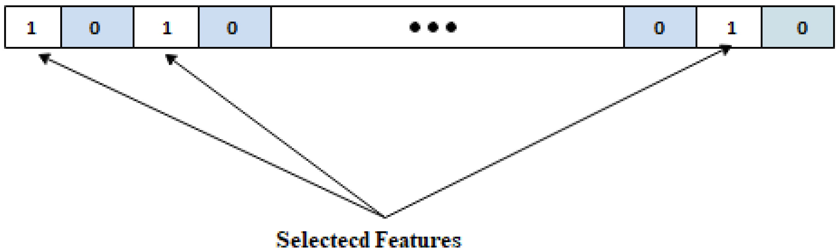
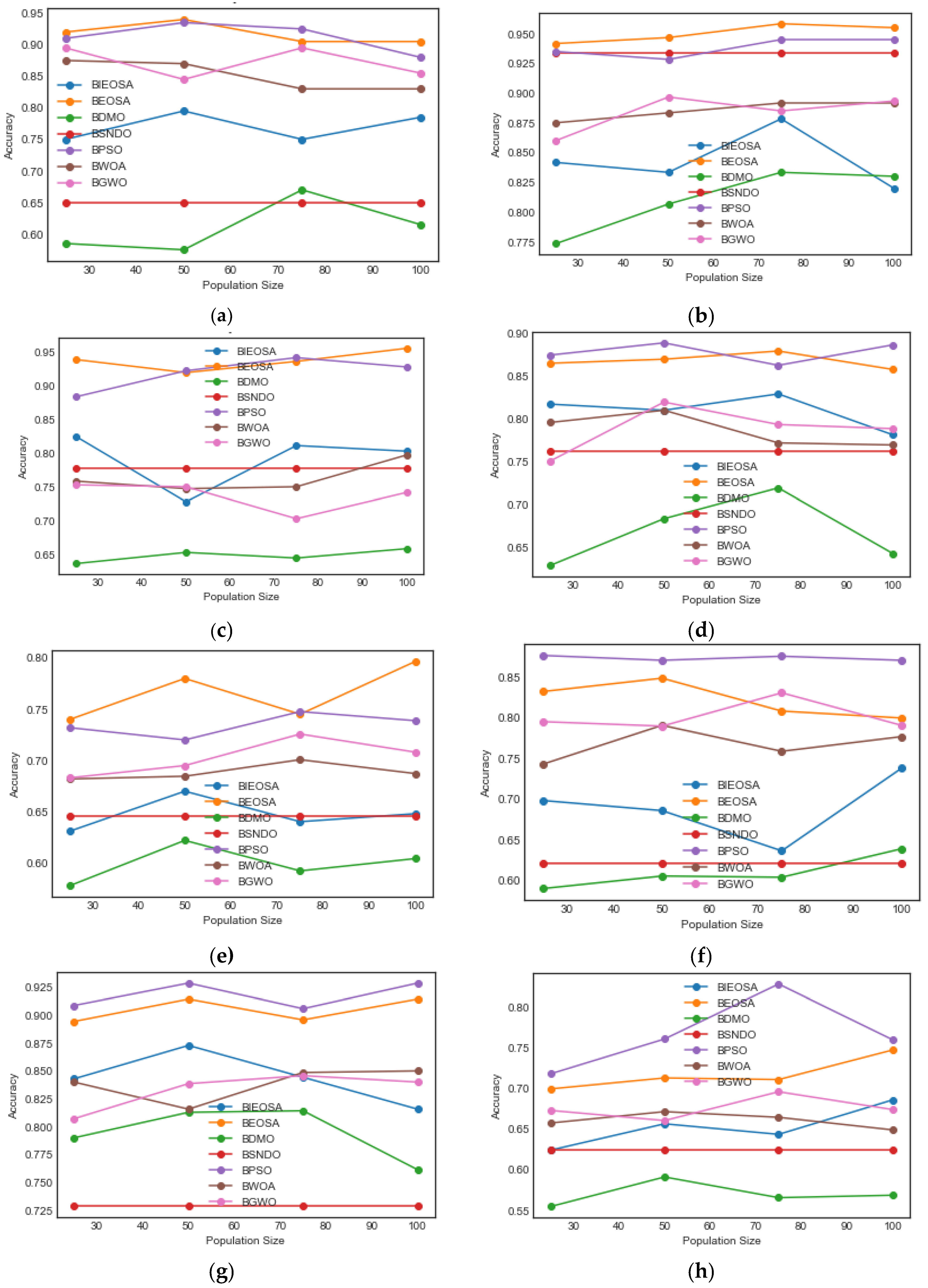
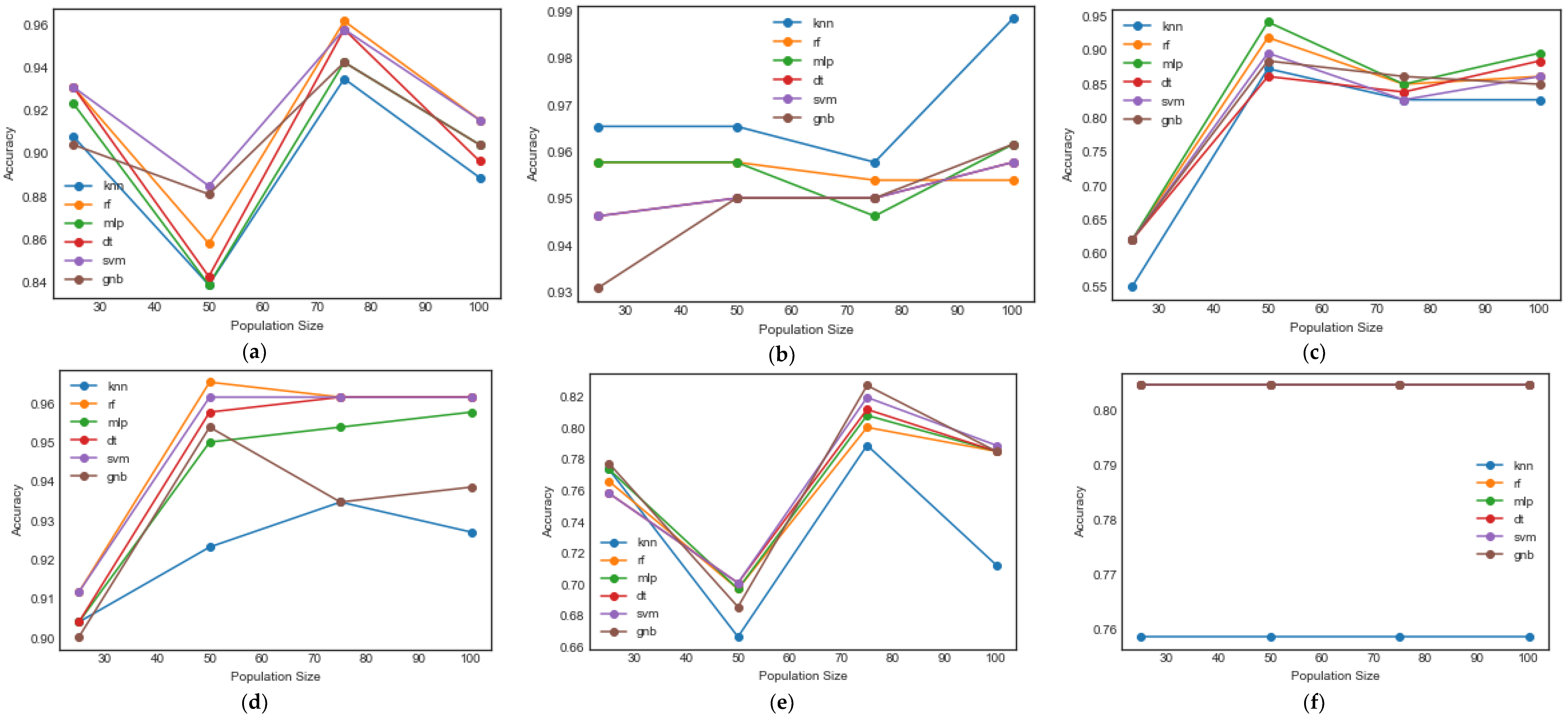
Table 1.
Datasets and their corresponding details, such as the number of features, classes and instances, and a description of each.
Table 1.
Datasets and their corresponding details, such as the number of features, classes and instances, and a description of each.
| Dataset and References | Number of Features | Number of Instances | Number of Class | Description |
|---|---|---|---|---|
| BreastEW | 569 | 30 | 2 | Biology-based and medical-oriented dataset |
| Lung [43] | 3312 | 203 | 5 | Biology-based and medical-oriented dataset |
| CongressEW [44] | 435 | 16 | 2 | Congressional voting dataset |
| Exactly [45] | 1000 | 13 | 2 | Artificial binary classification dataset |
| Iris [46] | 4 | 150 | 2 | Biology-based dataset |
| Exactly2 [45] | 1000 | 13 | 2 | Artificial binary classification dataset |
| HeartEW | 270 | 13 | 2 | Biology-based and medical-oriented dataset |
| Ionosphere [47], | 351 | 34 | 2 | Electromagnetic dataset |
| Prostate | 5966 | 102 | 2 | Biology-based and medical-oriented dataset |
| Lymphography [48] | 148 | 18 | 4 | Biology-based and medical-oriented dataset |
| M-of-n | 1000 | 13 | 2 | Biology-based and medical-oriented dataset |
| Leukemia | 7070 | 72 | 2 | Biology-based and medical-oriented dataset |
| PenglungEW | 325 | 73 | 7 | Biology-based and medical-oriented dataset |
| Sonar | 208 | 60 | 2 | Sonar signal classification dataset |
| SpectEW [49] | 267 | 22 | 2 | Biology-based and medical-oriented dataset |
| Colon | 2000 | 62 | 2 | Biology-based and medical-oriented dataset |
| Tic-tac-toe [50] | 958 | 9 | 2 | Endgame dataset |
| Vote | 300 | 16 | 2 | Electioneering domain |
| Wine [51] | 178 | 13 | 3 | Wine dataset showing the results of analysis of chemicals in wines. |
| Zoo | 101 | 16 | 7 | Biology-based dataset |
| KrVsKpEW | 3196 | 36 | 2 | Game dataset |
| WaveformEW [52] | 5000 | 40 | 3 | A generator dataset generates three classes of waves, with each class sampled at 21 intervals. Additionally, each class is a random convex combining 2 out of 3 base waves. |
Table 2.
Parameters for the BEOSA, BIEOSA, BDMO, BSNDO, BPSO, BWOA, BSFO and BGWO metaheuristic algorithms in this study. N, as used for BDMO and BSNDO, denotes the population size.
Table 2.
Parameters for the BEOSA, BIEOSA, BDMO, BSNDO, BPSO, BWOA, BSFO and BGWO metaheuristic algorithms in this study. N, as used for BDMO and BSNDO, denotes the population size.
| Method | Parameter | Value | Definition |
|---|---|---|---|
| BEOSA | π | 0.1 | Recruitment rate |
| β1, β2, β3 and β4 | 0.1, 0.1, 0.1, and 0.1 | Contact rate of infected individuals, of the host, with the dead and with the recovered individuals | |
| BIEOSA | π | 0.1 | Recruitment rate |
| β1, β2, β3 and β4 | 0.1, 0.1, 0.1, and 0.1 | Contact rate of infected individuals, of the host, with the dead and with the recovered individuals | |
| BDMO | nb | 3 | Number of babysitters |
| na | N- nb | Number of alpha | |
| ns | N- nb | Number of subordinates | |
| peep, | 1, rand (0, 1) | Peep sound, tau operator for fitness evaluation | |
| L | round (0.6*D*nb) | Babysitter exchange parameter | |
| BSNDO | mo | mean(N) | Mean position of the population |
| BPSO | c1, c2 | 2, 2 | Positive learning factors constant 1 and constant 2 |
| W | 0.9 | Initial weight | |
| Vmax | 6 | Maximum velocity vector | |
| BWOA | p, l | [0, 1], [-1, 1] | Random number, random number |
| b | 1 | Shape of spiral | |
| r, C | [0, 1], 2r | Random vector, coefficient vector | |
| BSFO | Pp | 0.1 | Percentage of the sardine population |
| A, | 4, 0.001 | The coefficient for decreasing power attack | |
| BGWO | au | [2,0] |
Table 3.
Results of fitness and cost functions for BWOA, BPSO, BSFO, BGWO, BDMO, BSNDO, BEOSA and BIEOSA on all benchmark datasets.
Table 3.
Results of fitness and cost functions for BWOA, BPSO, BSFO, BGWO, BDMO, BSNDO, BEOSA and BIEOSA on all benchmark datasets.
| Dataset | BWOA | BPSO | BSFO | BGWO | BDMO | BSNDO | BEOSA | BIEOSA | ||||||||
|---|---|---|---|---|---|---|---|---|---|---|---|---|---|---|---|---|
| Fitness | Cost | Fitness | Cost | Fitness | Cost | Fitness | Cost | Fitness | Cost | Fitness | Cost | Fitness | Cost | Fitness | Cost | |
| BreastEW | 0.0307 | 0.9693 | 1.0000 | 0.0000 | 0.0374 | 0.9626 | 0.0564 | 0.9436 | 0.8233 | 0.1767 | 0.9265 | 0.0735 | 0.0404 | 0.9596 | 0.0651 | 0.9349 |
| Lung | 0.0006 | 0.9994 | 0.0516 | 0.9484 | 0.0535 | 0.9465 | 0.0307 | 0.9693 | 0.9729 | 0.0271 | 0.9729 | 0.0271 | 0.0490 | 0.9510 | 0.0492 | 0.9508 |
| CongressEW | 0.0588 | 0.9412 | 0.2175 | 0.7825 | 0.026 | 0.9742 | 0.0259 | 0.9741 | 0.9071 | 0.0929 | 0.9071 | 0.0929 | 0.0575 | 0.9425 | 0.1068 | 0.8932 |
| Exactly | 0.6923 | 0.3077 | 0.4859 | 0.5141 | 0′0147 | 0.9853 | 0.026 | 0.9740 | 0.6923 | 0.3077 | 0.6923 | 0.3077 | 0.2620 | 0.7380 | 0.3553 | 0.6447 |
| Iris | 0.0050 | 0.9950 | 0.6295 | 0.3705 | NA | 1.0000 | 0.0025 | 0.9975 | 0.7005 | 0.2995 | 0.8300 | 0.1700 | 0.0380 | 0.9620 | 0.2030 | 0.7970 |
| Exactly2 | 0.2384 | 0.7616 | 0.2399 | 0.7601 | 0.0355 | 0.9645 | 0.2324 | 0.7676 | 0.6984 | 0.3016 | 0.6984 | 0.3016 | 0.2384 | 0.7616 | 0.2384 | 0.7616 |
| HeartEW | 0.2582 | 0.7418 | 0.4431 | 0.5569 | 0.3744 | 0.6256 | 0.1322 | 0.8678 | 0.5401 | 0.4599 | 0.4859 | 0.5141 | 0.0772 | 0.9228 | 0.2956 | 0.7044 |
| Ionosphere | 0.0734 | 0.9266 | 0.2171 | 0.7829 | 0.1791 | 0.8209 | 0.1335 | 0.8665 | 0.8860 | 0.1140 | 0.0162 | 0.9838 | 0.0722 | 0.9278 | 0.1288 | 0.8712 |
| Prostate | 0.0004 | 0.9996 | 0.0963 | 0.9037 | 0.0064 | 0.9936 | 0.0064 | 0.9936 | 0.9526 | 0.0474 | 0.9526 | 0.0474 | 0.0002 | 0.9998 | 0.0486 | 0.9514 |
| Lymphography | 0.2024 | 0.7976 | 0.3669 | 0.6331 | 0.3647 | 0.6353 | 0.1062 | 0.8938 | 0.5996 | 0.4004 | 0.0380 | 0.9620 | 0.1040 | 0.8960 | 0.3003 | 0.6997 |
| M-of-n | 0.2506 | 0.7494 | 0.6252 | 0.3748 | 0.3678 | 0.6322 | 0.0054 | 0.9946 | 0.7281 | 0.2719 | 0.0046 | 0.9954 | 0.1581 | 0.8419 | 0.3678 | 0.6322 |
| Leukemia | 0.0662 | 0.9338 | 0.0736 | 0.9264 | NA | 1.0000 | 0.0063 | 0.9937 | 0.9297 | 0.0703 | 0.9297 | 0.0703 | 0.0662 | 0.9338 | 0.0042 | 0.9958 |
| PenglungEW | 0.0705 | 0.9295 | 0.0042 | 0.9958 | 0.2065 | 0.7935 | 0.0059 | 0.9941 | 0.6672 | 0.3328 | 0.0013 | 0.9987 | 0.0672 | 0.9328 | 0.2689 | 0.7311 |
| Sonar | 0.0724 | 0.9276 | 0.1194 | 0.8806 | 0.1946 | 0.8054 | 0.1946 | 0.8054 | 0.7626 | 0.2374 | 0.0047 | 0.9953 | 0.0717 | 0.9283 | 0.1889 | 0.8111 |
| SpectEW | 0.1315 | 0.8685 | 0.2223 | 0.7777 | 0.2465 | 0.7535 | 0.1159 | 0.8841 | 0.7764 | 0.2236 | 0.0948 | 0.9052 | 0.1498 | 0.8502 | 0.2433 | 0.7567 |
| Colon | 0.0004 | 0.9996 | 0.3860 | 0.6140 | NA | 1.0000 | 0.0063 | 0.9937 | 0.8449 | 0.1551 | 0.8449 | 0.1551 | 0.0001 | 0.9999 | 0.0776 | 0.9224 |
| Tic-tac-toe | 0.2623 | 0.7377 | 1.0000 | 0.0000 | 0.7635 | 0.2365 | 0.1750 | 0.8250 | 0.6534 | 0.3466 | 0.1647 | 0.8353 | 0.2943 | 0.7057 | 0.3809 | 0.6191 |
| Vote | 0.0013 | 0.9988 | 1.0000 | 0.0000 | 0.1681 | 0.8319 | 0.0203 | 0.9798 | 0.8471 | 0.1529 | 0.0019 | 0.9981 | 0.0545 | 0.9455 | 0.0863 | 0.9138 |
| Wine | 0.0306 | 0.9694 | 0.3865 | 0.6135 | 0.3048 | 0.6952 | 0.0863 | 0.9137 | 0.6685 | 0.3315 | 0.0298 | 0.9702 | 0.0298 | 0.9702 | 0.1131 | 0.8869 |
| Zoo | 0.0520 | 0.9480 | 0.2005 | 0.7995 | 0.1992 | 0.8008 | 0.0545 | 0.9455 | 0.7500 | 0.2500 | 0.7500 | 0.2500 | 0.0533 | 0.9468 | 0.2017 | 0.7983 |
| KrVsKpEW | 0.0612 | 0.9388 | 0.4728 | 0.5272 | 0.3519 | 0.6481 | 0.0348 | 0.9652 | 0.6828 | 0.3172 | 0.0250 | 0.9750 | 0.0382 | 0.9618 | 0.4083 | 0.5917 |
| WaveformEW | 0.2102 | 0.7898 | 0.5468 | 0.4533 | 0.3149 | 0.6851 | 0.1817 | 0.8183 | 0.3394 | 0.6606 | 1.0000 | 0.2431 | 0.7569 | 0.2762 | 0.7238 | |
| Summary | 6 | 6 | 0 | 0 | 0 | 0 | 1 | 1 | 0 | 0 | 8 | 8 | 8 | 8 | 2 | 2 |
Table 4.
Results of the average number of features selected for BWOA, BPSO, BSFO, BGWO, BDMO, BSNDO, BEOSA and BIEOSA on all datasets with population sizes of 25, 50, 75 and 100.
Table 4.
Results of the average number of features selected for BWOA, BPSO, BSFO, BGWO, BDMO, BSNDO, BEOSA and BIEOSA on all datasets with population sizes of 25, 50, 75 and 100.
| Dataset | BWOA | BPSO | BSFO | BGWO | BDMO | BSNDO | BEOSA | BIEOSA | ||||||||||||||||||||||||
|---|---|---|---|---|---|---|---|---|---|---|---|---|---|---|---|---|---|---|---|---|---|---|---|---|---|---|---|---|---|---|---|---|
| Number of Features | Number of Features | Number of Features | Number of Features | Number of Features | Number of Features | Number of Features | Number of Features | |||||||||||||||||||||||||
| 25 | 50 | 75 | 100 | 25 | 50 | 75 | 100 | 25 | 50 | 75 | 100 | 25 | 50 | 75 | 100 | 25 | 50 | 75 | 100 | 25 | 50 | 75 | 100 | 25 | 50 | 75 | 100 | 25 | 50 | 75 | 100 | |
| BreastEW | 17.0 | 17.1 | 17.3 | 18.4 | 1.0 | 1.0 | 1.0 | 1.0 | 10.5 | 10.0 | 11.0 | 11.5 | 20.1 | 18.9 | 18.6 | 16.9 | 7.1 | 8.3 | 5.5 | 5.6 | 3.0 | 3.0 | 3.0 | 3.0 | 7.3 | 10.3 | 9.6 | 8.1 | 7.7 | 5.9 | 10.0 | 8.1 |
| Lung | 1907.2 | 1840.7 | 1693.5 | 1692.5 | 1.0 | 1.0 | 1.0 | 1.0 | NA | NA | NA | NA | 2165.4 | 2180.4 | 2151.1 | 2168.9 | 847.5 | 820.3 | 1161.9 | 971.2 | 2098.4 | 2098.4 | 2098.4 | 2098.4 | 443.7 | 857.4 | 461.9 | 403.9 | 970.4 | 1189.7 | 685.3 | 699.9 |
| CongressEW | 9.4 | 9.8 | 9.1 | 8.9 | 1.0 | 1.0 | 1.0 | 1.0 | 6.7 | 6.6 | 6.0 | 5.8 | 10.1 | 11.2 | 10.2 | 10.2 | 4.7 | 2.4 | 2.9 | 3.2 | 2.4 | 2.4 | 2.4 | 2.4 | 5.9 | 5.7 | 6.4 | 5.3 | 5.7 | 4.6 | 5.1 | 5.9 |
| Exactly | 7.1 | 6.2 | 7.7 | 7.6 | 1.0 | 1.0 | 1.0 | 1.0 | 0.7 | 0.7 | 0.7 | 0.7 | 8.5 | 9.1 | 9.3 | 9.4 | 3.0 | 3.9 | 3.3 | 3.1 | 2.2 | 2.2 | 2.2 | 2.2 | 4.2 | 4.3 | 4.8 | 4.9 | 3.5 | 3.6 | 2.5 | 2.6 |
| Iris | 3.0 | 3.0 | 3.0 | 2.0 | 1.0 | 1.0 | 1.0 | 1.0 | 1.0 | 1.0 | 1.0 | 1.0 | 1.0 | 3.0 | 3.0 | 2.0 | 2.0 | 2.0 | 1.0 | 1.0 | 1.0 | 2.0 | 1.0 | 2.0 | 1.4 | 1.3 | 1.7 | 1.8 | 2.0 | 2.0 | 2.0 | 2.0 |
| Exactly2 | 7.3 | 7.0 | 8.0 | 5.7 | 1.0 | 1.0 | 1.0 | 1.0 | 4.5 | 5.0 | 5.0 | 4.5 | 8.8 | 8.9 | 8.3 | 8.3 | 4.0 | 3.7 | 4.8 | 3.5 | 2.0 | 2.0 | 2.0 | 2.0 | 2.0 | 1.9 | 1.7 | 1.7 | 2.5 | 3.7 | 3.6 | 3.6 |
| HeartEW | 7.1 | 7.5 | 8.2 | 7.7 | 1.0 | 1.0 | 1.0 | 1.0 | 5.0 | 5.0 | 1.0 | 5.0 | 8.7 | 9.5 | 8.3 | 7.5 | 2.8 | 2.8 | 3.7 | 2.9 | 1.0 | 1.0 | 1.0 | 1.0 | 4.3 | 3.1 | 4.8 | 2.6 | 4.3 | 3.7 | 2.7 | 2.8 |
| Ionosphere | 18.6 | 17.2 | 17.6 | 17.2 | 1.0 | 1.0 | 1.0 | 1.0 | 8.0 | 14.0 | 10.0 | 8.0 | 21.9 | 21.8 | 21.1 | 21.5 | 5.0 | 8.8 | 8.3 | 5.5 | 8.4 | 8.4 | 8.4 | 8.4 | 7.3 | 7.1 | 7.6 | 8.4 | 8.0 | 10.2 | 10.6 | 8.2 |
| Prostate | 3274.1 | 3257.7 | 3255.6 | 3286.4 | 1.0 | 1.0 | 1.0 | 1.0 | 3916 | 3916 | 3916 | 3916 | 3937.1 | 3949.7 | 3929.2 | 3927.2 | 2272.8 | 1506.3 | 1685.3 | 1402.8 | 1478.4 | 1478.4 | 1478.4 | 1478.4 | 1326.1 | 941.5 | 895.3 | 682.2 | 1141.5 | 1389.3 | 1437.3 | 1359.3 |
| Lymphography | 12.0 | 10.3 | 10.1 | 9.6 | 1.0 | 1.0 | 1.0 | 1.0 | 9.0 | 9.0 | 9.0 | 5.0 | 11.7 | 12.8 | 12.2 | 11.4 | 3.9 | 4.7 | 5.9 | 3.5 | 1.0 | 1.0 | 1.0 | 1.0 | 7.3 | 6.9 | 7.1 | 7.1 | 4.5 | 5.9 | 6.0 | 5.6 |
| M-of-n | 8.2 | 8.1 | 8.3 | 7.3 | 1.0 | 1.0 | 1.0 | 1.0 | 1.0 | 5.0 | 2.0 | 6.0 | 8.6 | 7.8 | 8.2 | 8.4 | 2.2 | 1.9 | 2.9 | 2.9 | 0.6 | 0.6 | 0.6 | 0.6 | 7.1 | 7.5 | 7.0 | 6.1 | 4.3 | 4.0 | 3.2 | 4.5 |
| Leukemia | 1708.3 | 1719.8 | 1872.7 | 1778.9 | 1.0 | 1.0 | 1.0 | 1.0 | NA | NA | NA | NA | 2340.6 | 2334.1 | 2320.4 | 2337.8 | 1025.2 | 1483.3 | 999.7 | 1194.3 | 928.5 | 928.5 | 928.5 | 928.5 | 253.6 | 110.3 | 121.9 | 50.3 | 1202.4 | 865.7 | 589.7 | 876.0 |
| PenglungEW | 192.0 | 190.0 | 170.0 | 179.0 | 1.0 | 1.0 | 1.0 | 1.0 | 109.0 | 4.0 | 85 | 67 | 207.0 | 193.0 | 212.0 | 213.0 | 176.2 | 103.9 | 189.4 | 23.9 | 142.0 | 144.0 | 124.0 | 170.0 | 46.0 | 134.0 | 35.0 | 40.0 | 24.0 | 122.0 | 92.0 | 158.0 |
| Sonar | 34.6 | 34.0 | 31.6 | 32.1 | 1.0 | 1.0 | 1.0 | 1.0 | 20.0 | 10.0 | 9.0 | 8.0 | 38.2 | 38.5 | 39.6 | 37.9 | 7.3 | 13.0 | 18.6 | 11.1 | 23.0 | 23.0 | 23.0 | 23.0 | 22.4 | 23.7 | 24.3 | 16.5 | 18.8 | 18.5 | 19.3 | 13.9 |
| SpectEW | 12.2 | 13.1 | 12.3 | 10.2 | 1.0 | 1.0 | 1.0 | 1.0 | 3.0 | 6.0 | 4.0 | 9.0 | 13.4 | 13.9 | 15.6 | 13.6 | 5.7 | 10.1 | 6.3 | 8.4 | 3.1 | 3.1 | 3.1 | 3.1 | 7.7 | 9.3 | 7.0 | 7.5 | 7.9 | 5.3 | 5.9 | 6.3 |
| Colon | 1127.0 | 1016.1 | 1066.2 | 1035.0 | 1.0 | 1.0 | 1.0 | 1.0 | NA | NA | NA | NA | 1302.0 | 1303.2 | 1306.3 | 1301.5 | 546.2 | 623.6 | 657.4 | 727.7 | 1374.3 | 1374.3 | 1374.3 | 1374.3 | 338.5 | 286.8 | 197.0 | 157.1 | 384.3 | 632.0 | 472.5 | 316.5 |
| Tic-tac-toe | 4.7 | 4.7 | 5.4 | 4.7 | 1.0 | 1.0 | 1.0 | 1.0 | 3.0 | 3.0 | 4.0 | 1.0 | 5.6 | 6.3 | 6.2 | 6.1 | 2.3 | 2.3 | 1.8 | 2.1 | 1.4 | 1.4 | 1.4 | 1.4 | 5.5 | 5.6 | 5.2 | 6.4 | 2.5 | 2.9 | 3.1 | 2.7 |
| Vote | 8.5 | 9.2 | 8.4 | 7.5 | 1.0 | 1.0 | 1.0 | 1.0 | 1.0 | 1.0 | 1.0 | 1.0 | 10.8 | 11.3 | 11.0 | 10.2 | 3.4 | 4.1 | 4.3 | 3.7 | 7.0 | 7.0 | 7.0 | 7.0 | 5.1 | 5.8 | 5.7 | 5.1 | 3.5 | 4.4 | 5.0 | 4.0 |
| Wine | 7.4 | 8.2 | 8.0 | 7.3 | 1.0 | 1.0 | 1.0 | 1.0 | 3.0 | 1.0 | 3.0 | 5.0 | 7.7 | 8.2 | 8.0 | 7.3 | 3.0 | 3.8 | 3.1 | 2.6 | 2.6 | 2.6 | 2.6 | 2.6 | 5.0 | 4.5 | 4.9 | 5.4 | 4.3 | 3.7 | 3.8 | 3.8 |
| Zoo | 10.1 | 8.6 | 8.8 | 9.3 | 1.0 | 1.0 | 1.0 | 1.0 | 6.0 | 1.0 | 4.0 | 6.0 | 10.9 | 10.6 | 10.0 | 9.3 | 2.4 | 1.8 | 3.9 | 3.3 | 3.0 | 3.0 | 3.0 | 3.0 | 6.8 | 7.7 | 7.3 | 7.6 | 5.1 | 4.6 | 4.5 | 5.6 |
| KrVsKpEW | 19.0 | 23.0 | 21.0 | 26.0 | 1.0 | 1.0 | 1.0 | 1.0 | 10.0 | 10.0 | 10.0 | 10.0 | 27.0 | 22.0 | 27.0 | 25.0 | 6.1 | 2.4 | 4.2 | 5.7 | 2.4 | 2.4 | 2.4 | 2.4 | 22.6 | 17.4 | 20.9 | 21.1 | 8.0 | 10.8 | 8.8 | 12.8 |
| WaveformEW | 25.8 | 26.1 | 27.0 | 25.7 | 1.0 | 1.0 | 1.0 | 1.0 | NA | NA | NA | NA | 27.0 | 27.0 | 27.0 | 25.0 | 14.0 | 6.9 | 1.0 | 2.1 | 20.0 | 20.0 | 25.0 | 24.0 | 25.0 | 20.0 | 26.0 | 14.0 | 11.0 | 18.0 | 4.0 | 12.8 |
Table 5.
Comparative analysis of classification accuracy obtained for BWOA, BPSO, BSFO, BGWO, BDMO, BSNDO, BEOSA and BIEOSA on all datasets using population sizes of 25, 50, 75, and 100.
Table 5.
Comparative analysis of classification accuracy obtained for BWOA, BPSO, BSFO, BGWO, BDMO, BSNDO, BEOSA and BIEOSA on all datasets using population sizes of 25, 50, 75, and 100.
| Dataset | BWOA | BPSO | BSFO | BGWO | BDMO | BSNDO | BEOSA | BIEOSA | ||||||||||||||||||||||||
|---|---|---|---|---|---|---|---|---|---|---|---|---|---|---|---|---|---|---|---|---|---|---|---|---|---|---|---|---|---|---|---|---|
| Accuracy | Accuracy | Accuracy | Accuracy | Accuracy | Accuracy | Accuracy | Accuracy | |||||||||||||||||||||||||
| 25 | 50 | 75 | 100 | 25 | 50 | 75 | 100 | 25 | 50 | 75 | 100 | 25 | 50 | 75 | 100 | 25 | 50 | 75 | 100 | 25 | 50 | 75 | 100 | 25 | 50 | 75 | 100 | 25 | 50 | 75 | 100 | |
| BreastEW | 0.9175 | 0.9351 | 0.9184 | 0.9219 | 0.9368 | 0.9439 | 0.9535 | 0.9421 | 0.8070 | 0.9035 | 0.7456 | 0.8596 | 0.9272 | 0.9123 | 0.9132 | 0.9140 | 0.8921 | 0.8526 | 0.7544 | 0.7912 | 0.6930 | 0.6930 | 0.6930 | 0.6930 | 0.9430 | 0.9456 | 0.9377 | 0.9430 | 0.8974 | 0.8807 | 0.9149 | 0.9026 |
| Lung | 0.9512 | 0.9659 | 0.9512 | 0.9610 | 0.9829 | 0.9805 | 0.9780 | 0.9902 | NA | NA | NA | NA | 0.9512 | 0.9390 | 0.9537 | 0.9512 | 0.9098 | 0.9073 | 0.9049 | 0.9268 | 0.9268 | 0.9268 | 0.9268 | 0.9268 | 0.9829 | 0.9854 | 0.9854 | 0.9829 | 0.9537 | 0.9415 | 0.9463 | 0.9439 |
| CongressEW | 0.9126 | 0.9333 | 0.9310 | 0.9046 | 0.9540 | 0.9678 | 0.9609 | 0.9621 | 0.5517 | 0.8736 | 0.8276 | 0.8276 | 0.9264 | 0.9195 | 0.9391 | 0.9333 | 0.8149 | 0.6793 | 0.7483 | 0.7713 | 0.8276 | 0.8276 | 0.8276 | 0.8276 | 0.9621 | 0.9563 | 0.9644 | 0.9667 | 0.8989 | 0.9103 | 0.8862 | 0.9034 |
| Exactly | 0.6575 | 0.6715 | 0.6645 | 0.6490 | 0.7180 | 0.7610 | 0.8285 | 0.7600 | 0.6900 | 0.6150 | 0.6900 | 0.6900 | 0.6730 | 0.6605 | 0.6960 | 0.6740 | 0.5545 | 0.5910 | 0.5655 | 0.5685 | 0.6250 | 0.6250 | 0.6250 | 0.6250 | 0.6995 | 0.7130 | 0.7110 | 0.7475 | 0.6240 | 0.6565 | 0.6435 | 0.6860 |
| Iris | 0.9333 | 1.0000 | 0.9333 | 0.9000 | 0.9667 | 0.9333 | 1.0000 | 1.0000 | 0.9667 | 0.966667 | 0.9667 | 0.9667 | 0.7333 | 1.0000 | 0.9333 | 1.0000 | 0.9667 | 0.8333 | 0.4000 | 0.5667 | NA | NA | NA | NA | 1.0000 | 1.0000 | 1.0000 | 0.9667 | 0.7333 | 0.9333 | 0.8333 | 0.8000 |
| Exactly2 | 0.7070 | 0.7275 | 0.7210 | 0.7345 | 0.7610 | 0.7620 | 0.7610 | 0.7660 | 0.6250 | 0.7350 | 0.7300 | 0.7300 | 0.7175 | 0.7120 | 0.7115 | 0.7150 | 0.6640 | 0.6365 | 0.6875 | 0.6260 | 0.5900 | 0.5900 | 0.5900 | 0.5900 | 0.7620 | 0.7625 | 0.7625 | 0.7610 | 0.7495 | 0.7435 | 0.7375 | 0.7325 |
| HeartEW | 0.6537 | 0.6296 | 0.6667 | 0.6963 | 0.7833 | 0.8019 | 0.7852 | 0.8019 | 0.7037 | 0.6111 | 0.5185 | 0.7222 | 0.6833 | 0.6556 | 0.6241 | 0.6963 | 0.5481 | 0.5722 | 0.5556 | 0.5315 | 0.4815 | 0.4815 | 0.4815 | 0.4815 | 0.7741 | 0.7759 | 0.8074 | 0.8074 | 0.6907 | 0.6593 | 0.6870 | 0.6685 |
| Ionosphere | 0.8400 | 0.8157 | 0.8486 | 0.8500 | 0.9086 | 0.9286 | 0.9057 | 0.9286 | 0.9000 | 0.8429 | 0.8143 | 0.8286 | 0.8071 | 0.8386 | 0.8457 | 0.8400 | 0.7900 | 0.8129 | 0.8143 | 0.7614 | 0.7286 | 0.7286 | 0.7286 | 0.7286 | 0.8943 | 0.9143 | 0.8957 | 0.9143 | 0.8429 | 0.8729 | 0.8443 | 0.8157 |
| Prostate | 0.9333 | 0.9286 | 0.9476 | 0.9762 | 1.0000 | 1.0000 | 1.0000 | 1.0000 | 1.0000 | 1.0000 | 1 | 1.0000 | 0.9571 | 0.9810 | 0.9429 | 0.9095 | 0.7857 | 0.7524 | 0.7714 | 0.7476 | 0.9048 | 0.9048 | 0.9048 | 0.9048 | 0.9905 | 1.0000 | 0.9952 | 1.0000 | 0.9095 | 0.8857 | 0.8857 | 0.8286 |
| Lymphography | 0.8000 | 0.8000 | 0.7667 | 0.6667 | 0.8533 | 0.8733 | 0.8800 | 0.8700 | 0.6667 | 0.7333 | 0.7667 | 0.6333 | 0.7500 | 0.7300 | 0.7333 | 0.7633 | 0.5633 | 0.5567 | 0.6267 | 0.5233 | 1.0000 | 0.9333 | 1.0000 | 0.9667 | 0.8233 | 0.8567 | 0.8500 | 0.8400 | 0.6567 | 0.6800 | 0.6933 | 0.6900 |
| M-of-n | 0.7425 | 0.7905 | 0.7585 | 0.7765 | 0.8765 | 0.8705 | 0.8755 | 0.8705 | 0.6300 | 0.6900 | 0.6600 | 0.7400 | 0.7950 | 0.7895 | 0.8305 | 0.7905 | 0.5895 | 0.6050 | 0.6035 | 0.6385 | 0.6200 | 0.6200 | 0.6200 | 0.6200 | 0.8320 | 0.8485 | 0.8080 | 0.7995 | 0.6980 | 0.6855 | 0.6360 | 0.7375 |
| Leukemia | 0.9600 | 0.9467 | 0.9533 | 0.9667 | 0.9867 | 0.9933 | 0.9867 | 1.0000 | NA | NA | NA | NA | 0.9800 | 0.9667 | 0.9867 | 0.9800 | 0.9133 | 0.9200 | 0.8933 | 0.9000 | 0.8667 | 0.8667 | 0.8667 | 0.8667 | 1.0000 | 0.9933 | 0.9800 | 0.9933 | 0.9133 | 0.9600 | 0.9600 | 0.9800 |
| PenglungEW | 0.8667 | 0.8000 | 0.8000 | 0.8667 | 0.8667 | 0.8000 | 0.8000 | 1.0000 | 0.8000 | 0.4000 | 0.9333 | 0.6667 | 0.8000 | 0.8000 | 0.8667 | 0.8667 | 0.7333 | 0.7333 | 0.6667 | 0.4667 | 0.6667 | 0.8000 | 0.7333 | 0.9333 | 0.9333 | 0.8000 | 0.8667 | 0.8667 | 0.7333 | 1.0000 | 0.8000 | 0.6667 |
| Sonar | 0.7952 | 0.8095 | 0.7714 | 0.7690 | 0.8738 | 0.8881 | 0.8619 | 0.8857 | 0.7143 | 0.7857 | 0.6429 | 0.6905 | 0.7500 | 0.8190 | 0.7929 | 0.7881 | 0.6286 | 0.6833 | 0.7190 | 0.6429 | 0.7619 | 0.7619 | 0.7619 | 0.7619 | 0.8643 | 0.8690 | 0.8786 | 0.8571 | 0.8167 | 0.8095 | 0.8286 | 0.7810 |
| SpectEW | 0.7759 | 0.8037 | 0.8037 | 0.8167 | 0.8370 | 0.8463 | 0.8333 | 0.8463 | 0.7963 | 0.7963 | 0.7963 | 0.7593 | 0.7963 | 0.8148 | 0.7852 | 0.8111 | 0.6963 | 0.7278 | 0.7296 | 0.7352 | 0.7407 | 0.7407 | 0.7407 | 0.7407 | 0.8500 | 0.8444 | 0.8259 | 0.8444 | 0.7833 | 0.8130 | 0.7870 | 0.8037 |
| Colon | 0.9538 | 0.9923 | 0.9077 | 0.9077 | 1.0000 | 1.0000 | 1.0000 | 1.0000 | NA | NA | NA | NA | 0.9385 | 0.9769 | 0.9846 | 0.9154 | 0.7538 | 0.7231 | 0.6846 | 0.7154 | 0.8462 | 0.8462 | 0.8462 | 0.8462 | 1.0000 | 1.0000 | 1.0000 | 1.0000 | 0.8308 | 0.8769 | 0.8692 | 0.8923 |
| Tic-tac-toe | 0.6818 | 0.6844 | 0.7005 | 0.6870 | 0.7318 | 0.7198 | 0.7474 | 0.7385 | 0.6198 | 0.5417 | 0.6979 | 0.6510 | 0.6828 | 0.6948 | 0.7255 | 0.7078 | 0.5776 | 0.6219 | 0.5922 | 0.6042 | 0.6458 | 0.6458 | 0.6458 | 0.6458 | 0.7396 | 0.7797 | 0.7448 | 0.7964 | 0.6307 | 0.6698 | 0.6401 | 0.6479 |
| Vote | 0.8750 | 0.8833 | 0.8917 | 0.8917 | 0.9350 | 0.9283 | 0.9450 | 0.9450 | 0.8500 | 0.8500 | 0.8167 | 0.8500 | 0.8600 | 0.8967 | 0.8850 | 0.8933 | 0.7733 | 0.8067 | 0.8333 | 0.8300 | 0.9333 | 0.9333 | 0.9333 | 0.9333 | 0.9417 | 0.9467 | 0.9583 | 0.9550 | 0.8417 | 0.8333 | 0.8783 | 0.8200 |
| Wine | 0.7306 | 0.7083 | 0.7472 | 0.7639 | 0.9111 | 0.9028 | 0.9278 | 0.8889 | 0.8889 | 0.6111 | 0.6667 | 0.7222 | 0.7722 | 0.7389 | 0.7833 | 0.7639 | 0.6361 | 0.6528 | 0.6444 | 0.6583 | 0.7222 | 0.7222 | 0.7222 | 0.7222 | 0.9389 | 0.9194 | 0.9361 | 0.9556 | 0.8250 | 0.7278 | 0.8111 | 0.8028 |
| Zoo | 0.8750 | 0.8700 | 0.8300 | 0.8300 | 0.9100 | 0.9350 | 0.9250 | 0.8800 | 0.9000 | 0.4000 | 0.6000 | 0.9000 | 0.8950 | 0.8450 | 0.8950 | 0.8550 | 0.5850 | 0.5750 | 0.6700 | 0.6150 | 0.6500 | 0.6500 | 0.6500 | 0.6500 | 0.9200 | 0.9400 | 0.9050 | 0.9050 | 0.7500 | 0.7950 | 0.7500 | 0.7850 |
| KrVsKpEW | 0.8513 | 0.8482 | 0.9468 | 0.9703 | 0.9703 | 0.9656 | 0.960876 | 0.9671 | 0.6166 | 0.6964 | 0.6416 | 0.7230 | 0.9218 | 0.7418 | 0.8451 | 0.9437 | 0.5604 | 0.5133 | 0.5351 | 0.5535 | 0.6729 | 0.6729 | 0.6729 | 0.6729 | 0.8919 | 0.8568 | 0.9103 | 0.8865 | 0.6501 | 0.6962 | 0.6851 | 0.7351 |
| WaveformEW | 0.7509 | 0.7769 | 0.7912 | 0.7639 | 0.8154 | 0.8241 | 0.8295 | 0.8021 | NA | NA | NA | NA | 0.7743 | 0.7582 | 0.7788 | 0.7913 | 0.3550 | 0.4640 | 0.4680 | 0.6060 | NA | NA | NA | NA | 0.8065 | 0.7973 | 0.7919 | 0.7900 | 0.7038 | 0.6119 | 0.6025 | 0.6222 |
| Summary | 0 | 9 | 1 | 10 | 2 | 3 | 5 | 10 | 2 | 6 | 2 | 5 | 2 | 3 | 9 | 5 | 5 | 5 | 6 | 5 | 0 | 0 | 1 | 19 | 3 | 3 | 6 | 9 | 5 | 7 | 5 | 5 |
Table 6.
The classification accuracy, precision, recall, F1-score and area under curve (AUC) report for the M-of-n datasets using KNN, random forest (RF), MLP, Decision Tree (DTree), SVM, and Gaussian naïve Bayes (GNB) classifiers on the BWOA, BPSO, BSFO, BGWO, BDMO, BSNDO, BEOSA and BIEOSA algorithms.
| Algorithm | Classifier | Accuracy | Precision | Recall | F1-Score | AUC |
|---|---|---|---|---|---|---|
| BWOA | KNN | 0.665 | 0.7 | 0.785714 | 0.733333 | 0.770667 |
| RF | 0.71 | 0.714286 | 0.666667 | 0.666667 | 0.805333 | |
| MLP | 0.685 | 0.666667 | 0.8 | 0.727273 | 0.821333 | |
| DTree | 0.72 | 0.8 | 0.533333 | 0.64 | 0.766667 | |
| SVM | 0.71 | 0.777778 | 0.6 | 0.642857 | 0.826667 | |
| GNB | 0.72 | 0.714286 | 0.666667 | 0.689655 | 0.832 | |
| BPSO | KNN | 0.905 | 0.846154 | 0.866667 | 0.785714 | 0.90522 |
| RF | 0.99 | 0.923077 | 0.866667 | 0.857143 | 0.976648 | |
| MLP | 1 | 1 | 1 | 1 | 1 | |
| DTree | 0.79 | 0.818182 | 0.666667 | 0.714286 | 0.741333 | |
| SVM | 1 | 1 | 1 | 1 | 1 | |
| GNB | 0.955 | 1 | 0.8 | 0.888889 | 1 | |
| BSFO | KNN | 0.69 | 0.529412 | 0.6 | 0.5625 | 0.741333 |
| RF | 0.725 | 0.666667 | 0.6 | 0.56 | 0.704 | |
| MLP | 0.725 | 0.857143 | 0.533333 | 0.551724 | 0.74 | |
| DTree | 0.74 | 0.916667 | 0.733333 | 0.814815 | 0.898667 | |
| SVM | 0.74 | 0.916667 | 0.733333 | 0.814815 | 0.850667 | |
| GNB | 0.74 | 0.916667 | 0.733333 | 0.814815 | 0.882667 | |
| BGWO | KNN | 0.675 | 0.8 | 0.571429 | 0.666667 | 0.826923 |
| RF | 0.71 | 0.7 | 0.666667 | 0.666667 | 0.834667 | |
| MLP | 0.705 | 0.727273 | 0.533333 | 0.615385 | 0.805333 | |
| DTree | 0.755 | 0.857143 | 0.6 | 0.642857 | 0.8 | |
| SVM | 0.755 | 0.857143 | 0.733333 | 0.758621 | 0.806667 | |
| GNB | 0.755 | 0.777778 | 0.666667 | 0.689655 | 0.846154 | |
| BDMO | KNN | 0.6 | 0.692308 | 0.866667 | 0.684211 | 0.821333 |
| RF | 0.725 | 0.705882 | 0.866667 | 0.75 | 0.889333 | |
| MLP | 0.725 | 0.705882 | 0.8 | 0.75 | 0.881333 | |
| DTree | 0.725 | 0.75 | 0.533333 | 0.615385 | 0.817333 | |
| SVM | 0.725 | 0.75 | 0.533333 | 0.615385 | 0.897333 | |
| GNB | 0.725 | 0.75 | 0.866667 | 0.774194 | 0.865333 | |
| BSNDO | KNN | 1 | 0.909091 | 0.866667 | 0.866667 | 0.970667 |
| RF | 1 | 1 | 1 | 1 | 1 | |
| MLP | 1 | 1 | 1 | 1 | 1 | |
| DTree | 0.775 | 1 | 0.533333 | 0.666667 | 0.805333 | |
| SVM | 1 | 1 | 1 | 1 | 1 | |
| GNB | 0.96 | 1 | 1 | 1 | 1 | |
| BEOSA | KNN | 0.815 | 0.866667 | 0.928571 | 0.896552 | 0.98489 |
| RF | 0.835 | 1 | 0.928571 | 0.896552 | 0.95467 | |
| MLP | 0.84 | 0.9 | 0.928571 | 0.896552 | 0.971154 | |
| DTree | 0.795 | 0.9 | 0.714286 | 0.769231 | 0.896978 | |
| SVM | 0.845 | 0.875 | 1 | 0.933333 | 0.993132 | |
| GNB | 0.83 | 0.928571 | 0.928571 | 0.928571 | 0.995879 | |
| BIEOSA | KNN | 0.935 | 1 | 0.866667 | 0.928571 | 1 |
| RF | 0.665 | 0.538462 | 0.5 | 0.518519 | 0.748626 | |
| MLP | 0.67 | 0.583333 | 0.466667 | 0.482759 | 0.712912 | |
| DTree | 0.67 | 0.545455 | 0.533333 | 0.5 | 0.717033 | |
| SVM | 0.67 | 0.7 | 0.533333 | 0.583333 | 0.843407 | |
| GNB | 0.67 | 1 | 0.666667 | 0.571429 | 0.769231 |
Table 7.
Comparative analysis of the computational times of BWOA, BPSO, BSFO, BGWO, BDMO, BSNDO, BEOSA, and BIEOSA.
Table 7.
Comparative analysis of the computational times of BWOA, BPSO, BSFO, BGWO, BDMO, BSNDO, BEOSA, and BIEOSA.
| Dataset | BWOA | BPSO | BSFO | BGWO | BDMO | BSNDO | BEOSA | BIEOSA |
|---|---|---|---|---|---|---|---|---|
| BreastEW | 2863.07 | 5716.95 | 15,231.68 | 3284.61 | 4693.94 | 0.05 | 7755.12 | 7143.08 |
| Lung | 10,836.27 | 6407.44 | NA | 13,519.02 | 21,901.97 | 0.06 | 27,005.21 | 27,469.88 |
| CongressEW | 2494.41 | 3293.75 | 21,216.45 | 2911.41 | 3167.04 | 0.05 | 3681.29 | 3439.88 |
| Exactly | 4238.07 | 5576.70 | 37,823.17 | 4967.03 | 5139.55 | 0.05 | 6135.80 | 5239.17 |
| Iris | 1539.72 | 1569.79 | 0.0300 | 1248.06 | 2454.02 | 0.05 | 3638.87 | 4367.40 |
| Exactly2 | 4894.75 | 5460.21 | 84,742.30 | 5886.60 | 5831.48 | 0.05 | 5629.12 | 5949.60 |
| HeartEW | 5991.47 | 6180.32 | 11,961.87 | 6103.14 | 4953.76 | 0.05 | 8289.17 | 7775.06 |
| Ionosphere | 2425.15 | 5192.26 | 26,648.48 | 2711.81 | 4576.30 | 0.06 | 6795.18 | 5838.63 |
| Prostate | 13,996.86 | 23,715.34 | 0.0500 | 19,962.22 | 18,691.10 | 0.05 | 14,753.88 | 14,729.31 |
| Lymphography | 7088.64 | 4101.17 | 15,660.77 | 3363.44 | 4113.92 | 24,995.09 | 6342.72 | 6345.36 |
| M-of-n | 3377.35 | 4705.02 | 56,589.18 | 4243.87 | 4042.42 | 0.05 | 5927.31 | 4770.37 |
| Leukemia | 12,557.96 | 15,367.75 | NA | 15,879.91 | 14,626.92 | 0.05 | 10,973.17 | 13,082.37 |
| PenglungEW | 972.86 | 1186.14 | 7022.13 | 1027.13 | 1057.12 | 1613.04 | 1570.83 | 1238.32 |
| Sonar | 2478.74 | 3265.90 | 23,013.84 | 2694.13 | 4308.82 | 0.06 | 4640.60 | 4789.33 |
| SpectEW | 2809.20 | 3386.75 | 15,919.29 | 3107.25 | 3314.52 | 0.04 | 4389.90 | 4118.12 |
| Colon | 9003.78 | 10,541.57 | NA | 11,003.80 | 10,026.80 | 0.06 | 8971.40 | 9562.65 |
| Tic-tac-toe | 7769.29 | 9578.16 | 54,646.60 | 8591.51 | 7463.63 | 0.05 | 13,032.30 | 10,677.70 |
| Vote | 2430.62 | 2837.52 | 24,196.79 | 2561.77 | 2947.24 | 0.05 | 4046.51 | 4197.18 |
| Wine | 2774.64 | 4566.93 | 19,463.48 | 3309.42 | 5377.52 | 0.05 | 7005.92 | 8468.67 |
| Zoo | 2013.56 | 2427.55 | 8370.56 | 2118.25 | 2465.75 | 0.05 | 3384.51 | 3437.60 |
| KrVsKpEW | 8482.48 | 17,028.06 | 173,356.6 | 12,685.90 | 20,658.05 | 0.07 | 25,079.98 | 18,698.16 |
| WaveformEW | 17,449.58 | 32,664.62 | NA | 21,421.47 | 22,591.37 | NA | 26,812.95 | 27,680.63 |
Publisher’s Note: MDPI stays neutral with regard to jurisdictional claims in published maps and institutional affiliations. |
© 2022 by the authors. Licensee MDPI, Basel, Switzerland. This article is an open access article distributed under the terms and conditions of the Creative Commons Attribution (CC BY) license (https://creativecommons.org/licenses/by/4.0/).
Share and Cite
MDPI and ACS Style
Akinola, O.; Oyelade, O.N.; Ezugwu, A.E. Binary Ebola Optimization Search Algorithm for Feature Selection and Classification Problems. Appl. Sci. 2022, 12, 11787. https://0-doi-org.brum.beds.ac.uk/10.3390/app122211787
AMA Style
Akinola O, Oyelade ON, Ezugwu AE. Binary Ebola Optimization Search Algorithm for Feature Selection and Classification Problems. Applied Sciences. 2022; 12(22):11787. https://0-doi-org.brum.beds.ac.uk/10.3390/app122211787
Chicago/Turabian StyleAkinola, Olatunji, Olaide N. Oyelade, and Absalom E. Ezugwu. 2022. "Binary Ebola Optimization Search Algorithm for Feature Selection and Classification Problems" Applied Sciences 12, no. 22: 11787. https://0-doi-org.brum.beds.ac.uk/10.3390/app122211787
Note that from the first issue of 2016, this journal uses article numbers instead of page numbers. See further details here.