Variable Neighborhood Search for the Two-Echelon Electric Vehicle Routing Problem with Time Windows

Abstract

Increasing environmental concerns and legal regulations have led to the development of sustainable technologies and systems in logistics, as in many fields. The adoption of multi-echelon distribution networks and the use of environmentally friendly vehicles in freight distribution have become major concepts for reducing the negative impact of urban transportation activities. In this line, the present paper proposes a two-echelon electric vehicle routing problem. In the first echelon of the distribution network, products are transported from central warehouses to satellites located in the surroundings of cities. This is achieved by means of large conventional trucks. Subsequently, relatively smaller-sized electric vehicles distribute these products from the satellites to demand points/customers located in the cities. The proposed problem also takes into account the limited driving range of electric vehicles that need to be recharged at charging stations when necessary. In addition, the proposed problem considers time window constraints for the delivery of products to customers. A mixed-integer linear programming formulation is developed and small-sized instances are solved using CPLEX. Furthermore, we propose a constructive heuristic based on a modified Clarke and Wright savings heuristic. The solutions of this heuristic serve as initial solutions for a variable neighborhood search metaheuristic. The numerical results show that the variable neighborhood search matches CPLEX in the context of small problems. Moreover, it consistently outperforms CPLEX with the growing size and difficulty of problem instances.

1. Introduction

After the industrial revolution, the increasing consumption of fossil fuels caused numerous environmental and socioeconomic problems. In this context, it is considered a prime objective to replace fossil fuel technologies in many sectors with more sustainable technologies in order to reduce the amount of carbon dioxide released into the atmosphere. Increasing environmental and economic concerns and the decisions taken by states to reduce our dependence on fossil fuels have led to an acceleration of research and development activities in this area. This also holds for the logistics sector, where new regulations are introduced in order to reduce environmental problems. One of the most recent regulations in this field is the decision approved by the European Parliament on 18 February 2019, stating that the emissions of new trucks will need to be 30% lower in 2030 compared to 2019 emissions data [1].

In this context, sustainable city logistics emerged as a concept for reducing the negative impact of urban transportation activities on society, the environment and the economy. Sustainable city logistics is characterized by using environmentally friendly vehicles for freight distribution and designing multi-tier transportation structures to eliminate problems caused by freight vehicles operating in cities. A growing number of logistics and e-commerce companies make use of environmentally friendly electric vehicles for distribution in urban areas due to their low noise and zero exhaust emissions; see, for example, [2]. Despite these advantages, the en-route charging necessity of electric vehicles due to a limited driving range produces new difficulties for the planning and managing of logistics activities. In fact, the ability to derive optimal charging plans for electric vehicles taking into account the total time requirements and route distances is essential.

In this study, the issue of sustainable city logistics is addressed by means of a new variant of the classical vehicle routing problem: the two-echelon electric vehicle routing problem with time windows (2E-EVRP-TW). In two-echelon distribution networks, large trucks transport products from central warehouses to satellites in the surrounding areas of cities. Subsequently, smaller vehicles distribute goods from these satellites to customers located in the cities. Electric vehicles are preferably used in the second echelon of such a distribution network, as they are less noisy and have no exhaust emissions. In other words, two-echelon distribution networks are advantageous for preventing large trucks entering the cities and, in this way, reducing urban traffic jams, noise, and pollution. In addition to these features, our 2E-EVRP-TW problem also considers time window (TW) constraints for the delivery of goods to customers. Note that time windows can be used to control the visiting times of the customers, which might be regulated by local jurisdictions, but also by the customers themselves.

1.1. Our Contribution

First, we define the 2E-EVRP-TW problem by means of a three-index node-based mixed-integer linear programming (MILP) model. Any general-purpose MILP solver, such as CPLEX or Gurobi, may be used to solve this model. However, due to the multi-tier structure of the distribution network, the limited driving range of electric vehicles, and the time window constraints, the 2E-EVRP-TW problem is rather complex. In fact, our computational experiments show that CPLEX is only able to solve small-sized problems to optimality. Therefore, we also developed a variable neighborhood search (VNS) approach to solve the problem. In addition, we developed an initial solution generation method based on Clarke and Wright’s savings algorithm [3], considering 2E-EVRP-TW assumptions and characteristics. The VNS approach makes use of this heuristic to obtain an initial solution.

VNS provides a powerful search performance by systematically changing neighborhood structures (shaking) to avoid getting stuck in local optima and by intensifying the search in the vicinity of the incumbent solution by applying local search. In addition to the classical shaking and local search operators, we also utilize large neighborhood search (LNS) operators known as “destroy and repair”, resp. “removal and insertion”, to enhance the performance of VNS. In this context, note that, since (1) the problem dimension of the first echelon is much smaller than that of the second echelon and (2) the first echelon does not include any constraint, it can easily be solved using a savings heuristic. Therefore, whenever the solution for the second echelon changes, the first echelon tours are generated again by utilizing our Clarke and Wright savings heuristic.

Finally, a last contribution concerns the generation of new problem-specific benchmark sets. This was necessary due to the lack of an available benchmark set for the 2E-EVRP-TW problem.

1.2. Organization of the Paper

The rest of this paper is organized as follows: Section 2 presents the related literature. A formal description of the new 2E-EVRP-TW problem, together with a mixed-integer linear programming model, is provided in Section 3. The proposed solution approach is described in Section 4. Section 5 reports computational experiments, and finally, Section 6 outlines our conclusions and future research directions.

2. Related Literature

Recent decades have witnessed considerable research efforts concerning the vehicle routing problem and its variations. Researchers and practitioners have put great effort into modeling and designing efficient routing strategies considering requirements and conditions that arise in real-life scenarios. Various extensions of vehicle routing problems as well as recent advances and challenges are defined and presented in [4,5]. Moreover, a broad taxonomy and a classification of publications available in the VRP literature are provided in [6]. Apart from introducing new problem variations, researchers also focused on developing solution methodologies to solve already existing problem extensions efficiently. A taxonomic review of metaheuristic solution approaches for vehicle routing problems and their variations is presented in [7]. The problem we address in this study combines two main research lines: the one on electric vehicle routing problems (EVRPs) and the one on two-echelon vehicle routing problems (2E-VRPs). Therefore, before presenting works related to our 2E-EVRP-TW problem, we will first summarize the literature on the EVRP and on the 2E-VRP.

Driven by environmental considerations and a growing interest in the use of alternative fuel in logistics, the related literature has focused on developing optimal routing plans considering the limited driving range and en-route charging necessity of electric vehicles. Respective publications either call the tackled problem an EVRP or, more generally, a green vehicle routing problem. A systematic review of green vehicle routing problems is presented in [8,9]. The study presented in [10] is regarded as the pioneering work that introduced route optimization of rechargeable vehicles to the literature. After this preliminary work, several researchers presented variations of electric vehicle routing problems together with solution methodologies. Erdoğan et al. [11] proposed a mixed-integer programming model as well as two heuristic solution techniques for the generation of routing plans for alternative fueling vehicles. Schneider et al. [12] extended the EVRP by including time window constraints into the model. Moreover, they proposed a metaheuristic algorithm based on VNS and tabu search (TS). Aiming to develop more realistic models and applications, Felipe et al. [13] and Keskin and Çatay [14] analyzed and utilized multiple charging technologies with regard to different charging speeds and the partial recharging of electric vehicles. Moreover, Montoya et al. [15] introduced a new model that takes into account the non-linear charging time of batteries. They reported that the time spent for charging batteries is non-linear, and ignoring this fact may cause the generation of infeasible and/or costly solutions. Sadati and Çatay [16] recently introduced a multi-depot green vehicle routing problem and developed a mixed-integer linear programming model. They proposed a solution method based on VNS and TS and reported on the computational properties of the algorithm. Duman et al. [17] proposed exact and heuristic algorithms based on branch-and-price-and-cut and on column generation to solve the EVRP with TWs.

After Crainic et al. [18] introduced the concept of two echelons in the context of the 2E-VRP as a new concept to the literature, this line of research developed into one of the most popular ones in the context of urban freight transportation [19]. The idea of developing sustainable cities and transportation systems further increases the interest in this field of research. Perboli et al. [20] proposed a mathematical model and math-based heuristics for the 2E-VRP. Various researchers proposed exact solution approaches such as branch-and-cut (see [21,22]) and branch-and-price methods (see [23,24]) as well as dynamic programming [25] to solve various extensions of the 2E-VRP. However, with growing instance size and problem complexity, researchers focused on approximate techniques to solve these problems. Grangier et al. [26] proposed a heuristic based on large neighborhood search (LNS) for the 2E-VRP with time window and satellite synchronization constraints. Wang et al. [27] developed a matheuristic based on VNS and integer programming. Moreover, Belgin et al. [28] formulated the 2E-VRP with simultaneous pickup and delivery constraints as a two-index mixed-integer programming model and developed a hybrid metaheuristic combining variable neighborhood descent and local search.

The related literature on two-echelon electric vehicle routing problems is still rather scarce. The study by Jie et al. [29] was one of the first works proposing a 2E-EVRP considering the option of battery-swapping stations (BSS). More specifically, instead of charging empty batteries, the authors consider the possibility of swapping the battery of an electric vehicle with a full one when needed. A hybrid algorithm combines column generation and LNS to solve the proposed problem. At first, the battery-swapping scenario may seem helpful to overcome deficiencies due to long battery charging times. Nevertheless, the necessity of each BSS to maintain a certain number of spare batteries poses numerous problems related to the environment, safety, logistics, and storage. Therefore, the EVRP literature mainly focuses on the scenario of charging batteries instead of swapping them. Another work in this line is the one by Breunig et al. [30] in which the authors extended their previous work (see [31]) with the idea of using electric vehicles in the second echelon of the distribution network. They proposed a metaheuristic approach based on LNS and an exact mathematical programming algorithm that utilizes decomposition and pricing techniques. Furthermore, Cao et al. [32] studied the design of a two-echelon reverse logistics network for the collection of recyclable waste considering a mixed fleet of electric vehicles and conventional vehicles. Instead of an integrated mathematical model the authors present two separate models, one for each echelon. The hybrid genetic algorithm is tested on a single-instance set. Wu and Zhang [33] developed a branch and price algorithm to solve a 2E-EVRP. They tested the proposed solution approach on small and medium-sized instances containing up to 20 customers and two charging stations. The performance comparison shows that the proposed algorithm can provide optimal results faster than CPLEX. Recently, Wang and Zhou [34] introduced a 2E-EVRP with time windows and battery-swapping stations. They developed a MILP model that minimizes transportation, handling, and fixed costs for the vehicles used in the first and second echelon, in addition to battery-swapping costs. However, the time spent on battery swapping is not considered. A VNS algorithm was proposed to solve large sized problem instances.

3. Problem Description and Mathematical Model

Given is a directed graph $G=(N,A)$ in which the set of nodes (N) is composed of the following four subsets: the set of central warehouses $\left(N_D\right)$, the set of satellites $\left(N_S\right)$, the set of charging stations $\left(N_R\right)$, and the set of customers $\left(N_C\right)$. The set of arcs (A) includes (1) arcs that connect central warehouses and satellites $A1=\left\{(i,j)\right|i\ne j\mathrm{and}i,j\in N_D\cup N_S\}$ and (2) arcs that connect satellites, customers and charging stations $A2=\left\{\right(l,m\left)\right|l\ne m$$\mathrm{and}l,m\in N_S\cup N_R\cup N_C\}$. In other words, $A1$ contains the arcs of the first echelon, and $A2$ contains the arcs of the second echelon. Traveling along an arc $(i,j\in A1)$, $(l,m\in A2)$, has a cost/distance of $d{1}_{ij}$, $d{2}_{lm}$. Each customer $i\in N_C$ has a demand $D{2}_i$ and a time window that indicates the earliest possible visiting time $tw{e}_i$ and the latest possible visiting time $tw{l}_i$. Two different fleets of vehicles, each one homogeneous in itself, serve in the first and second echelons in order to meet customer demands. A fleet of large trucks $V1$ with internal combustion engines are located in the central warehouse and carry products from the central warehouses to the satellites, while a fleet of electric vehicles $V2$ are present at the satellites and distribute products to customers (demand points). In the first echelon, a truck $k\in V1$ starts its tour from a central warehouse, visits one or more satellites, and returns to the central warehouse from which the tour started. The total amount of deliveries may not exceed the load capacity $Q{1}_k$ of vehicle k. In the second echelon, an electric vehicle $e\in V2$ starts its tour from a satellite, visits one or more customers and charging stations if necessary, and returns to the satellite from which the tour started. The total amount of deliveries cannot exceed the load capacity $Q{2}_e$ of electric vehicle e. A customer can only be served by one electric vehicle. An electric vehicle starts its tour with a fully charged battery (battery level $B{C}_e$) and the vehicle’s battery is consumed in proportion to the distance traveled. If a charging station is visited, the electric vehicle’s battery is fully charged up to level $B{C}_e$ with a constant charging speed.

Note that an electric vehicle may need to visit a charging station multiple times. Therefore, set $N_R$ includes charging stations as well as copies of each charging station in order to allow multiple visits to any charging station. The idea of using such dummy vertices was introduced for the first time in [35] in order to permit multiple visits to intermediate satellites. Moreover, this approach was adopted in [11] for a green vehicle routing problem. Determining the number of copies of each charging station ($\psi$) is, however, not a trivial task. An insufficient number of copies may prevent finding an optimal solution due to not allowing a sufficient number of multiple visits of the same charging station. On the other hand, an unnecessarily large number of copies of each charging station would increase the model size, resulting in longer running times of the MILP solvers. As a result of preliminary experiments on various instance sets, we set $\psi$ to 3.

We developed a three-index node-based integer programming model for 2E-EVRP-TW. Including the vehicles as a third index ensures that the model may be used for instances that contain heterogeneous fleets with different vehicle characteristics. In the following, we first introduce the notations, sets and problem data used by the MILP model. Subsequently, the model is outlined in terms of the decision variables, the objective function and the constraints.

Notations and Sets

$n_d$	= number of central warehouses
$n_s$	= number of satellites
$n_{cs}$	= number of charging stations
$\psi$	= number of copies of each charging stations
$n_c$	= number of customers
$n{v}_1$	= number of available vehicles in the first echelon
$n{v}_2$	= number of available electric vehicles
$N_D$	= set of central warehouses (node indices: $1,\dots ,n_d$)
$N_S$	= set of satellites (node indices: $n_d+1,\dots ,n_d+n_s$)
$N_R$	= set of charging stations and copies (node indices: $n_d+n_s+1,\dots ,n_d+n_s+n_{cs}\ast \psi$)
$N_C$	= set of customers (node indices: $n_d+n_s+n_{cs}\ast \psi +1,\dots ,n_d+n_s+n_{cs}+n_c$)
$N_{DS}$	= set of central warehouses and satellites (node indices: $1,\dots ,n_d+n_s$)
$N_{RC}$	= set of charging stations and customers (node indices: $n_d+n_s+1,\dots ,n_d+n_s+n_{cs}\ast \psi +n_c$)
$N_{SRC}$	= set of satellites, charging stations and customers (node indices: $n_d+1,\dots ,n_d+n_s+n_{cs}\ast \psi +n_c$)
N	= set of central warehouses, satellites, charging stations and customers (node indices: $1,\dots ,n_d+n_s+n_{cs}\ast \psi +n_c$)
$V1$	= set of large vehicles serving in the first echelon ($\left|V1\right|=n{v}_1$)
$V2$	= set of electric vehicles $\left|V2\right|=n{v}_2$

Problem data

$d{1}_{ij}$	= distance between node i and node j, $(i,j\in N_{DS})$
$d{2}_{lm}$	= distance between node l and node m, $(l,m\in N_{SRC})$
$Q{1}_k$	= loading capacity of large vehicle $k\in V1$
$Q{2}_e$	= loading capacity of electric vehicle $e\in V2$
M	= a big number
$B{C}_e$	= battery capacity of electric vehicle $e\in V2$
$g_e$	= charging rate of electric vehicle $e\in V2$
$D{2}_i$	= demand of customer i, $(\forall i\in N_C)$
$s_i$	= service time of customer i, $(\forall i\in N_C)$
$tw{e}_i$	= earliest visiting time of customer i, $(\forall i\in N_C)$
$tw{l}_i$	= latest visiting time of customer i, $(\forall i\in N_C)$

Decision variables    

$$\begin{array}{ccc}{x}_{kij}\hfill & =\left\{\begin{array}{cc}1\hfill & \mathrm{if}\mathrm{vehicle}k\mathrm{visits}\mathrm{node}j\mathrm{after}\mathrm{node}i\mathrm{in}\mathrm{the}\mathrm{first}\mathrm{echelon}\hfill \\ 0\hfill & \mathrm{otherwise}\hfill \end{array}\right.\hfill & \hfill \forall k\in V1,\forall i,j\in N_{DS}\\ y_{elm}\hfill & =\left\{\begin{array}{cc}1\hfill & \mathrm{if}\mathrm{vehicle}e\mathrm{visits}\mathrm{node}m\mathrm{after}\mathrm{node}l\mathrm{in}\mathrm{the}\sec \mathrm{ond}\mathrm{echelon}\hfill \\ 0\hfill & \mathrm{otherwise}\hfill \end{array}\right.\hfill & \hfill \forall e\in V2,\forall l,m\in N_{SRC}\\ z_{li}\hfill & =\left\{\begin{array}{cc}1\hfill & \mathrm{if}\mathrm{customer}l\mathrm{gets}\mathrm{service}\mathrm{from}\mathrm{satellite}i\hfill \\ 0\hfill & \mathrm{otherwise}\hfill \end{array}\right.\hfill & \hfill \forall i\in N_S,\forall l\in N_C\end{array}$$

$\begin{array}{cc}U{1}_{kij}\hfill & \in \{0,\dots ,Q{1}_k\}\forall i,j\in N_{DS},\forall k\in V1\hfill \\ & \mathrm{Amount}\mathrm{of}\mathrm{product}\mathrm{in}\mathrm{vehicle}k\mathrm{traveling}\mathrm{from}\mathrm{node}i\mathrm{to}\hfill \\ & \mathrm{node}j(\mathrm{first}\mathrm{echelon})\hfill \\ U{2}_{elm}\hfill & \in \{0,\dots ,Q{2}_e\}\forall l,m\in N_{SRC},\forall e\in V2\hfill \\ & \mathrm{Amount}\mathrm{of}\mathrm{product}\mathrm{in}\mathrm{vehicle}e\mathrm{traveling}\mathrm{from}\mathrm{node}l\mathrm{to}\hfill \\ & \mathrm{node}m(\sec \mathrm{ond}\mathrm{echelon})\hfill \\ BSC{a}_{le}\hfill & \in [0,B{C}_e]\forall l\in N_{SRC},\forall e\in V2\hfill \\ & \mathrm{Battery}\mathrm{level}\mathrm{of}\mathrm{electric}\mathrm{vehicle}e\mathrm{at}\mathrm{arrival}\mathrm{to}\mathrm{node}l\hfill \\ BSC{d}_{le}& \in [0,B{C}_e]\forall l\in N_{SRC},\forall e\in V2\\ & \mathrm{Battery}\mathrm{level}\mathrm{of}\mathrm{electric}\mathrm{vehicle}e\mathrm{when}\mathrm{departing}\mathrm{from}\mathrm{node}l\\ D{1}_j& \in \{0,\dots ,{\sum }_{i\in N_C}D{2}_i\}\forall j\in N_S\\ & \mathrm{Demand}\mathrm{of}\mathrm{satellite}j\in N_S\\ w{1}_{ki}& \in [0,tw{l}_i]\forall i\in N_{DS},\forall k\in V1\\ & \mathrm{Visiting}\mathrm{time}\mathrm{of}\mathrm{node}i\mathrm{by}\mathrm{vehicle}k\left(\mathrm{first}\mathrm{echelon}\right)\\ w{2}_{el}& \in [tw{e}_l,tw{l}_l]\forall l\in N_{SRC},\forall e\in V2\\ & \mathrm{Visiting}\mathrm{time}\mathrm{of}\mathrm{node}l\mathrm{by}\mathrm{vehicle}e\left(\mathrm{second}\mathrm{echelon}\right)\end{array}$

MILP model

$$\begin{array}{cc}\hfill \mathbf{Min}& \sum _{k\in V1}\sum _{i\in N_{DS}}\sum _{j\in N_{DS}}d{1}_{ij}\ast x_{kij}+\sum _{e\in V2}\sum _{l\in N_{SRC}}\sum _{m\in N_{SRC}}d{2}_{lm}\ast y_{elm}\hfill \end{array}$$

(1)

$$\begin{array}{ccc}\hfill \mathbf{s}.\mathbf{t}.& \sum _{k\in V1}\sum _{i\in N_{DS}}{x}_{kij}=1\hfill & \hfill \forall j\in N_S\end{array}$$

(2)

$$\begin{array}{ccc}\hfill & \sum _{i\in N_{DS}}{x}_{kij}-\sum _{i\in N_{DS}}{x}_{kji}=0\hfill & \hfill \forall k\in V1,\forall j\in N_{DS}\end{array}$$

(3)

$$\begin{array}{ccc}\hfill & \sum _{j\in N_S}{x}_{kij}\le 1\hfill & \hfill \forall i\in N_D,\forall k\in V1\end{array}$$

(4)

$$\begin{array}{ccc}\hfill & \sum _{i\in N_S}\sum _{j\in N_D}{x}_{kij}\le 1\hfill & \hfill \forall k\in V1\end{array}$$

(5)

$$\begin{array}{ccc}\hfill & x_{kij}=0\hfill & \hfill \forall k\in V1,\forall i,j\in N_D\end{array}$$

(6)

$$\begin{array}{ccc}\hfill & \sum _{k\in V1}\sum _{i\in N_{DS}}U{1}_{kij}-\sum _{k\in V1}\sum _{i\in N_{DS}}U{1}_{kji}\le D{1}_j\hfill & \hfill \forall j\in N_S\end{array}$$

(7)

$$\begin{array}{ccc}\hfill & U{1}_{kji}=0\hfill & \hfill \forall i\in N_D,\forall j\in N_S,\forall k\in V1\end{array}$$

(8)

$$\begin{array}{ccc}\hfill & U{1}_{kij}\le Q{1}_k\ast \sum _{k\in V1}{x}_{kij}\hfill & \hfill \forall i,j\in N_{DS}\forall k\in V1\end{array}$$

(9)

$$\begin{array}{ccc}\hfill & D{1}_i=\sum _{l\in N_C}{z}_{li}\ast D{2}_l\hfill & \hfill \forall i\in N_S\end{array}$$

(10)

$$\begin{array}{ccc}\hfill & \sum _{e\in V2}\sum _{l\in N_{SRC}}{y}_{elm}=1\hfill & \hfill \forall m\in N_C\end{array}$$

(11)

$$\begin{array}{ccc}\hfill & \sum _{l\in N_{SRC}}{y}_{elm}-\sum _{l\in N_{SRC}}{y}_{eml}=0\hfill & \hfill \forall e\in V2,\forall m\in N_{SRC}\end{array}$$

(12)

$$\begin{array}{ccc}\hfill & \sum _{m\in N_{RC}}{y}_{elm}\le 1\hfill & \hfill \forall e\in V2,\forall l\in N_S\end{array}$$

(13)

$$\begin{array}{ccc}\hfill & \sum _{m\in N_{RC}}{y}_{eml}\le 1\hfill & \hfill \forall e\in V2,\forall l\in N_S\end{array}$$

(14)

$$\begin{array}{ccc}\hfill & \sum _{i\in N_S}{z}_{li}=1\hfill & \hfill \forall l\in N_C\end{array}$$

(15)

$$\begin{array}{ccc}\hfill & \sum _{e\in V2}{y}_{eli}\le zli\hfill & \hfill \forall i\in N_S,\forall l\in N_C\end{array}$$

(16)

$$\begin{array}{ccc}\hfill & \sum _{e\in V2}{y}_{eil}\le zli\hfill & \hfill \forall i\in N_S,\forall l\in N_C\end{array}$$

(17)

$$\begin{array}{ccc}\hfill & \sum _{i\in N_S}\sum _{j\in N_{RC}}{y}_{eij}\le 1\hfill & \hfill \forall e\in V2\end{array}$$

(18)

$$\begin{array}{cc}\hfill & y_{elm}+z_{li}+\sum _{s\in N_S,s\ne i}{z}_{ms}\le 2\begin{array}{cc}& \forall e\in V2,\forall l\in N_C,\forall m\in N_C,\hfill \end{array}\begin{array}{c}\hfill l\ne m,\forall i\in N_S\end{array}\hfill \end{array}$$

(19)

$$\begin{array}{ccc}\hfill & \sum _{e\in V2}\sum _{l\in N_{SRC}}U{2}_{elm}-\sum _{e\in V2}\sum _{l\in N_{SRC}}U{2}_{eml}\le D{2}_m\hfill & \hfill \forall m\in N_{RC}\end{array}$$

(20)

$$\begin{array}{ccc}\hfill & U{2}_{eij}=0\hfill & \hfill \forall i\in N_{RC},\forall j\in N_S,\forall e\in V2\end{array}$$

(21)

$$\begin{array}{ccc}\hfill & U{2}_{elm}\le Q{2}_v\ast \sum _{e\in V2}{y}_{elm}\hfill & \hfill \forall l,m\in N_{SRC},\forall e\in V2\end{array}$$

(22)

$$\begin{array}{ccc}\hfill & x_{kii}=0\hfill & \hfill \forall i\in N_{DS},\forall k\in V1\end{array}$$

(23)

$$\begin{array}{ccc}\hfill & y_{ell}=0\hfill & \hfill \forall l\in N_{SRC},\forall e\in V2\end{array}$$

(24)

$$\begin{array}{ccc}\hfill & BSC{a}_{le}\ge 0\hfill & \hfill \forall l\in N_{SRC},\forall e\in V2\end{array}$$

(25)

$$\begin{array}{ccc}\hfill & BSC{a}_{le}=B{C}_e\hfill & \hfill \forall l\in N_S,\forall e\in V2\end{array}$$

(26)

$$\begin{array}{cc}\hfill & BSC{a}_{me}\le BSC{a}_{le}-(h\ast d{2}_{lm})\ast y_{elm}+B{C}_e\ast (1-y_{elm})\begin{array}{cc}& \forall l\in N_C,\forall m\in N_{SRC},\hfill \end{array}\begin{array}{c}\hfill l\ne m,\forall e\in V2\end{array}\hfill \end{array}$$

(27)

$$\begin{array}{cc}\hfill & BSC{a}_{me}\le BSC{d}_{le}-(h\ast d{2}_{lm})\ast y_{elm}+B{C}_e\ast (1-y_{elm})\begin{array}{cc}& \forall l\in N_{SRC},\forall m\in N_{SRC},\hfill \end{array}\begin{array}{c}\hfill l\ne m,\forall e\in V2\end{array}\hfill \end{array}$$

(28)

$$\begin{array}{ccc}\hfill & BSC{a}_{le}\le BSC{d}_{le}\hfill & \hfill \forall l\in N_{SRC},\forall e\in V2\end{array}$$

(29)

$$\begin{array}{ccc}\hfill & BSC{d}_{le}\le B{C}_e\hfill & \hfill \forall l\in N_{SRC},\forall e\in V2\end{array}$$

(30)

$$\begin{array}{ccc}\hfill & BSC{a}_{le}=BSC{d}_{le}\hfill & \hfill \forall i\in N_C,\forall e\in V2\end{array}$$

(31)

$$\begin{array}{ccc}\hfill & BSC{d}_{le}=B{C}_e\hfill & \hfill \forall l\in N_R,\forall e\in V2\end{array}$$

(32)

$$\begin{array}{ccc}\hfill & \sum _{l\in N_{SRC}}U{2}_{elm}=\sum _{l\in N_{SRC}}U{2}_{elm}\hfill & \hfill \forall m\in N_R^{{}^{\prime }},\forall e\in V2\end{array}$$

(33)

$$\begin{array}{ccc}\hfill & w{1}_{ki}=0\hfill & \hfill \forall i\in N_D,\forall k\in V1\end{array}$$

(34)

$$\begin{array}{ccc}\hfill & w{1}_{kj}\ge w{1}_{ki}+d{1}_{ij}+s_i-M\ast (1-x_{kij})\hfill & \hfill \forall i\in N_{DS},\forall j\in N_S^{{}^{\prime }},\forall k\in V1\end{array}$$

(35)

$$\begin{array}{cc}\hfill & w{2}_{ej}\ge w{1}_{ki}+d{1}_{ij}+s_i-M\ast (1-x_{kij})\begin{array}{cc}& \forall i\in N_{DS},\forall j\in N_S^{{}^{\prime }},\forall e\in V2,\hfill \end{array}\begin{array}{c}\hfill \forall k\in V1\end{array}\hfill \end{array}$$

(36)

$$\begin{array}{cc}\hfill & w{2}_{ej}\ge w{2}_{ki}+d{2}_{ij}+s_i-M\ast (2-y_{eij}-\sum _{h\in N_{DS})}{x}_{khi})\begin{array}{cc}& \forall i\in N_S^{{}^{\prime }},\forall j\in N_{SRC},\forall e\in V2,\hfill \end{array}\begin{array}{c}\hfill \forall k\in V1\end{array}\hfill \end{array}$$

(37)

$$\begin{array}{ccc}\hfill & w{2}_{em}\ge w{2}_{el}+d{2}_{lm}+s_l-M\ast (1-y_{elm})\hfill & \hfill \forall l,m\in N_{RC},\forall e\in V2\end{array}$$

(38)

$$\begin{array}{c}\hfill \begin{array}{cc}& w{2}_{em}+d{2}_{lm}\ast y_{elm}+g_v\ast (B{C}_e-BSC{a}_{le})-\hfill \\ & (M+g_v\ast B{C}_e)\ast (1-y_{elm})\le w{2}_{em}\hfill \end{array}\begin{array}{cc}& \forall l\in N_R^{{}^{\prime }},\forall m\in N_{SRC},\hfill \end{array}\begin{array}{c}\hfill l\ne m\forall e\in V2\end{array}\end{array}$$

(39)

$$\begin{array}{ccc}\hfill & w{1}_{ki}\ge tw{e}_i\hfill & \hfill \forall i\in N_{DS},\forall k\in V1\end{array}$$

(40)

$$\begin{array}{ccc}\hfill & w{2}_{el}\ge tw{e}_l\hfill & \hfill \forall l\in N_{SRC},\forall e\in V2\end{array}$$

(41)

$$\begin{array}{ccc}\hfill & w{1}_{ki}\le tw{l}_i\hfill & \hfill \forall i\in N_{DS},\forall k\in V1\end{array}$$

(42)

$$\begin{array}{ccc}\hfill & w{2}_{el}\le tw{l}_l\hfill & \hfill \forall l\in N_{SRC},\forall e\in V2\end{array}$$

(43)

The objective function (1) minimizes the total distance traveled by all utilized vehicles in both echelons. Constraint (2) guarantees that each satellite will be visited by a truck. Constraints (3) and (12) ensure the balance of flow for the satellites and customers, respectively. Constraints (4) and (5) ensure that vehicles in the first echelon are used only if needed. Constraint (6) does not allow direct transportation between central warehouses if there is more than one warehouse. Constraints (7) and (20) guarantee that the demand of each satellite and customer is met by the vehicles serving in the relevant echelon, respectively. Constraints (8) and (21) ensure that no product remains in the vehicle when returning to the central warehouse in the first echelon and to the satellite in the second echelon, respectively. Constraints (9) and (22) indicate that the vehicle capacity cannot be violated. Constraint (10) determines each satellite’s demand to be the total demand of those customers served by the relevant satellite. Constraint (11) guarantees that each customer is visited only once. Constraints (13) and (14) ensure that vehicles in the second echelon are only used when they are needed. Constraint (15) ensures that each customer is served by only one satellite. Constraints (16), (17), and (19) ensure that each electric vehicle completes its tour at the same satellite from which it started the tour. Constraint (18) guarantees that each electric vehicle can provide service through only one satellite. Constraints (23) and (24) prevent returning to the node from which a vehicle just departed. Constraints (25)–(32) are battery state constraints. Constraint (33) states that the load of a vehicle is the same when arriving and departing from a charging station. Constraints (34)–(39) calculate arrival and departure times considering service and battery charging times. Moreover, constraints (40)–(43) restrict the visiting time of each customer with respect to the time windows. Finally, constraint (44) defines variable domains.

The classical VRP is NP-Hard [36]. The multi-tier distribution structure (two echelons) and additional limitations such as the driving range of electric vehicles and customers’ time windows further increase the complexity. As the computation time required to solve such complex problems to optimality increases dramatically with a growing instance size, most approaches from the related literature for similar problems are approximate techniques, especially in the context of large-sized problem instances. In this study, we propose an approach based on VNS to solve the 2E-EVRP-TW. Algorithm 2 presents the general structure of the proposed algorithm. It starts with the application of a modified version of the Clarke and Wright Savings Algorithm to obtain an initial solution quickly and efficiently. Subsequently, shaking and local search procedures are applied to improve the initial solution. However, before describing the proposed algorithm, we first explain how a solution S is represented, and subsequently we outline an extended objective function used to handle infeasible solutions.

4. Solution Approach

In the following, we first provide the representation of solutions and the description of an extended objective function for dealing with infeasible solutions. Then, an extended Clarke and Wright algorithm is provided, followed by the description of the VNS procedure.

4.1. Solution Representation and Extended Objective Function

In our implementation, a solution S is represented by two sets of routes: $R1$ and $R2$. Each route $\tau 1\in R1$ starts from a central warehouse, visits one or more satellites from $N_S$, and returns to the same central warehouse. Each route $\tau 2\in R2$ starts from a satellite $s\in N_S$, visits a sequence of locations/nodes $v\in N_{RC}$, and returns to the same satellite. Figure 1 shows an exemplary solution for a 2E-EVRP-TW instance with a single central warehouse, two satellites, three charging stations and five customers. The solution contains one route in the first echelon ($\tau 1_1$) and two routes in the second echelon ($\tau 2_1$ and $\tau 2_2$).

The usefulness of allowing the algorithm to visit unfeasible solutions during the search process has already been recognized in the metaheuristics community, especially in the field of evolutionary computation [37]. In this work, we do this in a similar way as in [12] in the context of the EVRP. In particular, the extended objective function that evaluates both feasible and unfeasible solutions by means of penalty values for capacity, battery, and time windows violations is defined as follows:

$$f_{ext}\left(S\right)=f\left(S\right)+{\omega }_c{P}_{cap}\left(S\right)+{\omega }_b{P}_{bat}\left(S\right)+{\omega }_{tw}{P}_{tw}\left(S\right)$$

(44)

Here, $f\left(S\right)$ refers to the objective function of the 2E-EVRP-TW problem, that is, the sum of the distances traveled by all utilized vehicles from the first and the second echelon. Furthermore, $P_{cap}\left(S\right)$, $P_{bat}\left(S\right)$ and $P_{tw}\left(S\right)$ denote the capacity, battery and time windows violations in solution S. In this context, the function for calculating the capacity violations of a solution S with m routes in the first echelon and n routes in the second echelon is defined as follows:

$$\begin{array}{c}\hfill P_{cap}\left(S\right)=\sum _{i=1}^{m}max\left\{\left(\sum _{j\in \tau 1_i}D{1}_j\right)-Q1,0\right\}+\sum _{k=1}^{n}max\left\{\left(\sum _{l\in \tau 2_k}D{2}_l\right)-Q2,0\right\}\end{array}$$

(45)

In words, if the total demand of the satellites (resp. the customers) on a route exceeds the vehicle capacity, the capacity violation of the route is determined as the difference between the vehicle capacity and the total demand of the route. Otherwise, it is set to zero. Note that, in an abuse of notation, $j\in \tau 1_i$ refers to a satellite j visited by route $\tau 1_i$ and $l\in \tau 2_k$ refers to a customer l visited by route $\tau 2_k$.

Next, the total battery violation of a solution S, $P_{bat}\left(S\right)$, is calculated using Equations (46) and (47):

$$\begin{array}{cc}\hfill P_{bat}\left(S\right)& =\sum _{k=1}^n{P}_{bat}\left(\tau 2_k\right),\mathrm{where}\hfill \end{array}$$

(46)

$$\begin{array}{cc}\hfill P_{bat}\left(\tau 2_k\right)& =\sum _{l\in \tau 2_k}|min\{BSC{a}_{le},0\}|\hfill \end{array}$$

(47)

That is, this function sums (for all second echelon routes $\tau 2_k$) the battery level violations of the electric vehicles at the arrival to all nodes $l\in \tau 2_k$. Hereby, the term node refers to customers and charging stations. Finally, similar to the approach used to calculate $P_{bat}$, $P_{tw}$ is calculated using Equations (48) and (49):

$$\begin{array}{cc}\hfill P_{tw}\left(S\right)& =\sum _{k=1}^n{P}_{tw}\left(\tau 2_k\right),\mathrm{where}\hfill \end{array}$$

(48)

$$\begin{array}{cc}\hfill P_{tw}\left(\tau 2_k\right)& =\sum _{l\in \tau 2_k}max\left\{w{2}_{ei}-tw{l}_i,0\right\}\hfill \end{array}$$

(49)

These three penalty terms are added as a weighted sum to the original objective function value (see Equation (46)). The corresponding three weights are denoted by ${\omega }_c$, ${\omega }_b$ and ${\omega }_{tw}$. At the start of the VNS algorithm, all three weights are set to an initial value $p_{init}$. Then, they are dynamically updated between $p_{min}$ and $p_{max}$. More specifically, if any of three terms (capacity, battery, and time windows violations) are greater than zero for $p_{iter}$ successive iterations, the respective penalty weight is increased by $p^{+}>0$. On the other hand, if the respective solution is feasible in terms of any of three constraint violation types, the respective weight is decreased by means of a division by $p^{-}>1$.

4.2. Initial Solution Construction

The VRP literature offers numerous heuristic approaches in order to construct initial solutions to different VRP variants. The Clarke and Wright (C&W) savings algorithm is one of the most commonly used methods because of its simplicity, performance, and ease of adaptation to different problem variants. This study proposes a savings-based initial solution construction algorithm that considers the multi-tier transportation structure and additional constraints (capacity, battery, and time windows) of the 2E-EVRP-TW. Algorithm 1 provides a high-level pseudo-code of this procedure.

First, each customer is assigned to the nearest satellite. After this assignment, set $N_C^s\subseteq N_C$ contains all customers assigned to satellite s, for all $s\in N_S$. Note that, with this assignment, an indirect time window arises for each satellite based on the customer’s time windows. Assume, for example, that goods are transported from central warehouse 0 to satellite s, and then from satellite s to customers i and j, that is, $i,j\in N_C^s$. As illustrated in Figure 2, the electric vehicle must depart from satellite s before a certain time in order to be able to visit customers within their time windows. Therefore, the large truck in the first echelon must deliver goods to satellite s no later than $tw{l}_s:=min\{tw{l}_v-d{2}_{sv}\mid v\in N_C^s\}$ such that the electric vehicle is able to visit customer i and j before $tw{l}_i$ and $tw{l}_j$, respectively.

After calculating time windows for each satellite, first, the routes for the large vehicles in the first echelon and, second, the routes for the electric vehicles in the second echelon are constructed using the savings heuristic. In the following, we explain the steps for constructing the routes for the electric vehicles in the second echelon. In particular, for each satellite $s\in N_S$ the following steps are applied:

• A set of direct routes $R2=\{(s-i-s)\mid i\in N_C^s\}$ is created. However, note that not all of these single-customer tours are necessarily battery feasible. If this occurs, a charging station with the minimum insertion cost is inserted into the route. To achieve this, first, for each charging station $r\in N_R$ the cost $C_{insert}\left(r\right)$ of inserting r between satellite s and customer i is calculated as $C_{insert}\left(r\right)=d{2}_{sr}+d{2}_{ri}-d{2}_{si}$. Then, a charging station $r^{\prime }\in N_R$ such that $C_{insert}\left(r^{\prime }\right)\le C_{insert}\left(r\right)$ for all $r\in N_R$ is inserted into the infeasible route. Only one charging station is allowed to be inserted to fix infeasibility. In the unique case that the battery infeasibility cannot be eliminated despite charging station insertion, the relevant tour is removed, and the customer in the tour is added to the initially empty list of unvisited customers $L_u$.
• Subsequently, a savings list formed by all possible pairs of nodes (customers and charging stations) together with their respective savings values is generated. A pair of nodes $(i,j\in N_{RC}\mid i\ne j)$ must fulfill the following conditions to be included in the savings list: (1) node i and node j must belong to different routes, and (2) both i and j must be directly connected to the satellite in the route to which they belong. With regard to the calculation of the savings value $s{2}_{ij}$ for two nodes i and j, the literature offers various enhancements and extensions. In this study, we have utilized the formulation introduced by [38]:

  $$\begin{array}{c}\hfill s{2}_{ij}=d{2}_{si}+d{2}_{sj}-\lambda d{2}_{ij}+\mu |d{2}_{si}-d{2}_{sj}|+\gamma \frac{D{2}_i+D{2}_j}{\overline{D}}\end{array}$$

  (50)
  Note that, according to this formula, both the distances between nodes as well as the customer demands have an influence on the route construction process. More precisely, the first four terms of Equation (50) are based on the distances between nodes, while the last term ($\frac{(D{2}_i+D{2}_j)}{\overline{D}}$) takes into account the customer demands. Hereby, $D{2}_i$ and $D{2}_j$ refer to the demands of customers i and j, while $\overline{D}$ indicates the average demand of customers in $N_C^s\backslash L_u$. As a result, tours that include customers with higher demands are prioritized during tour merging operations and vehicle capacities are used more effectively. Finally, note that the so-called route shape parameter $\lambda$ adjusts the selection priority based on the distance between customers i and j [39], while $\mu$ is used to scale the asymmetry between customers i and j [40]. Parameter $\gamma$ weights the demand information. Note that well-working values for these parameters are obtained by parameter tuning which is presented in Section 5.2. Finally, the savings list is sorted according to non-increasing savings values.
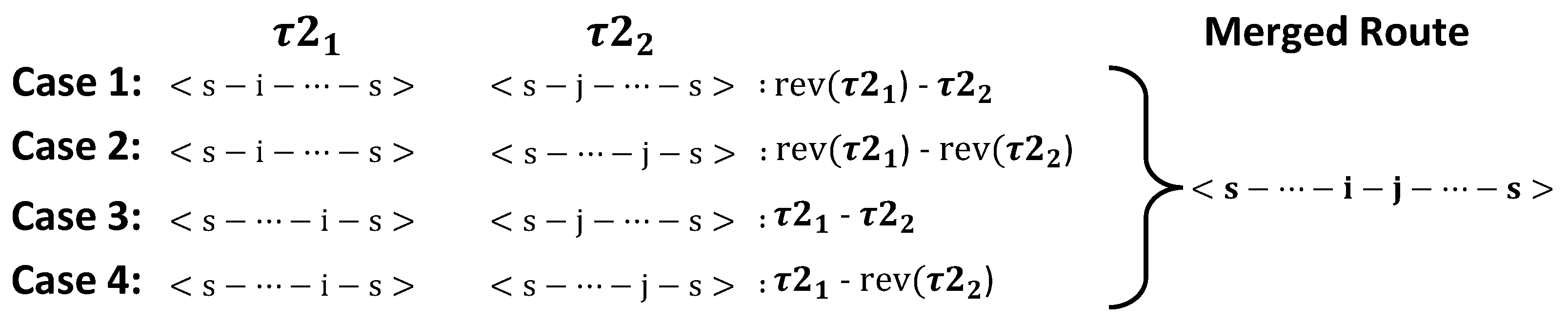
• At each iteration, the two routes that contain a pair of nodes $(i,j)$ with the highest savings value $s{2}_{ij}$ are selected from R (e.g., $\tau 2_1,\tau 2_2$). Then, the chosen routes are merged by connecting nodes i and j. All of the merging scenarios are graphically illustrated in Figure 3. Based on the way in which nodes i and j are connected to the respective satellite, one or both of the routes must be reversed in order to be able to connect nodes i and j. In this context, note that the reversed version of a tour $\tau 2_1$ is denoted by $\mathsf{rev}\left(\tau 2_1\right)$. If the merged route is infeasible in terms of vehicle capacity or time windows, the route is eliminated, and merging continues considering the pair of nodes with the next-highest savings value. If the merged route is battery infeasible, a charging station r with a lowest insertion cost is inserted between node i and j (e.g., $<\mathsf{s}-\dots -\mathsf{i}-\mathsf{r}-\mathsf{j}-\dots -\mathsf{s}>$). In these cases in which the route is still infeasible after charging station insertion, it is eliminated, and merging continues with the next pair of customers from the savings list. This procedure is repeated while the savings list is not empty. After merging, some of the charging stations that were previously added to the routes may become redundant. These charging stations are removed from the merged route.
• Update the savings list as described in step 2 and repeat step 3 until no further pairs of tours can be merged.
• Finally, the customers in $L_u$ (the list of unvisited customers) are inserted into the constructed tours using the greedy insertion operator, which is described in detail in Section 4.3.3.

Algorithm 1 Modified C&W Savings Heuristic for the 2E-EVRP-TW.

1: Assign customers to the nearest satellite 2: Determine the latest possible visiting time $\left(tw{l}_s\right)$ for each satellite $s\in N_S$ 3: Construct first echelon routes using the savings heuristic 4: for each satellite s do 5:    Create back-and-forth tours for each customer $i\in N_C^s$$(s-i-s)$ 6:    if the created tour is infeasible in terms of the battery constraints then 7:      Insert a charging station using the greedy CS insertion operator (see Section 4.3.3) 8:      if the tour is still infeasible then 9:         Discard the tour and add the customer to the unvisited customer list $L_u$ 10:      end if 11:    end if 12:    Generate the savings list and sort it in descending order based on the savings values 13:    while savings list is not empty do 14:      Merge the two tours with the greatest savings value 15:      if vehicle capacity or time window constraints are violated then 16:         Discard the tour and remove the corresponding pair of customers from the savings list 17:      else 18:         if the merged tour is infeasible in terms of the battery constraint then 19:           Insert a charging station with a minimum insertion cost 20:           if the tour is still infeasible then 21:              Discard the tour and remove the pair of customers from the savings list 22:           else 23:              Accept the merged tour and update the saving list 24:           end if 25:         else 26:           Accept the merged tour and update the saving list 27:         end if 28:      end if 29:    end while 30:    Insert all customers from $L_u$ into the constructed tours using the greedy customer insertion operator (see Section 4.3.3) 31: end for

Finally, note that the same procedure is applied to construct routes for the large vehicles in the first echelon. In this case, all aspects related to batteries and charing stations are removed from the heuristic procedure.

4.3. Variable Neighborhood Search for the 2E-EVRP-TW

The initial solution constructed by our version of the C&W savings heuristic from above is used as input for a variable neighborhood search (VNS) approach outlined in the following. VNS was proposed by [41] to solve complex combinatorial optimization problems. Unlike other algorithms based on local search, VNS uses multiple neighborhood structures and makes use of them during the search based on a set of pre-defined rules. This dynamic search mechanism allows the algorithm to intensify the search in the vicinity of good solutions, but also to diversify the search in order to avoid getting stuck in local optima. In particular, intensification is achieved by applying a local search procedure in order to reach locally optimal solutions, while shaking operators are used in order to diversify the search process and to explore different neighborhoods. For these reasons, the choice of appropriate neighborhood structures/operators for local search and for shaking is crucial. So far, VNS has shown state-of-the-art performance for a wide range of optimization problems, including the facility layout problem [42], scheduling problems [43,44,45], portfolio optimization [46,47], assembly and disassembly line balancing [48] and various routing problems [49,50,51,52].

Algorithm 2 presents a pseudo-code of our implementation of VNS for the 2E-EVRP-TW. The proposed algorithm starts by taking an initial solution $S_{init}$ as input. Then, the neighborhood structures used for shaking $N_k^{shake},(k=1,\dots ,k_{max})$ and the ones used for local search $N_h^{local},(h=1,\dots ,h_{max})$ are determined. These neighborhood structures will be explained in detail in following sections. However, note that, in addition to rather standard inter-route and intra-route operators, our VNS also makes use of so-called destroy-and-repair operators for the shaking step. Operators such as these ones were mostly introduced in the context of approaches based on large neighborhood search (and very large neighborhood search) algorithms and have shown to be highly useful for exploring large search spaces [53]. In particular, the reconstruction of a partially destroyed solution using various reinsertion operators has the potential to produce solutions that may have been difficult to reach otherwise. Concerning the specific case of VRP problems, removing rather large components of a solution and reinserting them into other positions of the solution may help reduce the number of routes and the number of vehicles, respectively.

After obtaining the initial solution $S_{init}$, both the current solution $S_{cur}$ and the best-so-far solution $S_{bsf}$ are initialized to $S_{init}$. At each main iteration of VNS, the shaking neighborhoods are randomly ordered. This order is then used until the current neighborhood utilized for shaking (indicated by k) is the $k_{max}$-th neighborhood. Next, a random solution $S_{shake}$ is chosen from the current shaking neighborhood k. In case this neighborhood is a removal/destroy operator, the partially destroyed solution must subsequently be repaired with an insertion operator; see lines 15–17 of Algorithm 2. After re-constructing the first echelon tours of $S_{shake}$ using our C&W savings algorithm (line 18), local search is applied to $S_{shake}$. For this purpose we applied the variable neighborhood descent (VND) method shown in Algorithm 3. In the VND phase, a set of local search operators are applied to $S_{shake}$ in a predefined and fixed order. In this context, note that after each application of a shaking and/or a local search operator, the first echelon routes must be reconstructed since satellite demands may have changed.

In a basic VNS, only improved solutions are accepted. However, in the context of problems with many unfeasible solutions, this may cause the algorithm to get stuck during the search process. Therefore, we have adopted the method introduced by [54] for the solution acceptance decisions (lines 20–29). Based on this method, while improved solutions are always accepted, non-improving solutions are accepted with a certain probability $p_{accept}$. At each iteration, function ClcAcceptanceProbability() calculates $p_{accept}$ as follows:

$$p_{accept}=\frac{e^{(-(f_{ext}\left(S_{local}\right)-f_{ext}\left(S_{cur}\right)))}}{T}$$

(51)

Here, $f_{ext}\left(S_{cur}\right)$ and $f_{ext}\left(S_{local}\right)$ are values of the extended fitness function of the current solution and of the solution after local search, respectively. Lastly, T refers to the actual temperature value. At the beginning, T is initialized to an initial temperature $T_{init}$ which is decreased by $t^{-}$ at each main iteration of VNS (see line 30). In this way, while a non-improving solution is more likely to be accepted early during the search, the probability of accepting non-improving solutions will decrease with a growing iteration number. However, in case no improved solution was found during $iter\_n{i}_{max}$ iterations, T is reset to $T_{init}$ in order to enhance diversification.

Algorithm 2 VNS for the 2E-EVRP-TW.

1: input: an initial solution $S_{init}$ 2: $S_{shake}:$ Solution obtained after shaking 3: $S_{local}:$ Local solution after VND 4: $S_{cur}:$ Current solution 5: $S_{bsf}:$ Best-so-far solution 6: $iter\_ni:$ The number of non-improving solutions 7: $iter\_n{i}_{max}:$ The maximum iteration limit for non-improving solutions 8: Determine set of neighborhood structures for shaking $\{N_k^{shake}\mid k=1,\dots ,k_{max}\}$ and local search $\{N_h^{local}\mid h=1,\dots ,h_{max}\}$ 9: $S_{cur},S_{bsf}\leftarrow S_{init}$ 10: while the computational time limit is not reached do 11:    Create $\pi$ of the shaking neighborhoods $N_k^{shake}$ 12:    Set $k\leftarrow 1$ 13:    while $k\le k_{max}$ do 14:      Apply shaking: Choose $S_{shake}$ from $N_{\pi \left(k\right)}^{shake}\left(S_{cur}\right)$, the $\pi \left(k\right)$th shaking neighborhood of $S_{cur}$ 15:      if $N_{\pi \left(k\right)}^{shake}$ is a removal/destroy operator then 16:         Repair $S_{shake}$ 17:      end if 18:      Re-construct first echelon tours using C&W savings algorithm 19:      Apply local search: $S_{local}\leftarrow \mathsf{VND}$ (Sshake) 20:      $p_{accept}\leftarrow \mathsf{ClcAcceptanceProbability}($fext(Scur), fext(Slocal), T) 21:      $\rho \leftarrow \mathsf{rand}\left(\right)$ 22:      if $f_{ext}\left(S_{local}\right)$ < $f_{ext}\left(S_{bsf}\right)$ then $S_{bsf}\leftarrow S_{local}$ 23:      if $f_{ext}\left(S_{local}\right)$ < $f_{ext}\left(S_{cur}\right)$ or $\rho <p_{accept}$ then 24:         $S_{cur}\leftarrow S_{local}$ 25:         $k\leftarrow 1$ 26:      else 27:         $k\leftarrow k+1$ 28:         $iter\_ni\leftarrow iter\_ni+1$ 29:      end if 30:      Decrease T by $t^{-}$ 31:      if $iter\_ni=iter\_n{i}_{max}$ then 32:         $T\leftarrow T_{init}$ 33:         $iter\_ni\leftarrow 0$ 34:      end if 35:    end while 36: end while

The following four sections will provide a detailed description of standard shaking operators, removal/destroy operators, repair operators, and local search neighborhoods, respectively.

4.3.1. Standard Shaking Operators

Random cyclic exchange: This operator was originally introduced by [55]. It transfers a node sequence (consisting of customers and/or charging stations) from one route to another in a cyclic way. This operator is quite advantageous for many sequence-based combinatorial optimization problems as it enables the generation of a large variety of moves with a single operator.

Algorithm 3 Variable Neighborhood Decent (VND).

1: input: $S_{shake}$ 2: $S_{VND}:$ Solution obtained after applying a local search operator 3: Set $h\leftarrow 1$ 4: while$h\le h_{max}$do 5:    Generate $S_{VND}$ from the hth local search neighborhood of $S_{shake}$$(S_{VND}:N_h^{local}\left(S_{shake}\right))$ 6:    if $f_{ext}\left(S_{VND}\right)$ < $f_{ext}\left(S_{shake}\right)$ then 7:      $S_{shake}\leftarrow S_{VND}$ 8:      $h\leftarrow 1$ 9:    else 10:      $h\leftarrow h+1$ 11:    end if 12: end while 13: output: $S_{shake}$

The cyclic exchange operator we have applied takes two parameters as input: (1) the number of routes ($\zeta$) to be involved in the cyclic move, and (2) the maximum number of nodes (${\theta }_{max}$) to be transferred from one route to another. First, the operator randomly selects $\zeta$ routes. Then, a random integer number $\theta$ from the interval [1, ${\theta }_{max}$] is independently determined for each route involved in the cyclic move. This value refers to the route-specific length of the node sequence to be transferred. Finally, $\theta$ consecutive nodes are randomly selected from each route and transferred to the next route in the cyclic move. If $\zeta$ is greater than the total number of routes existing in a solution, then $\zeta$ is set to the total number of routes. Similarly, if $\theta$ is greater than the total number of nodes in a route, then $\theta$ is readjusted. The optimal values for both parameters are determined by parameter tuning (see Section 5.2). Figure 4 illustrates a cyclic exchange move with three routes.

Random sequence relocation: This operator selects a node sequence from one route and transfers it to another route. The origin and destination routes, the node sequence to be relocated, and the insertion position in the destination route are determined randomly. Parameter $ma{x}_n$ limits the number of nodes to be transferred. The optimal value for $ma{x}_n$ is determined by parameter tuning (Section 5.2).

4.3.2. Removal/Destroy Operators

One of the most critical aspects of a destroy operators is deciding on the number of nodes in the solution to be removed. Limiting the amount of destruction too much may cause a poor exploration performance of the algorithm. On the contrary, repairing a largely destroyed solution can be time-consuming and may result in a poor quality solution depending on the utilized repair procedure [53]. Therefore, we used a random removal rate between a lower and an upper bound to determine how many nodes (or routes) will be removed from the current solution. Well-working upper and lower bounds are decided via parameter tuning (Section 5.2) and fixed for each group of instances.

Random customer removal: First, a random number $\rho$ is drawn from the interval $[rr{1}_{Lb},rr{1}_{Ub}]$. This number is the fraction of customers to be removed from the solution, henceforth called the removal rate. Note that $rr{1}_{Lb}$ and $rr{1}_{Ub}$ are the lower and upper bounds for the removal rate. Finally, a randomly chosen number of max{1, $\lfloor \rho \ast n_c\rfloor$ } randomly chosen customers are removed from the current solution and added to a removal list $L_r$.

Random route removal: Similar to the random customer removal operator above, a random number $\rho$ is drawn from the interval $[rr{2}_{Lb},rr{2}_{Ub}]$. This number is the fraction of routes to be removed from the solution. Assume that solution S has n routes in the second echelon. After drawing number $\rho$, a number of max{1, $\lfloor \rho \ast n\rfloor$ } randomly chosen routes are removed from the current solution and all customers from these routes are added to a removal list $L_r$.

Close satellite: This operator closes a randomly chosen satellite and adds all the customers served through this satellite to a removal list $L_r$.

4.3.3. Repair Operators

A partially destroyed solution may either be repaired using an exact or a heuristic approach. Although exact approaches guarantee the optimal insertion of removed customers or routes, they are much more time consuming than heuristic approaches, especially when a rather large part of the solution is destroyed. Moreover, too much optimality in the repair operator may limit the diversification capabilities of the search. Therefore, we have applied greedy and best-insertion strategies for repairing partially destroyed solutions; see also [56,57]. In the following, partially destroyed solutions are labelled $S_d$.

Greedy customer insertion: This operator reinserts each customer from $L_r$ into the partially destroyed solution $S_d$ according to the last-in-first-out (LIFO) principle. Henceforth, $N_{S_d}$ denotes the set of nodes (customers and charging stations) that still form part of the partially destroyed solution $S_d$. Let $v\in L_r$ be the customer that is to be re-inserted into $S_d$. First, for each pair $i,j\in N_{S_d}$ such that i and j are consecutive nodes in one of the routes of $S_d$, the insertion cost ${\delta }_{vij}$ is calculated as follows:

$${\delta }_{vij}=d{2}_{iv}+d{2}_{vj}-d{2}_{ij}$$

(52)

Then, customer v is inserted at the position with the lowest insertion cost. Suppose that the obtained route after insertion is infeasible in terms of vehicle capacity or time windows constraints. In this case, customer v is inserted at the next-cheapest position in terms of the insertion cost, and so on. If no feasible insertion position can be found, the customer is finally inserted at the initially best position, ignoring the infeasibility. In case of battery infeasibility, a charging station is added to the route. These procedures are applied until no customer remains in $L_r$.

Greedy customer insertion with noise: This operator is a special version of the greedy customer insertion operator described above. It utilizes the following modified cost function with a noise parameter for calculating the insertion cost of a customer v:

$$\begin{array}{c}\hfill {\delta }_{vij}^{noise}={\delta }_{vij}+d_{max}+\alpha +\beta \end{array}$$

(53)

Here, $d_{max}$ refers to the maximum distance between all nodes in $N_{SRC}$, and $\alpha$ refers to the noise parameter set to 0.1 [57,58,59,60]. Finally, $\beta$ is a uniform random number generated independently for the calculation of each cost value from the interval $[-1,1]$.

Best customer insertion: Instead of re-inserting customers from $L_r$ in the LIFO order, this operator aims to find the best insertion position for all customers. Each time, the insertion costs of all remaining customers from $L_r$ are calculated using Equation (52). Then, the customer with the best insertion cost is inserted into the best possible position. This operator is much more time consuming than the greedy customer insertion operator. It may, however, lead to better results. Infeasible insertions are handled in the same way as the greedy customer insertion operator.

Greedy CS insertion: In the case of battery infeasibility, this operator inserts a charging station with the lowest insertion cost at the point at which infeasibility occurs. Figure 5 illustrates the insertion of a charging station to a battery-infeasible route. Assuming that the electric vehicle runs out of battery before reaching node $v_4$, the operator first tries to insert a charging station $r^{\ast }:=\mathrm{argmax}\{d{2}_{3r}+d{2}_{r4}-d{2}_{34}\mid r\in N_R\}$ between nodes $v_3$ and $v_4$. In case the battery level is not high enough to reach the charging station that is to be inserted, a possible insertion is tried before node $v_3$, etc.

4.3.4. Local Search Neighborhoods

For the local search phase (that is, for the application within VND), the algorithm makes use of three inter-route operators (exchange(1,1), shift(1,0), and swap) and three intra-route operators (relocation, two_opt, and CS_reinsertion). In all these neighborhoods—except for CS_reinsertion—we use the first-improvement strategy, that is, a neighborhood exploration stops once the first improving solution is found. Infeasible moves are also allowed but they are penalized. Figure 6 graphically illustrates these local search neighborhoods.

The exchange(1,1) neighborhood considers all exchanges of each customer with every other customer not in the same route. The shift(1,0) neighborhood looks at all possibilities of removing a customer from its current route and inserting it at any position in the rest of the routes. Next, the relocation operator removes each customer from its current position and inserts it into another position in the same route. The swap neighborhood considers changing the positions of two selected nodes of the same route. The two_opt neighborhood considers all possibilities of selecting two non-consecutive nodes in the same route and reversing the node sequence between the two selected nodes. Note that there must be at least three nodes between the two selected nodes in order not to repeat moves already considered in the swap operator. The CS_relocation operator removes the current charging stations of a route and reinserts them in different positions in the same route in order to find the best positions for the charging stations. Unlike CS_relocation, the CS_reinsertion operator removes the current charging stations from a route. Instead of reinserting the removed ones, the greedy charging station insertion operator from the previous section is applied to repair the route. Thus, charging stations different from the removed ones may be inserted into the route.

5. Computational Experiments

In addition to our C&W savings heuristic and VNS we also tried to solve all problem instances with the MILP solver CPLEX. All experiments were performed on a cluster of machines with Intel Xeon CPU 5670 CPUs with 12 cores of 2.933 GHz and a minimum of 32 GB RAM. Note that CPLEX version 12.10 was used in one-threaded mode.

5.1. Generation of 2E-EVRP-TW Instances

Due to a lack of available benchmark sets for the 2E-EVRP-TW, we generated new problem-specific instance sets by extending the benchmark sets provided in [12]. These instances were proposed for the electric vehicle routing problem with time windows and consist of 36 small and 56 large instances. Small instances are composed of 5, 10, or 15 customers with a varying number of charging stations (between 2 and 5), while the large ones include 100 customers and 21 charging stations. We have extended these instance sets following the methodology proposed in [26]. In particular, first, the number of satellites to be added to each instance was determined. Then, the locations of those satellites and the one of a single central warehouse was specified.

Concerning the number of satellites, we decided to use one single satellite in the case of small instances with at most 10 customers, two satellites in the case of 15 customers, and eight satellites for the large instances. Note that the customers of each instance are scattered over the intersections of a 100 × 100 grid. The location of the single central warehouse was determined for each instance to be outside this area, at $(50,150)$. The single satellite in the case of instances with at most 10 customers was placed at $(50,75)$, while the two satellites in the case of instances with 15 customers were places at $(50,25)$ and $(50,75)$. Finally, the eight satellites for all remaining instances were placed at $(25,25)$, $(25,50)$, $(25,75)$, $(50,25)$, $(50,75)$, $(75,25)$, $(75,50)$ and $(75,75)$. Figure 7 shows examples of all three cases.

In addition, we updated the customers’ time windows by adding the distance between the location of the central warehouse in the original instance set and the new central warehouse as an offset value. Lastly, we modified the capacities of the electric vehicles and large trucks, considering the fact that instances labeled with C2, R2, and RC2 are more capacity constrained as compared to those labeled C1, R1, and RC1. In particular, we have fixed the capacity ratio between large trucks and electric vehicles to $4/0.5$ for instances of the first type, and to $2/0.25$ for instances of the second type. All benchmark instances generated in this study and the executable of the proposed algorithm are available at https://github.com/manilakbay/2E-EVRP-TW, accessed on 12 January 2022.

5.2. Parameter Tuning

In order to determine well-working parameter values for our algorithms we have utilized the scientific tuning software irace [61].

Table 1. Parameters of our C&W savings heuristic together with their domains.

Parameter	Description	Domain
$\lambda$	Route redesign parameter	$\{0.0,0.1,\dots ,0.9,1.0\}$
$\mu$	Asymmetry of information	$\{0.0,0.1,\dots ,0.9,1.0\}$
$\gamma$	Assignment priority	$\{1.0,1.1,\dots ,1.9,2.0\}$

and 

Table 2. VNS parameters and their domains.

Parameter	Description	Domain
$rr{1}_{Lb},rr{1}_{Ub}$	Customer removal rate and lower and upper bounds	$\{0.0,0.1,\dots ,0.9,1.0\}$
$rr{2}_{Lb},rr{2}_{Ub}$	Route removal rate and lower and upper bounds	$\{0.0,0.1,\dots ,0.9,1.0\}$
$p_{init}$	Initial penalty value	$\{10,15,20\}$
$p_{min}$	Minimum penalty value	$\{0.5,1,3,5\}$
$p_{max}$	Maximum penalty value	$\{25,30,35,40\}$
$p_{iter}$	Iteration count parameter for penalty procedure	$\{1,2,3\}$
$p^{+}$	Augmentation parameter for penalty	$\{3,5,7,9\}$
$p^{-}$	Reduction parameter for penalty	$\{1.0,1.1,\dots ,1.9,2.0\}$
$T^{init}$	Initial temperature	$\{50,100,150,200\}$
$t^{-}$	Update parameter for the temperature	$\{1.0,1.1,\dots ,1.9,2.0\}$
$iter\_n{i}_{max}$	Maximum number of non-improving iterations	$\{100,200,500,1000,10,000\}$
$\zeta$	The number routes involved in a cyclic exchange	$\{1,2,3,4\}$
${\theta }_{max}$	The maximum number of nodes to be transferred (cyclic exchange)	$\{1,2,3,4\}$

summarize the parameters that are subject to tuning for our C&W savings heuristic and for the VNS together with the considered value domains.

Due to large differences in instance size, we decided to tune our VNS algorithm (including the parameters of the C&W savings heuristic) separately for small and for large problem instances. In the first case (small instances), instances C101_C10, R102_C10, RC102_C10, C103_C15, R102_C15 and RC103_C15 were used for tuning. In the case of the large instances, instances C101_21, C201_21, R101_21, R201_21, RC101_21 and RC201_21 were used. For each of the two tuning runs, the budget of irace was fixed to 2000 algorithm runs. In the context of small instances, the computation time limit of each run was fixed to 150 CPU seconds, while it was fixed to 900 CPU seconds in the case of the large problem instances.

Table 3. Parameter values determined by irace for the C&W savings heuristic.

Parameters	Small Instances	Large Instances
$\lambda$	1.3	1.1
$\mu$	0.3	0.1
$\gamma$	0.9	0.6

and 

Table 4. Parameter values determined by irace for VNS.

Parameters	Small Instances	Large Instances
$rr{1}_{Lb}$	0.1	0.3
$rr{1}_{Ub}$	0.7	0.4
$rr{2}_{Lb}$	0.1	0.4
$rr{2}_{Ub}$	0.6	0.4
$p_{init}$	15	20
$p_{min}$	5	0.5
$p_{max}$	40	35
$p_{iter}$	1	2
$p^{+}$	9	5
$p^{-}$	1.6	1.4
$t^{init}$	200	100
$t^{-}$	1.3	2
$iter\_n{i}_{max}$	1000	100
$\zeta$	2	4
${\theta }_{max}$	4	2

show the obtained parameter value settings for the two cases. It is worth noting, for example, that well-working ranges for the removal rates (in the context of the removal/destroy operators) are considerably smaller in the case of the large instances when compared to those for small instances. One reason for this may be that repairing a largely destroyed solution is time consuming and may lead to a rather bad quality solution. On the other hand, a high removal rate may be considered as a perturbation mechanism that helps to escape from local minima in the context of small instances.

5.3. Numerical Results

In the following we provide a detailed comparison of the following methods. First, we applied both CPLEX (version 12.10) and our C&W savings heuristic to all problem instances. Hereby, CPLEX was given a time limit of 2 h of CPU time for each problem instance. Next we also applied two versions of VNS. The full version of VNS is henceforth denoted by VNS${}_{\mathrm{full}}$. In contrast, VNS${}_{\mathrm{red}}$ is a reduced version of VNS that only utilizes classical inter-route and intra-route shaking operators. A comparison of these two variants is interesting, because it shows how much the destroy and repair operators add to the performance of VNS. Note that both versions of VNS were applied with a computation time limit of 150 CPU seconds in the case of small problem instances, and 900 CPU seconds for large problem instances. Moreover, both versions of VNS were applied 10 times to each problem instance.

Table 5. Computational results for small-sized instances with 5 customers.

Instances			CPLEX					C&W Savings Heuristic				VNS${}_{\mathbf{red}}$					VNS${}_{\mathbf{full}}$
Name	${\mathit{nv}}_1$	${\mathit{nv}}_2$	m	n	Dist	Gap(%)	$\overline{\mathit{t}\left(\mathit{s}\right)}$	m	n	Dist	$\overline{\mathit{t}\left(\mathit{s}\right)}$	m	n	Dist	Avg	$\overline{\mathit{t}\left(\mathit{s}\right)}$	m	n	Dist	Avg	$\overline{\mathit{t}\left(\mathit{s}\right)}$
C101_C5	1	2	1	2	385.49	0	1.67	1	3	442.19	0.00021	1	2	385.49	385.49	0.989	1	3	385.49	385.49	12.509
C103_C5	1	1	1	1	341.33	0	0.09	1	2	360.94	0.00011	1	1	341.33	341.33	0.006	1	1	341.33	341.33	0.502
C206_C5	1	1	1	1	417.31	0	5.97	1	3	480.9	0.00017	1	1	417.31	417.31	0.001	1	1	417.31	417.31	0.001
C208_C5	1	1	1	1	381.91	0	0.31	1	1	383.07	0.00011	1	1	381.91	381.91	0.001	1	1	381.91	381.91	0.001
R104_C5	1	2	1	2	317.02	0	1.61	1	1	317.78	0.00012	1	1	317.02	317.02	0.001	1	1	317.02	317.02	0.001
R105_C5	1	3	1	2	453.74	0	9.57	1	1	677.61	0.00014	1	2	453.74	495.16	0.000	1	2	453.74	453.74	29.693
R202_C5	1	1	1	1	347.82	0	0.21	1	1	348.29	0.00010	1	1	347.82	347.82	0.001	1	1	347.82	347.82	0.001
R203_C5	1	1	1	1	371.31	0	0.21	1	1	387.92	0.00016	1	1	386.48	386.48	0.001	1	1	371.31	371.31	7.203
RC105_C5	1	3	1	3	432.64	0	28.84	1	3	496.72	0.00015	1	2	432.64	435.77	0.404	1	2	432.64	437.34	21.488
RC108_C5	1	2	1	2	460.89	0	24.24	1	2	702.23	0.00016	1	2	460.89	460.89	0.008	1	2	460.89	460.89	3.281
RC204_C5	1	1	1	1	332.86	0	0.64	1	1	649.44	0.00015	1	1	332.86	332.86	0.018	1	1	332.86	332.86	0.015
RC208_C5	1	1	1	1	327.30	0	0.37	1	1	331.77	0.00010	1	1	331.77	331.77	0.000	1	1	327.30	327.30	15.193
average			-	-	380.80	-	6.15	-	-	464.905	0.00014	-	-	382.44	386.15	0.119	-	-	380.80	381.19	7.491

,

Table 6. Computational results for small-sized instances with 10 customers.

Instances			CPLEX					C&W Savings Heuristic				VNS${}_{\mathbf{red}}$					VNS${}_{\mathbf{full}}$
Name	${\mathit{nv}}_1$	${\mathit{nv}}_2$	m	n	Dist	Gap(%)	$\overline{\mathit{t}\left(\mathit{s}\right)}$	m	n	Dist	$\overline{\mathit{t}\left(\mathit{s}\right)}$	m	n	Dist	Avg	$\overline{\mathit{t}\left(\mathit{s}\right)}$	m	n	Dist	Avg	$\overline{\mathit{t}\left(\mathit{s}\right)}$
C101_C10	1	4	1	4	538.31	0	3021.74	1	5	568.85	0.00017	1	3	538.31	538.74	0.568	1	4	538.31	538.31	13.233
C104_C10	1	3	1	2	484.32	0	5309.78	1	4	663.74	0.00024	1	2	484.32	484.32	0.979	1	2	484.32	484.32	7.119
C202_C10	1	3	1	2	425.53	0	152.011	1	5	625.02	0.00021	1	2	425.53	425.53	0.030	1	2	425.53	425.53	2.018
C205_C10	1	3	1	3	415.48	0	157.97	1	3	435.37	0.00024	1	2	415.48	419.64	0.005	1	3	415.48	415.48	1.006
R102_C10	1	4	1	3	505.50	0	6150.84	1	4	648.65	0.00019	1	3	505.50	505.50	2.477	1	3	505.50	524.59	22.556
R103_C10	1	3	1	2	436.08	9.27	6318.99	1	3	613.76	0.00024	1	2	436.08	436.08	2.396	1	2	436.08	437.51	3.600
R201_C10	1	2	1	2	460.71	0	2686.75	1	4	730.95	0.00017	1	2	460.71	460.71	2.838	1	2	460.71	460.71	16.455
R203_C10	1	2	1	1	436.51	0	2192.71	1	1	437.75	0.00021	1	1	436.51	436.51	0.002	1	1	436.51	436.51	0.002
RC102_C10	1	5	1	4	618.75	16.85	7079.09	1	5	684.93	0.00026	1	4	618.75	618.75	41.620	1	4	618.75	618.75	11.025
RC108_C10	1	4	1	4	637.23	24.28	6739.84	1	4	721.2	0.00020	1	3	559.88	559.88	0.097	1	3	559.88	559.88	0.016
RC201_C10	1	4	1	3	495.54	0	969.86	1	4	634.13	0.00021	1	2	495.54	497.04	0.004	1	3	495.54	495.54	2.528
RC205_C10	1	3	1	3	576.17	0	462.62	1	3	702.34	0.00025	1	2	576.17	577.76	0.130	1	3	576.17	576.17	15.366
average			-	-	502.51	-	3436.85	-	-	622.22	0.00022	-	-	496.06	496.70	4.262	-	-	496.06	497.77	7.910

and

Table 7. Computational results for small-sized instances with 15 customers.

Instances			CPLEX					C&W Savings Heuristic				VNS${}_{\mathbf{red}}$					VNS${}_{\mathbf{full}}$
Name	${\mathit{nv}}_1$	${\mathit{nv}}_2$	m	n	Dist	Gap(%)	$\overline{\mathit{t}\left(\mathit{s}\right)}$	m	n	Dist	$\overline{\mathit{t}\left(\mathit{s}\right)}$	m	n	Dist	Avg	$\overline{\mathit{t}\left(\mathit{s}\right)}$	m	n	Dist	Avg	$\overline{\mathit{t}\left(\mathit{s}\right)}$
C103_C15	1	5	-	-	-	-	-	1	6	690.99	0.00036	1	3	575.18	582.02	4.925	1	4	575.18	575.18	0.623
C106_C15	1	4	1	3	500.32	13.37	7182.91	1	6	681.31	0.00022	1	3	516.60	524.10	2.100	1	3	516.60	516.60	1.027
C202_C15	1	5	1	4	714.81	32.23	7183.04	1	6	729.87	0.00034	1	4	617.24	618.66	29.966	1	3	550.32	550.32	12.454
C208_C15	1	3	1	2	550.02	15.56	7182.95	1	4	737.61	0.00023	1	2	619.73	619.73	6.976	1	2	550.02	550.02	22.000
R102_C15	1	7	-	-	-	-	-	1	9	950.25	0.00026	1	5	716.56	716.56	9.523	1	5	716.56	716.56	12.056
R105_C15	1	5	-	-	-	-	-	1	8	777.77	0.00038	1	4	607.96	607.96	30.850	1	4	607.96	607.96	25.605
R202_C15	1	3	1	3	719.61	35.36	7198.17	1	6	990.37	0.00043	1	2	593.69	597.79	8.033	1	3	593.69	593.69	60.988
R209_C15	1	3	1	2	475.10	10.09	7182.43	1	5	711.09	0.00024	1	2	475.10	519.46	0.712	1	1	475.10	482.30	77.386
RC103_C15	1	5	-	-	-	-	-	1	7	745.82	0.00035	1	4	616.32	622.10	1.565	1	5	616.32	616.32	1.803
RC108_C15	1	5	-	-	-	-	-	1	7	716.22	0.00026	1	5	603.87	603.87	0.214	1	5	603.87	615.11	0.033
RC202_C15	1	3	1	3	552.70	16.06	7182.65	1	5	697.24	0.00033	1	3	601.86	601.86	2.395	1	2	552.70	587.11	11.600
RC204_C15	1	3	1	2	485.34	13.93	7183.03	1	3	604.05	0.00035	1	2	551.56	551.56	0.670	1	2	485.34	485.34	15.566
average			-	-	-	-	-	-	-	752.72	0.00031	-	-	591.31	597.14	8.161	-	-	570.30	574.71	20.095

show the numerical results for small problem instances with 5, 10, and 15 customers, respectively. The structure of these tables is as follows. Instance names are given in the first column, and the maximum number of vehicles in the first and second echelons are provided in the second and third columns, respectively. These numbers are only necessary for the application of CPLEX. After the first three table columns, there are four blocks of columns, presenting the results of our four approaches. The first three columns of each block (with headings ‘n’, ‘m’, and ‘dist’) are the same for all four approaches. Hereby, columns ‘n’ and ‘m’ provide the number vehicles utilized by the respective solutions in the first echelon and the second echelon, respectively. In the case of VNS${}_{\mathrm{full}}$ and VNS${}_{\mathrm{red}}$  these numbers refer to the best solution found within 10 independent runs. Column ‘dist’ provides the objective function values of the solutions generated by the four approaches. In the case of VNS${}_{\mathrm{full}}$ and VNS${}_{\mathrm{red}}$, ‘dist’ shows the objective function value of the best solution found in 10 runs, while an additional column with the heading ‘avg’ provides the average objective function value of the best solutions of each of the 10 runs. Next, columns with heading ‘$\overline{t\left(s\right)}$’ show the computation time of CPLEX, our C&W savings heuristic and the average computation times of VNS${}_{\mathrm{full}}$ and VNS${}_{\mathrm{red}}$ to find the best solutions in each run. Finally, column ‘gap(%)’ provides the gap (in percent) between the best solution and the best lower bound found by CPLEX. Note that, in the case where the gap value is zero, CPLEX has found an optimal solution.

The following observations can be made: First, apart from instances R103_C10, RC102_C10, and RC108_C10, CPLEX was able to solve the mathematical model—within 2 h of CPU time—for all instances with five and ten customers to optimality. For two of the remaining three cases, CPLEX was able to provide feasible solutions of the same quality as VNS${}_{\mathrm{full}}$ and VNS${}_{\mathrm{red}}$, without being able to prove optimality. However, for the instances with 15 customers, the performance of CPLEX heavily starts to degrade. The reason for the rapidly decreasing performance of CPLEX is that the size and complexity of the MILP model sharply increase based on the instance size. For instance, the average number of variables and constraints of the MILP model for the instances containing five customers is 986 and 2235, respectively. These values increase to 4008 and 9363 for the instances with 10 customers and to 13,125 and 31,482 for the instances with 15 customers. In this latter case, CPLEX could only provide valid solutions (without being able to prove optimality) in seven out of 12 instances. Nevertheless, for one instance (C106_15), CPLEX produced a better solution than both VNS variants.

Both VNS variants performed comparably on small problem instances with 5 and 10 customers. They were able to find solutions with the same objective function values as those of CPLEX. However, the performance of the two VNS variants starts to differ on the instances with 15 customers. While VNS${}_{\mathrm{full}}$ provides results at least as good as CPLEX for all instances except for C106_C15, VNS${}_{\mathrm{red}}$ only does so in seven out of 12 cases. Considering those instances for which CPLEX was able to obtain a solution, both VNS variants improved the solution quality of CPLEX, on average, by 0.55% (VNS${}_{\mathrm{red}}$) and 6.86% (VNS${}_{\mathrm{full}}$ ). In fact, VNS${}_{\mathrm{full}}$ outperforms VNS${}_{\mathrm{red}}$ both in terms of best-performance (column ‘dist’) and in terms of average-performance (column ‘avg’). Note also that the running times of both VNS${}_{\mathrm{full}}$ and VNS${}_{\mathrm{red}}$ are in the order of seconds. While the superiority of both VNS${}_{\mathrm{full}}$ and VNS${}_{\mathrm{red}}$ over CPLEX in terms of CPU time is more significant for the instances with 10 and 15 customers, see Table 6 and Table 7, only VNS${}_{\mathrm{red}}$ provides better CPU times for the instances with 5 customers. Finally, note that the results of the C&W savings heuristic are, in the context of these small problem instances, approx. 20% worse than the best results obtained. This is, however, achieved in very low computation times of a fraction of a second, which shows that our C&W savings heuristic is a good candidate for producing the initial solutions of VNS.

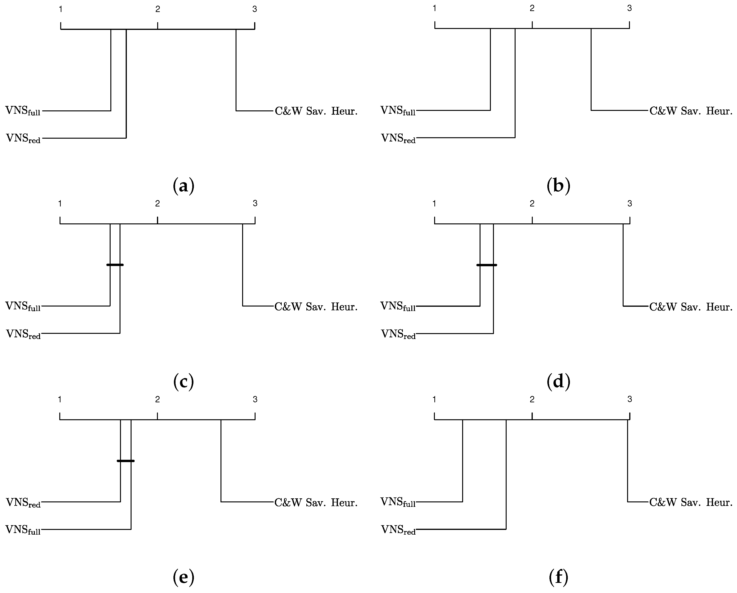
Next, we analyze the results of the four approaches when applied to the large problem instances of our benchmark set. These results are shown in

Table 8. Computational results for large-sized clustered instances.

Instances			C&W Savings Heuristic				VNS${}_{\mathbf{red}}$						VNS${}_{\mathbf{full}}$
Name	${\mathit{n}}_{\mathit{k}}$	${\mathit{n}}_{\mathit{v}}$	m	n	Dist	$\overline{\mathit{t}\left(\mathit{s}\right)}$	m	n	Dist	Avg	Imp(%)	$\overline{\mathit{t}\left(\mathit{s}\right)}$	m	n	Dist	Avg	Imp(%)	$\overline{\mathit{t}\left(\mathit{s}\right)}$
C101_C21	3	25	3	39	1941.16	0.005	3	20	1513.91	1562.77	19.49	499.70	3	20	1494.18	1538.74	20.73	579.98
C102_C21	3	28	3	33	1822.02	0.005	3	21	1501.66	1506.95	17.29	537.57	3	19	1447.86	1487.11	18.38	572.03
C103_C21	3	26	3	29	1702.89	0.005	3	20	1447.98	1463.34	14.07	509.37	3	19	1399.25	1425.80	16.27	656.63
C104_C21	3	31	3	24	1580.07	0.005	3	20	1435.04	1446.17	8.47	405.19	3	19	1400.52	1439.76	8.88	540.97
C105_C21	4	43	3	36	1877.85	0.005	3	20	1522.97	1541.60	17.91	359.00	3	20	1493.69	1521.13	19.00	466.13
C106_C21	4	37	3	35	1791.74	0.004	3	20	1474.74	1491.70	16.75	361.26	3	20	1429.75	1476.85	17.57	536.93
C107_C21	4	41	3	34	1838.83	0.005	3	20	1499.81	1513.36	17.70	400.85	3	20	1485.7	1513.18	17.71	582.44
C108_C21	3	33	3	29	1687.15	0.005	3	20	1461.25	1476.72	12.47	483.00	3	20	1450.96	1489.63	11.71	523.87
C109_C21	4	31	3	26	1619.19	0.005	3	20	1447.36	1456.90	10.02	326.59	3	20	1409.97	1455.93	10.08	673.76
C201_C21	3	20	2	35	1794.83	0.004	2	11	1251.62	1276.42	28.88	422.74	2	12	1208.76	1233.87	31.25	545.02
C202_C21	4	20	2	31	1672.52	0.005	2	12	1228.61	1260.08	24.66	532.72	2	12	1187.87	1232.74	26.29	703.08
C203_C21	3	19	2	27	1554.96	0.005	2	12	1197.45	1223.16	21.34	356.27	2	11	1201.4	1216.36	21.78	767.58
C204_C21	4	18	2	22	1411.07	0.005	2	12	1178.14	1191.92	15.53	464.31	2	11	1161.07	1181.40	16.28	577.96
C205_C21	4	20	2	21	1470.73	0.005	2	12	1226.48	1249.59	15.04	460.15	2	12	1205.23	1223.94	16.78	664.39
C206_C21	3	19	2	19	1399.11	0.005	2	12	1202.52	1222.94	12.59	519.78	2	11	1182.63	1198.54	14.34	556.03
C207_C21	3	19	2	20	1406.55	0.005	2	12	1195.1	1211.55	13.86	262.84	2	11	1173.7	1188.92	15.47	562.88
C208_C21	3	17	2	19	1393.28	0.005	2	12	1193.01	1221.40	12.34	429.15	2	11	1169.69	1188.85	14.67	652.98
average					1644.94	0.005			1351.63	1371.56	16.38	431.21			1323.66	1353.69	17.48	597.80

,

Table 9. Computational results for large-sized random instances.

Instances			C&W Savings Heuristic				VNS${}_{\mathbf{red}}$						VNS${}_{\mathbf{full}}$
Name	${\mathit{n}}_{\mathit{k}}$	${\mathit{n}}_{\mathit{v}}$	m	n	Dist	$\overline{\mathit{t}\left(\mathit{s}\right)}$	m	n	Dist	Avg	Imp(%)	$\overline{\mathit{t}\left(\mathit{s}\right)}$	m	n	Dist	Avg	Imp(%)	$\overline{\mathit{t}\left(\mathit{s}\right)}$
R101_C21	4	34	4	46	2546.45	0.006	4	25	2164.26	2187.39	14.10	573.91	4	26	2179.75	2306.91	9.41	589.70
R102_C21	3	32	4	37	2365.85	0.006	3	21	1840.45	1894.10	19.94	583.85	3	24	1843.45	2025.31	14.39	300.08
R103_C21	3	23	3	32	1974.87	0.006	3	19	1696.36	1754.36	11.17	657.28	3	19	1729.91	1829.33	7.37	350.64
R104_C21	2	20	3	23	1784.94	0.006	2	17	1473.50	1641.42	8.04	770.40	2	17	1470.20	1628.00	8.79	535.30
R105_C21	3	25	3	39	2216.4	0.005	3	23	1842.34	1898.80	14.33	539.41	3	22	1909.13	1975.78	10.86	463.62
R106_C21	3	28	3	32	2055.43	0.006	3	20	1737.88	1870.36	9.00	345.95	3	21	1723.88	1887.34	8.18	153.16
R107_C21	2	23	2	30	1725.89	0.007	2	18	1518.95	1671.82	3.13	287.01	2	18	1490.01	1670.00	3.24	323.49
R108_C21	2	21	2	23	1603.11	0.006	2	18	1454.99	1553.47	3.10	322.44	2	18	1449.13	1569.62	2.09	184.32
R109_C21	2	24	3	29	1947.31	0.006	2	18	1547.52	1694.54	12.98	356.45	2	19	1529.71	1683.81	13.53	386.16
R110_C21	2	23	2	26	1650.24	0.006	2	17	1451.04	1486.15	9.94	597.54	2	17	1470.57	1513.50	8.29	660.80
R111_C21	2	24	3	26	1805.69	0.006	2	18	1487.83	1572.49	12.91	579.21	2	17	1522.49	1593.35	11.76	483.22
R112_C21	2	23	2	20	1460.99	0.006	2	20	1457.06	1457.06	0.27	0.00	2	17	1413.86	1452.74	0.56	64.47
R201_C21	1	14	2	34	1912.59	0.006	1	12	1238.92	1265.99	33.81	486.39	1	9	1218.88	1252.17	34.53	639.80
R202_C21	1	12	2	29	1760.69	0.006	1	9	1158.64	1170.28	33.53	626.39	1	9	1135.84	1166.67	33.74	564.04
R203_C21	1	14	2	22	1587.76	0.007	1	8	1064.16	1093.38	31.14	513.09	1	7	1067.89	1096.69	30.93	542.58
R204_C21	1	9	2	17	1408.95	0.006	1	7	962.16	994.44	29.42	534.08	1	6	965.62	977.19	30.64	591.03
R205_C21	1	14	1	27	1522.45	0.006	1	9	1136.47	1167.99	23.28	711.65	1	7	1134.35	1155.14	24.13	452.03
R206_C21	1	12	1	23	1445.78	0.006	1	8	1106.23	1137.05	21.35	789.19	1	7	1092.55	1117.88	22.68	512.81
R207_C21	1	13	1	17	1334.95	0.006	1	7	1034.45	1072.21	19.68	588.03	1	7	1025.08	1055.93	20.90	512.99
R208_C21	1	12	1	16	1232.96	0.006	1	7	991.25	1018.02	17.43	484.88	1	7	970.31	996.20	19.20	519.00
R209_C21	1	15	1	23	1400.02	0.006	1	8	1078.55	1106.82	20.94	597.86	1	7	1078.00	1089.28	22.20	597.67
R210_C21	1	12	1	19	1350.21	0.006	1	8	1059.31	1090.53	19.23	515.34	1	7	1045.64	1068.65	20.85	480.40
R211_C21	1	9	1	18	1291.64	0.006	1	7	1030.77	1053.79	18.41	524.60	1	6	999.26	1034.15	19.93	421.96
average					1712.40	0.006			1371.00	1428.37	16.83	521.08			1368.07	1441.11	16.44	449.10

and

Table 10. Computational results for large-sized random-clustered instances.

Instances			C&W Savings Heuristic				VNS${}_{\mathbf{red}}$						VNS${}_{\mathbf{full}}$
Name	${\mathit{n}}_{\mathit{k}}$	${\mathit{n}}_{\mathit{v}}$	m	n	Dist	$\overline{\mathit{t}\left(\mathit{s}\right)}$	m	n	Dist	Avg	Imp(%)	$\overline{\mathit{t}\left(\mathit{s}\right)}$	m	n	Dist	Avg	Imp(%)	$\overline{\mathit{t}\left(\mathit{s}\right)}$
RC101_C21	3	28	4	38	2467.62	0.004	4	23	2044.99	2274.23	7.84	294.29	3	22	1907.52	2106.42	14.64	605.26
RC102_C21	3	29	4	36	2385.73	0.005	4	22	2004.78	2035.60	14.68	516.43	3	21	1834.97	2047.79	14.16	397.12
RC103_C21	3	28	4	29	2189.24	0.004	3	20	1747.98	1933.49	11.68	393.23	3	20	1728.17	1846.23	15.67	470.22
RC104_C21	2	26	2	26	1710.42	0.004	2	19	1644.36	1686.88	1.38	322.00	2	19	1645.35	1688.65	1.27	372.96
RC105_C21	3	23	5	33	2482.3	0.005	3	20	1789.64	1821.53	26.62	471.32	3	20	1802.85	1936.87	21.97	506.77
RC106_C21	3	23	3	33	2142.63	0.005	3	20	1760.23	1797.62	16.10	584.16	3	19	1750.61	1807.42	15.64	450.61
RC107_C21	3	24	3	28	1901.16	0.004	3	19	1687.90	1713.75	9.86	493.35	3	19	1686.76	1719.83	9.54	681.21
RC108_C21	3	25	2	26	1737.71	0.005	3	19	1672.75	1676.55	3.52	440.79	3	18	1622.76	1655.21	4.75	760.71
RC201_C21	1	15	1	35	1809.28	0.004	1	14	1313.01	1341.92	25.83	682.08	1	11	1318.73	1358.75	24.90	282.60
RC202_C21	1	13	1	30	1636.91	0.005	1	12	1218.40	1246.29	23.86	691.50	1	10	1200.59	1230.97	24.80	531.87
RC203_C21	1	11	1	22	1401.03	0.005	1	10	1119.62	1140.74	18.58	589.31	1	8	1103.43	1138.82	18.72	624.78
RC204_C21	1	14	1	16	1267.87	0.004	1	9	1045.72	1077.93	14.98	462.65	1	8	1040.09	1054.96	16.79	470.14
RC205_C21	1	17	1	25	1553.79	0.004	1	11	1223.37	1253.27	19.34	368.42	1	9	1217.43	1245.16	19.86	356.82
RC206_C21	1	16	1	25	1536.28	0.004	1	10	1216.70	1235.36	19.59	495.64	1	9	1193.11	1216.17	20.84	610.81
RC207_C21	1	12	1	21	1424.02	0.004	1	9	1116.30	1133.88	20.38	532.73	1	8	1106.60	1146.08	19.52	442.03
RC208_C21	1	14	1	14	1253.98	0.005	1	9	1038.25	1081.38	13.76	535.70	1	8	1049.42	1067.86	14.84	516.79
average					1806.25	0.004			1477.75	1528.15	15.50	492.10			1450.52	1516.70	16.12	505.04

. The structure of these tables is slightly different to the one of the previous result tables. First, results of CPLEX are not provided, because CPLEX was not able to generate a single valid solution within 2 h of computation time. Second, the additional column with heading ‘imp(%)’ provides the improvement (in percent) of the VNS variants over the results of the C&W savings heuristic. In addition to the tables we also provide critical difference (CD) plots [62] as a statistical tool for assisting the interpretation of the obtained results. First, the Friedman test was used to compare the three approaches simultaneously. As a consequence of the rejection of the hypothesis that the techniques perform equally, the corresponding pairwise comparisons were performed using the Nemenyi post hoc test [63]. The obtained results are graphically shown by means of the above-mentioned CD plots in Figure 8. Note that each considered algorithm variant is placed on the horizontal axis according to its average ranking for the considered subset of problem instances. The performances of those algorithm variants that are below the critical difference threshold (computed with a significance level of 0.05) are considered as statistically equivalent; see the horizontal bars joining the markers of the respective algorithm variants.

The following observations can be made. For the large clustered instances (Table 8) and large random instances (Table 9), VNS${}_{\mathrm{full}}$ significantly outperforms VNS${}_{\mathrm{red}}$, both in terms of best-performance and average-performance. This is also shown in Figure 8b,c. However, the opposite is generally the case in the context of random-clustered instances, as shown in Figure 8d. This means that the removal/destroy operators have a rather negative impact on the performance of VNS in these cases. This is most probably due to their elevated computation time requirements. Nevertheless, Figure 8d also shows that this difference is not statistically significant. Moreover, the superiority of VNS${}_{\mathrm{full}}$ over VNS${}_{\mathrm{red}}$ is much more significant in the context of instances with a long scheduling horizon (R2*C2* and RC2*) compared to the instances with a short scheduling horizon (R1*C1* and RC1*); see Figure 8e,f. Finally, when considering all large instances together, VNS${}_{\mathrm{full}}$ significantly outperforms VNS${}_{\mathrm{red}}$ (see also Figure 8a).

When comparing the algorithms in terms of the average computation times required to find the best solutions of a run, it can be seen that VNS${}_{\mathrm{red}}$ was able to provide solutions in lower CPU times than VNS${}_{\mathrm{full}}$. We can infer that destroy and repair type operators help to produce better solutions; however, repairing a destroyed solution prolongs the computation time.

Finally, VNS${}_{\mathrm{red}}$ and VNS${}_{\mathrm{full}}$ produced comparable results for small problem instances in terms of the number of utilized vehicles. In contrast, the increased effectiveness of VNS${}_{\mathrm{full}}$ is shown in the context of large problem instances. Even though making use of a lower number of vehicles usually means that a better solution is obtained, note that a smaller fleet size does not always guarantee a better solution. For some of the instances (i.e., C103_C15, R202_C15), even though VNS${}_{\mathrm{red}}$ provides solutions with a lower fleet size than VNS${}_{\mathrm{full}}$, the solutions of VNS${}_{\mathrm{full}}$ are better. The reason for this is that the objective function only minimizes the traveled distance.

It is also worth noting that the average improvement rate with respect to the solutions of the C&W savings heuristic for large clustered problem instances is lower than in the context of the random and random-clustered instances. One reason for this is possibly the assignment of each customer to the nearest satellite in the initial solution construction phase, which provides most probably a better customer-satellite assignment than in the context of random instances.

6. Conclusions and Future Research Directions

This study presented the two-echelon electric vehicle routing problem with time windows as a valuable concept for sustainable city logistics. A three-index node-based mixed-integer programming model was developed and solved using CPLEX for small instances. In addition, we proposed a variable neighborhood search metaheuristic making use of a wide range of classical and large neighborhood search operators. Moreover, our algorithm allows visiting unfeasible solutions, which is achieved by means of an extended objective function for the evaluation of both feasible and unfeasible solutions. The local search step of our variable neighborhood search approach uses a variable neighborhood descent algorithm. Experimental tests were performed using new problem-specific instance sets generated based on available data sets from the literature. While CPLEX was able to solve the proposed mathematical model only for small problem instances with 5 and 10 customers, it started to struggle deriving even feasible solutions for larger instances. Our variable neighborhood search approach was able to find optimal or near-optimal solutions faster than CPLEX for all small problem instances. Moreover, numerical results showed that destroy-and-repair-type operators generally increased the algorithm’s performance.

References

- European Commission. Shaping the Future of Mobility. 2019. Available online: https://ec.europa.eu/transport/sites/transport/files/mobility-package-factsheet-overall.pdf (accessed on 12 January 2022).
- Amazon. Amazon’s Custom Electric Delivery Vehicles Are Starting to Hit the Road. 2021. Available online: https://www.aboutamazon.com/news/transportation/amazons-custom-electric-delivery-vehicles-are-starting-to-hit-the-road (accessed on 12 January 2022).
- Clarke, G.; Wright, J.W. Scheduling of vehicles from a central depot to a number of delivery points. Oper. Res. 1964, 12, 568–581. [Google Scholar] [CrossRef]
- Toth, P.; Vigo, D. Vehicle Routing: Problems, Methods, and Applications; SIAM: Philadelphia, PA, USA, 2014. [Google Scholar]
- Golden, B.L.; Raghavan, S.; Wasil, E.A. The Vehicle Routing Problem: Latest Advances and New Challenges; Springer Science & Business Media: Berlin/Heidelberg, Germany, 2008; Volume 43. [Google Scholar]
- Montoya-Torres, J.R.; Franco, J.L.; Isaza, S.N.; Jiménez, H.F.; Herazo-Padilla, N. A literature review on the vehicle routing problem with multiple depots. Comput. Ind. Eng. 2015, 79, 115–129. [Google Scholar] [CrossRef]
- Elshaer, R.; Awad, H. A taxonomic review of metaheuristic algorithms for solving the vehicle routing problem and its variants. Comput. Ind. Eng. 2020, 140, 106242. [Google Scholar] [CrossRef]
- Asghari, M.; Al-e, S.M.J.M. Green vehicle routing problem: A state-of-the-art review. Int. J. Prod. Econ. 2021, 231, 107899. [Google Scholar] [CrossRef]
- Moghdani, R.; Salimifard, K.; Demir, E.; Benyettou, A. The green vehicle routing problem: A systematic literature review. J. Clean. Prod. 2021, 279, 123691. [Google Scholar] [CrossRef]
- Conrad, R.G.; Figliozzi, M.A. The recharging vehicle routing problem. In Proceedings of the 2011 Industrial Engineering Research Conference, Reno, NV, USA, 21–25 May 2011; IISE Norcross: Norcross, GA, USA, 2011; p. 8. [Google Scholar]
- Erdoğan, S.; Miller-Hooks, E. A green vehicle routing problem. Transp. Res. Part E Logist. Transp. Rev. 2012, 48, 100–114. [Google Scholar] [CrossRef]
- Schneider, M.; Stenger, A.; Goeke, D. The electric vehicle-routing problem with time windows and recharging stations. Transp. Sci. 2014, 48, 500–520. [Google Scholar] [CrossRef]
- Felipe, Á.; Ortuño, M.T.; Righini, G.; Tirado, G. A heuristic approach for the green vehicle routing problem with multiple technologies and partial recharges. Transp. Res. Part E Logist. Transp. Rev. 2014, 71, 111–128. [Google Scholar] [CrossRef]
- Keskin, M.; Çatay, B. Partial recharge strategies for the electric vehicle routing problem with time windows. Transp. Res. Part C Emerg. Technol. 2016, 65, 111–127. [Google Scholar] [CrossRef]
- Montoya, A.; Guéret, C.; Mendoza, J.E.; Villegas, J.G. The electric vehicle routing problem with nonlinear charging function. Transp. Res. Part B Methodol. 2017, 103, 87–110. [Google Scholar] [CrossRef]
- Sadati, M.E.H.; Çatay, B. A hybrid variable neighborhood search approach for the multi-depot green vehicle routing problem. Transp. Res. Part E Logist. Transp. Rev. 2021, 149, 102293. [Google Scholar] [CrossRef]
- Duman, E.N.; Taş, D.; Çatay, B. Branch-and-price-and-cut methods for the electric vehicle routing problem with time windows. Int. J. Prod. Res. 2021, in press. [CrossRef]
- Crainic, T.G.; Ricciardi, N.; Storchi, G. Models for evaluating and planning city logistics systems. Transp. Sci. 2009, 43, 432–454. [Google Scholar] [CrossRef]
- Gayialis, S.P.; Konstantakopoulos, G.D.; Tatsiopoulos, I.P. Vehicle routing problem for urban freight transportation: A review of the recent literature. In Operational Research in the Digital Era–ICT Challenges; Springer: Cham, Switzerland, 2019; pp. 89–104. [Google Scholar]
- Perboli, G.; Tadei, R.; Vigo, D. The two-echelon capacitated vehicle routing problem: Models and math-based heuristics. Transp. Sci. 2011, 45, 364–380. [Google Scholar] [CrossRef]
- Jepsen, M.; Spoorendonk, S.; Ropke, S. A branch-and-cut algorithm for the symmetric two-echelon capacitated vehicle routing problem. Transp. Sci. 2013, 47, 23–37. [Google Scholar] [CrossRef]
- Liu, T.; Luo, Z.; Qin, H.; Lim, A. A branch-and-cut algorithm for the two-echelon capacitated vehicle routing problem with grouping constraints. Eur. J. Oper. Res. 2018, 266, 487–497. [Google Scholar] [CrossRef]
- Dellaert, N.; Dashty Saridarq, F.; Van Woensel, T.; Crainic, T.G. Branch-and-price—Based algorithms for the two-echelon vehicle routing problem with time windows. Transp. Sci. 2019, 53, 463–479. [Google Scholar] [CrossRef]
- Marques, G.; Sadykov, R.; Deschamps, J.C.; Dupas, R. An improved branch-cut-and-price algorithm for the two-echelon capacitated vehicle routing problem. Comput. Oper. Res. 2020, 114, 104833. [Google Scholar] [CrossRef]
- Baldacci, R.; Mingozzi, A.; Roberti, R.; Calvo, R.W. An exact algorithm for the two-echelon capacitated vehicle routing problem. Oper. Res. 2013, 61, 298–314. [Google Scholar] [CrossRef]
- Grangier, P.; Gendreau, M.; Lehuédé, F.; Rousseau, L.M. An adaptive large neighborhood search for the two-echelon multiple-trip vehicle routing problem with satellite synchronization. Eur. J. Oper. Res. 2016, 254, 80–91. [Google Scholar] [CrossRef]
- Wang, K.; Shao, Y.; Zhou, W. Matheuristic for a two-echelon capacitated vehicle routing problem with environmental considerations in city logistics service. Transp. Res. Part D Transp. Environ. 2017, 57, 262–276. [Google Scholar] [CrossRef]
- Belgin, O.; Karaoglan, I.; Altiparmak, F. Two-echelon vehicle routing problem with simultaneous pickup and delivery: Mathematical model and heuristic approach. Comput. Ind. Eng. 2018, 115, 1–16. [Google Scholar] [CrossRef]
- Jie, W.; Yang, J.; Zhang, M.; Huang, Y. The two-echelon capacitated electric vehicle routing problem with battery swapping stations: Formulation and efficient methodology. Eur. J. Oper. Res. 2019, 272, 879–904. [Google Scholar] [CrossRef]
- Breunig, U.; Baldacci, R.; Hartl, R.F.; Vidal, T. The electric two-echelon vehicle routing problem. Comput. Oper. Res. 2019, 103, 198–210. [Google Scholar] [CrossRef]
- Breunig, U.; Schmid, V.; Hartl, R.F.; Vidal, T. A large neighbourhood based heuristic for two-echelon routing problems. Comput. Oper. Res. 2016, 76, 208–225. [Google Scholar] [CrossRef]
- Cao, S.; Liao, W.; Huang, Y. Heterogeneous fleet recyclables collection routing optimization in a two-echelon collaborative reverse logistics network from circular economic and environmental perspective. Sci. Total Environ. 2021, 758, 144062. [Google Scholar] [CrossRef] [PubMed]
- Wu, Z.; Zhang, J. A branch-and-price algorithm for two-echelon electric vehicle routing problem. Complex Intell. Syst. 2021, in press. [CrossRef]
- Wang, D.; Zhou, H. A Two-Echelon Electric Vehicle Routing Problem with Time Windows and Battery Swapping Stations. Appl. Sci. 2021, 11, 10779. [Google Scholar] [CrossRef]
- Bard, J.F.; Huang, L.; Dror, M.; Jaillet, P. A branch and cut algorithm for the VRP with satellite facilities. IIE Trans. 1998, 30, 821–834. [Google Scholar] [CrossRef]
- Lenstra, J.K.; Kan, A.R. Complexity of vehicle routing and scheduling problems. Networks 1981, 11, 221–227. [Google Scholar] [CrossRef]
- Michalewicz, Z. A survey of constraint handling techniques in evolutionary computation methods. In Evolutionary Programming IV: Proceedings of the Fourth Annual Conference on Evolutionary Programming, San Diego, CA, USA, 1–3 March 1995; McDonnell, J.R., Reynolds, R.G., Eds.; MIT Press: Cambridge, MA, USA, 1995; Volume 4, pp. 135–155. [Google Scholar]
- Altınel, İ.K.; Öncan, T. A new enhancement of the Clarke and Wright savings heuristic for the capacitated vehicle routing problem. J. Oper. Res. Soc. 2005, 56, 954–961. [Google Scholar] [CrossRef]
- Yellow, P. A computational modification to the savings method of vehicle scheduling. J. Oper. Res. Soc. 1970, 21, 281–283. [Google Scholar] [CrossRef]
- Paessens, H. The savings algorithm for the vehicle routing problem. Eur. J. Oper. Res. 1988, 34, 336–344. [Google Scholar] [CrossRef]
- Mladenović, N.; Hansen, P. Variable neighborhood search. Comput. Oper. Res. 1997, 24, 1097–1100. [Google Scholar] [CrossRef]
- Herrán, A.; Colmenar, J.M.; Duarte, A. An efficient Variable Neighborhood Search for the Space-Free Multi-Row Facility Layout problem. Eur. J. Oper. Res. 2021, 295, 893–907. [Google Scholar] [CrossRef]
- Wu, X.; Che, A. Energy-efficient no-wait permutation flow shop scheduling by adaptive multi-objective variable neighborhood search. Omega 2020, 94, 102117. [Google Scholar] [CrossRef]
- Thevenin, S.; Zufferey, N. Learning Variable Neighborhood Search for a scheduling problem with time windows and rejections. Discret. Appl. Math. 2019, 261, 344–353. [Google Scholar] [CrossRef]
- Liu, W.; Dridi, M.; Fei, H.; El Hassani, A.H. Hybrid Metaheuristics for Solving a Home Health Care Routing and Scheduling Problem with Time Windows, Synchronized Visits and Lunch Breaks. Expert Syst. Appl. 2021, 183, 115307. [Google Scholar] [CrossRef]
- Bačević, A.; Vilimonović, N.; Dabić, I.; Petrović, J.; Damnjanović, D.; Džamić, D. Variable neighborhood search heuristic for nonconvex portfolio optimization. Eng. Econ. 2019, 64, 254–274. [Google Scholar] [CrossRef]
- Akbay, M.A.; Kalayci, C.B.; Polat, O. A parallel variable neighborhood search algorithm with quadratic programming for cardinality constrained portfolio optimization. Knowl.-Based Syst. 2020, 198, 105944. [Google Scholar] [CrossRef]
- Kalayci, C.B.; Polat, O.; Gupta, S.M. A variable neighbourhood search algorithm for disassembly lines. J. Manuf. Technol. Manag. 2015, 26, 182–194. [Google Scholar] [CrossRef]
- Polat, O.; Kalayci, C.B.; Kulak, O.; Günther, H.O. A perturbation based variable neighborhood search heuristic for solving the vehicle routing problem with simultaneous pickup and delivery with time limit. Eur. J. Oper. Res. 2015, 242, 369–382. [Google Scholar] [CrossRef]
- Defryn, C.; Sörensen, K. A fast two-level variable neighborhood search for the clustered vehicle routing problem. Comput. Oper. Res. 2017, 83, 78–94. [Google Scholar] [CrossRef]
- Rezgui, D.; Siala, J.C.; Aggoune-Mtalaa, W.; Bouziri, H. Application of a variable neighborhood search algorithm to a fleet size and mix vehicle routing problem with electric modular vehicles. Comput. Ind. Eng. 2019, 130, 537–550. [Google Scholar] [CrossRef]
- Herrán, A.; Colmenar, J.M.; Duarte, A. A Variable Neighborhood Search approach for the Hamiltonian p-median problem. Appl. Soft Comput. 2019, 80, 603–616. [Google Scholar] [CrossRef]
- Pisinger, D.; Ropke, S. Large neighborhood search. In Handbook of Metaheuristics; Springer: Berlin/Heidelberg, Germany, 2010; pp. 399–419. [Google Scholar]
- Hemmelmayr, V.C.; Doerner, K.F.; Hartl, R.F. A variable neighborhood search heuristic for periodic routing problems. Eur. J. Oper. Res. 2009, 195, 791–802. [Google Scholar] [CrossRef]
- Thompson, P.M.; Orlin, J.B. The Theory of Cyclic Transfers. 1989. Available online: https://dspace.mit.edu/bitstream/handle/1721.1/5078/OR-200-89-24515982.pdf?sequence=1 (accessed on 12 January 2022).
- Ropke, S.; Pisinger, D. An adaptive large neighborhood search heuristic for the pickup and delivery problem with time windows. Transp. Sci. 2006, 40, 455–472. [Google Scholar] [CrossRef]
- Demir, E.; Bektaş, T.; Laporte, G. An adaptive large neighborhood search heuristic for the pollution-routing problem. Eur. J. Oper. Res. 2012, 223, 346–359. [Google Scholar] [CrossRef]
- Koç, Ç.; Bektaş, T.; Jabali, O.; Laporte, G. A hybrid evolutionary algorithm for heterogeneous fleet vehicle routing problems with time windows. Comput. Oper. Res. 2015, 64, 11–27. [Google Scholar] [CrossRef]
- Koç, Ç.; Bektaş, T.; Jabali, O.; Laporte, G. The fleet size and mix location-routing problem with time windows: Formulations and a heuristic algorithm. Eur. J. Oper. Res. 2016, 248, 33–51. [Google Scholar] [CrossRef]
- Koç, Ç.; Jabali, O.; Mendoza, J.E.; Laporte, G. The electric vehicle routing problem with shared charging stations. Int. Trans. Oper. Res. 2019, 26, 1211–1243. [Google Scholar] [CrossRef]
- López-Ibáñez, M.; Dubois-Lacoste, J.; Cáceres, L.P.; Birattari, M.; Stützle, T. The irace package: Iterated racing for automatic algorithm configuration. Oper. Res. Perspect. 2016, 3, 43–58. [Google Scholar] [CrossRef]
- Calvo, B.; Santafé, G. Scmamp: Statistical Comparison of Multiple Algorithms in Multiple Problems. R J. 2016, 8, 1–8. [Google Scholar] [CrossRef]
- García, S.; Herrera, F. An Extension on “Statistical Comparisons of Classifiers over Multiple Data Sets” for all Pairwise Comparisons. J. Mach. Learn. Res. 2008, 9, 2677–2694. [Google Scholar]
Figure 1.
Example of a solution for a small 2E-EVRP-TW instance with a single central warehouse, two satellites, three charging stations and five customers.
Figure 2.
An illustration of the indirect time windows arising for a satellite depending on the customers it must serve. Note that time windows are indicated in green color.
Figure 3.
Graphical illustration of route merging in the C&W savings heuristic.
Figure 4.
An illustration of the cyclic exchange operator with . Note that the route at the top and the route at the bottom are the same in order to show the cyclic nature of the move.
Figure 5.
An illustration of the charging station insertion operator. In the battery-infeasible route, the electric vehicle runs out of battery before reaching node .
Figure 6.
An illustration of local search operators. (a) The exchange(1,1) operator, (b) The shift(1,0) operator, (c) The relocation operator, (d) The swap operator, (e) The two-opt operator, (f) CS_relocation operator, (g) CS_reinsertion operator.
Figure 7.
Illustration of the locations of the central warehouse and the satellite(s) in different cases. Blue dots refer to customers and red triangles are charging stations. (a) Small instance with 10 customers, (b) Small instance with 15 customers, (c) Large instance (100 customers).
Figure 8.
Critical difference plots concerning the results for large instances. The graphic in (a) considers all large instances, while the other graphics consider subsets of the set of large instances. (a) All large instances; (b) clustered instances; (c) random instances; (d) random-clustered instances; (e) instances R1*; C1* and RC1*; and (f) instances R2*, C2*, and RC2*.