
An Application of Instantaneous Spectral Entropy for the Condition Monitoring of Wind Turbines


1
Department of Mechanical and Aerospace Engineering—DIMEAS, Politecnico di Torino, Corso Duca degli Abruzzi 24, 10129 Turin, Italy
2
Department of Structural, Geotechnical and Building Engineering—DISEG, Politecnico di Torino, Corso Duca degli Abruzzi 24, 10129 Turin, Italy
*
Author to whom correspondence should be addressed.
Appl. Sci. 2022, 12(3), 1059; https://0-doi-org.brum.beds.ac.uk/10.3390/app12031059
Submission received: 16 December 2021
/
Revised: 10 January 2022
/
Accepted: 18 January 2022
/
Published: 20 January 2022
(This article belongs to the Special Issue Novel Approaches for Structural Health Monitoring II)
Abstract
:For economic and environmental reasons, the use of renewable energy sources is a key aspect of the ongoing transition to a sustainable industrialised society. Wind energy represents a major player among these natural, carbon-neutral sources. Nevertheless, wind turbines are often subject to mechanical faults, especially due to ageing. To alleviate Operation and Maintenance costs, Vibration-Based Inspection and Condition Monitoring have been proposed in recent times. This research proposes Instantaneous Spectral Entropy and Continuous Wavelet Transform for anomaly detection and fault diagnosis, departing from gearbox vibration time histories. The approach is validated on experimental data recorded from a turbine suffering bearing failure and total gearbox replacement. From a computational point of view, the proposed algorithm was found to be efficient and therefore even potentially applicable for real-time monitoring.
1. Introduction
According to the 2020 New Energy Outlook (NEO) released by BloombergNEF, wind and solar energy are expected to grow up to 56% of global electricity demand by 2050, with wind energy retaking the lead from photovoltaic [1]. By way of example, Denmark is intended to achieve 100% non-fossil-based power generation by the same year, mostly thanks to wind power [2].
This represents a unique opportunity for transitioning from classic, polluting fuels to renewable and sustainable resources. In this regard, wind turbines are, nowadays, a well-established technology and cost-efficient, especially when grouped in wind farms (both on- and off-shore). Worldwide, the wind power capacity increased from about 13 Giga Watts in 1999 to >760 GW in 2020 [3]. Furthermore, if compared to other alternatives such as large hydropower plants, solar photovoltaic, or nuclear energy, wind power had the most stable growth in the 2005–2016 period, being less subject to market fluctuations [4].
However, a major issue for the rapidly increasing market of wind power systems is the relatively high probability of mechanical faults in wind turbines’ gearboxes. In turn, this generates high Operation and Maintenance (O&M) costs. In detail, it has been estimated that fixed and variable O&M costs account for between 11% and 30% of the Levelized Cost Of Energy (LCOE, €/MWh) for onshore wind farms [5,6,7]. The costs for offshore installations are much greater, due to the accessibility constraints and the hostile environment (the topic is analysed in-depth in [8]).
Apart from some notable exceptions, like visual inspection (standard or enhanced; see, e.g., [9]), oil analysis [10], or Non-Destructive Testing (NDT) approaches such as Ultrasonic Testing [11], Acoustic Emissions [12], Thermography [13], and X-ray [14], Vibration-Based Inspection [15] is nowadays widely accepted as the standard for condition-based maintenance, in particular for gearbox condition monitoring. Several signal processing techniques and approaches have been proposed throughout the last 30 years for this specific application; a recent and well-documented review can be found in [16]. In fact, the Structural Health Monitoring (SHM) of the wind turbines’ several components has attracted much interest from the researchers’ community in the last decade (see, e.g., [17,18,19,20]).
The procedure discussed here is based on the instantaneous definition of the Shannon Spectral Entropy (SSE, [21]). That is to say, the Instantaneous Spectral Entropy (ISE) is applied as a time-dependent, damage-sensitive feature for damage event detection. Indeed, Spectral Entropy has been suggested for the assessment of rolling-element bearing performance [22]. In its standard definition, it has been applied to stationary signals for the Structural Health Monitoring of masonry buildings [23,24] and steel pipelines [25,26]. In previous studies, ISE was validated for an aluminium frame structure undergoing structural changes under controlled laboratory conditions [27]. However, to the best of the Authors’ knowledge, it has never been investigated for condition monitoring purposes, let alone on experimental data originating from wind turbines under operating conditions.
The remaining of this article is organised as follows. In Section 2, the theory of SSE and ISE is recalled. Section 3 resumes some basic definitions for the Continuous Wavelet Transform (CWT) and the Generalised Morse Wavelet (GMW), which have been utilised here to define the time–frequency (TF) representations needed for the ISE analysis. Section 4 describes the experimental case study. Section 5 reports the results and Section 6 briefly discusses them. The Conclusions end this discussion.
2. The Instantaneous (Shannon) Spectral Entropy
In this research, the Instantaneous Spectral Entropy is proposed as a damage-sensitive index for condition monitoring. Specifically, the Shannon Spectral Entropy is utilised for this aim. The rationale for entropy measurements in SHM is quite straightforward. It derives from the eighth (and last) axiom of Structural Health Monitoring [28], which states that: “damage increases the complexity of a system” [29] where the definition of ‘complexity’ (intentionally left vague by the original authors) can be intended from both a geometrical and signal processing standpoint. In the first case, the damage is intended as a localised inhomogeneity, which can be detected from a certain time instant (the ‘damage event’) onwards. From the vibrational perspective, this is rather intended as the occurring of additional signal components, previously inexistent in the undamaged baseline. A classic example would be the insertion of super- and sub-harmonics due to the presence of a breathing crack in an otherwise linearly behaving structure [30]. In this sense, the concept of an entropic framework for signal analysis has been recently further detailed in [31].
Noteworthy, the concept of an ‘increase’ in complexity naturally incorporates the pre-existing conditions, that is to say, randomly distributed manufacturing defects in the structure under investigation and measurement noise in the recordings derived from its analysis [32]. These aspects do not affect the entropy variation when damage is inserted in the system; therefore, this framework fits well in the general context of SHM as an outlier (anomaly) detection problem, i.e., as a deviation from a known baseline [33].
As mentioned earlier, this work deals with the instantaneous definition of entropy, aiming at damage event detection. In this sense, it is necessary to recall that vibration time series can be analysed with different signal processing approaches, depending on the intended purposes. These fall into two main categories:
- 1.
- real-time analysis, using a small moving window of recent history over the data stream.
- 2.
- retrospective analysis, where the time series data are fully available and analysed a posteriori.
In both cases, instantaneous parameters can be used to perform event detection; this can be then applied to define the instant of damage occurrence (see, e.g., [34]). For the sake of this research, the second case (retrospective analysis) will be considered. This is not uncommon for SHM applications, where signals are sampled periodically (in the case study of this research, every hour) and then processed. Under these conditions, the rationale is that a mechanical fault should be detected shortly after its appearance, in a near-real-time fashion (i.e., with only some hours or, in the worst case, some days of delay). Truly real-time SHM is more challenging since it strictly requires an uninterrupted, seamless stream of data, plus computationally efficient routines capable of processing the raw data in a short timeframe. This is generally an unnecessary complication, apart from extremely fragile structures or systems, prone to sudden collapse.
In this regard, a notable example comes from the Aerospace Engineering field. In the case of rotorcraft’s Health and Usage Monitoring Systems (HUMSs [35]), the real-time condition monitoring of the rotating components is essential due to the rotorcrafts implicit inability to sustain non-propelled flight. This sort of application falls beyond the aims of this study; nevertheless, it will be shown how the proposed approach is suitable for such tasks, thanks to a relatively short execution time.
Another important caveat should be addressed before moving on to the proper mathematical definition of SSE and ISE. That is, it is important to recall that the entropy of the recorded output does not depend solely on the system behaviour. Indeed, it reflects the frequency content of the input as well. For this reason, entropy-based approaches are particularly well-suited for the operational modal analysis of civil structures and infrastructures since the ambient vibrations can be easily approximated to a pure white Gaussian noise [23,24]. However, the concept is still suitable for deterministic driving forces. As long as the input remains constant (or at least similar), any relevant variation in the output entropy can be directly linked to a structural change in the target system. As it will be shown later for the experimental case study, this condition is satisfied for wind turbines operating at similar wind speeds. Furthermore, this input dependence can be easily bypassed by pairing ISE values with wind speed readings and considering only threshold trespassings at a constant wind speed.
2.1. Shannon Spectral Entropy
The general term spectral entropy (SE) refers to any measure of the uniformity of a signal spectral power distribution. The definition of Shannon SE originates from the works of Powell & Percival [21], based on the measure of uncertainty proposed by Shannon in [36]. Specifically, the SSE formula can be considered as the limit form of the generalised Rényi entropy for [37]. Specifically, for a given probability distribution in the frequency domain , the SSE can be defined as
where is the total number of discrete frequencies, i.e., the bins of the distribution. Please note that here, the base 10 logarithm was applied; however, any other base can be used, without major conceptual differences. Equation (1) can be normalised by dividing it by ; nevertheless, for the sake of this research, the standard (non-normalised) definition of Equation (1) has been preferred.
For a discretised power spectrum , where indicates the Discrete Fourier Transform of a general signal , the probability distribution can be written as
This can be then extended to include the time dependency.
2.2. Instantaneous Spectral Entropy
Similar to Equation (2), it is possible to define the probability distribution at time t as
where can be any form of time–frequency (TF) representation of the signal (this aspect will be discussed in more detail in the next section). Then, the Instantaneous (Shannon) Spectral Entropy becomes
Generally speaking, several options are available for the TF analysis of a given signal. For this specific case, the Continuous Wavelet Transform was applied, using a Generalised Morse Wavelet as the mother wavelet.
3. The Continuous Wavelet Transform and Generalised Morse Wavelet
The theory of wavelets and wavelet-based signal processing would be too long to be recalled here; the interested reader is referred to the classic works of Rioul & Vetterli [38], and Daubechies [39] for the basics concepts, and the book of Mallat [40] for a complete discussion. In a few words, the main (but not the only one) feature of any wavelet is its compact support in time. Differently from harmonic functions, which span indefinitely from to +, these brief oscillations allow capturing time-varying phenomena [41]. For this reason, orthonormal wavelets have been extensively utilised for signal analysis via Wavelet Transform (WT), especially for SHM applications (see, by way of example, [42]; a review about this topic can be found in [43]). In this regard, several variants of WT exist, depending on the shifting and scaling of the basis function, known as the mother wavelet (these points will be further discussed later). The two main forms are Discrete and Continuous WTs; here in this study, the CWT has been applied.
3.1. Continuous Wavelet Transform
Considering again the signal defined in the time domain, its CWT can be expressed (according to its most usual definition) as
i.e., a convolution of the given data sequence (here, the time series) with a resized and time-translated version of the so-called mother wavelet, given as
Therefore, depends on the shift () and scale () parameters, as well as on the original shape of this mother wavelet, which in turn is an arbitrarily selected localised oscillatory function. Converting the wavelet scale to frequency, the final result is a TF transform of the analysed time series. Please note that the term in Equation (6) is only needed to ensure equal energy at all time scales.
Importantly, it must be recalled that there is not a unique definition for the mother wavelet . Any time-limited oscillatory function with zero means and that satisfies certain regularity and admissibility conditions [44] can be arbitrarily selected as the mother wavelet. In this sense, a comparative analysis for SHM purposes can be found in [45]. Here for this study, the Generalised Morse Wavelet has been tested.
3.2. Generalised Morse Wavelet
For CWT-based signal processing, analytic wavelets are currently considered the best option for precise TF analysis. These can be seen as complex-valued time/frequency localised filters with vanishing support on negative frequencies [46]. In this regard, the complex (or analytic) Morlet wavelet is arguably the most common option adopted. It has been widely applied for the extraction of instantaneous parameters, e.g., from seismic data [47]. Recently, the Morlet wavelet power spectral entropy has been investigated as well, specifically for bearing fault localisation and severity assessment [48].
However, the complex Morlet wavelet is only approximating analytical for large centre frequency () values. For small values, it may not meet the admissibility condition and thus potentially lead to a negative frequency [49]. For this reason, the generalised Morse wavelet has been preferred for this application, due to its totally analytic definition and better time resolution.
The GMW was firstly envisioned by Daubechies & Paul [50], and then further detailed and investigated by Lilly & Olhede [46,49]. Its formulation can be expressed in the frequency domain (considering the natural pulsation for simplicity) as [46]
where is the Heaviside (or unit) step function, is a normalizing constant, and and are the two parameters which govern the specific shape taken by the general formulation of Equation (7). More precisely, these two parameters are known as symmetry () and compactness (). Furthermore, a third parameter, the time–bandwidth product, can be defined as and is used often (but not here) in lieu of .
The main feature of the GWT is its adaptability, as it can be dilated or contracted in the time–frequency domain to better suit the signal processing aims.
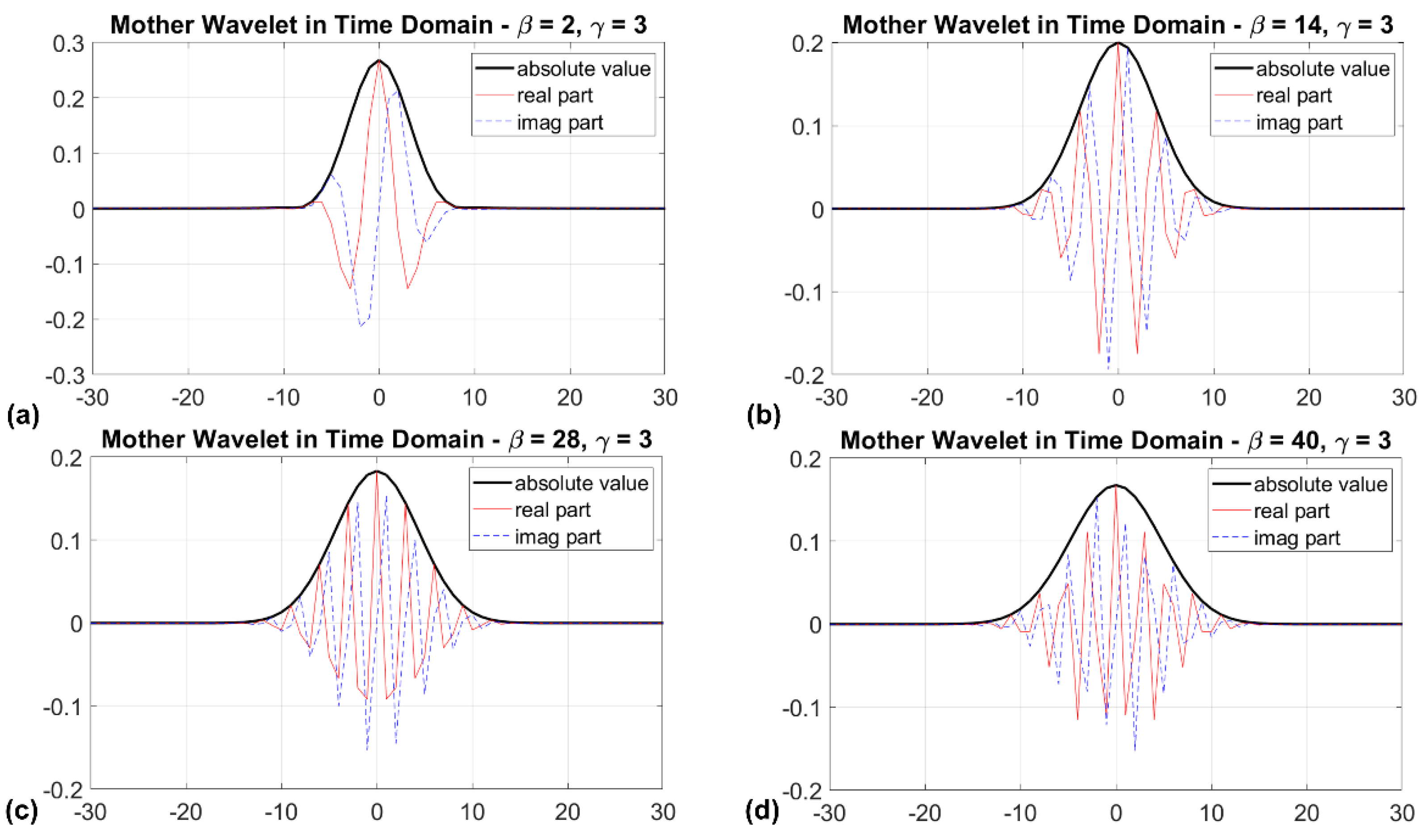
In detail, is directly proportional to the wavelet support along the time axis. Therefore, for constant , increasing implies a longer time–bandwidth. In turn, this increases the rate of the long-time decay and broadens the central portion of the resulting mother wavelet. For time–frequency analysis, a longer time duration, , implies more refined frequency resolution, , which is generally useful. This point will be better discussed in the Results (Section 5).
On the other hand, the gamma parameter controls the symmetry of the wavelet in time through the demodulate skewness [49]. Increasing for constant does not affect the time–bandwidth, but broadens the GWT envelope, making it more or less directional. For instance, if , the zeroth-order GWT corresponds to the Cauchy wavelet [51], which is strictly supported in a narrow convex cone in the time–frequency domain.
Different GWT shapes can better serve different purposes. These shapes can be grouped in a piecewise fashion as follows:
- 1.
- For constant (negative skewness), the time decay increases as the time–bandwidth (, thus ) increases.
- 2.
- For constant (positive skewness), the mother wavelet becomes more symmetric as increases.
Therefore, for , both the time decay and the wavelet symmetry increase with , and the resulting mother wavelet narrows in frequency and enlarges in time, with more oscillations under its envelope. This derives from the demodulate skewness of the GWT being null for gamma equal to 3; this results in a global maximum of the time/frequency concentration [46]—that is to say, it maximises the product of the time-domain and frequency-domain standard deviations, known as the Heisenberg’s area [40]. Again, all these aspects will be further investigated in a later Section.
4. The Experimental Case Study
The experimental recordings from a wind turbine have been used for the validation of the proposed entropy-based Condition Monitoring strategy. The dataset (described in detail in [52]) originates from an undisclosed onshore wind farm, located in Northern Sweden and consisting of 18 2.5 MW Nordex N100 wind turbines [53]. The continuous monitoring was performed over 46 consecutive months, acquiring 1.28 s-long time series (16,384 data points for a sampling frequency ) approximately every 12 h.
Specifically, Turbine #5 was considered here, as the only one (out of six installations included in the dataset) that suffered mechanical faults during the monitored timeframe.
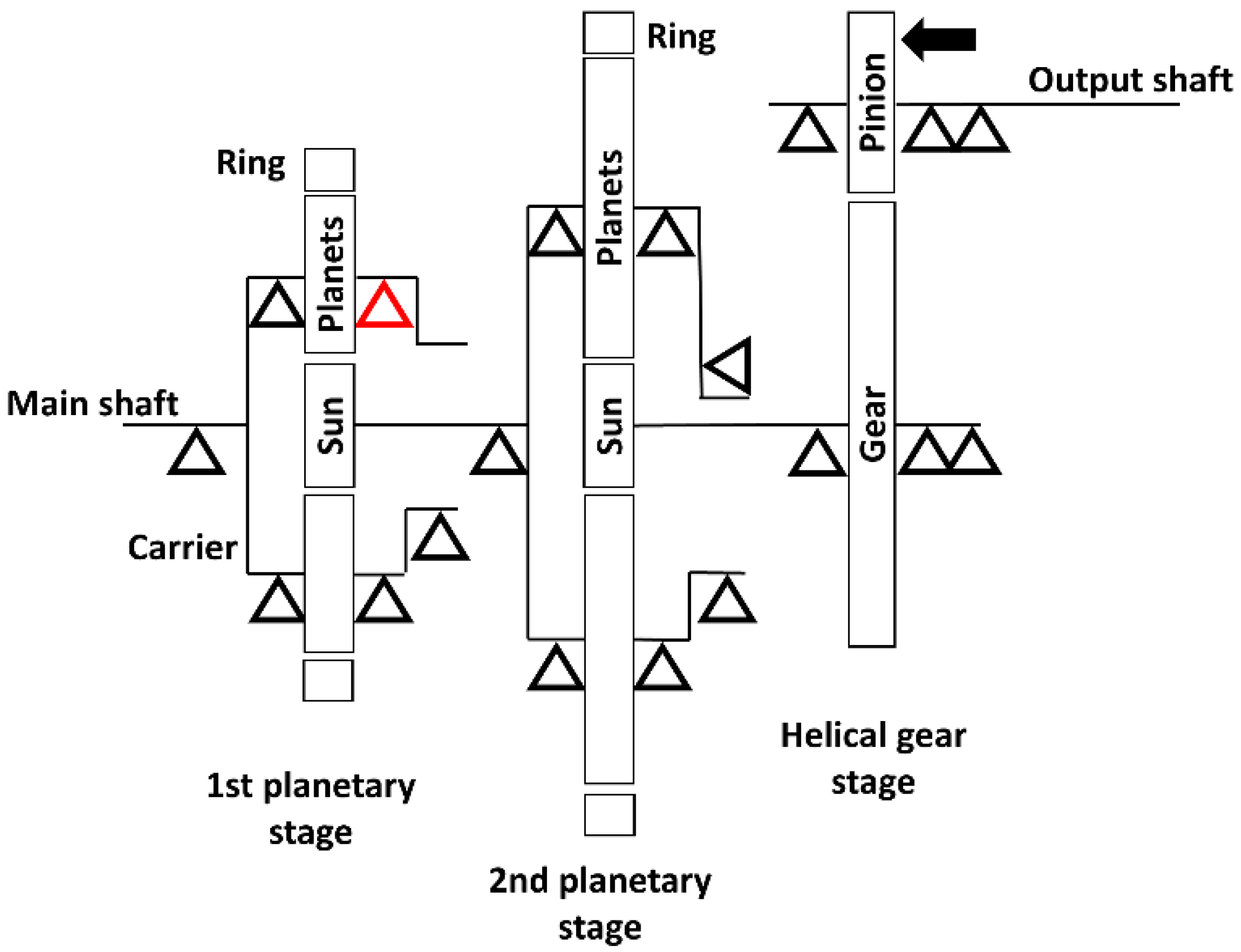
The vibration time series of interest were collected from an accelerometer, located and oriented as indicated by the black arrow in Figure 1 (which is based on the original schematics from [52]). This was mounted on the housing of the output shaft bearing of the turbine. The three-stage gearbox was made up of two sequential planetary gear stages, followed by a helical gear stage. The position of the bearing failure is highlighted in red in Figure 1. The damage consisted of an inner raceway failure on one of the four NSK RN2240 cylindrical roller bearings (CRBs) supporting one of the planets in the first planetary gear. From visual inspection after disassembly (refer to [52,53]), the most probable cause was identified as rolling fatigue-induced flaking (according to the NSK definition [54]), with a loss of material and the consequent rough and coarse texture extended over most of the contact surface. This caused the entire gearbox to be replaced after two years of operation.
Two signals of interest (portrayed in Figure 2) were defined by concatenating in chronological order some consecutive time histories (THs), recorded from Turbine #5 as described in Table 1 (the period column in Table 1 reports the time since the beginning of the continuous monitoring as year fractions). The concatenating procedure applied here reflects what was performed by Figueiredo et al. [55], to artificially generate a nonstationary experimental benchmark from stationary experimental recordings, emulating time-varying structural conditions with abrupt changes.
For signal #1, three segments were considered. These correspond to one recording (the first one) shortly before replacement and two acquisitions (the remaining two thirds) shortly after. These latter two were chosen since they are consecutive recordings with very similar rotational speeds (i.e., very similar external input; reported as cycles per minute).
Signal #1 was intended to study the effectiveness of the algorithm, presenting a discussion on parameter setting. For Machine Learning purposes, only the first tract was used as training data for the statistical modelling of the normal operating conditions (NOCs). The second and third parts of the signal provided the test points for the damage index.
For signal #2, a larger set of acquisitions were included. In this latter case, by considering only the optimised algorithm parameters, the intent was to address the full capabilities of the proposed approach when trained on more than one tract. Thus, signal #2 was evaluated on data with (almost) comparable rotational speeds before and after bearing damage. Specifically, the following segments were used:
- 1.
- seven consecutive tracts corresponding to 14 months before fault (the first five elements for training and the last two for validation),
- 2.
- the single tract already included in signal #1 plus five other nearby tracts immediately before fault (all included for further validation),
- 3.
- three recordings taken immediately after replacement, including the two already considered in signal #1 (all considered for testing),
- 4.
- other five segments acquired 7 months later (considered again for further testing).
The second part of Table 1 reports more details about these THs.
For both signal #1 and #2, the data, originally reported in terms of [], were standardised (subtracting the mean and dividing by the standard deviation, for each recording separately) to remove any potential issue related to the different amplitudes.
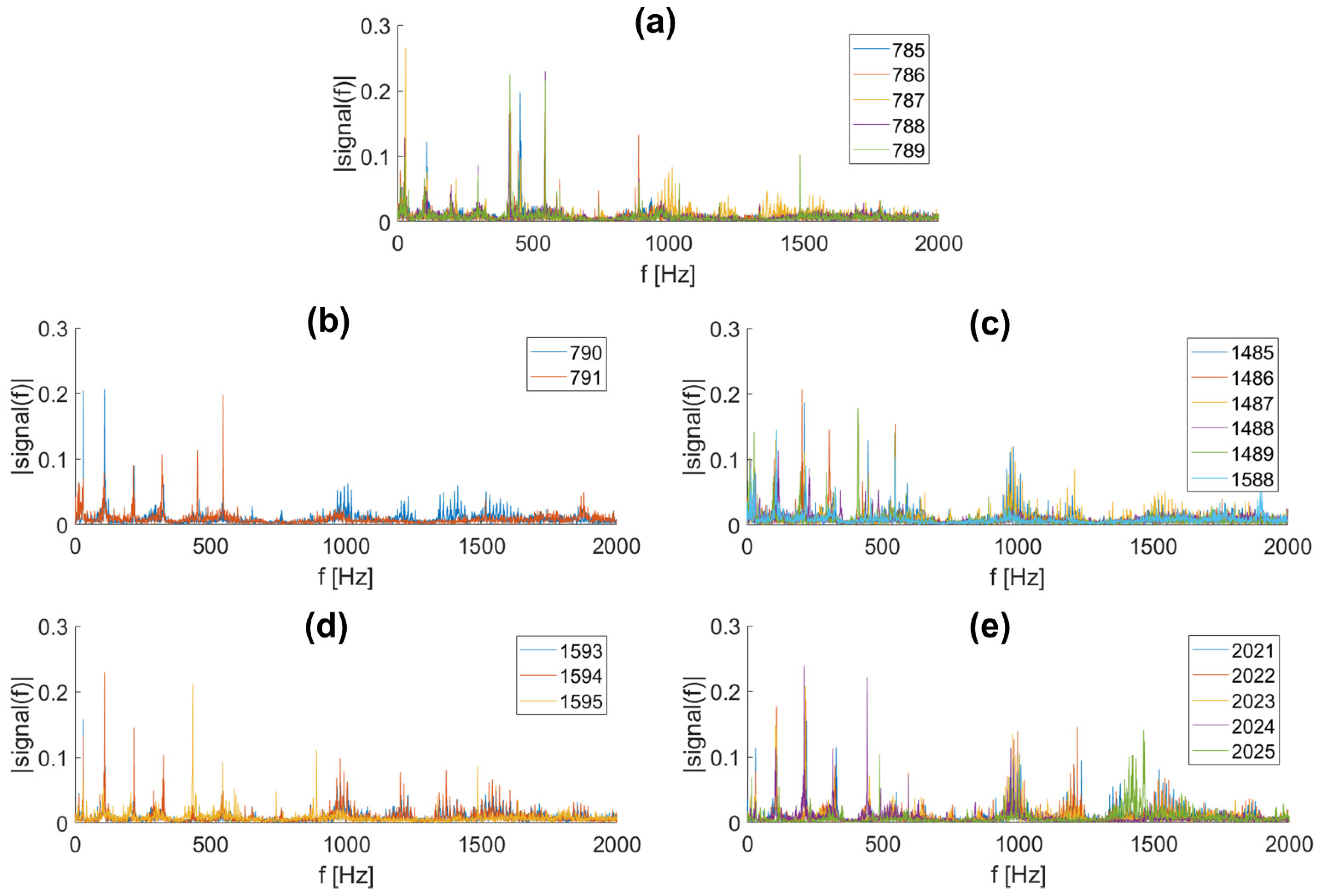
Figure 3 reports the Fast Fourier Transforms (FFT) of the five sets included in signal #2. One can notice that the multiple harmonic components of each acquisition do not allow for a simple comparison between the frequency content before and after the gearbox replacement. Thus, the common damage detection strategy based on the analysis of the frequency shift is hardly feasible in these circumstances. The same can be said for signal #1 as well since it comprises a subset of the segments of signal #2. Indeed, the limited reliability of FFT-based signal analysis for these typologies of bearing failure in wind turbine gearboxes was reported as well in [53].
5. Results
5.1. Signal #1
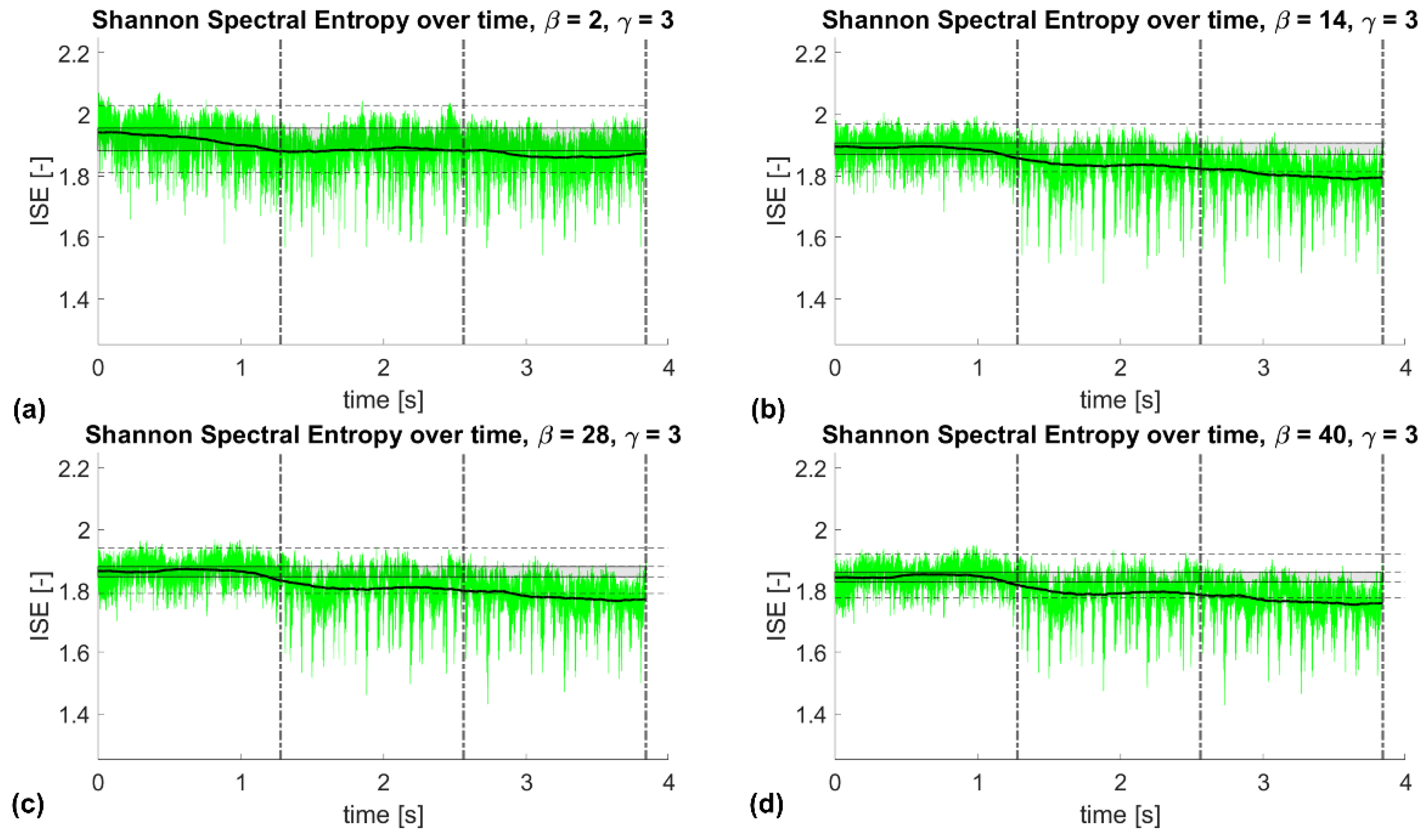
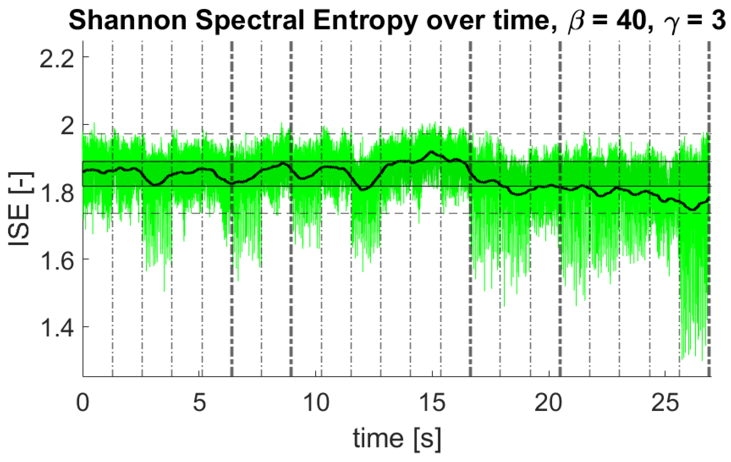
An example of results is reported in Figure 4. The green line corresponds to the Instantaneous Spectral Entropy, defined at any timestep. The two horizontal dashed lines correspond to the upper and lower bounds of the Gaussian distribution fitted over the ISE values of the training set, that is to say, and , where and correspond, in the same order, to the mean and standard deviation of the baseline tract, which is assumed to be almost stationary.
However, it was verified that these two thresholds were not optimal for anomaly detection. Indeed, as it can be seen, the value is quite unstable and subject to strong, rapid fluctuations. For this reason, a moving mean (calculated over a sliding window of 10,000 timesteps, i.e., 0.84 s) was preferred as a more stable indicator. This is indicated by the thick black line. The area shaded in grey corresponds to its expected values in ‘normal’ conditions, defined (similarly as before) as all points in between , i.e., with a 95.45% confidence of belonging to the same population as the training data points. One can see that, for the two test scenarios, the value of the moving average of generally deviated from the previously stationary conditions, trespassing the lower threshold. This can be used to perform automated and instantaneous fault detection.
The results portrayed in Figure 4 focus on a single value of symmetry () and varying . The effects of these two parameters have been thoroughly investigated. The findings will be discussed in the next subsection. However, the two points (1) and (2) highlighted above were encountered for any combination of and . This proves that the , especially when smoothed via a moving average with a properly sized window length, is, overall, effective and efficient as a time-dependent DSF, thus suitable for damage event detection.
5.1.1. Sensitivity Analysis for the GWT Parameters
Since the is a synthetic feature derived from the TF transform of the recorded signal, better time and frequency resolution will return more reliable results. Thus, it is essential to optimise the CWT settings. In the case investigated here, as mentioned in Section 3, the particular shape of the Generalised Morse (mother) Wavelet depends exclusively on the values considered for the doublet of parameters (). Therefore, to improve the capabilities of the proposed DSF, fine-tuning these two parameters becomes the most critical aspect of the whole procedure. For this reason, a dedicated sensitivity analysis has been performed.
The following cases were considered:
- 1.
- Symmetry equal to or .
- 2.
- varying from 2 to 40 in steps of 2.
Hence, a total of 140 combinations were analysed. The range of was defined to not exceed the suggested ratio [49]. Accordingly, (as the product of the lowest values of both and ) ranges from a minimum of 2 to a maximum of 160.
The aim of this optimisation is dual. For the training dataset, the data should behave as homogeneously as possible, to clearly define a NOCs model. This implies the signal stationarity (that is, constant mean and standard deviation ) and low variability (i.e., low sigma values).
For a constant gamma (in the previous example of Figure 4, ) increasing decreased the absolute value of both and . This latter point resulted in a narrower interval of confidence. In turn, this increased the sensitivity to damage as the threshold was lowered. The same trend was observed for all the other values of investigated here as well.
Regarding the testing part (second and third tracts of the concatenated signal), it is also noticeable how larger values increased the detectability of the fault condition, making a more marked transition from the “pre” to “post” damage insertion conditions. Again, this finding was verified for all values of
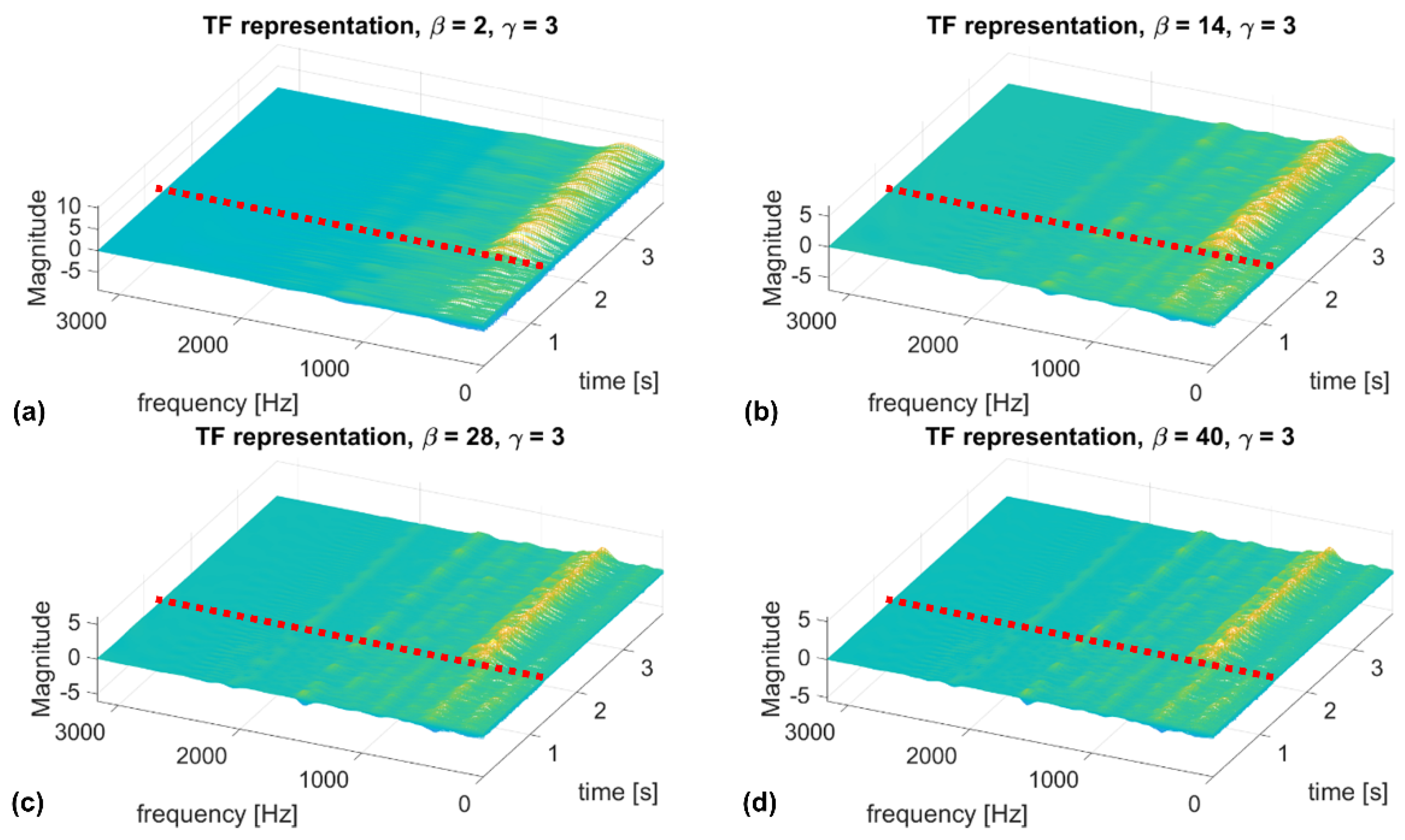
As anticipated, this derives from the detail of the TF representation. Figure 5 shows this point for the examples reported in Figure 4. Please note that to avoid any potential aliasing issue and considering the very high sampling frequency, the TF was truncated at (3200 Hz). The instant corresponding to the damage event is marked by the red dashed line.
One can see that the TF representation for and is clearly unreliable. The TF representations become more and more refined over the frequency axis as both (i) the length of the time support and (ii) the number of oscillations under the GWT envelope (and therefore the instantaneous frequency resolution) increase with (Figure 6). Since , this latter effect can be achieved by independently increasing or .
On the other hand, the effects of varying for constant can be summarised as follows.
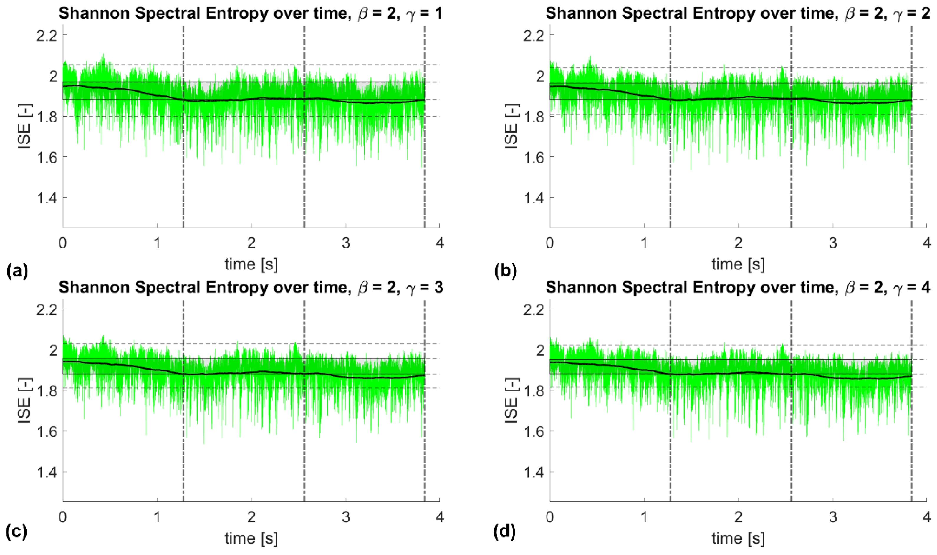
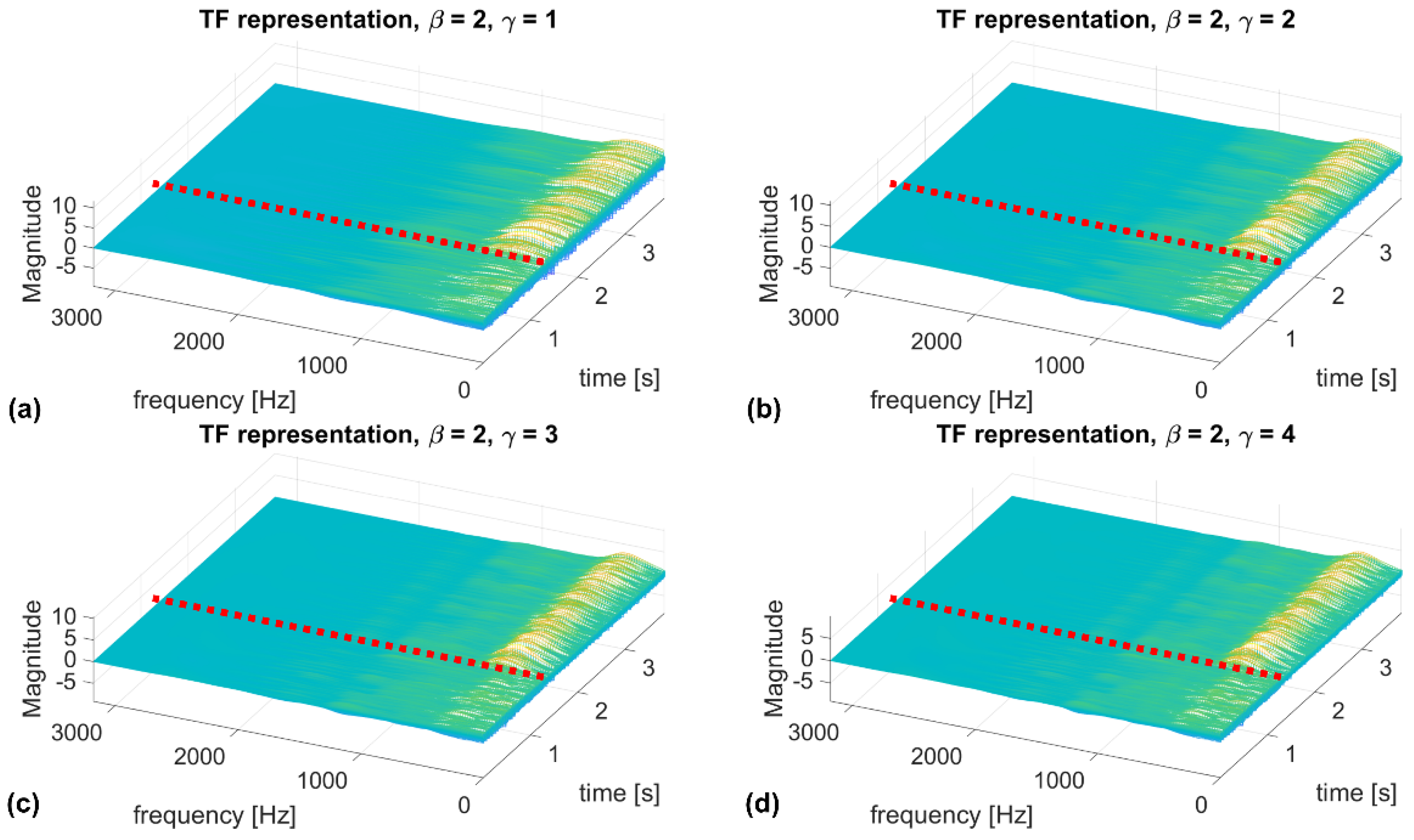
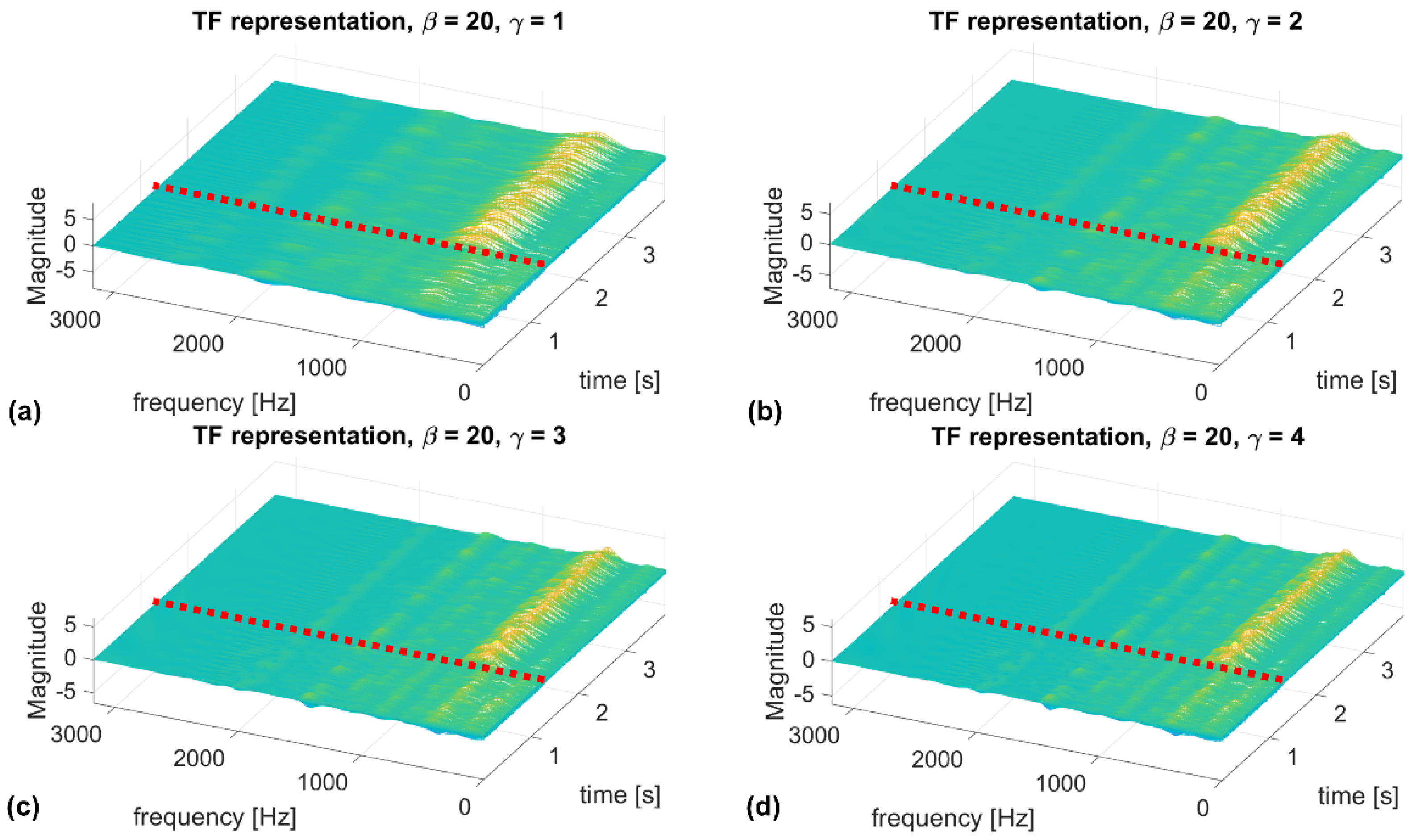
For any value of the symmetry value, lower values of ( in the example of Figure 7) have too coarse a frequency resolution and are thus almost unusable for the intended purposes, as it can be seen from the ISE values barely changing when moving from pre- to post-damage conditions. The corresponding TF representations are reported in Figure 8.
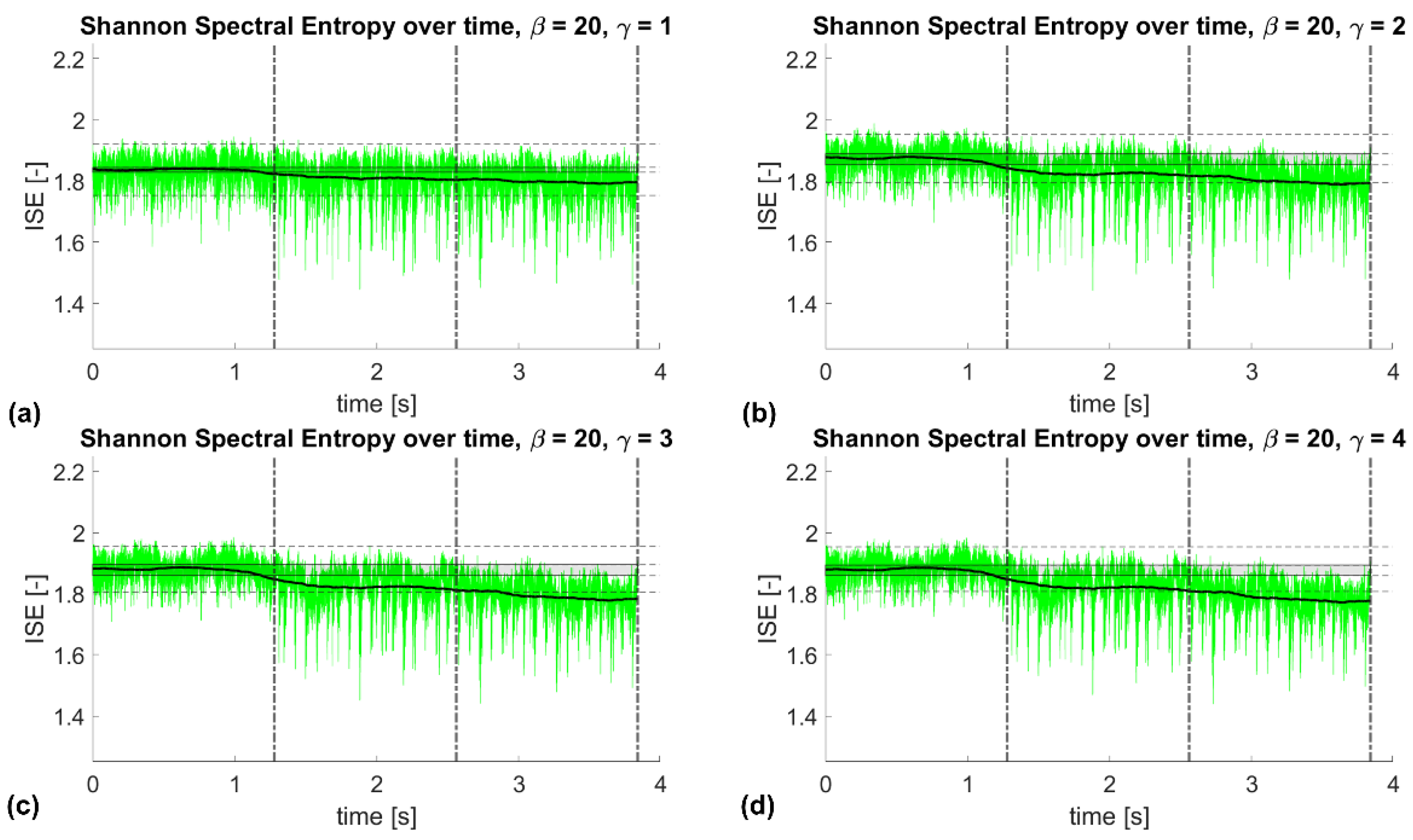
On the other hand, might return acceptable results, depending on the paired values. Generally speaking, returned distorted results, at least for the application investigated here. This is even more noticeable for , which were found to be unreliable for any value of . The results were instead less influenced by when the symmetry parameter was set as equal or larger than . By way of example, for , any gamma larger than 2 returned almost the same ISE(t) time history (see Figure 9; the corresponding TF transforms are reported in Figure 10).
In conclusion, the following points can be highlighted from this sensitivity analysis:
- 1.
- Values of are all deemed suitable. Increasing reduces the variability of the results, at least on the specific case study investigated here. Therefore, large values of are recommended, independently from the selected .
- 2.
- is suggested to avoid potential issues, even if were found to be suitable as well for the range of selected above, at least for this case study.
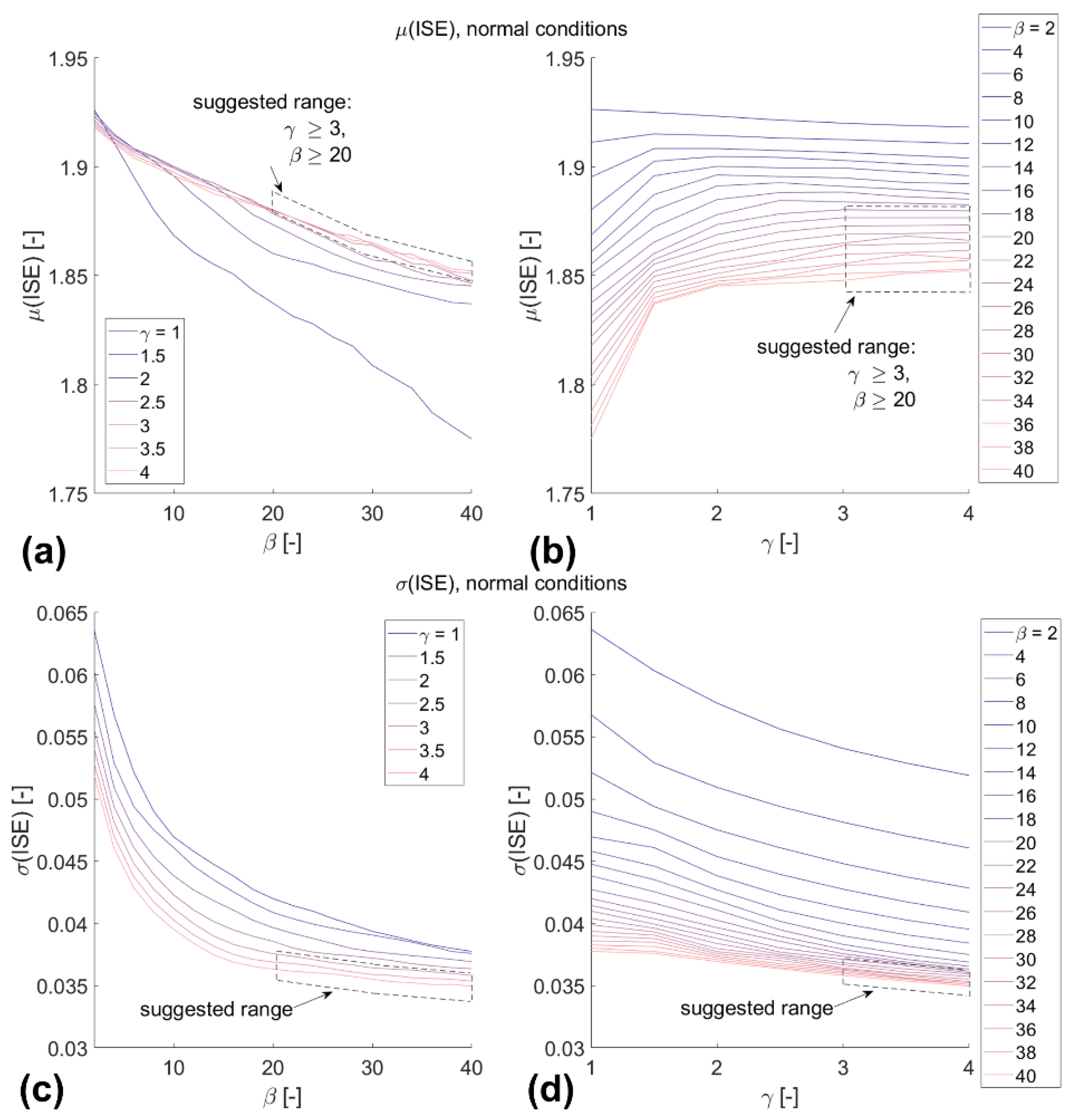
The suggested range is depicted in Figure 11, considering the mean and standard deviation of the ISE(t) computed over the NOCs. As mentioned previously, it is important to have stationary and low variance over the training dataset. This condition was confirmed for and . This selected area is also intended to avoid the undesired time-domain sidelobes and frequency-domain asymmetries that arise from very small time–bandwidth and large symmetry values.
5.1.2. Computational Efficiency
The computational effort required by the feature extraction procedure was further tested. This is essential for online SHM since the whole algorithm (feature extraction and threshold validation) should be performed in real-time, i.e., during the acquisition of an uninterrupted data stream. This is generally performed via a small moving window of recent history. Therefore, the computational time needed should be smaller than the considered time window.
Of the two main steps—TF transform and ISE() computation—the first one is the most demanding. Indeed, instantaneous SSE was performed (for the signal length considered here) in less than 0.6 s on average. This test, as well as the following ones, was performed on a laptop equipped with Windows 10 64-bit, Intel Core i7-7700HQ with CPU 2.80 GHz and 16.0 GB RAM, and MatLab R2020b.
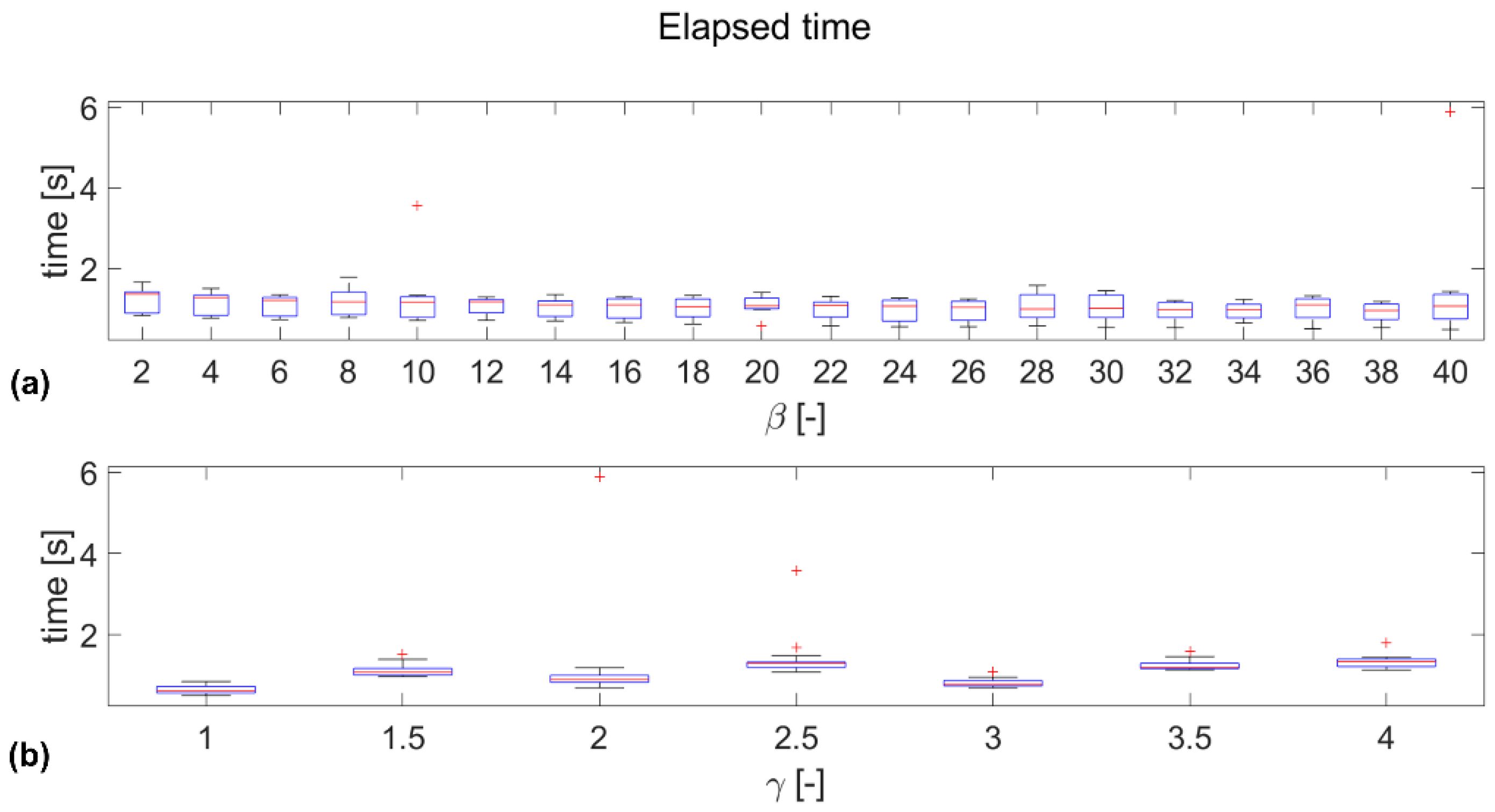
The CWT was found to be slightly longer to perform. As it can be seen from Figure 12, the elapsed time is mostly equal for any pair of values in the inspected ranges of the two GWT parameters. Except for (, ) and (, ), which lasted, respectively, for 5.8 s and 3.5 s, the CWT ran in less than 2.0 s everywhere else. Considering all cases, the overall mean elapsed time is about 1.08 s (1.02 s excluding the two outliers), with many combinations running in <1 s.
5.2. Signal #2
Figure 13 reports the results for the second, longer signal. and were set for this further study. One can notice that except for some tracts where the rotational speed was slightly higher than the average, the normality model—defined over five consecutive acquisitions—was validated almost everywhere on both the two validation sets (corresponding to, respectively, 14 months and immediately before the gearbox replacement). This indicates that the process has a certain level of robustness for relatively similar rotational speeds. Nevertheless, in some segments (more markedly in tract #1489, belonging to the second validation set, and to a lesser extent in #1487 and #1588, from the same set), three false positives were encountered. This can be explained since in binary classification, fine-tuning the classification algorithm parameters generally induces an increment in both the true positive and the false positive rates.
Immediately after the gearbox replacement, for a comparable wind speed, the ISE showed a noticeable decrease (as already described in the previous subsection). This behaviour was confirmed in the second test set, i.e., after more than seven months from the gearbox replacement. One can notice how some elements of the training and validation datasets have almost the same rotational speed but different ISE—e.g., tract #1588, the last one of the second validation set, and #2021, the first one of the second test set, correspond, respectively, to 785.45 and 786.29 cpm. This seems to indicate that the different output is not linked to any input variation but rather to structural changes.
6. Discussion
The experimental results show that the Instantaneous (Shannon) Spectral Entropy can be effectively used as a time-dependent damage index for Pattern Recognition-based SHM. However, one must use care in obtaining a time–frequency distribution which is as refined as possible, especially along the frequency axis. For this reason, a dedicated study was carried out.
High and values return the highest possible time duration and number of oscillations under the GWT envelope, which in turn grants the highest frequency resolution achievable at any instant. This greatly increases the damage detection capabilities of the proposed entropy-based approach. The performance reaches a plateau at a certain point, where the instantaneous power spectrum is refined enough, and further increasing does not significantly improve the final results. In this application, as mentioned previously, this was found at , , which therefore constitute the lower boundaries of the range of suggested settings. If one is interested in further improving the detectability of damage (by further shrinking the confidence interval around the normality model), according to these findings, increasing both and might be helpful. The optimal pair of (,) is, therefore, only limited by possible variations in the computational effort required. However, from the point of view of the computational effort, it was found that there is no relevant difference between different parameters.
However, due to the well-known optimal trade-off between time and frequency resolution (recalled in Section 3.2), it is strongly suggested to test as a first attempt, independently from the specific dataset, before increasing . Only if, after reaching , the resolution is still insufficient to obtain reliable estimates, the symmetry parameter should be further increased.
7. Conclusions
The Instantaneous Spectral Entropy (ISE) has been discussed as a potential time-dependent damage index. The Shannon Spectral Entropy (SSE) definition was used for this aim. The goal of this research was to perform damage event detection retrospectively on acquired vibration time histories, recorded from a wind turbine gearbox. The Continuous Wavelet Transform (CWT) was applied to define the time–frequency representation needed to extract the ISE. In this regard, a sensitivity analysis has been carried out on the parameters of the Generalised Morse Wavelet (GMW), to investigate their effects on the final results. Some suggestions were made based on the experimental data analysed here. However, further studies will be needed to assess these findings on different datasets, also considering different sampling frequencies and varying the duration of the recorded measurement time series.
The pure ISE was found to be significantly affected by spikes, i.e., very fast, short-termed transients of the instantaneous entropy. For this reason, its moving mean has been preferred as a more stable time-dependent index. The procedure successfully detected the occurrence of bearing faults on experimental data, recorded before and after a bearing failure and concatenated to emulate a time-varying structural condition. The moving mean of ISE returned some isolated false alarms as well; however, only an actual alteration of the machine condition caused a permanent deviation from the baseline.
As an entropy-based approach, the ISE is inherently limited by its dependence on the input force. That is to say, measurements corresponding to highly different wind speeds cannot be directly compared for anomaly detection. Future works will also include the automation of the selection procedure for acquisitions related to similar wind speeds.
Finally, the relatively low computational burden and rapid execution time suggest that the method can be further extended to real-time, online applications. This can be achieved using a small moving window of recent history over the data stream. These potential applications will be further investigated in future works as well.
Author Contributions
Conceptualization, M.C. and C.S.; methodology, M.C. and C.S.; software, M.C.; validation, M.C.; investigation, M.C.; resources, C.S.; data curation, M.C.; writing—original draft preparation, M.C.; writing—review and editing, C.S.; visualization, M.C.; supervision, C.S.; project administration, C.S. All authors have read and agreed to the published version of the manuscript.
Funding
This research received no external funding.
Institutional Review Board Statement
Not applicable.
Informed Consent Statement
Not applicable.
Data Availability Statement
The experimental data utilised for this research were retrieved from a public dataset, available at http://ltu.diva-portal.org/smash/record.jsf?pid=diva2%3A1244889&dswid=-2411 (accessed on 24 June 2021).
Acknowledgments
The Authors would like to thank S. Martin del Campo Barraza, F. Sandin, and D. Strömbergsson of the Luleå University of Technology for making their experimental data publicly available.
Conflicts of Interest
The authors declare no conflict of interest.
References
- New Energy Outlook 2020|BloombergNEF. Available online: https://about.bnef.com/new-energy-outlook/ (accessed on 23 June 2021).
- Olesen, G.B. Fast Transition to Renewable Energy with Local Integration of Large-Scale Windpower in Denmark; Publisher INFORSE: Aarhus, Denmark, 2014; Available online: https://inforse.org/europe/pdfs/Vision_DK_Fast_Transtions_RE_Denmark_article_EN_2014.pdf (accessed on 20 December 2021).
- Blaabjerg, F.; Ma, K. Future on power electronics for wind turbine systems. IEEE J. Emerg. Sel. Top. Power Electron. 2013, 1, 139–152. [Google Scholar] [CrossRef]
- Aloys, N.; Ariola, M. Wind in Power: 2016 European Statistics; WindEurope: Brussels, Belgium, 2017. [Google Scholar]
- International Renewable Energy Agency (IRENA). Renewable Energy Technologies: Cost Analysis Series; Volume 1: Power Sector, Issue 5/5; IRENA: Abu Dhabi, United Arab Emirates, 2012. [Google Scholar]
- European Wind Energy Association (EWEA). The Economics of Wind Energy; EWEA: Brussels, Belgium, 2009. [Google Scholar]
- Steffen, B.; Beuse, M.; Tautorat, P.; Schmidt, T.S. Experience Curves for Operations and Maintenance Costs of Renewable Energy Technologies. Joule 2020, 4, 359–375. [Google Scholar] [CrossRef]
- Myhr, A.; Bjerkseter, C.; Ågotnes, A.; Nygaard, T.A. Levelised cost of energy for offshore floating wind turbines in a lifecycle perspective. Renew. Energy 2014, 66, 714–728. [Google Scholar] [CrossRef] [Green Version]
- Shihavuddin, A.S.M.; Chen, X.; Fedorov, V.; Christensen, A.N.; Riis, N.A.B.; Branner, K.; Dahl, A.B.; Paulsen, R.R. Wind turbine surface damage detection by deep learning aided drone inspection analysis. Energies 2019, 12, 676. [Google Scholar] [CrossRef] [Green Version]
- Zhu, J.; Yoon, J.M.; He, D.; Bechhoefer, E. Online particle-contaminated lubrication oil condition monitoring and remaining useful life prediction for wind turbines. Wind Energy 2015, 18, 1131–1149. [Google Scholar] [CrossRef]
- Jasiüniené, E.; Raišutis, R.; Šliteris, R.; Voleišis, A.; Vladišauskas, A.; Mitchard, D.; Amos, M. NDT of wind turbine blades using adapted ultrasonic and radiographic techniques. Insight Non-Destr. Test. Cond. Monit. 2009, 51, 477–483. [Google Scholar] [CrossRef] [Green Version]
- Elforjani, M.; Mba, D. Condition monitoring of slow-speed shafts and bearings with Acoustic emission. Strain 2011, 47, 350–363. [Google Scholar] [CrossRef]
- Rumsey, M.A.; Musial, W. Application of Infrared Thermography Nondestructive Testing during Wind Turbine Blade Tests. J. Sol. Energy Eng. 2001, 123, 271. [Google Scholar] [CrossRef]
- Martin, R.W.; Sabato, A.; Schoenberg, A.; Giles, R.H.; Niezrecki, C. Comparison of nondestructive testing techniques for the inspection of wind turbine blades’ spar caps. Wind Energy 2018, 21, 980–996. [Google Scholar] [CrossRef]
- Rytter, A. Vibrational Based Inspection of Civil Engineering Structures. Ph.D. Dissertation, Aalborg Universitet, Aalborg, Denmark, 1993. [Google Scholar]
- Salameh, J.P.; Cauet, S.; Etien, E.; Sakout, A.; Rambault, L. Gearbox condition monitoring in wind turbines: A review. Mech. Syst. Signal Process. 2018, 111, 251–264. [Google Scholar] [CrossRef]
- Papatheou, E.; Dervilis, N.; Maguire, A.E.; Antoniadou, I.; Worden, K. A Performance Monitoring Approach for the Novel Lillgrund Offshore Wind Farm. IEEE Trans. Ind. Electron. 2015, 62, 6636–6644. [Google Scholar] [CrossRef] [Green Version]
- Papatheou, E.; Dervilis, N.; Maguire, A.E.; Campos, C.; Antoniadou, I.; Worden, K. Performance monitoring of a wind turbine using extreme function theory. Renew. Energy 2017, 113, 1490–1502. [Google Scholar] [CrossRef]
- Antoniadou, I.; Manson, G.; Dervilis, N.; Barszcz, T.; Staszewski, W.J.; Worden, K. Use of the Teager-Kaiser Energy Operator for Condition Monitoring of a Wind Turbine Gearbox. In Proceedings of the 25th International Conference on Noise and Vibration Engineering (ISMA), Leuven, Belgium, 17–19 September 2012. [Google Scholar]
- Ziaja, A.; Antoniadou, I.; Barszcz, T.; Staszewski, W.J.; Worden, K. Fault detection in rolling element bearings using wavelet-based variance analysis and novelty detection. J. Vib. Control 2016, 22, 396–411. [Google Scholar] [CrossRef]
- Powell, G.E.; Percival, I.C. A spectral entropy method for distinguishing regular and irregular motion of Hamiltonian systems. J. Phys. A Gen. Phys. 1979, 12, 2053–2071. [Google Scholar] [CrossRef]
- Pan, Y.N.; Chen, J.; Li, X.L. Spectral entropy: A complementary index for rolling element bearing performance degradation assessment. Proc. Inst. Mech. Eng. Part C J. Mech. Eng. Sci. 2009, 223, 1223–1231. [Google Scholar] [CrossRef]
- Ceravolo, R.; Lenticchia, E.; Miraglia, G. Use of Spectral Entropy for Damage Detection in Masonry Buildings in the Presence of Mild Seismicity. Proceedings 2018, 2, 432. [Google Scholar] [CrossRef] [Green Version]
- Ceravolo, R.; Lenticchia, E.; Miraglia, G. Spectral entropy of acceleration data for damage detection in masonry buildings affected by seismic sequences. Constr. Build. Mater. 2019, 210, 525–539. [Google Scholar] [CrossRef]
- Ceravolo, R.; Civera, M.; Lenticchia, E.; Miraglia, G.; Surace, C. Damage Detection and Localisation in Buried Pipelines using Entropy in Information Theory. In Proceedings of the 1st International Electronic Conference on Applied Sciences, Online, 10–30 November 2020; pp. 30–36. [Google Scholar]
- Ceravolo, R.; Civera, M.; Lenticchia, E.; Miraglia, G.; Surace, C. Detection and classification of multiple damages through entropy. Appl. Sci. 2021, 11, 5773. [Google Scholar] [CrossRef]
- Civera, M.; Surace, C. The Instantaneous Spectral Entropy for Real-time, Online Structural Health Monitoring. In Proceedings of the Damage Assessment of Structure (DAMAS), Shanghai, China, 29 October–1 November 2021. [Google Scholar]
- Worden, K.; Farrar, C.R.; Manson, G.; Park, G. The fundamental axioms of structural health monitoring. Proc. R. Soc. A Math. Phys. Eng. Sci. 2007, 463, 1639–1664. [Google Scholar] [CrossRef]
- Farrar, C.; Worden, K.; Park, G. Complexity: A New Axiom for Structural Health Monitoring? Los Alamos National Lab: Los Alamos, NM, USA, 2010. [Google Scholar]
- Pugno, N.; Surace, C.; Ruotolo, R. Evaluation of the Non-linear Dynamic Response to Harmonic Excitation of a Beam with Several Breathing Cracks. J. Sound Vib. 2000, 235, 749–762. [Google Scholar] [CrossRef] [Green Version]
- West, B.M.; Locke, W.R.; Andrews, T.C.; Scheinker, A.; Farrar, C.R. Applying concepts of complexity to structural health monitoring. In The Conference Proceedings of the Society for Experimental Mechanics Series; Springer: New York, NY, USA, 2019; Volume 6, pp. 205–215. [Google Scholar]
- Civera, M.; Boscato, G.; Zanotti Fragonara, L. Treed gaussian process for manufacturing imperfection identification of pultruded GFRP thin-walled profile. Compos. Struct. 2020, 254, 112882. [Google Scholar] [CrossRef]
- Farrar, C.R.; Worden, K. Structural Health Monitoring: A Machine Learning Perspective; John Wiley & Sons Ltd.: Chichester, UK, 2013. [Google Scholar]
- Civera, M.; Surace, C. A Comparative Analysis of Signal Decomposition Techniques for Structural Health Monitoring on an Experimental Benchmark. Sensors 2021, 21, 1825. [Google Scholar] [CrossRef]
- Fräser, K.F. An Overview of Health and Usage Monitoring Systems (HUMS) for Military Helicopters; Defence Science and Technology Organisation: Melbourne, Australia, 1994. [Google Scholar]
- Shannon, C.E. A Mathematical Theory of Communication. Bell Syst. Technol. J. 1948, 27, 379–423. [Google Scholar] [CrossRef] [Green Version]
- Bromiley, P.A.; Thacker, N.A.; Bouhova-Thacker, E. Shannon Entropy, Renyi Entropy, and Information; The University of Manchester: Manchester, UK, 2010. [Google Scholar]
- Rioul, O.; Vetterli, M. Wavelets and signal processing. IEEE Signal Process. Mag. 1991, 8, 14–38. [Google Scholar] [CrossRef] [Green Version]
- Daubechies, I.; Bates, B.J. Ten Lectures on Wavelets; Society for Industrial and Applied Mathematics: Philadelphi, PA, USA, 1992; ISBN 0898712742. [Google Scholar]
- Mallat, S. A Wavelet Tour of Signal Processing; Elsevier Inc.: San Diego, CA, USA, 2009; ISBN 9780123743701. [Google Scholar]
- Sifuzzaman, M.; Islam, M.R.; Ali, M.Z. Application of Wavelet Transform and its Advantages Compared to Fourier Transform. J. Phys. Sci. 2009, 13, 121–134. [Google Scholar]
- Surace, C.; Di Torino, P.; Ruotolo, R. Crack Detection of a Beam Using the Wavelet Transform. In Proceedings of the The International Society For Optical Engineering, Turin, Italy, 10 January 1994. [Google Scholar]
- Taha, M.M.R.; Noureldin, A.; Lucero, J.L.; Baca, T.J. Wavelet Transform for Structural Health Monitoring: A Compendium of Uses and Features. Struct. Health Monit. Int. J. 2006, 5, 267–295. [Google Scholar] [CrossRef]
- Poularikas, A.D. Transforms and Applications Handbook; CRC Press: Boca Raton, FL, USA, 1996. [Google Scholar]
- Silik, A.; Noori, M.; Altabey, W.A.; Ghiasi, R.; Wu, Z. Comparative Analysis of Wavelet Transform for Time-Frequency Analysis and Transient Localization in Structural Health Monitoring. Struct. Durab. Health Monit. 2021, 15, 1–22. [Google Scholar] [CrossRef]
- Lilly, J.M.; Olhede, S.C. Generalized morse wavelets as a superfamily of analytic wavelets. IEEE Trans. Signal Process. 2012, 60, 6036–6041. [Google Scholar] [CrossRef] [Green Version]
- Wang, P.; Gao, J. Extraction of instantaneous frequency from seismic data via the generalized Morse wavelets. J. Appl. Geophys. 2013, 93, 83–92. [Google Scholar] [CrossRef]
- Huang, F.; Chen, D.; Zhou, L. Rotating machine fault diagnosis based on correlation filtering and reconstructed Morlet wavelet power spectral entropy. In Proceedings of the 2020 6th International Conference on Mechanical Engineering and Automation Science, ICMEAS 2020, Moscow, Russia, 29–31 October 2020; pp. 61–65. [Google Scholar]
- Lilly, J.M.; Olhede, S.C. Higher-Order Properties of Analytic Wavelets. IEEE Trans. Signal Process. 2008, 57, 146–160. [Google Scholar] [CrossRef] [Green Version]
- Daubechies, I.; Paul, T. Time-frequency localisation operators-a geometric phase space approach: II. The use of dilations. Inverse Probl. 1988, 4, 661–680. [Google Scholar] [CrossRef] [Green Version]
- Olhede, S.C.; Walden, A.T. Generalized Morse Wavelets. IEEE Trans. Signal Process. 2002, 50, 2661–2670. [Google Scholar] [CrossRef] [Green Version]
- Martin-Del-campo, S.; Sandin, F.; Strömbergsson, D. Dictionary learning approach to monitoring of wind turbine drivetrain bearings. Int. J. Comput. Intell. Syst. 2021, 14, 106–121. [Google Scholar] [CrossRef]
- Strömbergsson, D.; Marklund, P.; Berglund, K.; Larsson, P.E. Bearing monitoring in the wind turbine drivetrain: A comparative study of the FFT and wavelet transforms. Wind Energy 2020, 23, 1381–1393. [Google Scholar] [CrossRef] [Green Version]
- NSK Company. New Bearing Doctor—Maintenance of Bearings; Publisher NSK Company: Maidenhead, UK, 2009; Available online: https://www.nsk-literature.com/en/new-bearing-doctor-maintenance/offline/download.pdf (accessed on 20 December 2021).
- Figueiredo, E.; Park, G.; Figueiras, J. Structural Health Monitoring Algorithm Comparisons Using Standard Data Sets; Los Alamos National Lab. (LANL): Los Alamos, NM, USA, 2009. [Google Scholar]
Figure 1.
Schematics of the three-stage gearbox, with the damaged bearing highlighted in red and the position and direction of the output channels indicated by the black arrow.
Figure 1.
Schematics of the three-stage gearbox, with the damaged bearing highlighted in red and the position and direction of the output channels indicated by the black arrow.

Figure 2.
The investigated signals: (a) #1, (b) #2. Data standardised as . In (a), the dot-dashed vertical lines represent the three concatenated segments. In (b), the thick dot-dashed vertical lines enclose the segments considered for the training set, the two validation sets, and the two test sets, in this order (see Table 1). The single segments are separated by thin vertical lines.

Figure 3.
Fast Fourier Transforms (FFTs) of the segments of each set included in signal #2. (a): training set; (b): validation set #1; (c): validation set #2; (d): test set #1; (e): test set #2.
Figure 3.
Fast Fourier Transforms (FFTs) of the segments of each set included in signal #2. (a): training set; (b): validation set #1; (c): validation set #2; (d): test set #1; (e): test set #2.

Figure 4.
Resulting ISE (signal #1). Values for and equal to (a) (b) , (c) , and (d) 40.

Figure 5.
Time–frequency distributions corresponding to the results shown in Figure 4 ( and equal to (a) (b) , (c) , and (d) 40).
Figure 5.
Time–frequency distributions corresponding to the results shown in Figure 4 ( and equal to (a) (b) , (c) , and (d) 40).

Figure 6.
Mother wavelets (in the time domain) corresponding to the results shown in Figure 4 ( and equal to (a) (b) , (c) , and (d) 40).
Figure 6.
Mother wavelets (in the time domain) corresponding to the results shown in Figure 4 ( and equal to (a) (b) , (c) , and (d) 40).

Figure 7.
Resulting ISE (signal #1). Values for and equal to (a) (b) , (c) , and (d) 4.

Figure 8.
Time–frequency distributions corresponding to the results shown in Figure 7 ( and equal to (a) (b) , (c) , and (d) 4).
Figure 8.
Time–frequency distributions corresponding to the results shown in Figure 7 ( and equal to (a) (b) , (c) , and (d) 4).

Figure 9.
Resulting ISE (signal #1). Values for. and equal to (a) (b) , (c) , and (d) 4.

Figure 10.
Time–frequency distributions corresponding to the results shown in Figure 9 ( and equal to (a) (b) , (c) , and (d) 4).
Figure 10.
Time–frequency distributions corresponding to the results shown in Figure 9 ( and equal to (a) (b) , (c) , and (d) 4).

Figure 11.
Trends of ISE values for the normal conditions. (a): for varying ; (b): for varying ; (c): for varying ; (d): for varying .
Figure 11.
Trends of ISE values for the normal conditions. (a): for varying ; (b): for varying ; (c): for varying ; (d): for varying .

Figure 12.
Boxplot of the CWT execution time. (a): as a function of . (b): as a function of .

Figure 13.
Resulting ISE (signal #2). Values for. and .


Table 1.
The concatenated recordings, as reported in the experimental database 1.
| Signal #1 | ||||
|---|---|---|---|---|
| ID number | Period of recording [years] | Rotational speed [cpm] | Structural conditions | Set |
| 1588 | 1.9972 | 785.45 | Immediately pre-replacement | Training |
| 1593 | 2.0040 | 783.61 | Immediately post-replacement | Test |
| 1594 | 2.0054 | 783.18 | Immediately post-replacement | Test |
| Signal #2 | ||||
| ID number | Period of recording [years] | Rotational speed [cpm] | Structural conditions | Set |
| 785 | 0.7936 | 777.79 | More than one year pre-replacement | Training |
| 786 | 0.7988 | 714.90 | >1 year pre-replacement | Training |
| 787 | 0.7989 | 779.824 | >1 year pre-replacement | Training |
| 788 | 0.8080 | 708.74 | >1 year pre-replacement | Training |
| 789 | 0.8205 | 711.63 | >1 year pre-replacement | Training |
| 790 | 0.8208 | 785.33 | >1 year pre-replacement | Validation #1 |
| 791 | 0.8217 | 774.61 | >1 year pre-replacement | Validation #1 |
| 1485 | 1.8480 | 768.34 | Immediately pre-replacement | Validation #2 |
| 1486 | 1.8493 | 733.26 | Immediately pre-replacement | Validation #2 |
| 1487 | 1.8507 | 772.99 | Immediately pre-replacement | Validation #2 |
| 1488 | 1.8521 | 832.43 | Immediately pre-replacement | Validation #2 |
| 1489 | 1.8537 | 706.29 | Immediately pre-replacement | Validation #2 |
| 1588 2 | 1.9972 | 785.45 | Immediately pre-replacement | Validation #2 |
| 1593 3 | 2.0040 | 783.61 | Immediately post-replacement | Test #1 |
| 1594 3 | 2.0054 | 783.18 | Immediately post-replacement | Test #1 |
| 1595 | 2.0076 | 744.07 | Immediately post-replacement | Test #1 |
| 2021 | 2.5995 | 786.29 | More than half a year post-replacement | Test #2 |
| 2022 | 2.6009 | 777.30 | >1/2 year post-replacement | Test #2 |
| 2023 | 2.6023 | 772.13 | >1/2 year post-replacement | Test #2 |
| 2024 | 2.6036 | 757.19 | >1/2 year post-replacement | Test #2 |
| 2025 | 2.6050 | 836.38 | >1/2 year post-replacement | Test #2 |
1 http://ltu.diva-portal.org/smash/record.jsf?pid=diva2%3A1244889&dswid=-2411 (accessed on 24 June 2021). 2 Already included in signal #1 for training. 3 Already included in signal #1 for testing.
Publisher’s Note: MDPI stays neutral with regard to jurisdictional claims in published maps and institutional affiliations. |
© 2022 by the authors. Licensee MDPI, Basel, Switzerland. This article is an open access article distributed under the terms and conditions of the Creative Commons Attribution (CC BY) license (https://creativecommons.org/licenses/by/4.0/).
Share and Cite
MDPI and ACS Style
Civera, M.; Surace, C. An Application of Instantaneous Spectral Entropy for the Condition Monitoring of Wind Turbines. Appl. Sci. 2022, 12, 1059. https://0-doi-org.brum.beds.ac.uk/10.3390/app12031059
AMA Style
Civera M, Surace C. An Application of Instantaneous Spectral Entropy for the Condition Monitoring of Wind Turbines. Applied Sciences. 2022; 12(3):1059. https://0-doi-org.brum.beds.ac.uk/10.3390/app12031059
Chicago/Turabian StyleCivera, Marco, and Cecilia Surace. 2022. "An Application of Instantaneous Spectral Entropy for the Condition Monitoring of Wind Turbines" Applied Sciences 12, no. 3: 1059. https://0-doi-org.brum.beds.ac.uk/10.3390/app12031059
Note that from the first issue of 2016, this journal uses article numbers instead of page numbers. See further details here.