Causally Remove Negative Confound Effects of Size Metric for Software Defect Prediction

Abstract

Software defect prediction technology can effectively detect potential defects in the software system. The most common method is to establish machine learning models based on software metrics for prediction. However, most of the prediction models are proposed without considering the confounding effects of size metric. The size metric has unexpected correlations with other software metrics and introduces biases into prediction results. Suitably removing these confounding effects to improve the prediction model’s performance is an issue that is still largely unexplored. This paper proposes a method that can causally remove the negative confounding effects of size metric. First, we quantify the confounding effects based on a causal graph. Then, we analyze each confounding effect to determine whether they are positive or negative, and only the negative confounding effects are removed. Extensive experimental results on eight data sets demonstrate the effectiveness of our proposed method. The prediction model’s performance can, in general, be improved after removing the negative confounding effects of size metric.

1. Introduction

With the development of information technology, various software systems make people’s daily lives highly informative. These software systems were closely related to the country’s economic revitalization and social development, and therefore ensuring the quality of the software system is crucial. Software defects are an essential factor that affects software system quality [1,2], and software developers should search for software defects to improve the software system quality [3]. In particular, the current software development process is often agile. Software practitioners must often launch software products within a limited time, making it impossible to set aside enough time for software testing; therefore, it is a luxury for software products to be thoroughly tested. Software defect prediction can effectively predict potential software defects, allowing testers to devote more resources to software modules that are more likely to have defects.

Software defect prediction is an effective means to discover potential software defects. The most commonly used method of software defect prediction is to use software metrics to establish the predictive model based on machine learning technology [4,5,6,7,8]. Many classic machine learning models achieved excellent results in software defect prediction, such as Logistic Regression (LR) [9], Support Vector Machine (SVM) [10], Neural Network (NN) [11], Naive Bayes (NB) [12].

However, in traditional machine learning, there is an assumption that there are weak correlations between variables, and these correlations cause confounding and bring biases into the prediction results [13,14]. Due to the inherent characteristics of software metrics, the size metric has undesirable correlations with other metrics. These undesirable correlations bring redundancy and make the size metric a powerful confounder [15]. The confounder size metric could conceal the actual predictive ability of the metrics, making the prediction result unsatisfactory. Emma et al. [15] first examined the confounding effects of size metric and strongly recommended that the confounding effects of size metric should be removed before building the predictive model. Later, other researchers [16,17] also paid attention to this issue. However, they focused more on verifying the existence of the confounding effects rather than proposing a method to remove them.

The Linear Confounding Effect Removal Method (LCERM) [17] was generally applied in the medical field. This method represents the confounding effects of the linear regression model and removes the confounding effects directly from the original data. However, it is not suitable for the field of software defect prediction for two reasons: one is that linear-based methods cannot express well the relationship between software metrics; there exist nonlinear correlations between the determined software metrics, so the linear method’s applicability is poor. The second is that removing confounding effects is not certainly conducive to software defect prediction. The bias caused by confounding could be a positive or negative bias. Positive bias is beneficial for prediction; negative bias is the opposite. Our ultimate goal is to improve the prediction model’s performance, and therefore we should retain the positive biases and remove the negative biases.

This paper proposes a Causally Removing Negative Confound Effects Method (CRNCEM). Under the causal graph [18] framework, the proposed removal method meets theoretical interpretability and empirical effectiveness. Concretely, first, we appropriately quantify the confounding effects according to the structure of the causal graph. The quantification process applies a Generalized Additive Model (GAM) [19], which can analyze the complex nonlinear relationship between metrics. Second, we selectively remove negative confounding effects. We use correlation analysis to determine whether each confounding has a negative or positive effect. The negative confounding effects are subtracted from the original data to get nonconfounding data. The revised data could be used to establish the defect prediction model. On eight datasets, we verified the effectiveness of the CRNCEM. In the experiments, LR was applied as the basic classify. Compared with that of LR and LCERM + LR, the CRNCEM + LR has an improvement of 1.3–5.2% under the F1 score (F1) indicator, and the CRNCEM + LR performs better than NN predictive model. The experimental results show that our method effectively improves the performance of the prediction model.

Our main contributions include the following aspects:

• We focused on a seldom studied issue: removing the confounding effects of size metric for software defect prediction. These confounding effects are objective and bring biases in the prediction results.
• We are the first to consider selectively removing confounding effects. We proposed the CRNCEM, which causally quantifies the confounding effect, and then determines and removes the negative effect that is not conducive to defect prediction.
• We conduct comprehensive experiments, and the results demonstrate the superiority of CRNCEM for software defect prediction.

The rest of the paper is organized as follows: Section 2 reviews related works; Section 3 interprets the proposed CRNCEM; Section 4 introduces experiments and the analysis of the results; and Section 5 is the conclusion.

2. Related Works

The software engineering research community is very interested in software defect prediction and made many efforts to use software metrics to predict software defects [4,5,6,7,8]. Software defect prediction is a two-category task: software modules that contain potential defects must be distinguished from the remainder. Researchers generally used machine learning techniques to establish prediction models. Many classic machine learning methods are excellent in software defect prediction content, such as LR [9,20,21,22], NN [11], SVM [10], and NB [12]. The LR is the most commonly used classification method, and it also achieved the best predictive performance [23,24,25]. The most well-known and commonly used LR for software defect prediction is a two-step LR model [26,27,28]. The first step is to select metrics that are suitable indicators for defect prediction. More suitable indicators have better defect prediction performance, since not all software metrics have useful predictability. The second step involves using the metrics selected in the previous step to establish a multivariate LR model for prediction.

However, these studies did not consider the confounding effects of size metric. To the best of our knowledge, Emma et al. [15] were the first to paid attention to the confounding effects of size metric. They questioned the traditional modeling methods, and they also believed that the size metric would obscure the predictive ability of software metrics and bring biases into the prediction results. Based on a C++-based telecommunications software, they empirically verified their hypothesis. The results showed that size metric has confounding effects on most software metrics. Moreover, they concluded that the size metric is a powerful confounder, and they strongly suggested that size metric must be controlled before establishing a defect prediction model. However, due to the use of threshold-based experimental methods, the selected threshold affects the experimental results. Later, Zhou et al. [16] proposed a method to test the confounding effect based on linear regression. They conducted experiments on a general data set containing 55 software metrics and came to the same conclusion as Emma et al. Still, the normality assumptions are rarely specious when modeling software defects with linear regression [29]. After that, a method based on logistic regression was proposed [29]. In this method, a bivariate logistic regression was used to evaluate the relationship between a single software metric and defect-proneness with and without the size metric. Zhou et al. [17] introduced a mathematical model based on logistic regression to detect whether and how confounding affects the prediction results. They also applied a linear regression-based confounding removal method for software defect prediction. After removing the confounding effects of size metric, the LR-based prediction model performed well under the effort-aware indicators. However, their model did not have universal applicability under commonly used indicators for machine learning models such as F1. We followed their idea about how to remove the confounding effects from metrics. Unlike the linear-based method they used, we applied the nonlinear method to quantify and remove only the negative confounding effects.

3. Method

3.1. Confounding Effects of Size Metric

The concept of confounding is popular in the field of health sciences [30]. It refers to the situation where the relationship between variables is erroneously obscured or emphasized by a third variable [31]. The third variable is usually called a confounder.

In the field of software defect prediction, size metric is a significant confounder. Size metric may lead to overestimating or underestimating the predictive ability of software metrics to defect-proneness, depending on the direction and magnitude of its confounding effects [32].

We use a causal graph to illustrate a confounding effect of size metric, as shown in Figure 1. To simplify the description, we use variable Z to represent the size metric, X to represent one other software metric, and Y to represent defect-proneness. Software metrics and defect-proneness are related, and software metrics are used to predict defect-proneness; therefore, there are unidirectional edges XY and ZY. The unidirectional edge represents the causal belief that means that X and Z are the antecedents to Y. The size metric and the software metric have a not weak correlation, so there is bidirectional edge ZX. The bidirectional edge represents a general association. Therefore, there are two paths connecting X and Y, which are XY and XZY. The direct path XY represents the true relationship between X and Y. The indirect path XZY contains the confounding effect of Z. When exploring the relationship between X and Y, both paths are considered. As such, the obtained conclusion includes the confounding effect. To explore the true relationship between X and Y, we must control Z to block path XZY. After that, only path XY is connected. Then, the relationship between X and Y will not be affected by Z.

3.2. Method of Causally Removing Negative Confounding Effect

The prerequisite for the confounding effects of the size metric is that it is related to other software metrics. In Figure 1, Z can explain part of X. If there is no this related part, then there will be no edge between X and Z, so Z will not confound the correlation between X and Y. We denote the unrelated part in X as X${}^{\prime }$. Hence, X${}^{\prime }$ is the part of X that has nothing to do with Z, and the correlation between X${}^{\prime }$ and Y is not affected by the confounder Z. Based on the above analysis, we quantify the confounding effects of size metric. Then, we use the correlation-based method to analyze the direction of the confounding effects. We know that high correlation usually means the great predictive ability of one software metric for the software defect. We compare CorXY (the correlation between X and Y) with CorX${}^{\prime }$Y (the correlation between X${}^{\prime }$ and Y). If CorXY is the larger one, it means that Z hurts the predictive ability of X; in other words, confounding has a negative effect. This confounding effect should be removed. On the contrary, if CorX${}^{\prime }$Y is the larger one, it means that Z enhances the predictive ability of X, and the confounding has a positive effect. This confounding effect should be retained.

Based on the above, we propose the CRNCEM, and Algorithm 1 presents the pseudocode. The CRNCEM is generally divided into two steps. The first step is to quantify the value of the confounding effect; the second step is to analyze the confounding effect, and then remove the negative confounding effect, which is not conducive to defect prediction. For each metric except the size metric:

Step 1:

Quantify the confounding effect

Since there are complex nonlinear relationships between the size metric and other metrics, we choose a generalized additive model (GAM) to quantify the confounding effects. GAM is a data-driven model with a strong ability to analyze the nonlinear relationship and does not require any assumptions between variables. The mathematical expression of GAM is as shown:

$$B={\beta }_0+\sum _{i=1}^k{f}_i\left(A_i\right)$$

(1)

in which coefficients ${\beta }_0$ is a constant, function $f_i\left(A_i\right)$ is a smoothing function determined by the explained variables themselves [19], and K is the number of independent variables.

First, we use the GAM to fit a metric by size metric, as shown in formula (2).

$$X={\beta }_0+f_i\left(Z\right)$$

(2)

Then, we use the size metric to predict that metric. As shown in formula (3), $\widehat{X}$ means the prediction value. Let$\widehat{{\beta }_0}$ and $\widehat{f}$ be the sample estimates for ${\beta }_0$ and f, respectively. $\widehat{X}$ is the explained part of X.

$$\widehat{X}=\widehat{{\beta }_0}+\widehat{f_i}\left(Z\right)$$

(3)

Therefore, X${}^{\prime }$ can be expressed as X minus the explained part of X, as shown in formula (4). Indeed, X${}^{\prime }$ is equal to the prediction error [33].

$$X^{\prime }=X-\widehat{X}$$

(4)

Step 2:

Remove the negative confounding effect

Pearson coefficient is used to analyze the confounding effect. Pearson coefficient is the most commonly used statistics indicator for the correlation between variables. The formula is as follows:

$$p(X,Y)=\frac{Cov(X,Y)}{\sqrt{Var\left[X\right]Var\left[Y\right]}}$$

(5)

in which Cov[] represents covariance, Var[] representative variance.

We use formula (5) to calculate the Pearson coefficients between the original metric X and defect-proneness Y, signed as $p_{xy}$; Pearson coefficients between the nonconfounding metric X${}^{\prime }$ and defect-proneness Y, signed as $p_{x^{\prime }y}$. Compare $p_{xy}$ and $p_{x^{\prime }y}$, and if $p_{xy}$ is larger, we keep the original X; otherwise, replace X with X${}^{\prime }$.

Algorithm 1 CRNCEM.

Input: Original data (X presents a software metric; Z presents size metric; Y presents defect-proneness) Output: Revised data 1: for Each metric do 2:    Using GAM to fit X by Z, obtain $X:=\widehat{{\beta }_0}+\widehat{f_i}\left(Z\right)$ 3:    Predict X by Z, obtain $\widehat{X}=\widehat{{\beta }_0}+\widehat{f_i}\left(Z\right)$ 4:    Calculate X’$=X-\widehat{X}$ 5:    Calculate Pearson coefficient $p_{xy}$ and $p_{x^{\prime }y}$ 6:    if $p_{xy}$ < $p_{x^{\prime }y}$ then 7:      replace X with X${}^{\prime }$ 8:    end if 9: end for

4. Experiments and Results

4.1. Datasets

In this study, the experimental data come from eight cleaned data sets of the metric data program (MDP) repository. The MDP is commonly used in the field of software defect prediction. Each data set is composed of instances, and each instance represents a software module. Every instance contains a variety of static code metrics, including McCabe and Halstead, and the metrics indicate the quality of code from different perspectives. If the software model has one or more defects, the corresponding instance is labeled as defective; otherwise, the corresponding instance is labeled as nondefective.

Table 1. Data sets from metric data program (MDP).

Dataset	Instances	Metrics	Defect	Nondefect	Defect Rate
CM1	344	37	42	302	12%
KC1	2096	21	325	1771	16%
KC3	200	39	36	164	18%
MC1	9277	38	68	9209	1%
MC2	127	39	44	83	35%
MW1	264	37	27	237	10%
PC3	1125	37	140	985	12%
PC4	1399	37	178	1221	13%

shows the general characteristics of the eight data sets, including the number of instances, metrics, and defective and nondefective instances, as well as the proportion of defective instances. The software defect rates of the data sets vary from 1% to 35%. We use line of code as the size measure.

4.2. Presence of Confounding Effects

For each data set, we applied the proposed method introduced in Section 3.2. Then we count the number of metrics affected by the positive effects and the number of metrics affected by the positive effect. As shown in

Table 2. Number of metrics affected by positive and negative confounding effects.

	CM1	KC1	KC3	MC1	MC2	MW1	PC3	PC4
Positive	30	19	34	30	36	30	22	26
Negatie	6	1	4	7	2	6	14	10
Number	1–6	7	8–11	12–18	19–20	21–26	27–40	41–50

, we can know that negatively affected metrics are significantly less than the positively affected metrics in all data sets. This is the reason why removing all the confounding effects without distinguishing the direction does not necessarily contribute to defect prediction. The numbers in the number row of Table 2 correspond to the numbers of metric names listed in

Table 3. List of metrics affected by negative confounding effect.

No.	Metric	No.	Metric
1	LOC_CODE_AND_COMMENT	26	PERCENT_COMMENTS
2	DESIGN_DENSITY	27	BRANCH_COUNT
3	EDGE_COUNT	28	CYCLOMATIC_COMPLEXITY
4	ESSENTIAL_COMPLEXITY	29	DECISION_COUNT
5	ESSENTIAL_DENSITY	30	DESIGN_COMPLEXITY
6	NODE_COUNT	31	DESIGN_DENSITY
7	LOC_CODE_AND_COMMENT	32	ESSENTIAL_COMPLEXITY
8	DECISION_DENSITY	33	ESSENTIAL_DENSITY
9	DESIGN_DENSITY	34	LOC_EXECUTABLE
10	LOC_EXECUTABLE	35	PARAMETER_COUNT
11	GLOBAL_DATA_DENSITY	36	HALSTEAD_DIFFICULTY
12	CYCLOMATIC_COMPLEXITY	37	HALSTEAD_EFFORT
13	DESIGN_COMPLEXITY	38	HALSTEAD_PROG_TIME
14	GLOBAL_DATA_COMPLEXITY	39	NUM_UNIQUE_OPERANDS
15	HALSTEAD_DIFFICULTY	40	NUMBER_OF_LINES
16	HALSTEAD_EFFORT	41	BRANCH_COUNT
17	HALSTEAD_PROG_TIME	42	CYCLOMATIC_COMPLEXITY
18	MAINTENANCE_SEVERITY	43	DESIGN_COMPLEXITY
19	PARAMETER_COUNT	44	EDGE_COUNT
20	HALSTEAD_CONTENT	45	ESSENTIAL_COMPLEXITY
21	LOC_CODE_AND_COMMENT	46	ESSENTIAL_DENSITY
22	DECISION_DENSITY	47	LOC_EXECUTABLE
23	DESIGN_DENSITY	48	PARAMETER_COUNT
24	PARAMETER_COUNT	49	NODE_COUNT
25	HALSTEAD_DIFFICULTY	50	NUM_UNIQUE_OPERATORS

. These names are the metric names that are negatively confounded by the size metric in each data set.

We verified our method’s ability to remove confounding effects on the metrics listed in Table 3. The odds-ratio-based method was applied to analyze the extent of confounding effects, and the greater value obtained meant the metric suffered a greater extent of confounding effect.

Table 4. Results of analyzing the extent of confounding effects.

No.	Before	After	No.	Before	After
1	1.10484079	0.28503274	26	0.39090061	0.29508718
2	0.14999267	0.10896084	27	1.25104075	0.57190734
3	1.21986822	0.17888081	28	1.37456997	0.75384506
4	1.52170872	0.26126476	29	1.22532643	0.51697049
5	1.417992	0.04117915	30	1.34782366	0.74316556
6	1.30598938	0.18745917	31	0.21131936	0.0981697
7	1.02329347	1.39972728	32	0.54911514	0.09985847
8	1.82762755	0.06118248	33	1.20388571	0.51786812
9	1.88311737	0.12962644	34	1.45755614	0.74346193
10	1.01205966	0.06075898	35	0.75490994	0.18276533
11	0.26350997	0.15513292	36	0.16204335	0.046405
12	1.2228172	0.63065639	37	1.26829314	0.52093941
13	1.09302779	0.49116623	38	1.41444823	0.78327196
14	1.21360581	0.62377762	39	1.42134641	0.80776073
15	1.60637049	0.54697256	40	1.23076289	0.58067971
16	1.01512873	7.66267773	41	1.020563	0.42465768
17	1.01512873	7.66266016	42	1.01249155	0.39076503
18	5.14091233	0.21524267	43	0.92956176	0.54646159
19	0.59778389	0.11330263	44	1.07764792	0.5408485
20	1.41457559	0.02526074	45	0.69516539	0.54811949
21	0.80556418	0.05279058	46	0.54736503	0.05080965
22	0.24675853	0.07165685	47	1.06996538	0.0952129
23	0.75537306	0.256155	48	0.16973463	0.02677171
24	0.55150994	0.01352926	49	1.13618234	0.60511507
25	1.28668765	0.28035742	50	3.14271644	0.11579495

lists the results before and after applying CRNCEM. The indexes in Table 4 correspond to that of Table 3, and the bold value means that the metric suffers a lesser extent of confounding effect. The results in Table 4 show that our method effectively removes the confounding effects on most metrics (47 from 50). Figure 2 shows this result more intuitively. Our method performed badly only on the numbers 7, 16, and 17 metrics.

In the machine learning field, the p-value represents the significance of the variable. A smaller p-value means more statistical evidence for the higher significance of the variable and a stronger correlation between the independent and dependent variables. Usually, the p-value threshold is set to 0.05. The

Table 5. p value for metric against defect-proneness by Logistic Regression (LR).

No.	p (Before)	p (After)	No.	p (Before)	p (After)
1	0.552089	0.000426	26	0.645646	0.592678
2	0.062499	0.052427	27	0.152232	0.0955
3	0.009475	0.001651	28	0.149536	0.056501
4	0.07769	0.049576	29	0.270153	0.145442
5	0.838962	0.30189	30	0.108692	0.000983
6	0.008734	0.001084	31	0.907629	0.305661
7	0.860716	4.51 × 10${}^{-10}$	32	0.892005	9.28 × 10${}^{-5}$
8	0.907209	0.875188	33	0.529383	0.091709
9	0.799039	0.617127	34	0.029144	0.000474
10	0.002145	0.007784	35	0.002593	0.001247
11	0.340842	0.25716	36	0.470502	9.49 × 10${}^{-8}$
12	0.000773	2.52 × 10${}^{-21}$	37	0.773238	0.408584
13	0.058539	2.84 × 10${}^{-26}$	38	0.773237	0.408584
14	0.357811	0.007715	39	0.002727	0.000638
15	0.000165	2.37 × 10${}^{-23}$	40	4.52 × 10${}^{-6}$	1.13 × 10${}^{-11}$
16	0.311558	0.02087	41	0.702683	7.92 × 10${}^{-14}$
17	0.311559	0.02087	42	0.818782	3.91 × 10${}^{-15}$
18	0.036333	2.76 × 10${}^{-14}$	43	0.530805	3.02 × 10${}^{-11}$
19	0.205085	0.012515	44	0.110961	9.89 × 10${}^{-12}$
20	0.200439	0.078343	45	0.023705	4.35 × 10${}^{-14}$
21	0.637238	0.378287	46	0.035566	2.31 × 10${}^{-6}$
22	0.838157	0.80505	47	3.01E-08	1.1 × 10${}^{-22}$
23	0.795415	0.460198	48	0.003991	0.000727
24	0.892006	0.769109	49	0.046255	1.94 × 10${}^{-9}$
25	0.100987	0.001942	50	1.55 × 10${}^{-5}$	5.89 × 10${}^{-10}$

lists the p-values (metrics listed in Table 3 against defect-proneness by LR) before and after applying CRNCEM. Our method effectively reduces the metrics’ p-value, even under the threshold of 0.05. This indicates that the CRNCEM enhances the ability of metrics to predict defect-proneness.

4.3. Experiments for Software Defect Prediction

To verify the effectiveness of CRNCEM for software defect prediction, we selected the LR as the basic classifier. We compared CRNCEM + LR with LR and LCERM + LR with NN. For each model, we conducted 20 experiments on each dataset. In each experiment, we randomly selected 70% defective instances and 70% nondefective instances as the training data, and the remaining data was selected as the test data. We use the widely used F1 to evaluate the prediction model objectively. F1 considers the precision rate and recall rate, and it can be interpreted as the harmonic average. We ran the experiments on the R platform.

The description of baselines is as follows:

• LR: a two-step logistic regression is widely used in software defect prediction content. The first step is to build univariate logistic regression for each software metric against defect-proneness, and then choose those metrics with significant correlations (p-value < 0.05). The second step is to establish a multivariate logistic regression to predict the defects of the chosen metrics in the first step;
• LCERM + LR: first, the linear regression-based confounding removal method is applied to remove the confounding effects of size metric. Then, we use the revised data to build the above LR model.;
• NN: to improve the predictive ability of the NN model, we oversample the defect instances, standardize the original data, and perform Principal Component Analysis (PCA) transformation. After that, the processed data are used for a three-layer NN model to predict defects.

4.4. Results

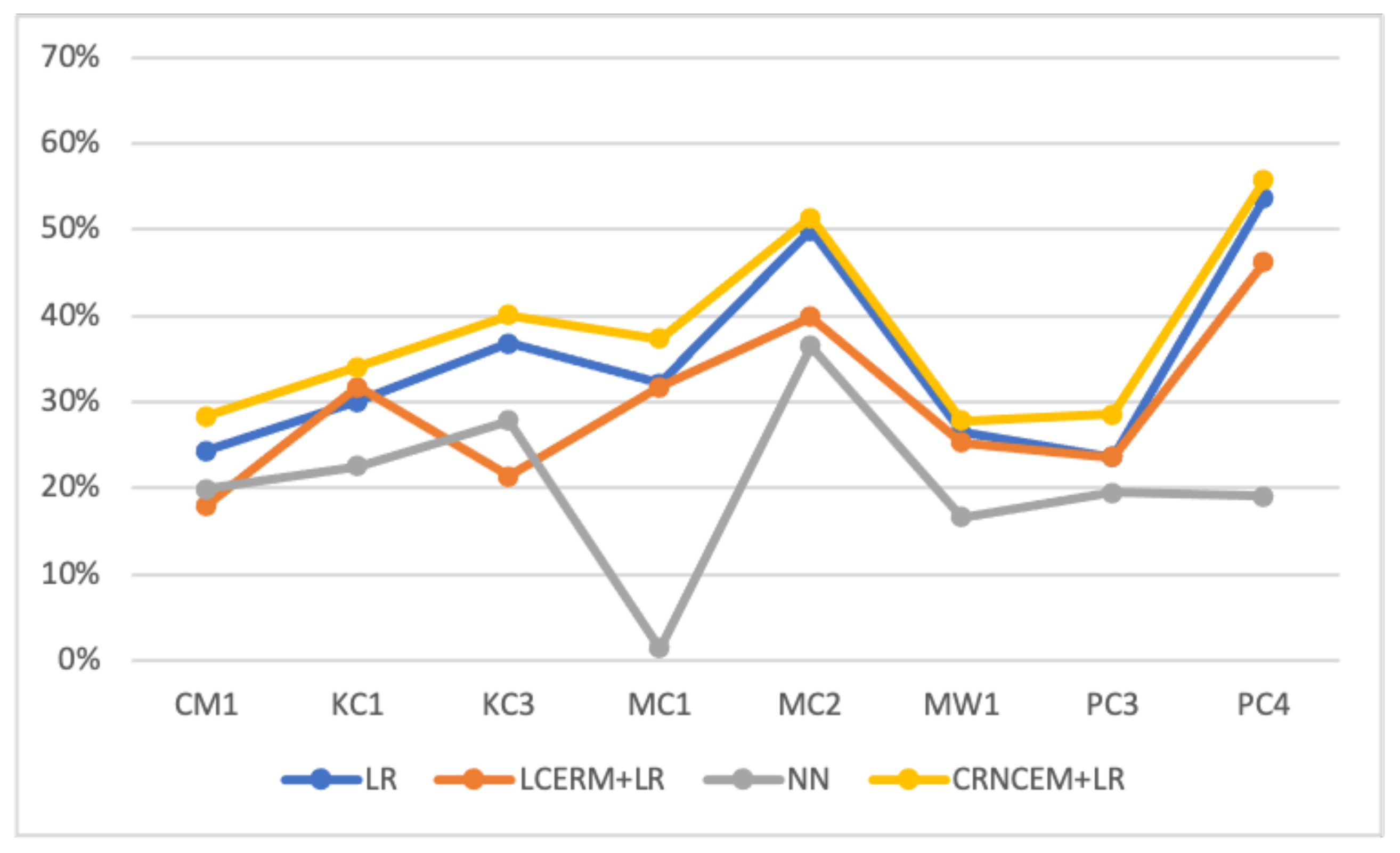
Through extensive experiments, we empirically verified the effectiveness of the proposed CNCERM.

Table 6. Results of CM1.

Dataset	Model	Precision	Recall	F1	Impr F1
CM1	LR	34.3%	20.3%	24.3% *	4.1%
	LCERM + LR	40.9%	13.1%	18.0%
	NN	13.1%	49.2%	19.9%
	CRNCEM + LR	32.7%	26.2%	28.4%

The * indicates the best performance of the compared models.

,

Table 7. Results of KC1.

Dataset	Model	Precision	Recall	F1	Impr F1
KC1	LR	58.4%	20.5%	30.1%	2.3%
	LCERM + LR	60.0%	21.7%	31.8% *
	NN	14.0%	59.2%	22.6%
	CRNCEM + LR	62.8%	23.6%	34.1%

The * indicates the best performance of the compared models.

,

Table 8. Results of KC3.

Dataset	Model	Precision	Recall	F1	Impr F1
KC3	LR	49.6%	31.4%	36.8% *	3.3%
	LCERM + LR	65.1%	14.5%	21.4%
	NN	19.2%	43.6%	27.8%
	CRNCEM + LR	49.5%	35.5%	40.1%

The * indicates the best performance of the compared models.

,

Table 9. Results of MC1.

Dataset	Model	Precision	Recall	F1	Impr F1
MC1	LR	58.6%	22.6%	32.2% *	5.2%
	LCERM + LR	57.4%	23.1%	31.8%
	NN	0.7%	62.1%	1.4%
	CRNCEM + LR	63.7%	27.4%	37.4%

The * indicates the best performance of the compared models.

,

Table 10. Results of MC2.

Dataset	Model	Precision	Recall	F1	Impr F1
MC2	LR	51.4%	49.6%	49.9% *	1.5%
	LCERM + LR	57.3%	31.8%	39.9%
	NN	31.9%	47.9%	36.5%
	CRNCEM + LR	51.9%	51.8%	51.4%

The * indicates the best performance of the compared models.

,

Table 11. Results of MW1.

Dataset	Model	Precision	Recall	F1	Impr F1
MW1	LR	43.0%	21.1%	26.5% *	1.3%
	LCERM + LR	47.1%	18.9%	25.3%
	NN	10.1%	50.0%	16.6%
	CRNCEM + LR	48.5%	22.2%	27.8%

The * indicates the best performance of the compared models.

,

Table 12. Results of PC3.

Dataset	Model	Precision	Recall	F1	Impr F1
PC3	LR	48.0%	16.4%	23.6% *	5.0%
	LCERM + LR	46.3%	16.3%	23.6%*
	NN	12.4%	50.1%	19.5%
	CRNCEM + LR	48.7%	21.0%	28.6%

The * indicates the best performance of the compared models.

and

Table 13. Results of PC4.

Dataset	Model	Precision	Recall	F1	Impr F1
PC4	LR	74.3%	42.2%	53.6% *	2.1%
	LCERM + LR	71.7%	34.5%	46.2%
	NN	12.3%	44.6%	19.1%
	CRNCEM + LR	72.9%	45.6%	55.7%

The * indicates the best performance of the compared models.

show the experimental results, concluding precision rate, recall rate, F1 score, and improved F1 score. Figure 3, Figure 4 and Figure 5 intuitively present each model’s performance.

We have the following observations and analysis:

(1)

Our proposed CNCERM can effectively improve the performance of the LR model. Compared with that of LR, the F1 value of CNCERM+LR improved by 4.1% in CM1, 4.0% in KC1, 3.3% in KC3, 5.2% in MC1, 1.5% in MC2, 1.3% in MW1, 5.0% in PC3, and 2.1% in PC4, with an average of 3.3%. Compared with the best performance of LR and LCERM + LR (indicated by * in Table 6, Table 7, Table 8, Table 9, Table 10, Table 11, Table 12 and Table 13), the F1 value of CNCERM + LR increases by 4.1% in CM1, 2.3% in KC1, 3.3% in KC3, 5.2% in MC1, 1.5% in MC2, 1.3% in MW1, 5.0% in PC3, 2.1% in PC4, with an average 3.1%. Among all three prediction models with LR as the classifier, CNCERM + LR performs best.

(2)

CNCERM + LR performs better than LR, shown in Figure 3, which verifies that the confounding effects of the size metric do affect the prediction performance of LR. The proposed CNCERM can effectively quantify the confounding effects of the class metric and then analyze the direction of the confounding effects. After removing the negative confounding effects, LR significantly improves.

(3)

LCERM + LR performs worse than LR in general, as shown in Figure 3, which means that the traditional confounding removal method is unsuitable for software defect prediction and an inappropriate removal method cannot improve the LR’s performance. Moreover, removing the confounding effects of size metric is not necessarily beneficial to software defect prediction. We should only remove the negative confounding effects that are not conducive to defect prediction.

(4)

Figure 3 intuitively shows that CNCERM + LR performs better than LCERM + LR, indicating that our proposed CNCERM is more suitable for software defect prediction than the linear-based confounding removal method. The predictive ability of LCERM+LR is worse than that of LR, and the predictive ability of CNCERM + LR is stronger than that of LR. The existing confounding removal methods are not suitable for software defect prediction, which further illustrates the necessity of this article.

(5)

Figure 4 intuitively shows that CNCERM + LR and LR have similar precision rates, and each has wins and losses but not much difference. Figure 5 shows that CNCERM + LR has slightly better recall performance than that of LR. These points are why CNCERM + LR has better F1 values; that is to say, C can effectively increase the recall rate of LR, thereby increasing the F1 value of the model.

(6)

We compare CNCERM + LR and NN, and CNCERM+LR has more significant F1 values than that of NN, as shown in Figure 3. By analyzing Figure 4 and Figure 5, we know that the NN model does not perform well in the precision rate, but it performs smoothly in the recall rate and generally has a better performance than that of the CNCERM + LR. The F1 value can comprehensively consider the precision and recall rates. Based on the F1 values, we can conclude that CNCERM + LR has a better predictive ability than that of NN.

5. Conclusions

This paper focuses on a seldom studied but critical issue: removing a size metric’s confounding effects to improve the prediction model’s performance. The confounding effects bring biases into the prediction results. We propose a method named Causally Removing Negative Confound Effects Method (CNCERM) that could remove the negative confounding effects of size metric. First, we quantify the confounding effects of the size metric, then we analyze the directions of the confounding effects, and finally, we selectively remove the negative confounding effects from all. Extensive experimental results verify the effectiveness of CNCERM. Compared with that of Logistic Regression (LR), Linear Confounding Effect Removal Method (LCERM) + LR, and Neural Network (NN), CNCERM + LR achieves the best performance on the F1 in eight NASA data sets.

References

- Kitchenham, B.; Pfleeger, S.L. Software quality: The elusive target [special issues section]. IEEE Softw. 1996, 13, 12–21. [Google Scholar] [CrossRef] [Green Version]
- Gruhn, V. Validation and verification of software process models. In European Symposium on Software Development Environments; Springer: Berlin/Heidelberg, Germany, 1991; pp. 271–286. [Google Scholar]
- Wahono, R.S. A systematic literature review of software defect prediction. J. Softw. Eng. 2015, 1, 1–16. [Google Scholar]
- Catal, C.; Diri, B. A systematic review of software fault prediction studies. Expert Syst. Appl. 2009, 36, 7346–7354. [Google Scholar] [CrossRef]
- Catal, C. Software fault prediction: A literature review and current trends. Expert Syst. Appl. 2011, 38, 4626–4636. [Google Scholar] [CrossRef]
- Radjenović, D.; Heričko, M.; Torkar, R.; Živkovixcx, A. Software fault prediction metrics: A systematic literature review. Inf. Softw. Technol. 2013, 55, 1397–1418. [Google Scholar] [CrossRef]
- Malhotra, R. A systematic review of machine learning techniques for software fault prediction. Appl. Soft Comput. 2015, 27, 504–518. [Google Scholar] [CrossRef]
- Pandey, S.K.; Mishra, R.B.; Tripathi, A.K. Machine learning based methods for software fault prediction: A survey. Expert Syst. Appl. 2021, 172, 114595. [Google Scholar] [CrossRef]
- Yu, C.; Ding, Z.; Chen, X. Hope: Software defect prediction model construction method via homomorphic encryption. IEEE Access 2021, 9, 69405–69417. [Google Scholar] [CrossRef]
- Can, H.; Jianchun, X.; Ruide, Z.; Juelong, L.; Qiliang, Y.; Liqiang, X. A new model for software defect prediction using particle swarm optimization and support vector machine. In Proceedings of the 2013 25th Chinese Control and Decision Conference (CCDC), Guiyang, China, 25–27 May 2013; pp. 4106–4110. [Google Scholar]
- Li, J.; He, P.; Zhu, J.; Lyu, M.R. Software defect prediction via convolutional neural network. In Proceedings of the 2017 IEEE International Conference on Software Quality, Reliability and Security (QRS), Prague, Czech Republic, 25–29 July 2017; pp. 318–328. [Google Scholar]
- Zhu, K.; Zhang, N.; Ying, S.; Wang, X. Within-project and cross-project software defect prediction based on improved transfer naive bayes algorithm. Comput. Mater. Contin. 2020, 63, 891–910. [Google Scholar]
- Heckman, J.J. Sample selection bias as a specification error. Econom. J. Econom. Soc. 1979, 47, 153–161. [Google Scholar] [CrossRef]
- Huang, J.; Gretton, A.; Borgwardt, K.; Schölkopf, B.; Smola, A. Correcting sample selection bias by unlabeled data. Adv. Neural Inf. Process. Syst. 2006, 19, 601–608. [Google Scholar]
- Emam, K.E.; Benlarbi, S.; Goel, N.; Rai, S.N. The confounding effect of class size on the validity of object-oriented metrics. IEEE Trans. Softw. Eng. 2001, 27, 630–650. [Google Scholar] [CrossRef]
- Zhou, Y.; Leung, H.; Xu, B. Examining the potentially confounding effect of class size on the associations between object-oriented metrics and change-proneness. IEEE Trans. Softw. Eng. 2009, 35, 607–623. [Google Scholar] [CrossRef]
- Zhou, Y.; Xu, B.; Leung, H.; Chen, L. An in-depth study of the potentially confounding effect of class size in fault prediction. ACM Trans. Softw. Eng. Methodol. 2014, 23, 1–51. [Google Scholar] [CrossRef]
- Helmert, M. A planning heuristic based on causal graph analysis. In Proceedings of the Fourteenth International Conference on Automated Planning and Scheduling (ICAPS 2004), Whistler, BC, Canada, 3–7 June 2004. [Google Scholar]
- Hastie, T.; Tibshirani, R. Generalized additive models: Some applications. J. Am. Stat. Assoc. 1987, 82, 371–386. [Google Scholar] [CrossRef]
- Tessema, H.D.; Abebe, S.L. Enhancing just-in-time defect prediction using change request-based metrics. In Proceedings of the 2021 IEEE International Conference on Software Analysis, Evolution and Reengineering (SANER), Honolulu, HI, USA, 9–12 March 2021; pp. 511–515. [Google Scholar]
- Eivazpour, Z.; Keyvanpour, M.R. Cssg: A cost-sensitive stacked generalization approach for software defect prediction. Softw. Testing Verif. Reliab. 2021, 31, e1761. [Google Scholar] [CrossRef]
- Bahaweres, R.B.; Suroso, A.I.; Hutomo, A.W.; Solihin, I.P.; Hermadi, I.; Arkeman, Y. Tackling feature selection problems with genetic algorithms in software defect prediction for optimization. In Proceedings of the 2020 International Conference on Informatics, Multimedia, Cyber and Information System (ICIMCIS), Jakarta, Indonesia, 19–20 November 2020; pp. 64–69. [Google Scholar]
- Hall, T.; Beecham, S.; Bowes, D.; Gray, D.; Counsell, S. A systematic literature review on fault prediction performance in software engineering. IEEE Trans. Softw. Eng. 2011, 38, 1276–1304. [Google Scholar] [CrossRef]
- Singh, Y.; Kaur, A.; Malhotra, R. Empirical validation of object-oriented metrics for predicting fault proneness models. Softw. Qual. J. 2010, 18, 3–35. [Google Scholar] [CrossRef]
- Shatnawi, R.; Li, W. The effectiveness of software metrics in identifying error-prone classes in post-release software evolution process. J. Syst. Softw. 2008, 81, 1868–1882. [Google Scholar] [CrossRef]
- Basili, V.R.; Briand, L.C.; Melo, W.L. A validation of object-oriented design metrics as quality indicators. IEEE Trans. Softw. Eng. 1996, 22, 751–761. [Google Scholar] [CrossRef] [Green Version]
- Emam, K.E.; Melo, W.; Machado, J.C. The prediction of faulty classes using object-oriented design metrics. J. Syst. Softw. 2001, 56, 63–75. [Google Scholar] [CrossRef] [Green Version]
- Olague, H.M.; Etzkorn, L.H.; Gholston, S.; Quattlebaum, S. Empirical validation of three software metrics suites to predict fault-proneness of object-oriented classes developed using highly iterative or agile software development processes. IEEE Trans. Softw. Eng. 2007, 33, 402–419. [Google Scholar] [CrossRef]
- Andersson, C.; Runeson, P. A replicated quantitative analysis of fault distributions in complex software systems. IEEE Trans. Softw. Eng. 2007, 33, 273–286. [Google Scholar] [CrossRef]
- MacKinnon, D.P.; Krull, J.L.; Lockwood, C.M. Equivalence of the mediation, confounding and suppression effect. Prev. Sci. 2000, 1, 173–181. [Google Scholar] [CrossRef] [PubMed]
- Fitzmaurice, G. Confused by confounding? Nutrition 2003, 19, 189. [Google Scholar] [CrossRef]
- Catal, C.; Diri, B. Investigating the effect of dataset size, metrics sets, and feature selection techniques on software fault prediction problem. Inf. Sci. 2009, 179, 1040–1058. [Google Scholar] [CrossRef]
- Dickinson, W.; Leon, D.; Fodgurski, A. Finding failures by cluster analysis of execution profiles. In Proceedings of the 23rd International Conference on Software Engineering, Toronto, ON, Canada, 19 May 2001; pp. 339–348. [Google Scholar]
Figure 1.
Path diagram illustrating confounding effect.
Figure 2.
Results of analysis of confounding effects.
Figure 3.
F1 values of four models on eight data sets.
Figure 4.
Precision rates of four models on eight data sets.
Figure 5.
Recall rates of four models on eight data sets.