
Multi-Robot Robust Motion Planning based on Model Predictive Priority Contouring Control with Double-Layer Corridors


School of Automation, Central South University, Changsha 410083, China
*
Author to whom correspondence should be addressed.
Appl. Sci. 2022, 12(3), 1682; https://0-doi-org.brum.beds.ac.uk/10.3390/app12031682
Submission received: 2 December 2021
/
Revised: 30 January 2022
/
Accepted: 3 February 2022
/
Published: 6 February 2022
(This article belongs to the Topic Motion Planning and Control for Robotics)
Abstract
:Featured Application
This work is used for multi-robot autonomous systems.
Abstract
Disturbance poses a major challenge for the safety and real-time performance of robust robot motion planning. To address the disturbance while improving the real-time performance of multi-robot robust motion planning, a model predictive priority contouring control method is proposed. First, an improved conflict-based search (ICBS) planner is utilized to plan reference paths. The low-level planner of the conflicted-based search (CBS) planner is replaced by the hybrid A* planner and reference paths are adopted as an initial guess of model predictive priority contouring control. Second, double-layer corridors are proposed to provide safety guarantees, which include static-layer corridors and dynamic-layer corridors. The static-layer corridors are generated based on reference paths and the dynamic-layer corridors are generated based on the relative positions and velocities of robots. The double-layer corridors are applied as safety constraints of model predictive priority contouring control. Third, a prioritization mechanism is devised to improve computational efficiency. Priorities are assigned according to each robot’s task completion percentage. Based on the assigned priority, multiple robots are grouped, and each group executes the model predictive priority contouring control algorithm to acquire trajectories. Finally, our method is compared with the centralized method and the soft constraint-based DMPC. Simulations verify the effectiveness and real-time performance of our approach.
1. Introduction
Multi-robot systems play a vital role in next-generation factories, urban search and rescue, and package delivery, and they are anticipated to be applied in space exploration [1,2]. One of the key ingredients to a multi-robot system is the motion planning module. The motion planning module should find a set sequence of valid configurations that move multiple robots from starting points to goal points safely [3]. However, in unstructured environments, the multi-robot motion planning algorithm being both optimal, complete, real-time, and flexible is still a valuable and challenging problem to be solved, especially in the presence of disturbances.
As mentioned in previous publications, the multi-robot motion planning (MMP) problem is generally defined as a multi-objective optimization problem with different types of constraints [4,5]. The methods for solving MMP problems are mainly classified into centralized and decentralized methods [3].
Centralized methods plan the motion trajectories of robots jointly [6]. In [7], Guni Sharon et al. proposed a two-level algorithm called conflict-based search (CBS) to find optimal paths for multiple robots. The core of the algorithm is to maintain a constraint tree to resolve conflicts and plan the optimal path for each robot with constraints. In [8], Jiaoyang Li et al. improved the CBS algorithm based on explicit estimation search. Their method utilizes online learning to acquire the unacceptable estimated cost of the solution and adopts explicit estimation search to resolve conflicts. Although these methods guarantee optimality and real-time performance, the paths are discrete nodes and the application is limited to holonomic robots. Since the above methods do not consider the robot kinematic and dynamical characteristics, the paths generally need to be further processed before they can be applied to non-holonomic robots.
To deal with the MMP problem of non-holonomic robots, a two-stage pipeline, i.e., reference path planning and trajectory generation, is applied in a series of works [9,10,11]. In these works, collision-free paths are planned for all robots firstly. Then, the reference paths are treated as an initial guess of the MMP problem. The nonlinear optimization problem [11] or quadratic problem [9,10] is formulated to obtain collision-free dynamically feasible trajectories. Compared with solving the problem without an initial guess, the two-stage pipeline can achieve better efficiency and quality.
Decentralized methods typically decouple large-scale multi-robot motion planning problems into multiple smaller-scale multi-robot motion planning problems [6]. The most famous decentralized method is the velocity obstacle method [12,13,14,15]. The main idea of the velocity obstacle method is to choose a suitable velocity in the feasible velocity set. As this method only considers local obstacle avoidance, the global performance is poor and may lead the robot into deadlock. Another well-known decentralized method is distributed model predictive control (DMPC) [4,16,17]. In [17], Luis et al. proposed a distributed model predictive control (DMPC) method for multi-robot motion planning to generate trajectories in real-time. The DMPC method improves computational efficiency but reduces the quality of the solution.
More importantly, multi-robot systems operating in the real world are often subject to various disturbances. Disturbances lead to inaccurate estimates of the states of multi-robot systems. To ensure robustness in multi-robot motion planning, disturbances need to be considered in the design of the algorithm. The disturbances are often modeled as chance constraints [18,19,20]. In [21], Wenhao Luo et al. defined a chance constraint called probabilistic safety barrier certificates (PrSBC) and solved an optimization problem with the PrSBC. In [22], Bharath Gopalakrishnan et al. studied a probabilistic variant of the reciprocal velocity obstacle method called probabilistic reciprocal velocity obstacle (PRVO). This approach converts the disturbances into chance constraints on the velocity. In [23], Hai Zhu et al. designed a tight bound on the collision probability approximation and presented a nonlinear model predictive control method to obtain trajectories of each robot.
Considering the above factors, a model predictive priority contouring control method is proposed. First, the reference paths are generated by the ICBS planner. The low-level planner of the CBS planner is replaced by the hybrid A* planner. The reference paths are utilized as the initial guess of model predictive priority contouring control. Second, double-layer corridors are devised to provide robust safety guarantees. The static-layer corridors are generated based on reference paths and the dynamic-layer corridors are generated based on relative positions and velocities of robots. The double-layer corridors are applied as safety constraints of model predictive priority contouring control. Third, a prioritization mechanism is proposed to improve the computational efficiency of model predictive priority contouring control. The key contributions of this paper are as follows.
- The construction method of double-layer corridors is devised, and the chance constraints introduced by disturbances are transformed into linear deterministic safety constraints.
- Model predictive priority contouring control with the double-layer corridors is proposed to generate multi-robot trajectories, which ensures security while greatly improving computational efficiency.
- Extensive evaluation of the method through a great number of simulations.
The rest of the paper is organized as follows. In Section 2, the problem of multi-robot robust motion planning is stated. In Section 3, double-layer corridors are devised. In Section 4, the model predictive priority contouring control with double-layer corridors is proposed. In Section 5, simulations are present. Finally, Section 6 concludes our work.
2. Problem Statement of Multi-Robot Robust Motion Planning
The purpose of multi-robot robust motion planning is to ensure the safety of multi-robot motion planning even disturbed. Suppose that there are N mobile robots in the environment. The mobile robots may have different sizes d, different maximum velocity max, maximum acceleration max, maximum angular velocity max, and maximum angular acceleration max.
2.1. Robot Model
In this paper, differential wheeled robots are studied. The planning process is carried out in the SE(2) space and state xm,k includes 2-D position (xm,k, ym,k) and orientation . The robot model f(·) can be written as Equation (1).
In Equation (1), m,k and m,k are the velocity and angular velocity of robot m at time k respectively. represents the time interval between two control inputs. Based on the robot model (1), the control input of robot m at time k is defined as um,k = [vm,k, wm,k].
It is worth mentioning that Equation (1) is the ideal kinematic model of the robot. Under pure rolling conditions, the motion of the robot is exactly in accordance with Equation (1). However, imperfections are unavoidable in real devices [24]. Complex wheel-ground interactions and system noises cause disturbances to the robots. Moreover, these disturbances are modeled as Gaussian random variables, characterized by their mean and covariance matrices. Thus, the model of a given robot m at time k are defined as Equation (2).
In Equation (2), and are the state and control input of robot m at the time k respectively. is an unknown disturbance with Gaussian probability distribution. Considering the disturbance level in the real environment, is set to . What is more, the simulations are carried out under different level disturbances. Related simulations are in Section 5.1.
2.2. Collision Avoidance
The workspace of the robot is defined as . Let denote the position of robot m and denote the position of obstacle o. Hence, the collision condition of robot m with obstacle o at time k is given as follows.
In Equation (3), dm represents the minimum safe distance of robot m.
For any two robots m and n, if their position and satisfy the following equation
there is a collision between robot m and n.
Due to the disturbances, the position of the robot is a Gaussian random variable. Chance safety constraints are given as Equations (5) and (6).
In Equation (5), is the probability threshold for robot-obstacle collision. In Equation (6), is the probability threshold for inter-robot collision
2.3. Multi-Robot Robust Motion Planning Problem
The multi-robot motion planning (MMP) problem is generally defined as a multi-objective optimization problem with different types of constraints [4,5]. Thus, the general form of multi-robot robust motion planning is modeled as a multi-objective optimization problem in this paper. Section 2.1 shows the robot model constraint, and Section 2.2 gives safety constraints. What is more, the control input of each robot is constrained by its maximum velocity, maximum acceleration, maximum angular velocity, and maximum angular acceleration. Meanwhile, the position and yaw at the initial time constrain the initial state of each robot. Based on the above discussion, the multi-robot robust motion planning problem can be defined as follows.
In Equation (7), . Equation (7a) is the cost function. In this paper, we define J as a cost function that forces the robot to stay near the reference path and track it synchronously. The exact form is given in Section 4.3.3. In Equation (7a), and . The kinematic model of the robots with disturbances is presented as Equation (7b). Equations (7c,d) model the safety constraints. Equations (7e,f) provide control input constraints. The initial state constraint is denoted by Equation (7g).
The key difficulty in solving this problem is how to deal with the safety constraints (7c,d). The safety constraints (7c,d) are nonconvex constraints represented by the integral of a multivariate Gaussian distribution. These types of constraints are called chance constraints. They are intractable to handle in the usual case. To make the problem easy to solve, double-layer corridors are devised. Then, the problem can be transformed into a deterministic optimization problem.
3. Double-Layer Corridor
In this section, double-layer corridors are proposed to provide safety guarantees. Double-layer corridors include static-layer corridors and dynamic-layer corridors. Static-layer corridors ensure obstacle collision avoidance and dynamic-layer corridors ensure inter-robot collision avoidance.
3.1. Static-Layer Corridor
A series of partially overlapping convex sets are often used to model the safe region of robots to minimize the number of collision avoidance constraints [11]. These convex sets are defined as static-layer corridors in this paper. The collision avoidance between robot and obstacle is guaranteed by static-layer corridors.
To construct static-layer corridors, the minimum safe distance between the robot and the obstacle needs to be obtained. Assume that the position of the robot m at time k is a multivariate Gaussian random variable and obstacle o is located at . Then, is also a Gaussian random variable, i.e., . Thus, the collision probability is given by Equation (8).
Equation (8) is the integral over the circle of the multivariate Gaussian probability density function. Referring to [25], the circle collision region mo,k is enlarged into a half space mo,k′. mo,k′ is defined as Equation (9).
In Equation (9), . Since , Equation (10) can be obtained.
Lemma 1.
Letbe a multivariate Gaussian random variable. Then,
Lemma 2.
Letbe a multivariate Gaussian random variable and a probability threshold. There is a deterministic equivalent form to
which is shown as Equation (14).
Based on Lemma 1, Equation (10) can be rewritten as follows.
After that, according to Lemma 2, Equation (16) can be acquired
According to Equation (16), the minimum safe distance between the robot and the obstacle can be obtained in real-time.
A series of partially overlapping convex sets are utilized to model the safe region of robots. The series of partially overlapping convex sets are defined as static-layer corridors . For robot m, the static-layer corridors are shown in Figure 1. Each yellow rectangle represents a static-layer corridor. They model an obstacle-free area for the robot m.
For the kth static-layer corridor of robot m, it satisfies Equation (17) and Equation (18).
Equation (17) guarantees that the intersection of the kth static-layer corridor and the obstacle region is empty. Moreover, Equation (18) enforces that the kth static-layer corridor and the static-layer corridor are sequentially connected.
The distance between the boundary of a static-layer corridor and the obstacle is set as , which is shown in Figure 2. is set to an initial value at the beginning and updates during the robot’s operation.
In Equation (19), represents the generalized inverse matrix of . In Equation (20), is the position of point M and is the position of point N. M is a point on the boundary of static-layer corridor and N is its vertical point on the obstacle area. If robot m stays inside the static-layer corridor, then Equation (16) satisfies. When the robot satisfies Equation (16), the robot cannot collide with the obstacle.
Thus, it can be seen that if the state of robot m satisfies Equation (21), there is no obstacle collision.
3.2. Dynamic-Layer Corridor
Collision avoidance between robots is ensured by dynamic-layer corridors. Similar to the static-layer corridor, the minimum safe distance between the robots needs to be obtained.
Let the position of the robot m and n be multivariate Gaussian random variables , . Then is also a Gaussian random variable, i.e., . The collision probability is given by Equation (22).
Similarly, according to Lemma 1 and Lemma 2, Equation (23) can be acquired.
In Equation (23), and .
The minimum safe distance between robot m and robot n is acquired based on Equation (23). However, ignoring the velocity of the robots may result in the collision avoidance condition (23) not being satisfactory. Generally, the problem is addressed by the velocity obstacle method [12,13,14,15]. However, the constraint obtained by the velocity obstacle method is nonconvex. Jungwon Park et al. adopted the constant velocity assumption to predict short trajectories of robots and simplified the constraint by ensuring that the predicted trajectories do not collide [26]. Therefore, let m and n be the velocities of robot m and robot n, respectively. After a very short time , the position of robot m is , , and the position of robot n is , . , which is needed to satisfy Equation (24).
In Equation (24), .
In this paper, the set is defined as the dynamic-layer corridor for robot m and robot n. The set satisfies Equation (25).
Equation (25) guarantees that the intersection of the dynamic-layer corridor and the inter-collision region of robot m and robot n is empty. For any robot m, it can be seen that if the state of robot m satisfies Equation (26), there is no collision between robot m and robot n.
4. Model Predictive Priority Contouring Control with Double-Layer Corridors
The model predictive priority contouring control with double-layer corridors is proposed in this section. The whole framework is shown in Figure 3. First of all, reference path planning is performed using the ICBS planner. The reference paths are adopted as an initial guess of model predictive priority contouring control. Then, the construction process of double-layer corridors is described in detail. The double-layer corridors are applied as safety constraints of model predictive priority contouring control. At last, a prioritization mechanism is devised to improve the computational efficiency of model predictive contouring control. The improved algorithm is defined as model predictive priority contouring control.
4.1. Reference Path Planning
The multi-robot motion planning with disturbances is nonlinear, nonconvex, and NP-hard. It is difficult to obtain the solution in real-time. Thus, the ICBS planner is adopted to find discrete and collision-free reference paths for multiple robots. The solution is regarded as an initial guess for the multi-robot motion planning with disturbances. A more accurate solution is acquired by the method proposed in Section 4.3.4.
In this paper, the environment is modeled by a voxel grid map, and each grid has eight neighbors. Thus, the whole map can be regarded as an undirected graph G = {V, E}. The vertex ∈V is the free grid of the map and the edge (i,j) represents that the gird j is a neighbor of the grid i. The ICBS planner works in two levels. At the high level, the constraint tree is built to resolve potential conflicts. At the low level, the hybrid A* planner is utilized to replace the A* planner. The kinematics of the robot is considered during the planning process and discrete paths are planned for robots with the constraints of the constraint tree. The procedure is as follows.
First, the hybrid A* planner searches paths for each robot with no constraints. Second, the constraint tree checks for conflicts between the paths of every two robots. Referring to [7], two types of conflicts are applied when planning reference paths. The first one is a vertex conflict. If robot m and robot n occupy the same grid at time k, vertex conflict occurs. This kind of conflict is defined by Equation (27). The second type of conflict is edge conflict. If robot n moves from i to j and robot m moves from j to i between time k and k+1, there is an edge conflict (28).
Third, assuming a conflict arises, two nodes will be added to the constraint tree. The first one adds constraint for robot m to avoid the collision. The second node adds constraint for robot n to avoid the collision. Fourth, each time a new node is generated in the constraint tree, the hybrid A* planner re-plans the path for the robot with the new constraint. Finally, repeat the above process until all reference paths are planned.
4.2. Construction of Double-Layer Corridor
4.2.1. Construction of Static-Layer Corridor
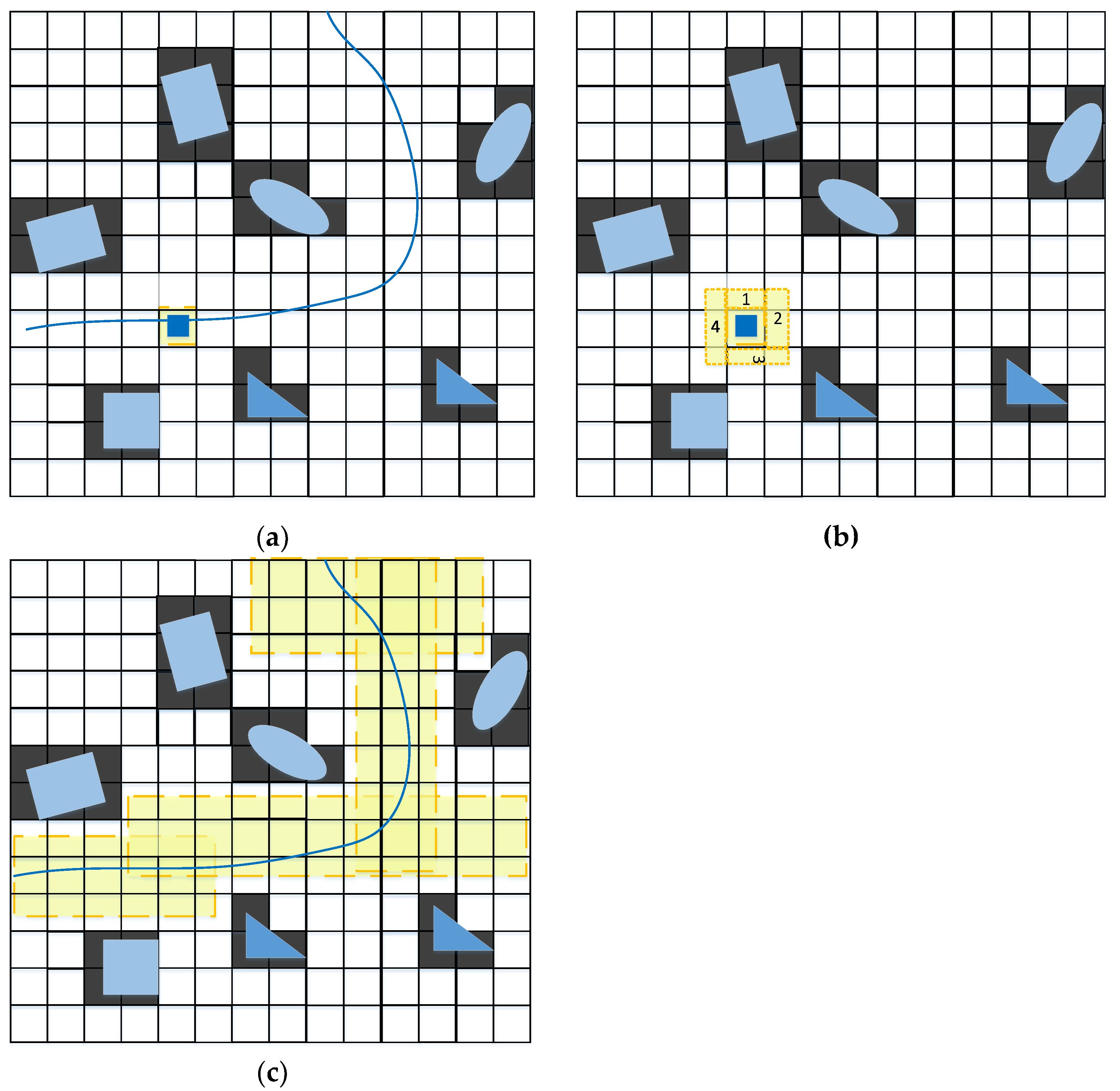
The goal for the construction of the static-layer corridors of robot m is to find a group of free convex polygons to take up as much free workspace as possible. Since the environment is modeled by a voxel grid map, is a convex hull of free voxel grids. The static-layer corridors are constructed by an axis-search method. The procedure is shown in Figure 4.
In Figure 4, black grids represent the obstacle region. The blue curve is the reference path of robot m. As Figure 4a shows, the static-layer corridor is initialized by a grid in the reference path. The grid is marked by a blue square. Each static-layer corridor expands to the maximum axis-aligned area. These static-layer corridors are represented by the yellow rectangle in Figure 4b. The steps to construct static-layer corridors are as follows.
To begin with, the grids occupied by the reference path points are applied to initialize the static-layer corridors. Next, static-layer corridors expand step by step in all axis-aligned directions until they cover the maximum free workspace. Further, the duplicated static-layer corridors are checked. Static-layer corridors occupying exactly the same area are reserved for only one. Complete the above process for each robot. Finally, the boundaries of the static-layer corridors are updated based on Equation (19) while the multi-robot system is running.
4.2.2. Construction of Dynamic-Layer Corridor
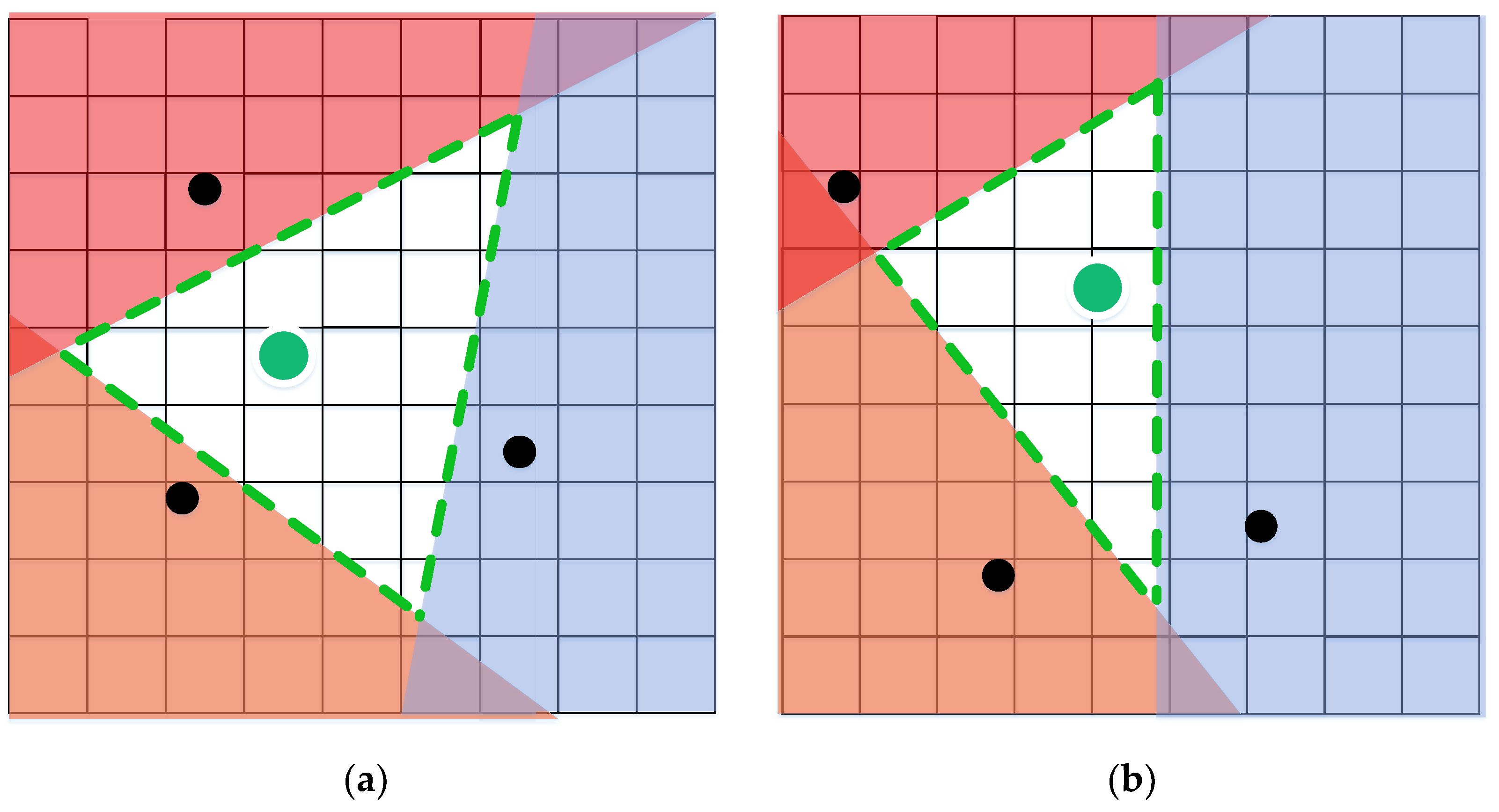
The purpose of constructing dynamic corridors is to avoid collisions between robots. The construction process of the dynamic-layer corridor is shown in Figure 5.
In Figure 5, the green circle represents robot m and the convex area marked with green dotted lines is the dynamic-layer corridor of robot m. For robot m, it treats other robots as obstacles with velocity. Other robots are indicated by black circles in Figure 5. For robot m, it cannot collide with robots that are too far away. To reduce the consumption of computing resources, reciprocal avoidance distance L is introduced. For any two robots m and n, if their relative distance , then ignores the dynamic-layer corridor construction between them. The steps to construct dynamic-layer corridors are as follows.
Firstly, calculate their relative distances for any robot m and n. Secondly, construct dynamic-layer corridors for robots whose relative distance is less than L. Finally, the boundaries of the dynamic-layer corridors are updated based on Equation (25) while the multi-robot system is running.
4.3. Model Predictive Priority Contouring Control
A prioritization mechanism is devised to improve the computational efficiency of model predictive contouring control. The improved algorithm is defined as model predictive priority contouring control. What is more, the reference paths are processed as the initial guess and double-layer corridors are employed as safety constraints.
4.3.1. Initial Guess
Let denote the reference path point of robot m. Processing is carried out here to obtain an initial guess for yaw, velocity, and angular velocity.
In Equation (29), is the reference yaw of robot m. In Equation (30), is the reference velocity of robot m and denotes the time interval between two control signals. In Equation (31), is the reference angular velocity of robot m.
4.3.2. Constraints
To obtain safe dynamically feasible trajectories, the proposed method should satisfy robot dynamic constraints, kinematic constraints, and safety constraints.
The dynamic constraints and kinematic constraints of the robot include robot model constraints, state constraints, and control input constraints. The robot model constraint is shown as Equation (2). The state constraints and control input constraints are shown as Equation (7e,f). The safety constraints (7c,d) are nonlinear nonconvex chance constraints. In Section 3, static-layer corridors and dynamic-layer corridors are proposed to ensure safety. Static-layer corridors provide obstacle avoidance guarantees and dynamic-layer corridors provide inter-robot collision avoidance guarantees. Thus, safety constraints (7c,d) are transformed into static-layer corridors constraints (21) and dynamic-layer corridors constraints (26).
4.3.3. Cost Function
The design of the cost function is particularly important to ensure the smooth operation of multi-robot systems. The cost function constructed in this paper mainly includes the deviation term and the input smoothing term.
In Equation (32), l1, l2, and l3 are weight factors. a is the cost of deviating from the reference paths. ensures smooth velocity changes and ensures smooth angular velocity changes.
Referring to [27], the cost is defined as the sum of contour error and lag error . The contour error and the lag error are shown in Figure 6.
In Equation (33), represents the kth trajectory point of robot m. N is the number of robots and K is the number of reference path points.
The input smoothing term and are given as follows.
In Equation (34), m,k is the velocity of robot at time k and represents the time interval between two control signals. In Equation (35), m,k is the angular velocity of robot at time k.
4.3.4. Prioritization Mechanism
Based on the previous discussion, the multi-robot robust motion planning of Section 2 can be rewritten in the following form.
In Equation (36), . Equation (36a) represents the cost function: the details of its items are discussed previously. Equation (36b) is robot model constraints. Equation (36c) is obstacle avoidance constraint. Equation (36d) is inter-collision avoidance constraint. Equation (36e,f) represent control input constraints. The initial state constraints are denoted by Equation (36g).
This paper uses an open-source solver, qpOASES [28], to solve (36). Although the constraints are simplified as much as possible, it is still difficult to solve in real-time for large-scale robotic systems. Therefore, a prioritization mechanism is devised to decouple the problem (36). The schematic diagram is shown in Figure 7. In Figure 7, high-priority robots are indicated by black circles, and they are regarded as obstacles by low-priority robots.
For each robot, the reference path is defined as its task to accomplish. The priority of each robot is constructed in terms of the percentage of uncompleted tasks. Each robot’s reference path points are constructed as a task queue. When a robot travels past a reference path point, it is removed from the queue and the percentage of uncompleted tasks is calculated as follows.
In Equation (37), Pm represents the percentage of tasks that the robot m did not complete. m represents the number of path points left in the task queue of robot m. m, ref represents the initial number of reference path points in the task queue of robot m.
First, let Prank be the result of the robot priority ranking. In the beginning, the priority is assigned according to the robot ID. Second, S robots with the highest priority are selected to form a group according to the priority ranking, and the (36) composed of these S robots are solved using model predictive contouring control. Third, these S robots are removed from the task ranking queue Prank, and the process is repeated until all robot trajectories are acquired. During the solution process, the high-priority robots and their trajectories are treated as obstacles for the low-priority robots. Fourth, the first group control signal in the control sequence is used as input to each robot. Fifth, the priority of the robots is re-assigned according to the value of Equation (37) from the largest to the smallest. Finally, the above process is repeated until all robots reach their goals. The whole process is shown as Algorithm 1.
| Algorithm 1: Model Predictive Priority Contouring Control. |
| Initial guess preprocessing; InitializePrank While not all robots reach the goal While Prank ≠ φ Select S robots with the highest priority in Prank; Solve (36) composed of these S robots Remove those S robots from Prank foreach robot Calculate the percentage of the uncompleted tasks Pm; Append Pm to Prank end Sort Prank end end |
5. Simulation Analysis
The method proposed in this paper is implemented by C++ and runs under the Ubuntu 16.04, ROS kinetic. The computer hardware configuration is Intel i7-9750H 2.60 GHz, 32 GB RAM. In this paper, a grid map is used to represent the whole environment and the environment is an area of 4 m ∗ 4 m. The grid size is set to 0.25 m. The center of the area is set as the coordinate origin. Right is the positive direction of the x-axis and upward is the positive direction of the y-axis. The time interval is 0.2 s. The probability threshold and are both 5%. The safety distance is 0.15m. The maximum velocity max of each robot is 1 m/s, and the maximum angular velocity max is 1 rad/s. The maximum acceleration max of each robot is 2 m/s2, and the maximum angular acceleration max is 1 rad/s2. The prediction horizon length of model predictive priority contouring control is 8. Batch size S is 3.
5.1. Simulation under Different Level Disturbances
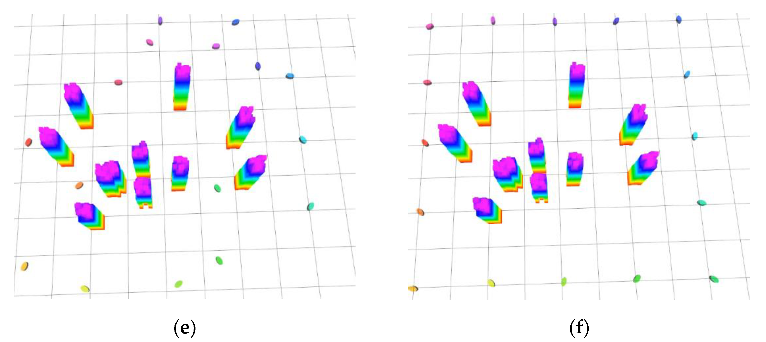
Disturbances include position disturbances and angular disturbances. In this paper, the covariance matrix is used to represent the disturbances. The covariance matrix is set to . The last one represents the angular disturbance and the other two terms are the position disturbances. The starts and goals of the robot are shown in Table 1. The operation of the multi-robot system is shown in Figure 8.
The minimum distance between robot and obstacle and the minimum distance between robots during the operation of the multi-robot system are recorded. The solid line in Figure 9a indicates the minimum distance between obstacle and robot. The solid line in Figure 9b presents the minimum distance between robots. It can be seen that each robot can arrive at the goals safely at the end.
To verify the effectiveness of the proposed method. The simulation is done under different level disturbances. In this paper, the proposed method is evaluated in terms of safety, task success rate, operational efficiency, and computational efficiency. The simulation is done fifteen times under each condition, and the results are shown in Table 2.
In terms of safety, it can be seen from Table 2 that as the level of disturbance increases, the minimum distance between robot and obstacle increases, and the minimum distance between robots increases. Moreover, it can be seen from Figure 9 that there is no collision between robots and no collision between robot and obstacles during the entire operation of the robots. In terms of task success rate, our method achieves a 100% task success rate at various levels of disturbances. In terms of operational efficiency, the average velocity of the multi-robot system decreases, and task time increases as the level of disturbance increases. However, the difference is not very large. In terms of computational efficiency, it can be seen from Table 2 that the difference in computational time consumption is not significant.
5.2. Method Comparison and Analysis
To further verify the effectiveness, our method is compared with the centralized method [6] and the soft constraint-based DMPC method [17].
The starts and goals are the same as in Table 1. Meanwhile, the robot operating environment and parameter settings are the same as in Section 5.1. The covariance matrix is set to . Fifteen independent repeated simulations are carried out. The different methods are evaluated in terms of task success rate, safety, operational efficiency, and computational efficiency. Results are shown in Table 3.
It is important to note that task time refers to the time spent on the mission in the simulation while calculation time refers to the time spent by the CPU in the real world.
In terms of task success rate, our method and centralized method achieve a 100% task success rate. There is a failure when the soft constraint-based DMPC is utilized. The task success rate of soft constraint-based DMPC is 93.3%. Thus, the soft constraint-based DMPC is more sensitive to disturbances and our method is more robust.
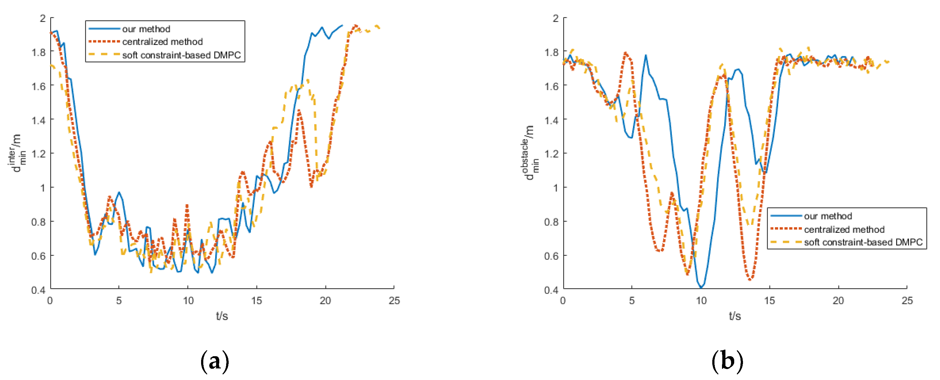
In terms of safety, the successful results of all methods are compared. Figure 10a presents the minimum distance between robots. In addition, Figure 8b illustrates the minimum distance between robot and obstacle. The minimum distance between robot and obstacle for our method, the centralized method, and the soft constraint-based DMPC are 0.40 m, 0.38 m, and 0.40 m, respectively. Moreover, the minimum distances between the robots for our method, the centralized method, and the soft constraint-based DMPC are 0.50 m, 0.51 m, and 0.44 m, respectively.
In terms of operational efficiency, the average velocity of our method is 15% higher than that of the centralized method, and the task time of our method is 6.80% less than that of the centralized method. Moreover, the average velocity of our method is 25% higher than that of the soft constraint-based DMPC, and the task time of our method is 12.1% less than that of the soft constraint-based DMPC.
In terms of computational efficiency, the calculation time per horizon of our method is longer than that of the soft constraint-based DMPC. However, the difference is not significant. Moreover, it can be seen that our method is much more computationally efficient than the centralized method.
5.3. Computational Time Consumption Comparison and Analysis
In this section, the computational performance and the quality of the results of our method are further compared with other methods. Simulations are performed under different numbers of robots. The cost is utilized to evaluate the quality of the results and calculation time per horizon is utilized to evaluate the computational efficiency. Since the soft constraint-based DMPC does not guarantee a 100% success rate, our method is compared with the centralized method. The robot operating environment and parameter settings are the same as in Section 5.1. The covariance matrix is set to . The results are shown in Figure 11.
As can be seen from Figure 11a, the computational efficiency of our method decreases slightly as the number of robots increases while the computational efficiency of the centralized method decreases rapidly. Figure 11b illustrates that the cost of our method is a little higher than that of the centralized method. According to the experimental data, the computational efficiency of our method is on average 3.50 times higher than that of the centralized method, and the cost is on average 23.9% higher than that of the centralized method.
6. Conclusions
A model predictive priority contouring control is proposed to deal with the problem of multi-robot robust motion planning in this paper. Firstly, the ICBS planner is utilized to obtain the initial guess for model predictive priority contouring control. The low-level planner of the CBS planner is replaced by the hybrid A* planner. Second, double-layer corridors are proposed to deal with chance safety constraints. Static-layer corridors ensure obstacle avoidance and dynamic-layer corridors guarantee inter-robot collision avoidance. The double-layer corridors are applied as safety constraints of model predictive priority contouring control. Third, a prioritization mechanism is devised to improve the computational efficiency of model predictive contouring control. The priority of the robot is assigned based on the percentage of uncompleted tasks. Finally, simulations show the effectiveness and real-time performance of our approach in multi-robot robust motion planning. In future work, the authors plan to extend the proposed method to a maze-like environment. Moreover, interaction with unknown dynamic obstacles will be considered in our future work.
Author Contributions
Conceptualization, L.Y.; methodology, L.Y. and Z.W.; software, Z.W.; validation, L.Y.; formal analysis, Z.W.; investigation, Z.W.; resources, Z.W.; data curation, Z.W.; writing—original draft preparation, Z.W.; writing—review and editing, L.Y.; visualization, Z.W.; supervision, L.Y.; project administration, L.Y.; funding acquisition, L.Y. All authors have read and agreed to the published version of the manuscript.
Funding
This work was financially supported by the National Natural Science Foundation of China (No. 61976224, 61976088).
Institutional Review Board Statement
Not applicable.
Informed Consent Statement
Not applicable.
Data Availability Statement
Not applicable.
Conflicts of Interest
The authors declare no conflict of interest.
References
- Chatziparaschis, D.; Michail, G.L.; Partsinevelos, P. Aerial and Ground Robot Collaboration for Autonomous Mapping in Search and Rescue Missions. Drones 2020, 4, 79. [Google Scholar] [CrossRef]
- Choudhury, S.; Gupta, J.K.; Kochenderfer, M.J.; Sadigh, D.; Bohg, J. Dynamic multi-robot task allocation under uncertainty and temporal constraints. Auton. Robot. 2021, 1–17. [Google Scholar] [CrossRef]
- Madridano, Á.; Al-Kaff, A.; Martín, D.; de la Escalera, A. Trajectory planning for multi-robot systems: Methods and applications. Expert Syst. Appl. 2021, 173, 114660. [Google Scholar] [CrossRef]
- Luis, C.E.; Marijan, V.; Schoellig, A.P. Online trajectory generation with distributed model predictive control for multi-robot motion planning. IEEE Robot. Autom. Lett. 2020, 5, 604–611. [Google Scholar] [CrossRef] [Green Version]
- Li, B.; Ouyang, Y.; Zhang, Y.; Acarman, T.; Kong, Q.; Shao, Z. Optimal Cooperative Maneuver Planning for Multiple Nonholonomic Robots in a Tiny Environment via Adaptive-Scaling Constrained Optimization. IEEE Robot. Autom. Lett. 2021, 6, 1511–1518. [Google Scholar] [CrossRef]
- Li, B.; Liu, H.; Xiao, D.; Yu, G.; Zhang, Y. Centralized and optimal motion planning for large-scale AGV systems: A generic approach. Adv. Eng. Softw. 2017, 106, 33–46. [Google Scholar] [CrossRef]
- Sharon, G.; Stern, R.; Felner, A.; Sturtevant, N.R. Conflict-based search for optimal multi-agent pathfinding. Artif. Intell. 2015, 219, 40–66. [Google Scholar] [CrossRef]
- Li, J.; Ruml, W.; Koenig, S. EECBS: A Bounded-Suboptimal Search for Multi-Agent Path Finding. In Proceedings of the 35th AAAI Conference on Artificial Intelligence (AAAI), Online, 2–9 February 2021. [Google Scholar]
- Hönig, W.; Preiss, J.A.; Kumar, T.S.; Sukhatme, G.S.; Ayanian, N. Trajectory planning for quadrotor swarms. IEEE Trans. Robot. 2018, 34, 856–869. [Google Scholar] [CrossRef]
- Debord, M.; Hönig, W.; Ayanian, N. Trajectory planning for heterogeneous robot teams. In Proceedings of the 2018 IEEE/RSJ International Conference on Intelligent Robots and Systems (IROS), Madrid, Spain, 1–5 October 2018. [Google Scholar]
- Li, J.; Ran, M.; Xie, L. Efficient trajectory planning for multiple non-holonomic mobile robots via prioritized trajectory optimization. IEEE Robot. Autom. Lett. 2021, 6, 405–412. [Google Scholar] [CrossRef]
- Wilkie, D.; van den Berg, J.; Manocha, D. Generalized velocity obstacles. In Proceedings of the 2009 IEEE/RSJ International Conference on Intelligent Robots and Systems, St. Louis, MO, USA, 10–15 October 2009. [Google Scholar]
- Van den Berg, J.; Lin, M.; Manocha, D. Reciprocal velocity obstacles for real-time multi-agent navigation. In Proceedings of the 2008 IEEE International Conference on Robotics and Automation, Pasadena, NL, Canada, 19–23 May 2008. [Google Scholar]
- Snape, J.; Van Den Berg, J.; Guy, S.J.; Manocha, D. The hybrid reciprocal velocity obstacle. IEEE Trans. Robot. 2018, 27, 696–706. [Google Scholar] [CrossRef] [Green Version]
- Alonso-Mora, J.; Breitenmoser, A.; Rufli, M.; Beardsley, P.; Siegwart, R. Optimal Reciprocal Collision Avoidance for Multiple Non-Holonomic Robots. In Proceedings of the 10th International Symposium on Distributed Autonomous Robotic Systems, Ecole Polytechn Fed, Lausanne, Lausanne, Switzerland, 1–3 November 2011. [Google Scholar]
- Katriniok, A.; Sopasakis, P.; Schuurmans, M.; Patrinos, P. Nonlinear model predictive control for distributed motion planning in road intersections using PANOC. In Proceedings of the 2019 IEEE 58th Conference on Decision and Control (CDC), Nice, France, 11–13 December 2019. [Google Scholar]
- Luis, C.E.; Schoellig, A.P. Trajectory generation for multiagent point-to-point transitions via distributed model predictive control. IEEE Robot. Autom. Lett. 2019, 4, 375–382. [Google Scholar] [CrossRef] [Green Version]
- Bharath, G.; Singh, A.K.; Kaushik, M.; Krishna, K.M.; Manocha, D. Chance constraint based multi agent navigation under uncertainty. In Proceedings of the Advances in Robotics (AIR 2017), New Delhi, India, 28 June–2 July 2017. [Google Scholar]
- Zhou, L.; Tokekar, P. Multi-robot coordination and planning in uncertain and adversarial environments. Curr. Robot. Rep. 2021, 2, 147–157. [Google Scholar] [CrossRef]
- Ono, M.; Williams, B.C.; Blackmore, L. Probabilistic planning for continuous dynamic systems under bounded risk. J. Artif. Intell. Res. 2013, 46, 511–577. [Google Scholar] [CrossRef]
- Luo, W.; Sun, W.; Kapoor, A. Multi-Robot Collision Avoidance under Uncertainty with Probabilistic Safety Barrier Certificates. In Proceedings of the Advances in Neural Information Processing Systems (NeurIPS 2020), Online, 6–12 December 2020. [Google Scholar]
- Bharath, G.; Singh, A.K.; Kaushik, M.; Krishna, K.M.; Manocha, D. Prvo: Probabilistic reciprocal velocity obstacle for multi robot navigation under uncertainty. In Proceedings of the 2017 IEEE/RSJ International Conference on Intelligent Robots and Systems (IROS), Vancouver, BC, Canada, 24–28 September 2017. [Google Scholar]
- Lew, T.; Bonalli, R.; Pavone, M. Chance-constrained sequential convex programming for robust trajectory optimization. In Proceedings of the 2020 European Control Conference (ECC), St. Petersburg, Russia, 12–15 May 2020. [Google Scholar]
- Maide, B.; Buscarino, A.; Famoso, C.; Fortuna, L.; Frasca, M. Control of imperfect dynamical systems. Nonlinear Dyn. 2019, 98, 2989–2999. [Google Scholar]
- Zhu, H.; Alonso-Mora, J. Chance-constrained collision avoidance for mavs in dynamic environments. IEEE Robot. Autom. Lett. 2019, 4, 776–783. [Google Scholar] [CrossRef]
- Park, J.; Kim, H.J. Online Trajectory Planning for Multiple Quadrotors in Dynamic Environments Using Relative Safe Flight Corridor. IEEE Robot. Autom. Lett. 2020, 6, 659–666. [Google Scholar] [CrossRef]
- Brito, B.; Floor, B.; Ferranti, L.; Alonso-Mora, J. Model predictive contouring control for collision avoidance in unstructured dynamic environments. IEEE Robot. Autom. Lett. 2019, 4, 4459–4466. [Google Scholar] [CrossRef]
- Ferreau, H.J.; Kirches, C.; Potschka, A.; Bock, H.G.; Diehl, M. qpOASES: A parametric active-set algorithm for quadratic programming. Math. Program. Comput. 2014, 6, 327–363. [Google Scholar] [CrossRef]
Figure 1.
Static-layer corridors.

Figure 2.
The boundary of the static-layer corridor.

Figure 3.
Whole framework.

Figure 4.
Construction of static-layer corridor: (a) initialization of static-layer corridor, (b) the expansion process of a static-layer corridor, (c) complete static-layer corridors.
Figure 4.
Construction of static-layer corridor: (a) initialization of static-layer corridor, (b) the expansion process of a static-layer corridor, (c) complete static-layer corridors.

Figure 5.
Construction of dynamic-layer corridor, (a) dynamic- layer corridor, (b) update of the dynamic-layer corridor.
Figure 5.
Construction of dynamic-layer corridor, (a) dynamic- layer corridor, (b) update of the dynamic-layer corridor.

Figure 6.
The contour error and the lag error.

Figure 7.
Model predictive priority contouring control with double-layer corridors.

Figure 8.
Simulation of multi-robot motion planning, (a) T = 0, (b) T = 4 s, (c) T = 8 s, (d) T = 12 s, (e) T = 16 s, (f) T = 20 s.
Figure 8.
Simulation of multi-robot motion planning, (a) T = 0, (b) T = 4 s, (c) T = 8 s, (d) T = 12 s, (e) T = 16 s, (f) T = 20 s.


Figure 9.
Comparison of minimum distance under different level disturbances, (a) the minimum distance between robots, (b) the minimum distance between robot and obstacle.
Figure 9.
Comparison of minimum distance under different level disturbances, (a) the minimum distance between robots, (b) the minimum distance between robot and obstacle.

Figure 10.
Comparison of the minimum distance between different methods. (a) the minimum distance between robots, (b) the minimum distance between robot and obstacle.
Figure 10.
Comparison of the minimum distance between different methods. (a) the minimum distance between robots, (b) the minimum distance between robot and obstacle.

Figure 11.
Comparison between our method and centralized method. (a) calculation time per horizon, (b) cost.
Figure 11.
Comparison between our method and centralized method. (a) calculation time per horizon, (b) cost.


Table 1.
Start and Goal of Robots.
| ID | Start | Goal | ID | Start | Goal |
|---|---|---|---|---|---|
| 1 | (4,0) | (−4,0) | 9 | (−4,−2) | (4,2) |
| 2 | (4,2) | (−4,−2) | 10 | (−4,−4) | (4,4) |
| 3 | (4,4) | (−4,−4) | 11 | (−2,−4) | (2,4) |
| 4 | (0,4) | (0,−4) | 12 | (0,−4) | (0,4) |
| 5 | (−2,4) | (2,−4) | 13 | (2,−4) | (−2,4) |
| 6 | (−4,4) | (4,−4) | 14 | (4,−4) | (−4,4) |
| 7 | (−4,2) | (4,−2) | 15 | (2,4) | (−2,−4) |
| 8 | (−4,0) | (4,0) | 16 | (4,−2) | (−4,2) |
Table 2.
Comparison under different level disturbances.
| Value of the Covariance Matrix | |||
|---|---|---|---|
| Minimum distance from obstacles | 0.38 m | 0.40 m | 0.49 m |
| Minimum distance between robots | 0.45 m | 0.50 m | 0.56 m |
| Task success rate | 100% | 100% | 100% |
| Average velocity | 0.50 m/s | 0.45 m/s | 0.44 m/s |
| Average standard deviation of velocity | 0.21 m/s | 0.20 m/s | 0.19 m/s |
| Task time | 18.70 s | 21.25 s | 22.10 s |
| Calculation time per horizon | 0.18 s | 0.20 s | 0.21 s |
Table 3.
Comparison between different methods.
| Method | Our Method | Centralized Method [6] | Soft Constraint-Based DMPC [17] |
|---|---|---|---|
| Minimum distance from obstacles | 0.40 m | 0.38 m | 0.40 m |
| Minimum distance between robots | 0.50 m | 0.51 m | 0.44 m |
| Task success rate | 100% | 100% | 93.3% |
| Average velocity | 0.45 m/s | 0.39 m/s | 0.36 m/s |
| Average standard deviation of velocity | 0.20 m/s | 0.15 m/s | 0.12 m/s |
| Task time | 21.25 s | 22.80 s | 24.20 s |
| Calculation time per horizon | 0.20 s | 1.05 s | 0.18 s |
Publisher’s Note: MDPI stays neutral with regard to jurisdictional claims in published maps and institutional affiliations. |
© 2022 by the authors. Licensee MDPI, Basel, Switzerland. This article is an open access article distributed under the terms and conditions of the Creative Commons Attribution (CC BY) license (https://creativecommons.org/licenses/by/4.0/).
Share and Cite
MDPI and ACS Style
Yu, L.; Wang, Z. Multi-Robot Robust Motion Planning based on Model Predictive Priority Contouring Control with Double-Layer Corridors. Appl. Sci. 2022, 12, 1682. https://0-doi-org.brum.beds.ac.uk/10.3390/app12031682
AMA Style
Yu L, Wang Z. Multi-Robot Robust Motion Planning based on Model Predictive Priority Contouring Control with Double-Layer Corridors. Applied Sciences. 2022; 12(3):1682. https://0-doi-org.brum.beds.ac.uk/10.3390/app12031682
Chicago/Turabian StyleYu, Lingli, and Zhengjiu Wang. 2022. "Multi-Robot Robust Motion Planning based on Model Predictive Priority Contouring Control with Double-Layer Corridors" Applied Sciences 12, no. 3: 1682. https://0-doi-org.brum.beds.ac.uk/10.3390/app12031682
Note that from the first issue of 2016, this journal uses article numbers instead of page numbers. See further details here.