Signal-Based Acoustic Emission Clustering for Differentiation of Damage Sources in Corroding Reinforced Concrete Beams

Abstract

Corrosion in reinforced concrete (RC) structures is a major durability issue that requires attention in terms of monitoring, in order to assess the degraded condition and reduce financial costs for maintenance and repair. The acoustic emission (AE) technique has been found to be useful to monitor damage due to steel corrosion in RC. However, further development of monitoring protocols is still necessary towards on-site application. In this paper, a hierarchical clustering algorithm based on cross-correlation is developed and applied to automatically distinguish damage sources during the corrosion process. The algorithm is verified on dummy samples and corroding RC prisms. It is able to distinguish two clusters of which the first one containing AE signals due to corrosion, absorption, hydration, and micro-cracking, and the second one AE signals due to macro-cracking. Electromagnetic interference can be distinguished as a third cluster and filtered subsequently. Due to overlapping characteristics, further differentiation of the first cluster is not possible. Afterwards, the algorithm is scaled up to two sets of RC beams, one set with a uniform corrosion zone, and the other set with a local corrosion zone. In addition, on this sample scale, the algorithm is able to successfully differentiate macro-cracking from corrosion and micro-cracking. It can therefore serve as an additional tool to assess the extent of corrosion-induced damage.

1. Introduction

Steel corrosion in reinforced concrete (RC) structures causes large economic losses and jeopardizes the structural safety. The process starts internally with a reduction of the steel cross section and the formation of corrosion products. These products exert a pressure on the surrounding concrete, eventually leading to concrete cracking. The process starts internally which means that damage can be observed by visual inspection after a certain time period when the damage has progressed to the surface. Electrochemical techniques such as half-cell potential, galvanostatic pulse method, and linear polarisation resistance, allow focusing on the probability, the rate, and location of ongoing corrosion processes from an early stage [1]. However, they are typically inspector-, condition-, and material-dependent [2,3]. Moreover, only sporadic inspections can be performed as most of these techniques do not allow the continuous monitoring of the structure. Dedicated monitoring is necessary to assess the current state of these RC structures and to make well-informed decisions. The acoustic emission (AE) technique can be valuable to reach this goal as it allows monitoring the structure in a non-invasive way before damage can be observed on the surface.

The application of the AE technique during the corrosion process has been widely studied in the literature. Several researchers have performed parameter-based analyses investigating cumulative AE event or energy trends [4,5,6,7], individual parameters such as amplitude and duration [4,8,9,10,11], rise-angle (RA) and average frequency (AF) values [12,13,14,15], b-value and Ib-value [12,13,14,15,16], and intensity parameters such as historic and severity index [6,16,17,18]. Many parameter-based AE methods provide consistent results and allow differentiating between cracked and uncracked samples. However, these methods are less applicable for source identification, and may be difficult to scale up towards on-site monitoring as the entire history is needed. The study of signal-based analysis of AE signals obtained during corrosion of metals has been studied extensively using advanced signal-processing methods [19,20,21]. However, signal-based analysis of corrosion in RC samples is still limited. The surrounding concrete layer influences the AE signals due to a different wave propagation path. Moreover, additional AE sources, such as absorption and hydration, are present in typical accelerated corrosion setups. Few researchers have studied the peak and/or center frequency of AE signals obtained during corrosion of RC samples [5,11,18]. However, this remains a difficult task due to the heterogeneous nature of RC and the complexity of the corrosion damage process. It has been found that absolute values for AE source characteristics should be approached carefully and the result may depend on the sensor type and acquisition settings [5].

Clustering and classification of AE signals is gaining more and more attention. In data mining, there is an important difference between these two concepts. Clustering or unsupervised learning tries to group a data set into a number of clusters, usually based on a distance measure. It can find an internal structure in the data that was not known beforehand. Examples of clustering algorithms are k-means, fuzzy c-means, self organising map, and hierarchical clustering [22]. In classification or supervised learning, new data is assigned to predefined classes based on a training set. Examples are support vector machines (SVM) and neural networks [22]. Both clustering and classification can be performed based on AE parameters or based on the entire waveform.

Classification and clustering have been successfully applied on AE data in composites and in fibre reinforced concrete. Godin et al. [23] combined both an unsupervised (k-means) and supervised method (k-nearest neighbours method) to distinguish signals originating from matrix cracking and decohesion during tensile tests on unidirectional glass/polyester composites. The unsupervised method was used to split the data into classes. Later on, the supervised method was applied for classification of new data. Kravchuk and Landis [24] designed a neural network-based analysis method to classify matrix cracking and fiber pull-out of fiber reinforced ultra-high-performance concrete samples during split cylinder testing. The network was trained on different tests in which one failure mode was dominant. Gutkin et al. [25] compared three clustering algorithms for the investigation of failure in carbon fiber reinforced plastics: k-means, self organising map combined with k-means, and competitive neural network. It was found that the second method was most effective. Saeedifer et al. [26] obtained the best results with a hierarchical model to cluster indentation-induced damages in laminated composites. Work on corroded RC samples has been performed by Calabrese et al. [27] who combined a set of algorithms to remove environmental noise during corrosion monitoring of a concrete beam. However, clustering has not been performed so far to distinguish between AE sources such as the corrosion process itself and concrete cracking.

Previous work of the authors focused on source characterization [5], and filtering and localization of AE signals [28]. It was found that damage due to corrosion could be detected and localized. However, dedicated filtering was required. At the onset of macro-cracking, a decrease in both peak and center frequency was noticed. It was also found that frequency ranges of AE sources are overlapping. Therefore, source identification based on frequency content may be challenging. A hierarchical clustering algorithm has been developed, applied on small-scale mortar samples, and verified by means of micro-CT images [29]. On this sample scale, the algorithm showed promising results. This paper aims to scale up the clustering algorithm to automatically differentiate AE signals recorded during the accelerated corrosion process of RC prisms. Moreover, the algorithm is applied on real-size RC beams with varying corrosion zones and AE setups. The novelty of the paper lies in the upscaling and application of the signal-based AE clustering algorithm, which has not been performed so far for corrosion monitoring in RC, and the validation of the developed clustering algorithm on an extensive set of experimental results.

2. Agglomerative Hierarchical Clustering Algorithm

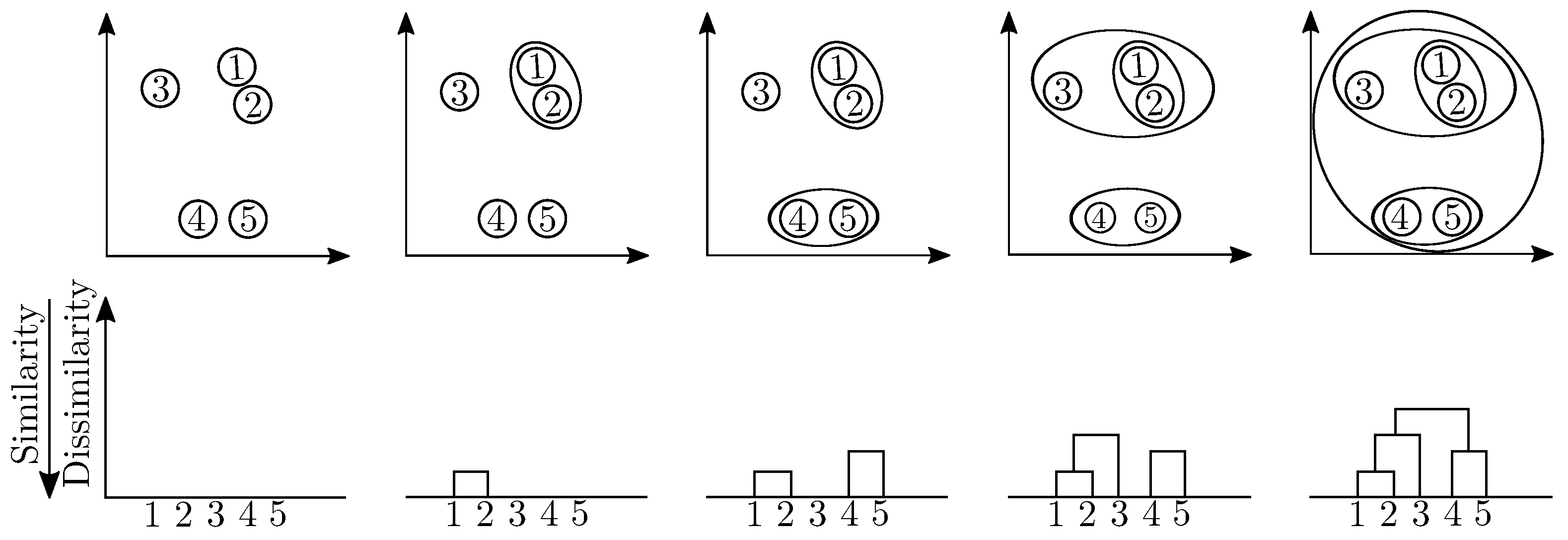
As mentioned above, clustering is the process in which a set of objects or points are grouped into categories or clusters according to a virtual distance measure. Similar points in the same cluster will have a small distance to each other while points in different clusters are dissimilar and thus are at a large distance from one another. Therefore, the dissimilarity between two signals can be used as a virtual distance measure to cluster AE signals. If cross-correlation is used as a measure of similarity of two signals, dissimilarity can be defined as 1 minus the cross-correlation. Normalized cross-correlation is preferred as it can detect the correlation between two signals having a different amplitude. This is of particular interest as the source-sensor distance may vary.

In the developed clustering algorithm, the distance d${}_{xy}$ between two discrete-time signals X${}_n$ and Y${}_n$ (n = 1, …, N) is defined as:

$$d_{xy}=\underset{m}{max}\mid {\widehat{R}}_{xy,\mathrm{norm}}\left(m\right)\mid$$

(1)

where ${\widehat{R}}_{xy,\mathrm{norm}}\left(m\right)$ is equal to the normalized estimation of the cross-correlation of a given lag m, with

$${\widehat{R}}_{xy,\mathrm{norm}}\left(m\right)=\frac{{\widehat{R}}_{xy}\left(m\right)}{\sqrt{{\widehat{R}}_{xx}\left(0\right){\widehat{R}}_{yy}\left(0\right)}}$$

(2)

and

$${\widehat{R}}_{xy}\left(m\right)=\left\{\begin{array}{cc}\sum _{n=0}^{N-m-1}{x}_{n+m}{y}_n,\hfill & m\ge 0\hfill \\ \sum _{n=0}^{N+m-1}{x}_n{y}_{n-m},\hfill & m<0\hfill \end{array}\right.$$

(3)

A correlation coefficient between −1 and 1 can be defined as the maximum of the values of all points. The value 1 means that the two signals show a perfect correlation and are therefore identical, the value 0 means that they are not correlated and therefore not similar at all, and the value −1 means that they are perfectly anti-correlating meaning that they have the same shape, but opposite signs. As the distance cannot be negative and the sign of the signal is not important to distinguish different signals, the absolute value is taken first. The more similar two signals are, the shorter their distance will be. The distance approaches 0 as correlation goes to 1.

The working principle of the algorithm is shown in Figure 1. Each signal forms a separate cluster at the start meaning that the algorithm is agglomerative. These one-signal-clusters are then combined into larger clusters based on their closeness. Two clusters with the shortest distance, i.e., smallest dissimilarity, are merged first. Then, the distance between this newly formed cluster and the other existing clusters needs to be calculated. The calculation of this inter-cluster distance or cophenetic distance can be performed in different ways, among which single (nearest neighbour), complete (furthest neighbour), and average linkage are most commonly used [22]. Single linkage can produce chain-shape clusters meaning that if few data points form a bridge between two clusters, single linkage might unify these two clusters into one. Complete linkage usually gives smaller clusters, but is less sensitive to noise and outliers. Average linkage may also give smaller clusters, but is sensitive to outliers. The approach that is most suitable for the current application was investigated. Complete linkage was used as this gave better results than single and average linkage. In case of average or single linkage, all clusters were connected to each other resulting in one cluster.

Afterwards, the two clusters with the smallest distance are combined and again the cophenetic distance is calculated. These steps are repeated until only one cluster is formed after $N-1$ iterations with N the number of signals. The result can be visualized in a tree structure plot called dendrogram (Figure 1 (bottom)). The dendrogram can be divided in groups based on a user-defined dissimilarity threshold or a required number of clusters.

3. Verification of the Clustering Algorithm on RC Prisms

3.1. Experimental Setup of the RC Prisms

An experimental test program was executed to gather AE data during the corrosion process of RC prisms. The experimental setup with 1D AE monitoring has been presented in Van Steen et al. [5]. Most important specifications are summarized here for completeness.

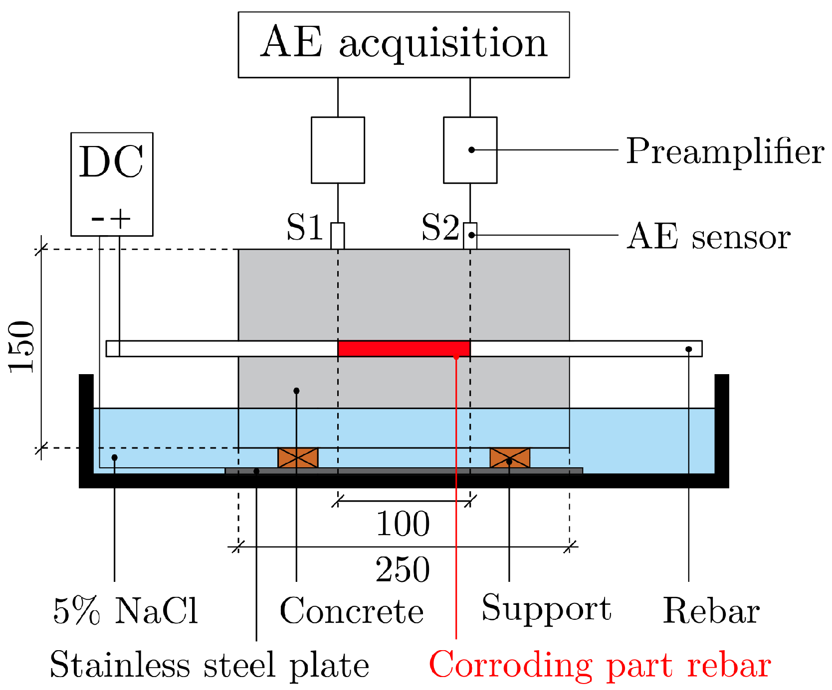
Three corrosion levels (CL) were targeted (1%, 5%, and 10% mass loss) and two rebar types were investigated (ribbed and smooth). Of each type, one sample was made, resulting in six samples. The sample name is based on the corrosion level and rebar type, e.g., CL2-R refers to a sample of the second corrosion level (5% mass loss) having a ribbed rebar. The six RC prisms with dimensions 150 × 150 × 250 mm³ were monitored with a 1D AE sensor setup, using 2 AE sensors per RC sample. The rebars were placed in the center of the sample. A length of 100 mm was bonded to the concrete and was able to corrode. Corrosion was induced with a direct current having a current density of 100 $\mathsf{\mu }$A/cm². The rebar functioned as the anode, whereas a stainless steel plate functioned as the cathode. The samples were partially immersed in a 5% sodium chloride solution. Surface crack measurements were performed once a week with a crack meter having an accuracy of 0.05 mm, using nine measurement points with a spacing of 25 mm. AE monitoring was performed continuously, and only interrupted briefly during the crack measurements.

An AMSY-6 Vallen acquisition system (ASIP-2, advanced version) with six channels was used, allowing monitoring up to three samples at the same time. Broadband piezoelectric sensors with a flat frequency response between 100 and 400 kHz (type AE104A, Fuji Ceramics Corporation) were attached on the specimen surface with hot melt glue (Pattex PTK1). AE sensors with a flat frequency response were preferred as the frequency of interest of the damage sources was unknown and a signal-based analysis was desired. This type of sensor is used as an alternative to the 150 kHz resonance sensor (operating range between 100 and 450 kHz) which is frequently used for damage detection in small-to-medium sized RC samples [12,16,30]. The amplitude threshold, the pre-trigger time, duration discrimination time, and rearm time were set to 40 dB, 20 $\mathsf{\mu }$s, 400 $\mathsf{\mu }$s, and 0.4 ms, respectively. The sampling rate was set to 10 MHz. With 2048 samples being stored, the length of the stored signal was 204.8 $\mathsf{\mu }$s. The digital frequency filter was set between 95 and 850 kHz. This filter was chosen based on the operating frequency range of the sensors which is between 100 and 400 kHz. The accelerated corrosion setup and position of the AE sensors are shown in Figure 2.

As the clustering algorithm is computationally demanding, it will be applied on filtered AE signals. The AE signals are filtered according to a developed filtering protocol as presented in Van Steen and Verstrynge [28]. The threshold-based arrival time is improved by applying the Akaike Information Criterion (AIC). Two criteria were applied to filter the most reliable AE signals. The first criterion is based on the signal-to-noise ratio (SNR), which should be higher than 10. The second criterion evaluates whether the time of arrival (TOA) was accurately picked by AIC, based on the shape of the AIC-value graph. If the slope between the first low point and the global minimum of the AIC graph was higher than −25 $\frac{1}{\mathsf{\mu }\mathrm{s}}$, the estimation with the AIC picker was not found to be accurate. Afterwards, the AE signals were localized in 1D and only the first arriving hit of located events are used for the clustering.

3.2. Results of the RC Prisms

The main objective of the AE clustering is to distinguish between the corrosion process at the anode, and the concrete cracking. In previous work by the authors on small corroded mortar samples, the algorithm allowed distinguishing between corrosion and concrete cracking [29]. Two clusters were obtained and the onset of concrete cracking could be distinguished based on the number of AE events and occurrence in time of the clusters.

In the current research, it was first investigated whether additional sources such as absorption of the sodium chloride solution could be distinguished with the clustering algorithm. Therefore, a set of dummy samples was tested. A first dummy sample (dummy 1) was an uncorroded RC beam subjected to a four-point bending test. Expected damage sources are micro- and macro-cracking of the concrete. A second dummy sample (dummy 2) was an older RC prism that was placed in water to investigate whether signals due to absorption could be detected. The third sample (dummy 3) was a concrete cube with an age of 28 days that was placed in dry conditions (20 °C, 40% RH) after being stored in a humidity chamber (20 °C, 95% RH). Hydration processes as well as a change in ambient humidity level could cause AE signals in this dummy sample. The final dummy sample (dummy 4) was a ribbed rebar that was subjected to accelerated corrosion by placing it in a sodium chloride solution and applying a direct current. In this way, signals related to steel corrosion could be detected. It is assumed that similar processes during the corrosion process itself (such as the formation of salt crystals in the pits, local plastic deformation of the pit, and the expansion of corrosion products [31]) are occurring during corrosion of a rebar without surrounding concrete layer as during corrosion of an RC sample. However, it should be noted that the presence of a concrete layer may influence the AE signal due to a different propagation path. Nonetheless, it was found in previous work by the authors that the AE signals are still alike [5]. A total of 1000 signals (600, 50, 150, and 200 from, respectively, dummies 1, 2, 3, and 4) were randomly selected resulting in a representative share of each damage source based on the occurrence rate of the AE signals during testing of the dummy samples and as expected during the accelerated corrosion tests. On these 1000 signals, which is in terms of order of magnitude in line with the number of AE signals detected during the corrosion tests on the RC prisms, the clustering algorithm was applied.

Figure 3 shows the dendrogram (top) and peak (bottom left) and center (bottom right) frequencies of each AE event versus the ID number of the AE signal. The peak frequency of the signal is defined as the frequency with the maximum signal amplitude in the frequency domain. The center frequency or frequency centroid is defined as the center of gravity of the signal in the frequency domain. The cluster dissimilarity threshold was set in order to obtain two clusters. For the used AE setup, acquisition settings, and AE sensors, it was found in previous work of the authors that the peak and center frequency ranges of signals obtained from micro-cracking, absorption, hydration, and steel corrosion are overlapping (peak frequency between 200 and 260 kHz and center frequency between 170 and 360 kHz) [5]. The signals are characterized by higher frequencies than signals obtained from macro-cracking (peak frequency between 90 and 250 kHz and center frequency between 160 and 290 kHz) [5]. The algorithm is able to distinguish these two groups as visualized in Figure 3. Events belonging to the first cluster (blue) are found in each dummy sample. Events belonging to the second cluster (red) are mainly found in the first dummy sample which is the RC beam subjected to a four-point bending test, being the only one of the dummy samples that should indeed show concrete macro-cracking. Most of these events are characterized by high amplitudes.

The cluster dissimilarity threshold was decreased in order to investigate whether other sources could be distinguished such as corrosion and absorption. The result is shown in Figure 4. When lowering this threshold, four clusters can be obtained. The pink and red cluster can still be assigned to concrete macro-cracking. However, signals belonging to the blue and green cluster still occur in four different dummy samples. Therefore, the clustering algorithm does not allow further differentiating the AE sources. This confirms previous findings that signals originating from corrosion, absorption and concrete micro-cracking are difficult to distinguish from each other [5]. Alternatives to cross-correlation may be investigated such as magnitude-squared coherence [32] or dynamic time warping [33]. However, these alternatives are computationally more demanding. A comparison of the techniques is outside the scope of the current paper. Clustering will further be applied on the accelerated corrosion tests to investigate whether the onset of concrete macro-cracking can be automatically distinguished. It was checked whether similar results were obtained using a different set of signals and this was the case.

Figure 5 shows the clustering result of prism CL3-S which is a sample with a smooth rebar that was corroded until a target corrosion level of 10% mass loss was reached. Crack measurements were performed every week. The grey shaded area on the two bottom figures indicates the time period in which the surface crack must have occurred. This is the period between the last crack measurement where no crack was observed and the first crack measurement where the crack was observed.

Three clusters can be observed. The blue cluster starts from the beginning of the test and contains signals with an average peak frequency of 220 kHz. The number of AE signals of the second cluster (red) increases at the onset of concrete macro-cracking which is confirmed by the grey shaded area. In addition, a decrease in the peak and center frequency can be seen, as observed from the moving average (200 datapoints), which was found to indicate the onset of macro-cracking in previous work [5].

Few AE signals are assigned to the red cluster before the crack was visually observed. As seen in Figure 3, few AE signals due to absorption, hydration and corrosion were seen as similar to the cracking signals and were assigned to the same cluster. Therefore, the early signals assigned to cluster 2 in sample CL3-S may also originate to a limited extent from absorption, hydration or corrosion. Alternatively, it may be the case that cracking started internally and that these signal represent internal cracking, predicting the occurrence of the surface crack that was later observed.

The third cluster (green) represents AE signals due to electromagnetic interference. These signals are typically caused by the presence of fluorescent lamps in the laboratory which cause interference with the AE equipment when switched on or off. They are characterized by one or multiple short peaks in the time domain and by high frequencies (peak frequency higher than 300 kHz) [5]. However, they are not of interest for damage assessment. The clustering algorithm allows filtering these signals.

An overview of the clustering results of all RC prisms is given in Figure 6. The center frequency of each AE signal is shown versus time. The cluster indicating electromagnetic interference is filtered before plotting the results. Using the same cluster dissimilarity threshold for all samples, it can be seen that only one cluster is obtained for the lowest corrosion level as no crack was observed on the surface. This is confirmed with crack width measurements. No significant decrease can be observed for the center frequency as well. For cracked samples, two clusters are obtained. An increase of the number of events belonging to cluster 2 (red) is observed at the onset of macro-cracking. A decrease of the moving average of the center frequency is seen as well which confirms the clustering results.

4. Upscaling to RC Beams

4.1. Experimental Setup of the RC Beams

The clustering algorithm was scaled up towards RC beams. Two test series were performed. For each test series, two beams were considered, further denoted as Beam-1 and Beam-2 for test series 1, and Beam-3 and Beam-4 for test series 2.

The corrosion process was accelerated using the same principle as for the RC prisms. However, it was chosen to place a bottomless tank on top of the beams. The tank was sealed with silicone and the 5% sodium chloride solution was added in this tank. A current density of 50 $\mathsf{\mu }$A/cm² was applied.

For test series 1, the dimensions of the beams were 150 × 200 × 1800 mm³. They were reinforced with a ribbed rebar having a nominal diameter of 14 mm. The concrete cover was 30 mm. Nearly the full length of the rebar (1500 mm) was exposed to corrosion. The same AMSY-6 Vallen acquisition system (ASIP-2, standard version) with six channels and piezoelectric sensors were used as for the RC prisms. The beams were monitored with four AE sensors which were placed in a 2D AE sensor setup. Two sensors were placed at each side of the beam covering the central part of the beam. The distance between the AE sensors along the length of the beam varied for Beam-1 (750 mm) and Beam-2 (500 mm). The amplitude threshold, pre-trigger time, duration discrimination time, and rearm time were set to 40 dB, 200 $\mathsf{\mu }$s, 450 $\mathsf{\mu }$s, and 5 ms, respectively. The sampling rate was set to 5 MHz. With 4096 samples being stored, the total length of the signal was 819.2 $\mathsf{\mu }$s. The digital frequency filter was set between 95 and 850 kHz. Crack measurements were performed once a week with a crack meter having an accuracy of 0.05 mm, using 17 measurement points with a spacing of 100 mm. A schematic representation of the setup and position of the AE sensors is shown in Figure 7.

For the second test series, two RC beams with dimensions 150 × 220 × 3000 mm³ were cast. Two longitudinal rebars with a diameter of 14 mm were used in the tension zone, whereas two longitudinal rebars with a diameter of 12 mm were used in the compression zone. Additionally, stirrups having a diameter of 6 mm were spaced 120 mm at the center and 100 mm beyond. The concrete cover of the longitudinal rebars was 30 mm. Corrosion was induced in a small zone meaning that only 400 mm of the two longitudinal rebars and part of the stirrups could corrode. The position of this zone varied for Beam-3 (symmetrically, at the center) and Beam-4 (asymmetrically, towards the side). To prevent the other parts to corrode, anti-corrosive paint was used to coat the rebars. An AMSY-6 Vallen system (ASIP-2, advanced version) with eight channels was used. The same sensors (flat response 100–400 kHz) were applied. The AE sensor arrangement was kept the same for both beams. Six sensors were used, three on each side of the beam. The distance between the sensors was 1000 mm. The amplitude threshold, pre-trigger time, duration discrimination time, and rearm time were set to 40 dB, 200 $\mathsf{\mu }$s, 500 $\mathsf{\mu }$s, and 5 ms, respectively. The sampling rate was set to 5 MHz. With 4096 samples being stored, the total length of the signal was 819.2 $\mathsf{\mu }$s. As this Vallen system allowed choosing between more digital frequency filters, the digital frequency filter was set between 50 and 500 kHz during acquisition to eliminate electromagnetic noise during the test. However, the lower limit was adapted to 95 kHz during post-processing in order that the results are comparable with the other samples. Crack measurements were performed once a week with a crack meter having an accuracy of 0.05 mm at different locations with a spacing of 50 mm. A schematic representation of the setup and position of the AE sensors is shown in Figure 8.

Also for this sample scale, the clustering algorithm was applied on filtered AE signals. The same post-processing protocol was used as discussed for the RC prisms. Afterwards, the AE signals were localized in 1D. For test series 1, 1D localization was performed along the length of the beam, meaning that sensor pairs 1 and 2, and 3 and 4 were used. For test series 2, the distance between the sensors along the length of the beam was too large for the higher frequency signals to reach the sensors. Therefore, 1D localization was performed along the width of the beam, meaning that sensor pairs 1 and 2, 3 and 4, and 5 and 6 were used. In all cases, clustering was performed based on the signal of the first arriving AE hit of located events.

4.2. Results of the RC Beams

Figure 9 shows the clustering results of Beam-1 (left) and Beam-2 (right). Both peak (top) and center (bottom) frequency of each AE event over time are shown. Moreover, the moving average (200 datapoints) is visualized. The grey shaded area indicates the time period in which the surface crack must have occurred. This is the period between the last crack measurement where no crack was observed and the first crack measurement where the surface crack was visually observed in the zone of interest between the AE sensors. Note that a technical issue with the AE equipment was noticed for Beam-2 during which no AE signals were saved. This time period is indicated by the dashed area.

For Beam-1, the moving average of the peak and center frequency starts to decrease around day 5. At this moment, also an increase of the events belonging to the red cluster can be noticed. Therefore, as this lies within the period that the crack occurred, this indicates the onset of macro-cracking. For Beam-2, an increase of the red cluster was observed as well as a sudden drop of the moving average of the peak frequency around day 6. The average peak and center frequency start to decrease earlier, namely around day 3. To indicate the grey area representing the results of the crack measurements, only the crack measurement points in between the AE sensors are taken into account which is in this case a zone with a length of 500 mm. However, a crack was observed outside the zone covered with AE monitoring on day 6. This crack must have occurred between day 1 (first crack measurement, no crack) and day 6 (second crack measurement, small crack outside AE zone) explaining the group of AE events of the second cluster (red) between days 3 and 5.

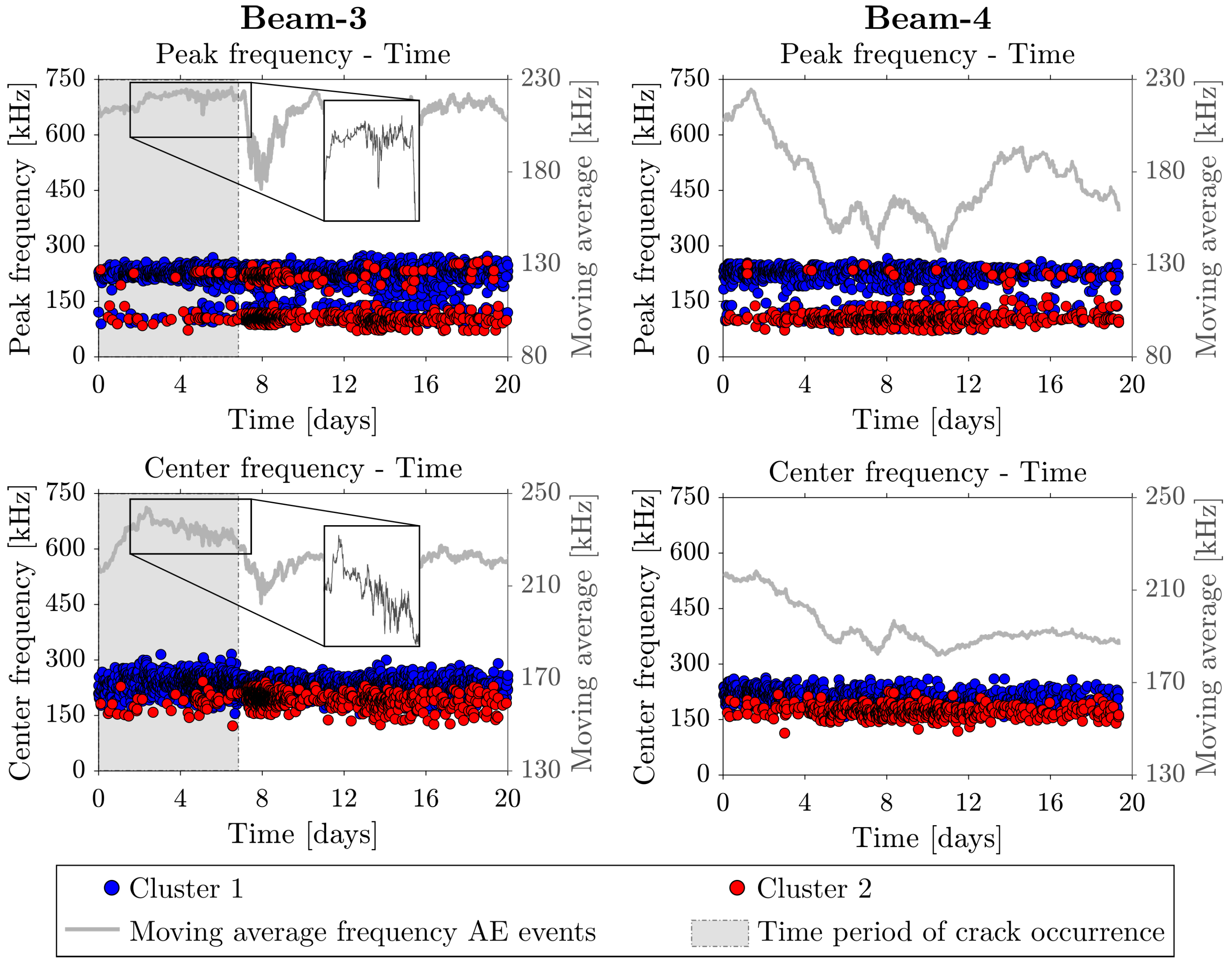
Figure 10 shows the clustering results of Beam-3 (left) and Beam-4 (right). For Beam-3, a small decrease in average peak and center frequency and increase of the number of events of the red cluster is observed around day 4. Indeed, at the first crack measurement, two longitudinal cracks with an average crack width of 0.05 mm were observed. A second and more clear decrease of the peak and center frequencies can be observed around day 8 meaning that the longitudinal cracks grew further. For Beam-4, the moving average of the peak and center frequency starts to decrease from day 2. Unfortunately, no crack measurement was performed at this moment. Based on the observations of the other samples, macro-cracking may have started early during the corrosion test. Besides longitudinal cracks on the top surface, this beam also showed severe cracks at the sides.

It can also be observed from Figure 9 and Figure 10 that the typical accelerated corrosion setup aims at obtaining very high corrosion levels in a short time interval, resulting in early concrete cracking and high damage rates that might not be representative for on-site corrosion damage processes. Therefore, a further validation of the clustering algorithm on samples with slower or natural corrosion rates will be done in future work as a next step towards on-site AE monitoring. Nevertheless, the results of the corroded beams indicate that the developed AE clustering algorithm is able to distinguish the initiation of corrosion-induced concrete macro-cracking.

5. Evaluation of the Clustering Algorithm

In the previous sections, the clustering algorithm was applied on an extensive dataset including dummy samples, RC prisms, and RC beams. AE sensors and AE acquisition settings were kept the same. However, AE setups varied for different sample sizes. On the two sample scales, it can be observed that two clusters can be obtained, which enables to distinguish macro-cracking. In this section, some important parameters and settings are discussed for application of the presented clustering algorithm on datasets obtained during accelerated corrosion in RC.

First, the stability of the clustering algorithm over a range of input settings, or in other words the algorithm’s sensitivity to parameter variations, is discussed. Hierarchical clustering is known to be a clustering method that requires few input settings or parameters [22]. This can be seen as one of the main advantages. Only two input parameters need to be chosen: the type of linkage, and the number of clusters (or value of the dissimilarity threshold). The type of linkage was investigated and complete linkage, which is less susceptible to noise and outliers, was found to be most appropriate for the current application. Average and single linkage resulted in one large cluster with all signals chained to each other. Once an AE signal is assigned to a cluster, the assignment is irreversible. This can be seen as a disadvantage of hierarchical clustering as signals that are incorrectly assigned to an existing cluster in the beginning cannot be moved to a different cluster afterwards. As the algorithm is used on an extensive experimental dataset, it can be observed from the presented results that the algorithm behaves similar in different cases when using complete linkage. Similar results are obtained for different corrosion levels, sample sizes, and AE setups. The number of clusters or the dissimilarity threshold should be chosen as well. In the current analysis, the requirement was found to be twofold after verification on the dummy samples and application on the two sample scales: the maximum number of clusters should be 3 when electromagnetic noise is not filtered beforehand, otherwise it should be 2, in addition, the dissimilarity threshold should be higher than 0.9. It is shown on the dummy samples that dividing the dendrogram in more clusters, no accurate distinction can be made between AE sources. This holds for the current datasets, but should be reconsidered when applying the algorithm on other datasets.

Second, the correctness of the clusters themselves can be discussed, which is less straightforward for hierarchical clustering than for supervised learning algorithms. The results prove that macro-cracking can be distinguished in all presented cases. In this paper, this is validated by crack width measurements. The correctness of the clusters may be influenced by the data quality. It should be mentioned that it is important to filter the AE data first in order to use the most reliable AE signals as it is known that hierarchical clustering algorithms are less robust against noise and outliers [22]. In this paper, we applied the algorithm only on filtered localized AE events. This reduces the probability of the presence of low-frequency noise sources or badly triggered AE signals that influence the results. Still, it is shown that the algorithm is able to identify high-frequency noise signals.

Third, the robustness of the algorithm when different AE sensors and AE acquisition settings are used, should be investigated in future work as this was outside the scope of the current paper. The algorithm works well for the current (extensive) datasets, AE sensors, and AE acquisition settings. It can be concluded that it is accurate for different AE setups. In future work, it should be investigated whether it is applicable for other AE sensors and acquisition settings as well.

6. Conclusions

This paper presented a hierarchical clustering algorithm to differentiate AE sources during the accelerated corrosion process of RC prisms and RC beams. The clustering algorithm is based on the cross-correlation coefficient which is a measure for the similarity between two signals. Dissimilarity (1 minus cross-correlation coefficient) is used as a virtual distance measure to group signals into clusters. The algorithm is applied on two sample scales: RC prisms and RC beams.

On the scale of RC prisms, it was verified that the algorithm is able to distinguish different clusters based on a user-defined dissimilarity threshold. It allows differentiating macro-cracking from micro-cracking and corrosion. In addition, electromagnetic interference can be distinguished, and subsequently filtered. However, analysis of AE signals obtained from several dummy samples revealed that further differentiation between micro-cracking, corrosion, absorption and hydration is not possible as characteristic features of these signals are overlapping. Signals are therefore much alike. Alternatives to cross-correlation can be investigated. Alternatively, supervised learning algorithms may be applied based on the data sets obtained on dummy samples. Still, the algorithm is proven capable of assessing the onset of corrosion-induced cracking. Results were confirmed by crack measurements and a decrease in peak and center frequency, which was previously shown to be a reliable indicator to pinpoint the onset of macro-cracking.

Results were scaled up towards corroding RC beams. Two test series were investigated which vary in position of the corrosion zone and AE sensor layout. In each case, the algorithm is able to distinguish signals originating from macro-cracking and gives an early warning before the crack reaches the surface. The used accelerated corrosion setups aim at obtaining high corrosion levels in a limited time frame which might not be representative for natural corrosion processes on-site. Future work will focus on further validation of the clustering algorithm on samples with slower corrosion rates. Additionally, the effect of sensor type and acquisition settings should be further investigated and verified whether similar findings are observed.

References

- Luo, D.; Li, Y.; Li, J.; Lim, K.S.; Nazal, N.A.M.; Ahmad, H. A Recent Progress of Steel Bar Corrosion Diagnostic Techniques in RC Structures. Sensors 2018, 19, 34. [Google Scholar] [CrossRef] [PubMed] [Green Version]
- Raczkiewicz, W.; Wojcicki, A. Temperature Impact on the Assessment of Reinforcement Corrosion Risk in Concrete by Galvanostatic Pulse Method. Appl. Sci. 2020, 10, 1089. [Google Scholar] [CrossRef] [Green Version]
- Yodsudjai, W.; Pattarakittam, T. Factors influencing half-cell potential measurement and its relationship with corrosion level. Measurement 2017, 104, 159–168. [Google Scholar] [CrossRef]
- Sharma, A.; Sharma, S.; Sharma, S.; Mukherjee, A. Investigation of deterioration in corroding reinforced concrete beams using active and passive techniques. Constr. Build. Mater. 2018, 161, 555–569. [Google Scholar] [CrossRef]
- Van Steen, C.; Nasser, H.; Verstrynge, E.; Wevers, M. Acoustic emission source characterisation of chloride-induced corrosion damage in reinforced concrete. Struct. Health Monit. 2021, 1–21, Advanced online publication. [Google Scholar] [CrossRef]
- Abouhussien, A.A.; Hassan, A.A.A. Evaluation of damage progression in concrete structures due to reinforcing steel corrosion using acoustic emission monitoring. J. Civ. Struct. Health Monit. 2015, 5, 751–765. [Google Scholar] [CrossRef]
- Abouhussien, A.A.; Hassan, A.A.A. Acoustic emission monitoring of corrosion damage propagation in large-scale reinforced concrete beams. J. Perform. Constr. Facil. 2018, 32, 04017133. [Google Scholar] [CrossRef]
- Ing, M.; Austin, S.; Lyons, R. Cover zone properties influencing acoustic emission due to corrosion. Cem. Concr. Res. 2005, 35, 284–295. [Google Scholar] [CrossRef] [Green Version]
- Sharma, A.; Sharma, S.; Sharma, S.; Mukherjee, A. Monitoring invisible corrosion in concrete using a combination of wave propagation techniques. Cem. Concr. Compos. 2018, 90, 89–99. [Google Scholar] [CrossRef]
- Idrissi, H.; Limam, A. Study and characterization by acoustic emission and electrochemical measurements of concrete deterioration caused by reinforcement steel corrosion. NDT E Int. 2003, 36, 563–569. [Google Scholar] [CrossRef]
- Li, W.; Xu, C.; Ho, S.C.M.; Wang, B.; Song, G. Monitoring Concrete Deterioration Due to Reinforcement Corrosion by Integrating Acoustic Emission and FBG Strain Measurements. Sensors 2017, 17, 657. [Google Scholar] [CrossRef] [PubMed] [Green Version]
- Kawasaki, Y.; Wakuda, T.; Kobarai, T.; Ohtsu, M. Corrosion mechanisms in reinforced concrete by acoustic emission. Constr. Build. Mater. 2013, 48, 1240–1247. [Google Scholar] [CrossRef]
- Ohtsu, M.; Tomoda, Y. Corrosion Process in Reinforced Concrete Identified by Acoustic Emission. Mater. Trans. 2007, 48, 1184–1189. [Google Scholar] [CrossRef] [Green Version]
- Leelalerkiet, V.; Shimizu, T.; Tomoda, Y.; Ohtsu, M. Estimation of Corrosion in Reinforced Concrete by Electrochemical Techniques and Acoustic Emission. J. Adv. Concr. Technol. 2005, 3, 137–147. [Google Scholar] [CrossRef] [Green Version]
- Ohtsu, M.; Mori, K.; Kawasaki, Y. Corrosion process and mechanisms of corrosion-induced cracks in reinforced concrete identified by AE analysis. Strain 2011, 47, 179–186. [Google Scholar] [CrossRef]
- Abouhussien, A.A.; Hassan, A.A.A. The Use of Acoustic Emission Intensity Analysis for the Assessment of Cover Crack Growth in Corroded Concrete Structures. J. Nondestruct. Eval. 2016, 35, 52. [Google Scholar] [CrossRef]
- Di Benedetti, M.; Loreto, G.; Matta, F.; Nanni, A. Acoustic emission historic index and frequency spectrum of reinforced concrete under accelerated corrosion. J. Mater. Civ. Eng. 2014, 26, 04014059. [Google Scholar] [CrossRef]
- Zheng, Y.; Zhou, Y.; Zhou, Y.; Pan, T.; Sun, L.; Liu, D. Localized corrosion induced damage monitoring of large-scale RC piles using acoustic emission technique in the marine environment. Constr. Build. Mater. 2020, 243, 118270. [Google Scholar] [CrossRef]
- Morizet, N.; Godin, N.; Tang, J.; Maillet, E.; Fregonese, M.; Normand, B. Classification of acoustic emission signals using wavelets and Random Forests: Application to localized corrosion. Mech. Syst. Signal Process. 2016, 70–71, 1026–1037. [Google Scholar] [CrossRef]
- Piotrkowski, R.; Castro, E.; Gallego, A. Wavelet power, entropy and buspectrum applied to AE signals for damage identification and evaluation of corroded galvanized steel. Mech. Syst. Signal Process. 2009, 23, 432–445. [Google Scholar] [CrossRef]
- Van Dijck, G.; Wevers, M.; Van Hulle, M.M. Wavelet Packet Decomposition for the Identification of Corrosion Type from Acoustic Emission Signals. Int. J. Wavelets Multiresolut. Inf. Process. 2009, 7, 513–534. [Google Scholar] [CrossRef]
- Maimon, O.; Rokach, L. Data Mining and Knowledge Discovery Handbook; Springer: Berlin/Heidelberg, Germany, 2005. [Google Scholar]
- Godin, N.; Huguet, S.; Gaertner, R.; Salmon, L. Clustering of acoustic emission signals collected during tensile tests on unidirectional glass/polyester composite using supervised and unsupervised classifiers. NDT E Int. 2004, 37, 253–264. [Google Scholar] [CrossRef]
- Kravchuk, R.; Landis, E.N. Acoustic emission-based classification of energy dissipation mechanisms during fracture of fiber-reinforced ultra-high performance concrete. Constr. Build. Mater. 2018, 176, 531–538. [Google Scholar] [CrossRef]
- Gutkin, R.; Green, C.J.; Vangrattanachai, S.; Pinho, S.T.; Robinson, P.; Curtis, P.T. On acoustic emission for failure investigation in CFRP: Pattern recognition and peak frequency analyses. Mech. Syst. Signal Process. 2011, 25, 1393–1407. [Google Scholar] [CrossRef]
- Saeedifar, M.; Najafabadi, M.A.; Zarouchas, D.; Toudeshky, H.H.; Jalavand, M. Clustering of interlaminar and intralaminar damages in laminated composites under indentation loading using Acoustic Emission. Compos. Part B 2018, 144, 206–219. [Google Scholar] [CrossRef] [Green Version]
- Calabrese, L.; Campanella, G.; Proverbio, E. Noise removal by cluster analysis after long time AE corrosion monitoring of steel reinforcement in concrete. Constr. Build. Mater. 2012, 34, 362–371. [Google Scholar] [CrossRef]
- Van Steen, C.; Verstrynge, E. Degradation Monitoring in Reinforced Concrete with 3D Localization of Rebar Corrosion and Related Concrete Cracking. Appl. Sci. 2021, 11, 6772. [Google Scholar] [CrossRef]
- Van Steen, C.; Pahlavan, L.; Wevers, M.; Verstrynge, E. Localisation and characterisation of corrosion damage in reinforced concrete by means of acoustic emission and X-ray computed tomography. Constr. Build. Mater. 2019, 197, 21–29. [Google Scholar] [CrossRef]
- Ohno, K.; Ohtsu, M. Crack classification in concrete based on acoustic emission. Constr. Build. Mater. 2010, 24, 2339–2346. [Google Scholar] [CrossRef]
- Winkelmans, M. Fusie van Niet-Destructieve Onderzoekstechnieken Voor Corrosiemonitoring in Chemische Procesinstallaties. Ph.D. Thesis, KU Leuven, Leuven, Belgium, 2004. [Google Scholar]
- Grosse, C.; Reinhardt, H.; Dahm, T. Localization and classification of fracture types in concrete with quantitaive acoustic emission measurement techniques. NDT E Int. 1997, 30, 223–230. [Google Scholar] [CrossRef]
- Chen, S.; Yang, C.; Wang, G.; Liu, W. Similarity assessment of acoustic emission signals and its application in source localization. Ultrasonics 2017, 75, 36–45. [Google Scholar] [CrossRef] [PubMed]
Figure 1.
Working principle of the hierarchical clustering algorithm.
Figure 2.
Schematic representation of the accelerated corrosion setup and 1D AE sensor configuration with two AE sensors (S1–S2).
Figure 3.
Results of the clustering algorithm performed on dummy samples with (top) dendrogram, (bottom left) peak frequency versus ID number of the AE signals, and (bottom right) center frequency versus ID number of the AE signals. The size of the dots depends on the amplitude (in dB) of the AE signal. Expected AE sources are indicated for each group of signal IDs.
Figure 4.
Results of the clustering algorithm performed on dummy samples with (left) dendrogram, and (right) peak frequency versus ID number of the AE signal. The size of the dots depends on the amplitude (in dB) of the AE signal. Expected AE sources are indicated for each group of signal IDs.
Figure 5.
Clustering result of sample CL3-S with (top) dendrogram, (bottom left) peak frequency versus time, and (bottom right) center frequency versus time. The period in which the surface crack occurred is indicated by the grey area.
Figure 6.
Clustering results for all RC prisms represented as center frequency versus time: (top left) CL1-R, (middle left) CL2-R, (bottom left) CL3-R, (top right) CL1-S, (middle right) CL2-S, and (bottom right) CL3-S. The period in which the surface crack occurred is indicated by the grey area.
Figure 7.
Schematic representation of the accelerated corrosion setup and 2D AE sensor configuration (S1–S4) of the first test series of RC beams (Beam-1 and Beam-2).
Figure 8.
Schematic representation of the accelerated corrosion setup and 2D AE sensor configuration (S1–S6) of the second test series of RC beams (Beam-3 and Beam-4).
Figure 9.
Clustering results for Beam-1 (left) and Beam-2 (right) represented as peak frequency (top) and center frequency (bottom) versus time. The period in which the surface crack occurred is indicated by the grey area.
Figure 10.
Clustering results for Beam-3 (left) and Beam-4 (right) represented as peak frequency (top) and center frequency (bottom) versus time. The period in which the surface crack occurred is indicated by the grey area.
Publisher’s Note: MDPI stays neutral with regard to jurisdictional claims in published maps and institutional affiliations. |
© 2022 by the authors. Licensee MDPI, Basel, Switzerland. This article is an open access article distributed under the terms and conditions of the Creative Commons Attribution (CC BY) license (https://creativecommons.org/licenses/by/4.0/).
Share and Cite
MDPI and ACS Style
Van Steen, C.; Verstrynge, E. Signal-Based Acoustic Emission Clustering for Differentiation of Damage Sources in Corroding Reinforced Concrete Beams. Appl. Sci. 2022, 12, 2154. https://0-doi-org.brum.beds.ac.uk/10.3390/app12042154
AMA Style
Van Steen C, Verstrynge E. Signal-Based Acoustic Emission Clustering for Differentiation of Damage Sources in Corroding Reinforced Concrete Beams. Applied Sciences. 2022; 12(4):2154. https://0-doi-org.brum.beds.ac.uk/10.3390/app12042154
Chicago/Turabian StyleVan Steen, Charlotte, and Els Verstrynge. 2022. "Signal-Based Acoustic Emission Clustering for Differentiation of Damage Sources in Corroding Reinforced Concrete Beams" Applied Sciences 12, no. 4: 2154. https://0-doi-org.brum.beds.ac.uk/10.3390/app12042154
Note that from the first issue of 2016, this journal uses article numbers instead of page numbers. See further details here.