A Novel Bayesian Linear Regression Model for the Analysis of Neuroimaging Data

Abstract

In this paper, we propose a novel Machine Learning Model based on Bayesian Linear Regression intended to deal with the low sample-to-variable ratio typically found in neuroimaging studies and focusing on mental disorders. The proposed model combines feature selection capabilities with a formulation in the dual space which, in turn, enables efficient work with neuroimaging data. Thus, we have tested the proposed algorithm with real MRI data from an animal model of schizophrenia. The results show that our proposal efficiently predicts the diagnosis and, at the same time, detects regions which clearly match brain areas well-known to be related to schizophrenia.

1. Introduction

Neuroimaging has undergone a major breakthrough in recent years and has helped in the diagnosis, prognosis, and treatment monitoring of psychiatric disorders. The clinical diagnosis of these disorders is troublesome due to the lack of specific biomarkers [1] and to the fact that many of them share clinical features, thus hindering an accurate diagnosis. Specifically, schizophrenia is one of the most complex pathologies to diagnose [2] since it is commonly confused with other psychotic disorders in up to 20% of cases [3]. As consequence, new tools for the diagnosis of mental disorders are emerging [4,5].

Machine Learning (ML) techniques have emerged as a promising tool for the analysis of neuroimaging data. These algorithms are capable of analyzing any data source, either images (structural or functional), genetic information [6] or behavioral information [7], to carry out an automatic diagnosis of the pathology. Recent approaches based on Support Vector Machine algorithm (SVM) have been applied in Magnetic Resonance Imaging (MRI), showing great results in this field and detecting relevant brain areas involved in the pathology, as well as inferring new useful biomarkers for their diagnosis [8,9,10]. However, although these models have provided accurate results for automatic classification, the lack of interpretability in their results prevents the characterization of the pathology. In particular, in contexts where only a few features are relevant for the problem, it is advisable to detect the informative variables and eliminate the useless ones. For this reason, many authors combine ML models with Feature Selection (FS) approaches, such as the Recursive Feature Elimination (RFE) [11], consisting of the direct elimination of the less representative features, methods based on decision tree formulations, such as Random Forest Importance (RFI) [12,13], or embedded approaches which include L1 or L1–L2 regularizations to promote sparsity, such as Lasso and elastic-net algorithms [14,15]. Nevertheless, in neuroimaging, we have to deal with large datasets, where the number of cases is significantly smaller than the number of variables, and many of these approaches fail in this scenario, tending to over-fit. To avoid this problem, some authors propose Bayesian approaches but work over a reduced set of features [16,17,18], whereas others point to the use of more refined techniques better adapted to the problem needs [19,20,21].

To overcome these limitations, we present a novel formulation for the Bayesian Linear Regression model. Our proposal, called the Dual Bayesian Linear regression model with Feature Selection (DBL-FS), is formulated to work efficiently with a reduced number of samples characterized in high-dimensional spaces, e.g., neuroimaging data. For this purpose, the model is formulated in the dual space and simultaneously includes an Automatic Relevance Determination (ARD) prior over the primal weights to provide the model with FS capabilities so that it can remove irrelevant input features. Here, we have tested our formulation on rodent data in an animal model of schizophrenia that show similar brain anatomical deficits than patients with schizophrenia [22,23,24]. One advantage of using rodent data is a more solid knowledge of the ground truth due to the controlled experimental induction of the pathology.

2. Materials

Rodent MRI data were obtained from the Biomedical Imaging and Instrumentation Group (Biig) of the Gregorio Marañón Hospital. The dataset consisted of 53 rat brain MRI images divided into two groups: healthy rats (N = 24) and pathological rats (N = 29). Pathology was induced by the administration of the viral mimic polyriboinosinic-polyribocytidilic acid (poly I:C) in gestational day 15 to pregnant Wistar rats, since maternal immune stimulation (MIS) is associated with increased risk of onset of schizophrenia in the offspring, with behavioral abnormalities as well as neurophysiological and morphological traits. Model details can be found elsewhere [25,26,27].

All images were preprocessed following the standard preprocessing pipeline in neuroimaging research, using the processing toolbox of the Statistical Parametric mapping software (SPM12) [28], as shown in Figure 1. Output consisted of: White Matter (WM), Gray Matter (GM), and CerebroSpinal Fluid (CSF) regions, with 464,487, 582,467, and 30,702 voxels, respectively.

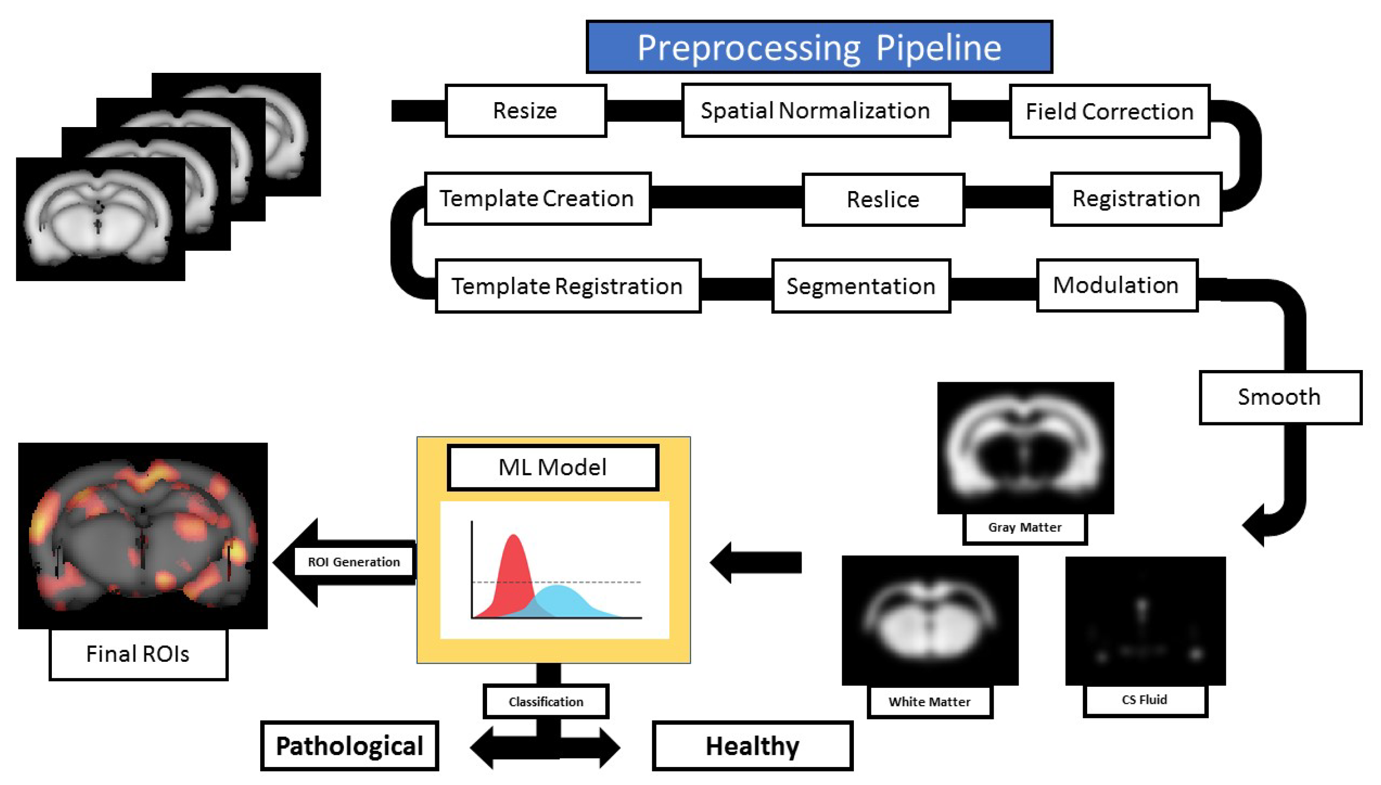
3. Methods

This section introduces the formulation of the proposed Dual Bayesian Linear regression model with Feature Selection (DBL-FS). Later, we also introduce some reference methods that we will use as baselines to show the advantages of the proposed approach together to the experimental setup.

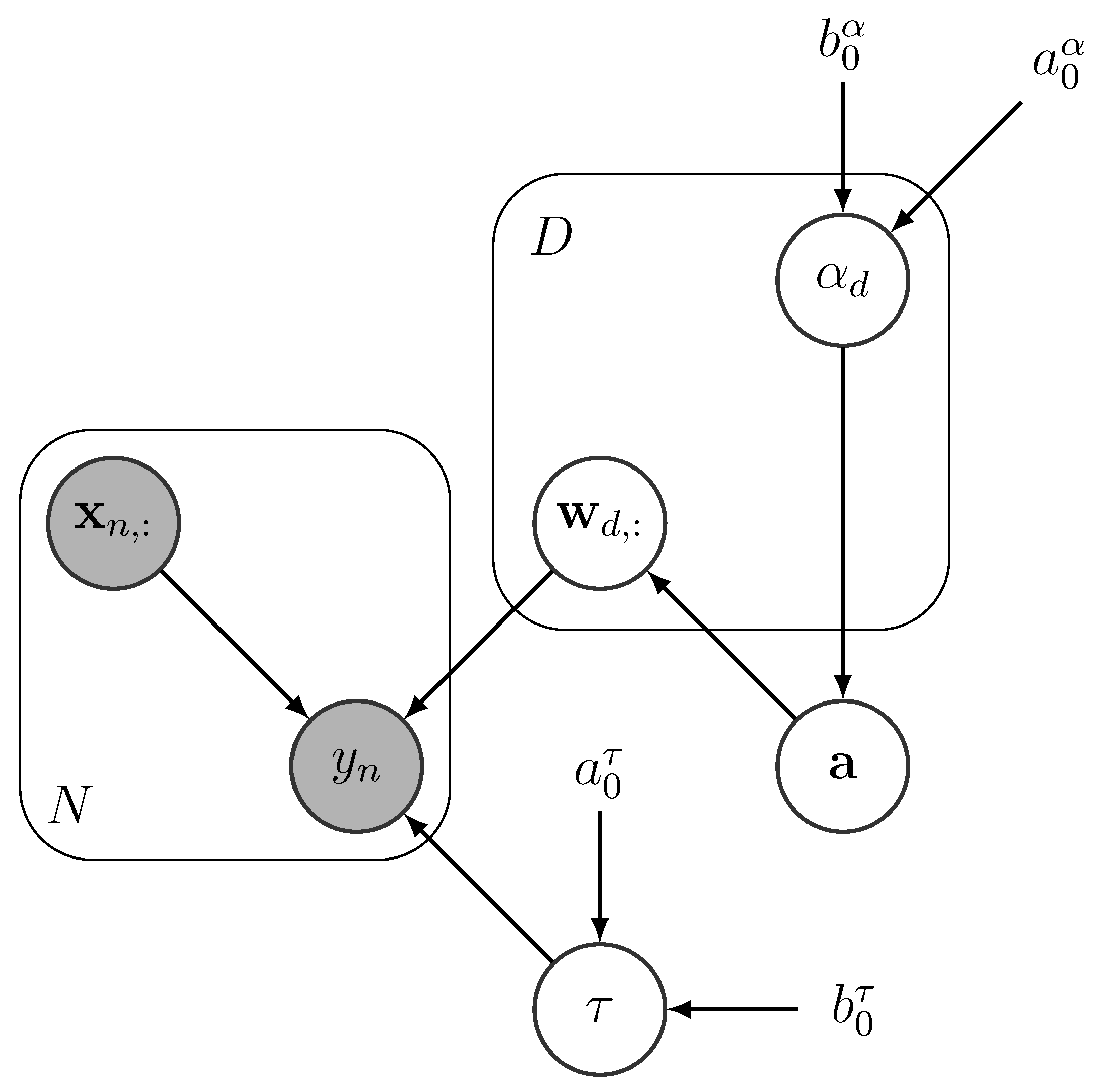
3.1. A Dual Bayesian Linear Regression Model with Feature Selection

3.1.1. Model Definition

The proposed model borrows some ideas from the Bayesian Principal Component Analysis (BPCA) [30] and Bayesian Canonical Correlation Analysis (BCCA) [31] algorithms to endow a Bayesian Linear Regression (BLR) [32] with a dual formulation able to carry out automatic feature selection over the primal variables. This relies on including an ARD prior over the weight matrices to automatically infer the feature relevance in the input feature space by assigning higher/lower relevance values when there are more/less relevant features. Meanwhile, the model works with a formulation in the dual space. In turn, this allows the model to efficiently deal with large data problems by working in the data space while it applies a feature selection over the variable space. In addition, we can exploit the DBL-FS Bayesian formulation to facilitate including prior expert knowledge to guide the FS process. This way, we can guide the learning process and compensate the limited number of samples to train the model.

To define the model, let us consider $\mathbf{X}$ as the observation matrix with the MRI information of N subjects; this way, each row, ${\mathbf{x}}_{n,:}$ for $n=1,\dots ,N$, is a D-dimensional vector containing the brain image of the n-th subject, and each column, ${\mathbf{x}}_{:,d}$ for $d=1,\dots ,D$, contains the information of the d-th voxel over the N subjects. On the other hand, the column vector $\mathbf{y}$ represents the diagnosis labels (control or schizophrenic) for the N subjects under study. Although each label, $y_n$, belongs to the set $\{0,1\}$ (indicating the subject is control or not), for the model formulation, we consider $y_n\in \Re$, and thus, we will generalize the model for regression problems. Later, we will apply a threshold over the model output to classify each subject into one of two categories.

3.1.2. Generative Model

As the graphical model of Figure 2 shows, the generative model of DBL-FS considers that each datum, ${\mathbf{x}}_{n,:}$, is combined with a weight vector $\mathbf{w}$ plus some Gaussian noise to generate the output variable:

$$y_n={\mathbf{x}}_{n,:}\mathbf{w}+\eta ,$$

(1)

where $\eta$ is a Gaussian noise with zero mean and precision $\tau$. In turn, the noise precision is modeled with a gamma distribution with parameters $a_0^{\tau }$, $b_0^{\tau }$:

$$\tau \sim \mathsf{\Gamma }\left(a_0^{\tau },b_0^{\tau }\right)$$

(2)

In addition, DBL-FS considers that the weight associated to the d-th input feature follows a normal distribution:

$$w_d\sim 𝒩\left(0,{\alpha }_d^{-1}\right)d=1,\dots ,D$$

(3)

where its precision, ${\alpha }_d$, is modeled with a gamma distribution as:

$${\alpha }_d\sim \mathsf{\Gamma }\left(a_0^{\alpha },b_0^{\alpha }\right)d=1,\dots ,D$$

(4)

This ARD prior over $w_d$ allows us to obtain the relevance over the elements of $\mathbf{w}$, and therefore, DBL-FS is capable of automatically setting to zero the features that are irrelevant for the problem.

As the model will have to work with MRI data, composed by few samples (less than 100) and tens or hundreds of thousands of voxels, it is clear that working in the primal space is not the most efficient way to proceed. So, we propose to reformulate the model making use of the Representer Theorem [33] (RT). That is, as the RT states that the primal weights of any regression model resulting from minimizing an empirical error (risk) can be expressed as a linear combination of the input data and its equivalent dual coefficients, we can express $\mathbf{w}$ as:

$$\mathbf{w}={\mathbf{X}}^T\mathbf{a}$$

(5)

where $\mathbf{a}$ is a vector of length N containing the dual variables. As we will see later (see Equation (19)), the lower bound that maximizes our variational inference is equivalent to minimizing an empirical cost. This way, the model can be formulated to work in the dual space as:

$$y_n={\mathbf{k}}_{n,:}\mathbf{a}+\eta ,$$

(6)

where ${\mathbf{k}}_{n,:}$ denotes to the n-th row of the linear kernel matrix $\mathbf{K}=\mathbf{X}{\mathbf{X}}^T$. This way, with the dual formulation, the target variables $y_n$, for $n=1,\dots ,N$, are modeled as:

$$y_n\sim 𝒩\left({\mathbf{k}}_{n,:}\mathbf{a},{\tau }^{-1}\right)n=1,\dots ,N.$$

(7)

With this new formulation, the model will be able to work in the space of $\mathbf{a}$, where only N parameters have to be inferred. Thus, model complexity and overfitting risks are drastically reduced, as long as we are able to maintain the feature relevance determination over $\mathbf{w}$, providing the model with feature selection capabilities.

Finally, it is important to note that the model formulation does not need to specifically include the distribution of $\mathbf{a}$ since the relation between $\mathbf{w}$ and $\mathbf{a}$ is deterministic, and therefore, the statistical characterization of $\mathbf{w}$ is also characterizing $\mathbf{a}$.

3.1.3. Variational Inference

Once the generative model is defined, we should evaluate the posterior distribution of the variables to estimate their optimum values. Although, in this case, the posterior distribution is not tractable, we can use variational inference together with the mean-field technique [34] to find an approximation to this posterior $q\left(\mathsf{\Theta }\right)\approx p\left(\mathsf{\Theta }\right|\mathit{y},\mathbf{X})$, where $\mathsf{\Theta }$ contains all model variables. Then, we can define a Lower Bound (LB) using the Kullback–Leibler divergence between the posterior and its approximation; so, maximizing this LB, we can obtain the optimum model parameters. Therefore, using the mean-field approximation to factorize over the posterior, we obtain:

$$p\left(\mathsf{\Theta }\right|\mathit{y},\mathbf{X})\approx q\left(\mathsf{\Theta }\right)=q\left(\mathbf{w}\right)q\left(\mathbf{a}\right)q\left(\alpha \right)q\left(\tau \right),$$

(8)

and we can determine each approximated distribution by calculating:

$$ln\left(q_j^{*}\right)={\mathbb{E}}_{-q_j}[ln\left(p(\mathbf{X},\mathit{y},\mathsf{\Theta })\right)]+const,$$

(9)

where ${\mathbb{E}}_{-q_j}$ implies that we calculate the expectation over all random variables except the j-th variable, and $p(\mathbf{X},\mathit{y},\mathsf{\Theta })$ is the joint probability.

Therefore, we can apply (9) to the joint probability for each random variable to obtain the model update rules. Firstly, the distribution of the dual weights $\mathbf{a}$ is:

$$q\left(\mathbf{a}\right)=\mathcal{N}\left(\mathbf{a}\right|\langle \mathbf{a}\rangle ,{\mathsf{\Sigma }}_a),$$

(10)

with mean and variance determined by:

$$\langle \mathbf{a}\rangle =\langle \tau \rangle {\mathsf{\Sigma }}_a{\mathbf{K}}^{T}y$$

(11)

$${\mathsf{\Sigma }}_a^{-1}=\mathbf{X}\mathrm{diag}\left(\langle \alpha \rangle \right){\mathbf{X}}^T+\langle \tau \rangle {\mathbf{K}}^T\mathbf{K},$$

(12)

where $\mathrm{diag}(\langle \alpha \rangle )$ represents an identity matrix with vector $\alpha$ as the diagonal. The distribution of variable $\alpha$ is:

$$q\left(\alpha \right)=\mathsf{\Gamma }\left(\alpha |a_{\alpha },{\mathbf{b}}_{\alpha }\right),$$

(13)

with parameters

$$a_{\alpha }=a_0^{\alpha }+\frac{D}{2}$$

(14)

$${\mathbf{b}}_{\alpha }=b_0^{\alpha }+\frac{1}{2}\mathrm{diag}\left({\mathbf{X}}^T\langle \mathbf{a}{\mathbf{a}}^T\rangle \mathbf{X}\right),$$

(15)

where ${\alpha }_0^{\alpha }$ and ${\beta }_0^{\alpha }$ are hyperparameters, and the operator diagonal returns a column vector formed by the main diagonal of the matrix. Moreover, the distribution of the noise precision $\tau$ is given by:

$$q\left(\tau \right)=\mathsf{\Gamma }\left(\tau |a_{\tau },b_{\tau }\right),$$

(16)

with parameters

$$a_{\tau }=a_0^{\tau }+\frac{N}{2}$$

(17)

$$b_{\tau }=b_0^{\tau }+\frac{1}{2}(\sum _{n=1}^N{y}_n^2-2Tr\left\{{\mathit{y}}^T\mathbf{K}\langle \mathbf{a}\rangle \right\}+\mathrm{Tr}\left\{{\mathbf{K}}^T\mathbf{K}\langle {\mathbf{aa}}^T\rangle \right\}),$$

(18)

where ${\alpha }_0^{\tau }$ and ${\beta }_0^{\tau }$ are hyperparameters, and $Tr\{\dot{\}}$ is the trace operator. See Appendix A for the full development of these mean field distribution approximations.

Once we have defined the different distributions, the model updates the different random variables in an iterative coordinate-ascent-like optimization where the distribution of each factor is obtained using (10) to (22). This optimization process is guided by the LB cost function defined as:

$$\begin{array}{c}\hfill LB=const+\sum _{n=1}^N\left(\frac{D}{2}+a_0^{\alpha }+1\right)ln\left(b_{\alpha }\right)-\left(\frac{D}{2}+a_0^{\tau }+1\right)ln\left(b_{\tau }\right)-\frac{D}{2}ln\left(\left|{\mathsf{\Sigma }}_a\right|\right),\end{array}$$

(19)

where we analyze its convergence to stop the distribution parameters update. See Appendix B for the full development of the LB.

For an efficient optimization of the model, in practice, we will work in the dual space updating the Equations (10) to (18). However, when the model convergence is reached, we can obtain the approximate posterior distribution of $\mathbf{w}$ as:

$$q\left(\mathbf{w}\right)=\mathcal{N}\left(\mathbf{w}\right|\langle \mathbf{w}\rangle ,{\mathsf{\Sigma }}_w),$$

(20)

with parameters

$$\langle \mathbf{w}\rangle =\langle \mathbf{a}\rangle \mathbf{X}$$

(21)

$${\mathsf{\Sigma }}_w={\mathbf{X}}^T{\mathsf{\Sigma }}_a\mathbf{X}.$$

(22)

Once the model is trained, we can analyze the distribution of $\mathbf{w}$ and check which feature components are zero and, therefore, are eliminated, having an automatic selection of the relevant input voxels. This is due to the fact that, despite working in the dual space, the precision of $\mathbf{w}$ components, $\alpha$, is considered in the distribution of $\mathbf{a}$ (see Equation (12)).

Moreover, the inclusion of a prior over $\alpha$ (see Equation (13)) in the generative model has an additional advantage since we can use it to adapt the prior distribution of $\mathbf{w}$ and include expert knowledge in the model. Thus, in case we want to add more relevance to a particular region (for instance, a neurobiologically meaningful Region of Interest (ROI)), we can initialize the parameters $b_{\alpha }$ associated to the voxels of this region with higher values than the rest to promote that the distribution of $\mathbf{w}$ has also higher values for these voxels. Otherwise, if we do not want to include this expert knowledge, this variable will be uniformly initialized over all voxels.

3.2. Baselines

Here, we present the baseline methods used during the experimental section, whose performances will be compared with those of the proposed DBL-FS model. In particular, we considered three approaches, one baseline aimed to solve regression problems (as DBL-FS) and the other two methods specifically designed to solve classification tasks:

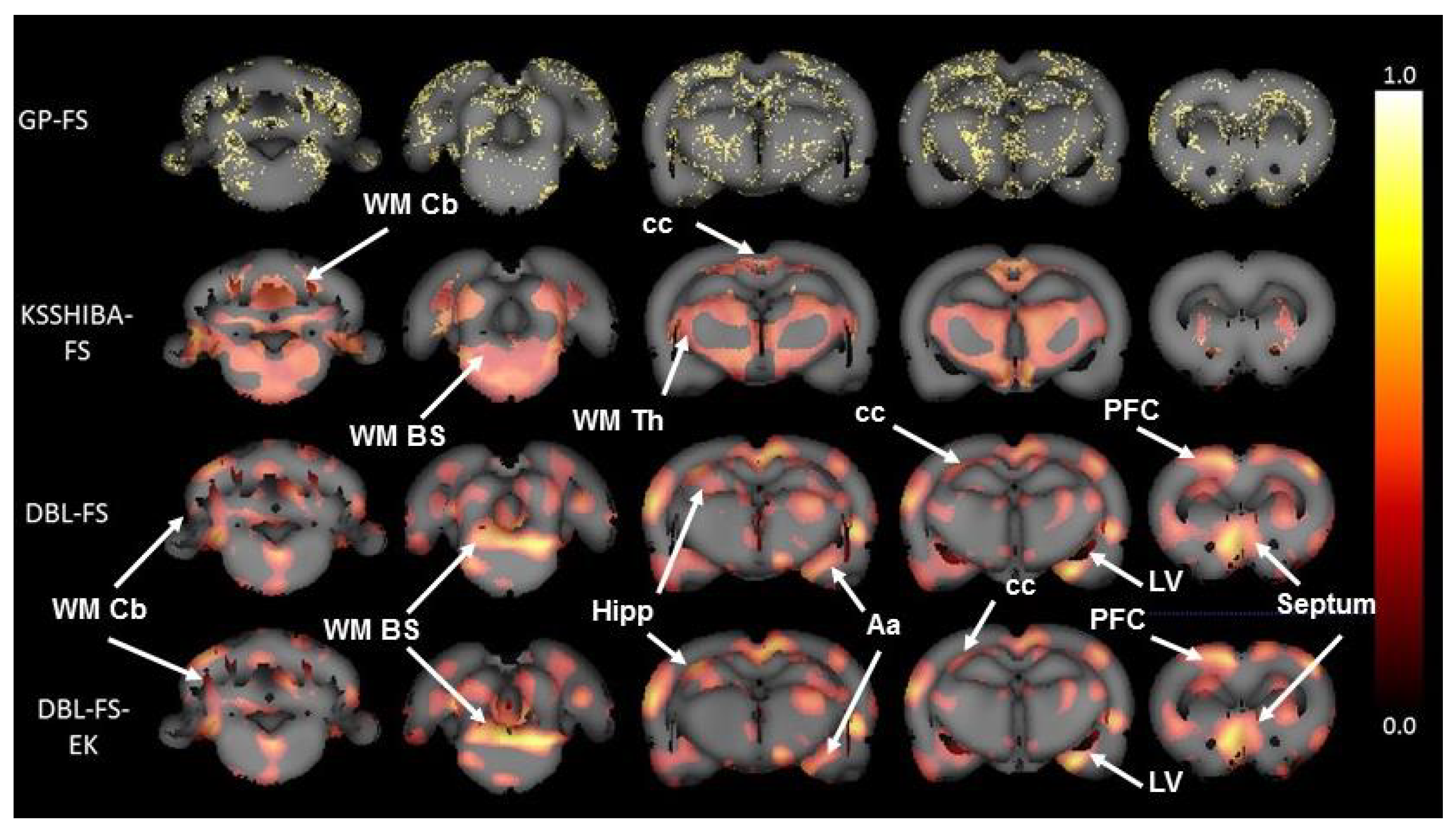
• As the first baseline, we included a regression Gaussian Process (GP) [35], using the implementation provided by the GPy library (available at github accessed on 9 December 2021). We have selected this model since it allows us to define lineal kernels with ARD, so that we can work in the dual space and learn the relevance of the different input features.
• Next, we included an SVM [36] with a linear kernel using the scikit-learn library [37] to also optimize the model in the dual space.
• The last selected baseline is the recently proposed adaptation of Sparse Semi-supervised Heterogeneous Interbattery Bayesian Analysis (SSHIBA) [38] to work in the dual space, the Kernelized SSHIBA (KSSHIBA) [39] is available at github accessed on 29 March 2021. This algorithm can simultaneously combine different data sources or views (in our case, different tissues) in a common latent space providing a low-dimensional representation of the data. In addition, this model can also include an additional output view to categorically model the target variable (patient or control sample), as well as a linear kernel with ARD coefficients over the input features (equivalent to the GP configuration).

Both GP and KSSHIBA use an ARD to determine the relevance of the input features, but they do not have a prior distribution or constraint to force their input weights to be sparse and, therefore, obtain a real FS. Meanwhile, DBL-FS imposes sparsity with the Gamma prior to actually promote zero values in the model weights which, in turn, automatically eliminates the least relevant features.

Furthermore, it is important to mention that deep learning models are not included in this study, as these methods are severely limited by the sample size required to learn the model parameters. Therefore, although models such as convolutional neural networks have promising results in image analysis, they also pose serious challenges when working with datasets of small sample size. Furthermore, we have explored other baselines such as random forests but have not included the results due to their poor results. Nevertheless, all the methods under study will be evaluated with different configurations to be able to analyze different properties and, hence, to carry out an extensive study and analyze their advantages and disadvantages in comparison to our model.

3.3. Experimental Setup

MRI data were standardized to zero mean and unitary standard deviation. As we have a reduced number of subjects (only 53 samples), we have used a Leave-One-Out (LOO) framework to evaluate the model performance. This way, we have trained as many models as available samples, using in each training partition all the subjects except one, which was used afterwards for testing. Then, to evaluate the model performance, we present the results in terms of average accuracy, that is, the percentage of correctly classified test subjects computed over all LOO iterations. Furthermore, since the performance of some methods depends on their initialization we repeated the LOO process 10 times (with different initializations) and depicted the average accuracy over them in order to obtain more statically significant results.

To complete the performance analysis, the result table includes the final number of voxels selected by each model (and their percentage with respect to the total), computed as the average number of voxels used by each model for each LOO iteration and each run.

Regarding the different models under study, we considered several configurations to carry out a more comprehensive analysis and more adequate evaluation of the different methods.

For GPs, we have considered two versions: (1) the standard GP with a linear kernel, denoted as GP, and (2) the previous GP but including ARD capabilities and an FS stage. That is, we first trained a GP with ARD and analyzed the ARD coefficients to select the most relevant features, and then trained a standard GP with the chosen features. Thus, this two-step approach provided a GP with FS capabilities, denoted as GP+FS. For this pruning, we selected the 25% most relevant features in order to compare the performance of this method with DBL-FS. In addition, as both DBL-FS and GPs were formulated for regression problems and our predictive task is a binary classification (0 or 1), we set the threshold to 0.5.

We have implemented two different approaches for SVMs: (1) a standard SVM with linear kernel and (2) an SVM with a Multi-Kernel Learning (MKL) strategy, denoted as MKL-SVM. In the latter case, we independently considered the different tissues (GM, CSF, and WM) and a different linear kernels for each of them, and subsequently, the model learned the combination of these three kernels, including two parameters for their combination. These parameters were defined as scalars multiplying each kernel term, and a subsequent inner LOO was used to find their optimal values. Thus, the defined combinations coefficients gave more or less relevance to each kernel (therefore, to each tissue), providing additional flexibility to the model.

For KSSHIBA, we have included two versions, similarly to what was done in GP: (1) the standard KSSHIBA model and (2) a two-stage version of KSSHIBA (denoted as KSSHIBA+FS), in which KSSHIBA was first trained with ARD functionality, and subsequently, we selected the most relevant features to train the model using this subset of features. For these experiments, we initially had 1000 latent factors, from which the model will automatically prune the irrelevant ones. For FS, we kept the highest 25% of voxels equivalently to the number of selected features from the DBL-FS model.

Finally, we have also defined two approaches for the DBL-FS model, with and without expert knowledge. In the latter one, we have equally initialized the ARD prior for all voxels, setting the parameters a and b of random variable $\alpha$ to 2 and 1, respectively. In the expert knowledge case (denoted as DBL-FS+EK), we have initialized the parameters a and b in such a way that the areas of the prefrontal cortex, ventral hippocampus, and lateral ventricles (which are known to be more intensely affected [23]) had more relevance than the rest. In particular, parameter a was set to 50 and parameter b was fixed to either 1 or $0.001$, depending on whether the voxel belonged to the indicated ROIs or not.

4. Experimental Results

Table 1. Performance of the different methods under study showing the model accuracy and the number of selected voxels (with their percentages with respect to the total). In addition, models with the best accuracy have been highlighted in bold and placed at the bottom of the table, which corresponds to the proposed DBL-FS approaches.

Experiment	Accuracy	# Selected Voxels
GP	67.9%	1,077,656 (100%)
GP+FS	67.9%	269,414 (25%)
SVM	71.6%	1,077,656 (100%)
MKL-SVM	67.9%	1,077,656 (100%)
KSSHIBA	69.8%	1,077,656 (100%)
KSSHIBA+FS	64.1%	269,414 (25%)
DBL-FS	77.3%	287,996 (26.72%)
DBL-FS+EK	77.3%	242,754 (22.52%)

shows the LOO accuracy results for the classification problem together with the number of selected voxels (the approaches without FS used $100\%$). Despite using different initializations in the evaluated models, the results were stable across them with a negligible standard deviation, showing that the initialization hardly influences the results. For this reason, we did not include the standard deviation in Table 1. The results show that GPs, KSSHIBA+FS, and MKL-SVM obtained the worst classification accuracies, while SVM and KSSHIBA achieved the best performances among the baselines. However, DBL-FS and DBL-FS+EK still obtained an improvement of 5.7% in terms of accuracy over the best baseline while learning the most restrictive selection mask. From these results, we need to highlight that (1) KSSHIBA obtained a predictive performance similar to that of SVM while summarizing the information of the original data (distributed in more than ${10}^6$ voxels) in only nine latent variables, and (2) MKL-SVM showed worse results than the standard SVM, probably due to the higher number of hyperparameters it needed to learn in order to perform the MKL, which may be causing overfitting.

Figure 3 shows the brain areas selected by the methods with FS capabilities. As each voxel has an associated weight, the image masks represent the absolute value of these weight magnitudes for the selected of voxels as an indicator of the voxel relevance. In addition, since we have a model for each LOO iteration, Figure 3 displays the average values of these relevances (over all LOO iterations) and includes a normalization of their scales to the range $(0,1)$ to simplify their analysis. As a result, we can observe that the GP-FS selected meaningless voxels in neurobiological terms while KSSHIBA detected well-defined areas corresponding to only WM tissues. Finally, the DBL-FS and DBL-FS+EK approaches obtained well-defined regions in the GM and WM tissues and the CSF, which are interpretable in neurobiological terms. Although both methods provided similar selections, DBL-FS+EK selected a reduced set of voxels.

5. Discussion

This study shows, for the first time, the great advantage of using DBL-FS for the detection and characterization of the morphometric brain changes in a rodent model of schizophrenia. This Bayesian model was adapted for neuroimaging data, characterized by a low sample-to-variable ratio (53 samples vs. 1,077,656 voxels in our case) relying on a dual formulation of the Bayesian Linear Regression model. Furthermore, as the main novelty of this proposal, we combine this dual formulation with a prior over the primal weights to learn the feature relevance over the input features, forcing an automatic FS. Finally, we can exploit the Bayesian nature of the model to include specific prior knowledge to guide the learning process and counterweight the limitations caused by the low sample size of the problem.

Thus, the comparison in terms of performance with the baselines provides clear evidence of the promising results of the proposed DBL-FS model in the characterization of neuroimaging data in mental disorders. Note that DBL-FS is able to largely outperform the baselines in prediction accuracy, showing an advantage of $5.7\%$ in terms of accuracy over the best baseline. In addition, DBL-FS is the only method capable of detecting regions within the three brain tissues that are known to be relevant in the biology of schizophrenia. In this sense, the relevance learned by the GPs is inconsistent between the different LOO iterations, generating a scattered voxel selection and, therefore, a non-localized, unreliable, and uninterpretable mask. On the other hand, KSSHIBA provides a consistent result but only finds relevant regions within WM tissue and, therefore, ignores relevant regions and includes some irrelevant areas.

Analyzing in detail the regions selected by the DBL-FS and DBL-FS+Ek models, we can verify that these areas belong to brain regions whose morphometric changes have been related to schizophrenia, based on the literature. First, as for CSF, the areas with the greatest weight were the most frontal areas of the lateral ventricles and the third ventricle. One of the morphometric hallmarks in schizophrenia is the enlargement of the ventricles [23,40], which is consistent with the learned selection. Second, regarding GM, our model clearly defined anatomical areas, such as the prefrontal cortex (PFC), hippocampus, amygdala, and septum, some of them in both hemispheres. Numerous studies have demonstrated the relevance of the morphological changes of these areas in mental disorders [41,42] together with the disconnection and lack of symmetry between both cerebral hemispheres [43,44]. Similar volumetric abnormalities have also been reported for the animal model used in this study [24,45]. In addition, the method also detected the medial septum, which plays a significant role in dopamine-related disorders such as schizophrenia [46,47] and addictions [48,49,50], which highlights the relevance of this structure in mental disorders. Regarding WM, the method found three well-defined brain areas, the frontal part of corpus callosum and WM tracts of the brainstem and the cerebellum [51,52].

Regarding the inclusion of expert knowledge by means of the $\alpha$ prior, it reveals two interesting behaviors. First, it demonstrates the robustness and potential of the standard DBL-FS since it is able to obtain similar accuracy and roughly similar brain masks to its DBL-FS+EK extension without the need for expert information. Second, the possibility of including expert knowledge makes the model converge faster, and it also refines the brain region selection. It is important to note that, although the expert knowledge guides the inference process, the model is also learning from the data, allowing it to redefine the initial expert knowledge into a specific set of voxels. For instance, looking at Figure 3, we can see that using expert knowledge, we obtain a higher relevance associated with the core of the WM brainstem and hippocampal areas.

6. Conclusions

This article shows a novel Bayesian approach using linear regression to characterize neuroimaging data, tested in an animal model of schizophrenia. The proposed DBL-FS+EK model allowed us to efficiently work with neuroimaging data, characterized by a low sample-to-variable ratio. This is achieved by taking advantage of its Bayesian formulation to work in the dual space while learning a voxel importance for feature selection. Furthermore, the use of a specific prior to force sparsity can be combined with expert knowledge to guide the model. The proposed model was analyzed using MRI data from a rodent model of a schizophrenia database and compared to different baselines. The results provided an outstanding classification performance of DBL-FS+EK, improving the accuracy of the second best classifier, SVM, in ∼6%. Furthermore, looking at the selected voxels and their associated relevance, we can confirm that the proposed model is able to detect biologically relevant areas for the characterization of this disease, as it clearly agrees with known literature.

References

- Carvalho, A.F.; Solmi, M.; Sanches, M.; Machado, M.O.; Stubbs, B.; Ajnakina, O.; Sherman, C.; Sun, Y.R.; Liu, C.S.; Brunoni, A.R.; et al. Evidence-based umbrella review of 162 peripheral biomarkers for major mental disorders. Transl. Psychiatry 2020, 10, 152. [Google Scholar] [CrossRef] [PubMed]
- Widing, L.; Simonsen, C.; Flaaten, C.B.; Haatveit, B.; Vik, R.K.; Wold, K.F.; Åsbø, G.; Ueland, T.; Melle, I. Symptom Profiles in Psychotic Disorder Not Otherwise Specified. Front. Psychiatry 2020, 11, 580444. [Google Scholar] [CrossRef] [PubMed]
- Correll, C.U.; Brevig, T.; Brain, C. Patient characteristics, burden and pharmacotherapy of treatment-resistant schizophrenia: Results from a survey of 204 US psychiatrists. BMC Psychiatry 2019, 19, 362. [Google Scholar] [CrossRef] [PubMed] [Green Version]
- Roberts, L.W.; Chan, S.; Torous, J. New tests, new tools: Mobile and connected technologies in advancing psychiatric diagnosis. NPJ Digit. Med. 2018, 1, 20176. [Google Scholar] [CrossRef] [PubMed]
- Li, Z.; Li, W.; Wei, Y.; Gui, G.; Zhang, R.; Liu, H.; Chen, Y.; Jiang, Y. Deep learning based automatic diagnosis of first-episode psychosis, bipolar disorder and healthy controls. Comput. Med. Imaging Graph. 2021, 89, 101882. [Google Scholar] [CrossRef] [PubMed]
- Trakadis, Y.J.; Sardaar, S.; Chen, A.; Fulginiti, V.; Krishnan, A. Machine learning in schizophrenia genomics, a case-control study using 5090 exomes. Am. J. Med. Genet. Part B Neuropsychiatr. Genet. 2019, 180, 103–112. [Google Scholar] [CrossRef]
- Hettige, N.C.; Nguyen, T.B.; Yuan, C.; Rajakulendran, T.; Baddour, J.; Bhagwat, N.; Bani-Fatemi, A.; Voineskos, A.N.; Chakravarty, M.M.; De Luca, V. Classification of suicide attempters in schizophrenia using sociocultural and clinical features: A machine learning approach. Gen. Hosp. Psychiatry 2017, 47, 20–28. [Google Scholar] [CrossRef]
- Xiao, Y.; Yan, Z.; Zhao, Y.; Tao, B.; Sun, H.; Li, F.; Yao, L.; Zhang, W.; Chandan, S.; Liu, J.; et al. Support vector machine-based classification of first episode drug-naïve schizophrenia patients and healthy controls using structural MRI. Schizophr. Res. 2019, 214, 11–17. [Google Scholar] [CrossRef]
- Guo, Y.; Qiu, J.; Lu, W. Support Vector Machine-Based Schizophrenia Classification Using Morphological Information from Amygdaloid and Hippocampal Subregions. Brain Sci. 2020, 10, 562. [Google Scholar] [CrossRef]
- Jahmunah, V.; Oh, S.L.; Rajinikanth, V.; Ciaccio, E.J.; Cheong, K.H.; Arunkumar, N.; Acharya, U.R. Automated detection of schizophrenia using nonlinear signal processing methods. Artif. Intell. Med. 2019, 100, 101698. [Google Scholar] [CrossRef]
- Brownlee, J. Recursive Feature Elimination (RFE) for Feature Selection in Python. Machine Learning Mastery. 2020. Available online: https://machinelearningmastery.com/rfe-feature-selection-in-python/ (accessed on 25 May 2020).
- Breiman, L. Random forests. Mach. Learn. 2001, 45, 5–32. [Google Scholar] [CrossRef] [Green Version]
- Li, X.; Chen, W.; Zhang, Q.; Wu, L. Building auto-encoder intrusion detection system based on random forest feature selection. Comput. Secur. 2020, 95, 101851. [Google Scholar] [CrossRef]
- Zou, H.; Hastie, T. Regularization and variable selection via the elastic net. J. R. Stat. Soc. Ser. (Stat. Methodol.) 2005, 67, 301–320. [Google Scholar] [CrossRef] [Green Version]
- Amini, F.; Hu, G. A two-layer feature selection method using genetic algorithm and elastic net. Expert Syst. Appl. 2021, 166, 114072. [Google Scholar] [CrossRef]
- Shen, L.; Qi, Y.; Kim, S.; Nho, K.; Wan, J.; Risacher, S.L.; Saykin, A.J. Sparse bayesian learning for identifying imaging biomarkers in AD prediction. In Proceedings of the International Conference on Medical Image Computing and Computer-Assisted Intervention, Beijing, China, 20–24 September 2010; pp. 611–618. [Google Scholar]
- Sabuncu, M.R.; Van Leemput, K. The relevance voxel machine (RVoxM): A self-tuning Bayesian model for informative image-based prediction. IEEE Trans. Med. Imaging 2012, 31, 2290–2306. [Google Scholar] [CrossRef] [Green Version]
- Sabuncu, M.R. A sparse Bayesian learning algorithm for longitudinal image data. In Proceedings of the International Conference on Medical Image Computing and Computer-Assisted Intervention, Munich, Germany, 5–9 October 2015; pp. 411–418. [Google Scholar]
- Parrado-Hernández, E.; Gómez-Verdejo, V.; Martínez-Ramón, M.; Shawe-Taylor, J.; Alonso, P.; Pujol, J.; Menchón, J.M.; Cardoner, N.; Soriano-Mas, C. Discovering brain regions relevant to obsessive–compulsive disorder identification through bagging and transduction. Med. Image Anal. 2014, 18, 435–448. [Google Scholar] [CrossRef]
- Gómez-Verdejo, V.; Parrado-Hernández, E.; Tohka, J. Sign-consistency based variable importance for machine learning in brain imaging. Neuroinformatics 2019, 17, 593–609. [Google Scholar] [CrossRef] [Green Version]
- Sevilla-Salcedo, C.; Gómez-Verdejo, V.; Tohka, J. Regularized Bagged Canonical Component Analysis for Multiclass Learning in Brain Imaging. Neuroinformatics 2020, 18, 641–659. [Google Scholar] [CrossRef]
- Grimm, O.; Gass, N.; Weber-Fahr, W.; Sartorius, A.; Schenker, E.; Spedding, M.; Risterucci, C.; Schweiger, J.I.; Böhringer, A.; Zang, Z.; et al. Acute ketamine challenge increases resting state prefrontal-hippocampal connectivity in both humans and rats. Psychopharmacology 2015, 232, 4231–4241. [Google Scholar] [CrossRef]
- Hadar, R.; Soto-Montenegro, M.L.; Götz, T.; Wieske, F.; Sohr, R.; Desco, M.; Hamani, C.; Weiner, I.; Pascau, J.; Winter, C. Using a maternal immune stimulation model of schizophrenia to study behavioral and neurobiological alterations over the developmental course. Schizophr. Res. 2015, 166, 238–247. [Google Scholar] [CrossRef] [Green Version]
- Romero-Miguel, D.; Casquero-Veiga, M.; MacDowell, K.S.; Torres-Sanchez, S.; Garcia-Partida, J.A.; Lamanna-Rama, N.; Romero-Miranda, A.; Berrocoso, E.; Leza, J.C.; Desco, M.; et al. A Characterization of the Effects of Minocycline Treatment During Adolescence on Structural, Metabolic, and Oxidative Stress Parameters in a Maternal Immune Stimulation Model of Neurodevelopmental Brain Disorders. Int. J. Neuropsychopharmacol. 2021, 24, 734–748. [Google Scholar] [CrossRef] [PubMed]
- Ozawa, K.; Hashimoto, K.; Kishimoto, T.; Shimizu, E.; Ishikura, H.; Iyo, M. Immune activation during pregnancy in mice leads to dopaminergic hyperfunction and cognitive impairment in the offspring: A neurodevelopmental animal model of schizophrenia. Biol. Psychiatry 2006, 59, 546–554. [Google Scholar] [CrossRef] [PubMed]
- Zhu, F.; Zheng, Y.; Liu, Y.; Zhang, X.; Zhao, J. Minocycline alleviates behavioral deficits and inhibits microglial activation in the offspring of pregnant mice after administration of polyriboinosinic–polyribocytidilic acid. Psychiatry Res. 2014, 219, 680–686. [Google Scholar] [CrossRef] [PubMed]
- Meyer, U.; Feldon, J. To poly (I: C) or not to poly (I: C): Advancing preclinical schizophrenia research through the use of prenatal immune activation models. Neuropharmacology 2012, 62, 1308–1321. [Google Scholar] [CrossRef]
- Casquero-Veiga, M.; Garcia-Garcia, D.; MacDowell, K.S.; Perez-Caballero, L.; Torres-Sanchez, S.; Fraguas, D.; Berrocoso, E.; Leza, J.C.; Arango, C.; Desco, M.; et al. Risperidone administered during adolescence induced metabolic, anatomical and inflammatory/oxidative changes in adult brain: A pet and mri study in the maternal immune stimulation animal model. Eur. Neuropsychopharmacol. 2019, 29, 880–896. [Google Scholar] [CrossRef]
- Valdes Hernandez, P.A.; Sumiyoshi, A.; Nonaka, H.; Haga, R.; Aubert Vasquez, E.; Ogawa, T.; Iturria Medina, Y.; Riera, J.J.; Kawashima, R. An in vivo MRI template set for morphometry, tissue segmentation, and fMRI localization in rats. Front. Neuroinform. 2011, 5, 26. [Google Scholar]
- Bishop, C.M. Bayesian PCA. In Advances in Neural Information Processing Systems; The MIT Press: Cambridge, MA, USA, 1999; pp. 382–388. [Google Scholar]
- Klami, A.; Virtanen, S.; Kaski, S. Bayesian canonical correlation analysis. J. Mach. Learn. Res. 2013, 14, 965–1003. [Google Scholar]
- Bishop, C.M. Pattern recognition. Mach. Learn. 2006, 128, 1–39. [Google Scholar]
- Schölkopf, B.; Herbrich, R.; Smola, A.J. A generalized representer theorem. In Proceedings of the International Conference on Computational Learning Theory, Amsterdam, The Netherlands, 16–19 July 2001; pp. 416–426. [Google Scholar]
- Blei, D.M.; Kucukelbir, A.; McAuliffe, J.D. Variational Inference: A Review for Statisticians. J. Am. Stat. Assoc. 2017, 112, 859–877. [Google Scholar] [CrossRef] [Green Version]
- Rasmussen, C.E. Gaussian processes in machine learning. In Summer School on Machine Learning; Springer: Berlin/Heidelberg, Germany, 2003; pp. 63–71. [Google Scholar]
- Steinwart, I.; Christmann, A. Support Vector Machines; Springer Science & Business Media: New York, NY, USA, 2008. [Google Scholar]
- Pedregosa, F.; Varoquaux, G.; Gramfort, A.; Michel, V.; Thirion, B.; Grisel, O.; Blondel, M.; Prettenhofer, P.; Weiss, R.; Dubourg, V.; et al. Scikit-learn: Machine Learning in Python. J. Mach. Learn. Res. 2011, 12, 2825–2830. [Google Scholar]
- Sevilla-Salcedo, C.; Gómez-Verdejo, V.; Olmos, P.M. Sparse semi-supervised heterogeneous interbattery bayesian analysis. Pattern Recognit. 2021, 120, 108141. [Google Scholar] [CrossRef]
- Sevilla-Salcedo, C.; Guerrero-López, A.; Olmos, P.M.; Gómez-Verdejo, V. Bayesian Sparse Factor Analysis with Kernelized Observations. arXiv 2020, arXiv:2006.00968. [Google Scholar]
- Styner, M.; Lieberman, J.A.; McClure, R.K.; Weinberger, D.R.; Jones, D.W.; Gerig, G. Morphometric analysis of lateral ventricles in schizophrenia and healthy controls regarding genetic and disease-specific factors. Proc. Natl. Acad. Sci. USA 2005, 102, 4872–4877. [Google Scholar] [CrossRef] [PubMed] [Green Version]
- Rapado-Castro, M.; Villar-Arenzana, M.; Janssen, J.; Fraguas, D.; Bombin, I.; Castro-Fornieles, J.; Mayoral, M.; González-Pinto, A.; de la Serna, E.; Parellada, M.; et al. Fronto-Parietal Gray Matter Volume Loss Is Associated with Decreased Working Memory Performance in Adolescents with a First Episode of Psychosis. J. Clin. Med. 2021, 10, 3929. [Google Scholar] [CrossRef]
- Wen, D.; Wang, J.; Yao, G.; Liu, S.; Li, X.; Li, J.; Li, H.; Xu, Y. Abnormality of subcortical volume and resting functional connectivity in adolescents with early-onset and prodromal schizophrenia. J. Psychiatr. Res. 2021, 140, 282–288. [Google Scholar] [CrossRef]
- Guo, S.; Kendrick, K.M.; Zhang, J.; Broome, M.; Yu, R.; Liu, Z.; Feng, J. Brain-wide functional inter-hemispheric disconnection is a potential biomarker for schizophrenia and distinguishes it from depression. Neuroimage Clin. 2013, 2, 818–826. [Google Scholar] [CrossRef] [Green Version]
- Boklage, C.E. Schizophrenia, brain asymmetry development, and twinning: Cellular relationship with etiological and possibly prognostic implications. Biol. Psychiatry 1977, 12, 19–35. [Google Scholar]
- Casquero-Veiga, M.; Romero-Miguel, D.; MacDowell, K.S.; Torres-Sanchez, S.; Garcia-Partida, J.A.; Lamanna-Rama, N.; Gómez-Rangel, V.; Romero-Miranda, A.; Berrocoso, E.; Leza, J.C.; et al. Omega-3 fatty acids during adolescence prevent schizophrenia-related behavioural deficits: Neurophysiological evidences from the prenatal viral infection with PolyI: C. Eur. Neuropsychopharmacol. 2021, 46, 14–27. [Google Scholar] [CrossRef]
- Bortz, D.M.; Grace, A.A. Medial septum activation produces opposite effects on dopamine neuron activity in the ventral tegmental area and substantia nigra in MAM vs. normal rats. NPJ Schizophr. 2018, 4, 17. [Google Scholar] [CrossRef] [Green Version]
- Takeuchi, Y.; Nagy, A.; Barcsai, L.; Li, Q.; Ohsawa, M.; Mizuseki, K.; Berényi, A. The medial septum as a potential target for treating brain disorders associated with oscillopathies. Front. Neural Circuits 2021, 15, 701080. [Google Scholar] [CrossRef] [PubMed]
- McGlinchey, E.M.; Aston-Jones, G. Dorsal hippocampus drives context-induced cocaine seeking via inputs to lateral septum. Neuropsychopharmacology 2018, 43, 987–1000. [Google Scholar] [CrossRef] [PubMed] [Green Version]
- Pantazis, C.B.; Aston-Jones, G. Lateral septum inhibition reduces motivation for cocaine: Reversal by diazepam. Addict. Biol. 2020, 25, e12742. [Google Scholar] [CrossRef] [PubMed]
- Gárate-Pérez, M.F.; Méndez, A.; Bahamondes, C.; Sanhueza, C.; Guzmán, F.; Reyes-Parada, M.; Sotomayor-Zárate, R.; Renard, G.M. Vasopressin in the lateral septum decreases conditioned place preference to amphetamine and nucleus accumbens dopamine release. Addict. Biol. 2021, 26, e12851. [Google Scholar] [CrossRef] [PubMed]
- Yang, M.; Gao, S.; Zhang, X. Cognitive deficits and white matter abnormalities in never-treated first-episode schizophrenia. Transl. Psychiatry 2020, 10, 368. [Google Scholar] [CrossRef]
- Kim, S.E.; Jung, S.; Sung, G.; Bang, M.; Lee, S.H. Impaired cerebro-cerebellar white matter connectivity and its associations with cognitive function in patients with schizophrenia. NPJ Schizophr. 2021, 7, 38. [Google Scholar] [CrossRef]