A Deep Learning Ensemble Method to Visual Acuity Measurement Using Fundus Images

Abstract

Visual acuity (VA) is a measure of the ability to distinguish shapes and details of objects at a given distance and is a measure of the spatial resolution of the visual system. Vision is one of the basic health indicators closely related to a person’s quality of life. It is one of the first basic tests done when an eye disease develops. VA is usually measured by using a Snellen chart or E-chart from a specific distance. However, in some cases, such as the unconsciousness of patients or diseases, i.e., dementia, it can be impossible to measure the VA using such traditional chart-based methodologies. This paper provides a machine learning-based VA measurement methodology that determines VA only based on fundus images. In particular, the levels of VA, conventionally divided into 11 levels, are grouped into four classes and three machine learning algorithms, one SVM model and two CNN models, are combined into an ensemble method in order to predict the corresponding VA level from a fundus image. Based on a performance evaluation conducted using randomly selected 4000 fundus images, we confirm that our ensemble method can estimate with 82.4% of the average accuracy for four classes of VA levels, in which each class of Class 1 to Class 4 identifies the level of VA with 88.5%, 58.8%, 88%, and 94.3%, respectively. To the best of our knowledge, this is the first paper on VA measurements based on fundus images using deep machine learning.

1. Introduction

According to World Health Organization (WHO) statistics, the number of people with visual morbidity worldwide, as of 2020, is in excess of 299.1 million, of which 49.1 million is blind [1]. Visual sight is closely related to the quality of daily human life, such as safe walking, driving, and working; thus, regular eye health screening is essential to maintain eye health. Visual Acuity (VA) is a measure of the ability of the eye to distinguish shapes and the details of objects at a given distance. It is one of the essential indications of health. It is the most commonly used intuitive measure of the visual system’s performance. The measurement of VA provides a baseline recording of VA, aids examination and diagnosis of eye disease or refractive errors, assesses any vision changes, and measures the outcomes of cataract or other surgery.

VA may be measured in various ways, depending on various conditions, such as illuminance. However, the measurement of VA needs to be consistent in order to detect any changes in vision. The general ways of VA measurement are (1) multi-letter Snuellen or E chart (2) plain occluder, card or tissue, (3) pinhole occluder, (4) touch or flashlight, or (5) patient’s documentation. The general procedure for VA measurement recommended by the US national library of medicine can be as follows [2]:

• Position the patient, sitting or standing, at a distance of 6 m from the chart;
• Test the eyes one at a time, at first without any spectacles (if worn);
• Ask the patient to cover one eye with a plain occluder, card or tissue;
• Ask the patient to read from the top of the chart and from left to right;
• Record the VA for each eye in the patient‘s notes, stating whether it is with or without correction (spectacles). For example, Right VA = 0.1 with correction, Left VA = 0.2 with correction.
• …

In this procedure, the communication between VA examiner and examinee is essential to measure VA. However, it is not suitable or impossible to use the classical ways of measuring VA in the following occasions:

• When the patient is unable to use the measurement tool due to mobility difficulties;
• When the patient is unconscious state or lack of cooperation during the evaluation;
• When malingering should be strongly suspected;
• When an infant or a very young patient requires the measurement of VA.

In particular, continuous visual acuity measurement is necessary to secure the quality of life after regaining consciousness for patients who remain unconscious for a long time. However, since the existing method of measuring vision requires the patient to have a conversation with a tester, it is impossible to measure the vision of a prolonged unconscious. In addition, in a situation, such as the recent COVID-19 pandemic, as social isolation is prolonged, patients feel that it is harder to visit hospitals than before. For this reason, it becomes challenging to manage people’s visual sight via the traditional method of measuring eyesight.

This paper provides a vision measurement method using deep learning-based ensemble methodology using fundus images. In this paper, we would overcome the following two problems:

• How can we measure the VA from an examinee who cannot communicate with the VA examiner or tries to present an incorrect VA value?
• How can we achieve a more accurate classifier when a dataset is fairly biased to certain classes in terms of the number of sample data?

Fundus photography involves photographing the rear of an eye, which is also known as the fundus. It is a photo image most popularly used in examining more than 38 types of eye diseases, such as age-related macular degeneration, neoplasm of choroid, chorior-retinal inflammation or scars, glaucoma, retinal detachment and defects, and so on. Fundus imaging has been advanced to decrease preventable visual morbidity by allowing easy and timely fundus screening. In particular, the usability and portability of fundus screening have been continuously advanced for the last two decades. Furthermore, recently, there have been significant technological advances that have radicalized retinal photography. Improvements in telecommunications and smartphones are two remarkable breakthroughs that have made ophthalmic screening in remote areas a realizable possibility [3].

We address the above first problem with the high availability of fundus images. We would estimate the VA by capturing a fundus image from a VA examinee and using a VA classifier based on a deep machine learning technique. In this paper, 11 levels from 0.0 to 1.0 (step by 0.1) of VA levels are grouped into four classes according to ophthalmologist doctor’s needs.

To tackle the second problem, we adopt an ensemble approach consisting of three machine learning models. In the medical field, it is very difficult to obtain a balanced size of a medical dataset because the dataset of normal cases is much larger than those of abnormal cases. The dataset of VA measurement results has the same issue; the cases of a lower VA level, in reality, are much less than those of a higher VA level. For this reason, it is difficult to adopt a classical CNN model for such unbalanced datasets of VA levels in a classical way. In our ensemble approach, three machine learning models and techniques are combined to the classification of VA level groups or VA levels using their best classification performance.

The contributions of this paper are to

• to present a deep-learning-based VA measurement approach using fundus images;
• to demonstrate the feasibility and effectiveness of an ensemble approach to overcome the difficulties of obtaining datasets with a balanced size, and
• to present a VA measurement alternative for the examinee who is not easy or has no possible way to communicate with the VA examiner.

To the best of our knowledge, this is the first paper on the VA measurement based on fundus images using machine learning.

This paper is organized as follows: In Section 2, we present related work relevant to this work. In Section 3, we present a simple description on fundus images and the datasets consisting of fundus image and VA measurement data that we obtain from hospitals. Section 4 presents the main idea of our approach, a deep learning-based ensemble methodology for VA Measurement. We discuss the reason why an ensemble method is appropriate for our work and individual machine learning techniques comprising the ensemble method. In Section 5, we present the validation results of our proposed 4-Class VA classifier based on fundus images with various metrics of machine learning performance evaluation and a comparison of our ensemble method against the VGG-19-based CNN model. Finally, we conclude this paper in Section 6.

2. Related Work

Colenbrander [4] discusses the classical methods for VA measurement. Recently, some approaches to VA measurement have presented using various tools and smartphones [5,6,7]. Recently, ML using DNN has been actively used to diagnose, predict, and suggest medical treatment methods [8,9,10,11,12]. ML using DNN is also being actively used in ophthalmology [13,14,15,16,17,18]. Closely related to this study, there are some VA measurements using DNN [18,19,20,21]. For instance, Alexeeff et al. [21] develop a prediction model of final corrected distance visual acuity (CDVA) after cataract surgery, using machine learning algorithms based on electronic health record data. The fundus image is a universal and most actively used ophthalmic image for the diagnosis of various ophthalmic diseases. For this reason, recently, ML-based AI using this fundus image as training data are being actively studied for classification and prediction of eye diseases, such as diabetic retinopathy, glaucoma, and age-related macular degeneration [22,23,24,25,26,27]. However, to our best knowledge, no previous work presents ML for VA measurement, using fundus images and VA measurements of personals.

3. Datasets: Fundus Images and Vision Measurements

In this study, a vision acuity classification model is implemented based on personal’s vision data and the relevant fundus images.

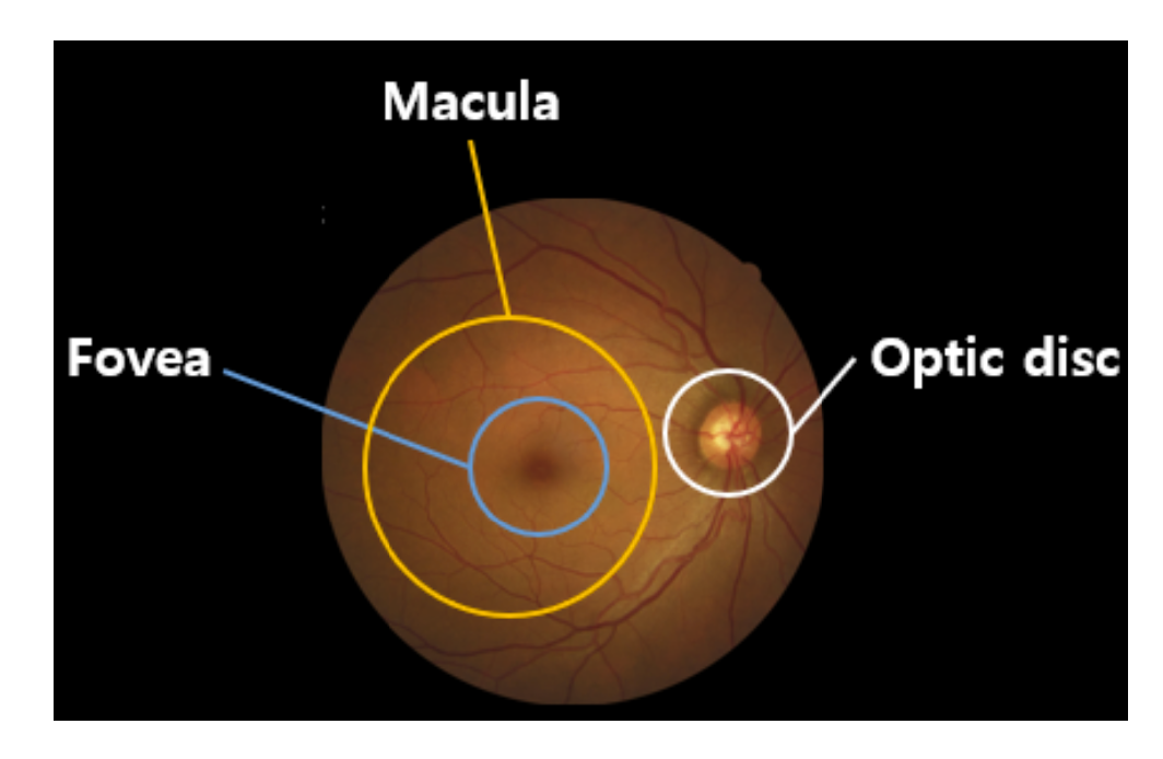
Fundus photography involves taking pictures of the back of the eye, also known as fundus. A special fundus camera consisting of a complex microscope attached to a flash-enabled camera is used for fundus photography. The main structures that can be visualized in fundus photography are the macula, the optic disc, and mid-peripheral retina with retinal vessels.

In Figure 1, the retina is the innermost layer of light-sensitive tissue in most vertebrates and some mollusks. The optics of the eye make the visual world concentrated on the retina into a two-dimensional image, and the retina converts the image into an electrical nerve stimulus to the brain to create a visual perception. The retina functions similarly to the camera’s film or image sensor. The optic disc is the point where the axons of retinal ganglion cells converge and leave the eye. The optic disc in the normal human eye carries 1–1.2 million afferent nerve fibers from the eye to the brain.The optic disc is also the entry point for the major blood vessels that supply blood to the retina. The oval yellow area surrounds the fovea near the center of the retina of the eye, the area of sharpest vision. The human macula is about 5.5 mm (0.22 inches) in diameter. The macula of the human eye is where light is focused by the structures in front of the eye (cornea and lens). The photoreceptor cells in the macula are connected to nerve fibers and transmit visual information to the brain.

3.1. Datasets: Fundus Images and Patient’s Vision Data

The vision chart data and fundus images of patients are obtained from 79,798 patients from February 2016 to January 2021 at the Department of Ophthalmology at Gyeongsang National University Changwon Hospital. The procedures used in this study followed the principles of the Declaration of Helsinki. The requirement for obtaining informed patient consent was waived by the institutional review board of Gyeongsang National University, Changwon Hospital (GNUCH 2021-05-007) due to the retrospective nature of the study.

The fundus images we used in this study are acquired in BMP files by an automation program in AutoIt. A fundus image is selected after matching the personal ID of a fundus image to a personal integrated vision information record. The original data used in this study are anonymized before its use. In this study, retrieving personal vision information necessary for machine learning is conducted in two stages: coupling fundus images and personal vision information and pre-processing of fundus images. In the first stage, we extract the vision acuity information from the medical charts of 79,798 patients with the keywords ‘VA (Vision Acuity)’, ‘BCVA (Best Corrected VA)’, and ‘CVA (Corrected VA)’ and reshape, for our purpose, personal vision datasets of 60,021 visual acuity information, of which each has a corresponding fundus image.

Initially, we have a total of 102,237 fundus images coupled with individual personal VA measurements. We use the personal id and the date of a funds image taken when coupling a fundus image and personal vision data. Ultimately, we obtained 79,800 images by this matching. Furthermore, 55,152 fundus images of them are used as data sets for machine learning.

We abstract the classical 11 levels of VA measurements (0.0–1.0, step by 0.1) into four groups as shown in

Table 1. Our VA classification.

Conventional VA Class	New VA Classes	Features
0.0–0.05	Class 1	Macular pigmentation and depigmentation findings Macular bleeding and ischemia findings Severe Peripapillary Atrophy orand Optic Nerve Atrophy Tortuosity and abnormal findings of blood vessels near the macula Overall cloudy fundus picture Partially poorly observed fundus picture
0.1, 0.15, 0.2	Class 2	Fundus findings similar to Class 1, Fundus findings less cloudy than Class 1, Less severe macular pigmentation and depigmentation and abnormal findings than Class 1.
0.3–0.7	Class 3	Fundus findings similar to Class 4, Fundus findings that are generally more cloudy than Class 4, Fundus findings that are partially cloudy than Class 4.
0.8–1.0	Class 4	Normal macula, No dyspigmentation and no bleeding, Normal optic disc.

. Class 1 consists of 2501 images with visual acuity of 0.0 to 0.05, Class 2 consists of 3972 images with 0.1, 0.15, and 0.2, Class 3 consists of 16,104 images with 0.3 to 0.7, and Class 4 consists of 32,575 images with 0.8 to 1.0. Table 1 shows the characteristics of fundus image findings for each level of VA. In addition to fundus image findings, visual acuity is dependent on optical and neural factors such as the sharpness of the retinal image within the eye, the function of the retina, and the interpretative function of the brain.

Table 2. Examples of collected fundus images of Classes 1–4 and their features.

VA Classes	Fundus Images and Features
Class 1		(a)	(b)	(c)
	(a)	Macular pigmentation and depigmentation findings
	(b)	Macular hemorrhage and ischemic findings, optic nerve peripapillary atrophy and optic nerve atrophy,
	(c)	Tortuosity and abnormal findings of blood vessels near the macula.
	Overall opinion: Overall cloudy fundus picture, partially obscured fundus picture.
Class 2		(d)	(e)	(f)
	(d)	Macular rarely visible,
	(e)	Less cloudy than Class,
	(f)	Less severe macular pigmentation and depigmentation and abnormal findings than Class 1.
Class 3		(g)	(h)	(i)
	(g)	Cloudy around macular,
	(h)	Generally cloudy than Class 4.
	(i)	Partially cloudy than Class 4.
Class 4		(j)	(k)	(l)
	(j)	Macula of normal shape,
	(k)	Normal optic disc,
	(l)	Abnormalities of the retina and blood vessels far from the macula.

shows three fundus images for each VA level and representative findings of each image. It will help to understand the characteristics of each class.

3.2. Pre-Processing of Fundus Images

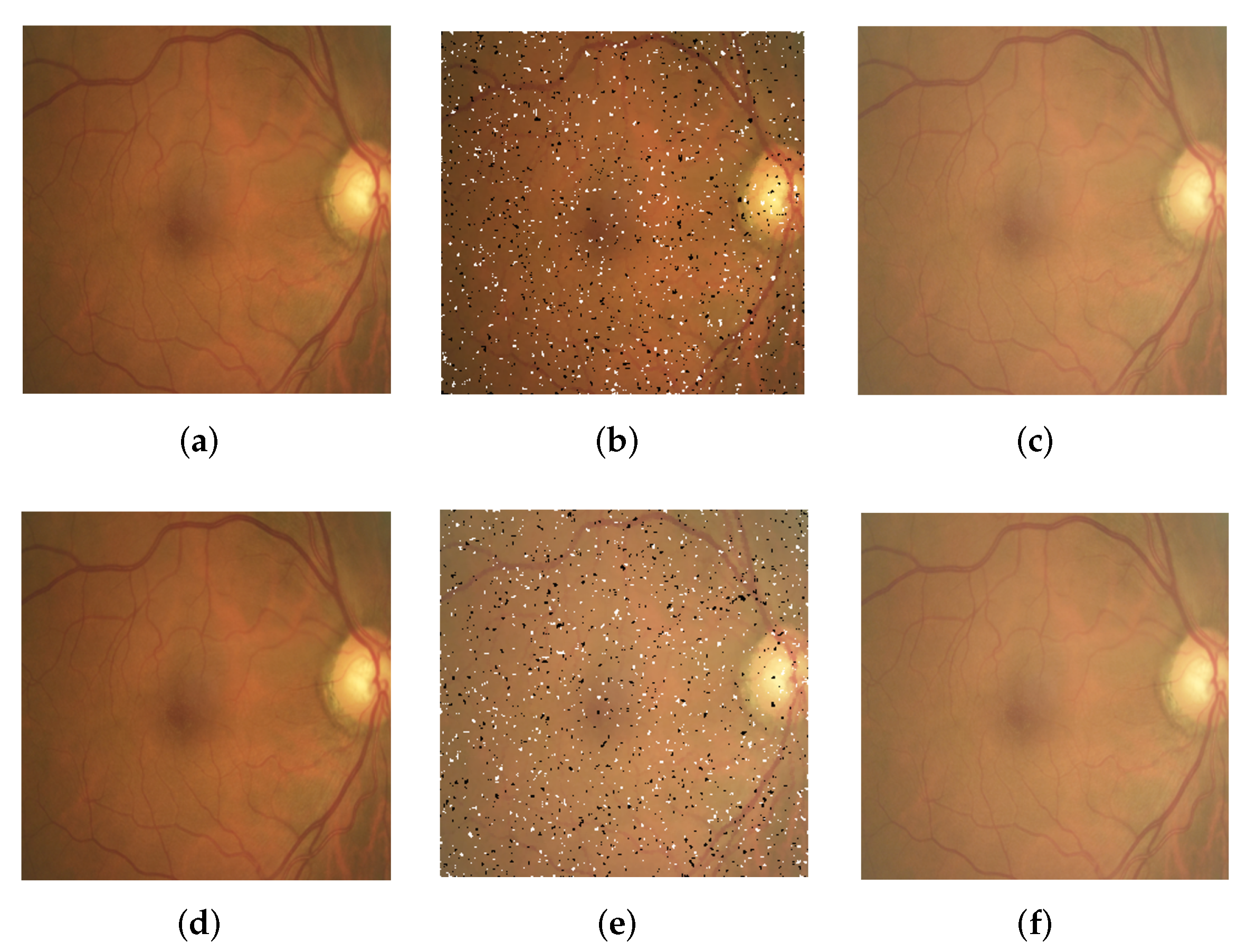
In the second step, fundus images are pre-processed with three filters and their combination, as shown in Figure 2, to augment and generalize fundus image data.

Table 3. Pre-processing methods.

Pre-Processing	Features
Salt & Pepper	It changes the pixel of an image to 0 or 255 with a certain probability. Instead of adding or reducing the value to the pixel value of the original image, the pixel exists in white or black with a specific probability.
Gamma correction	It corrects brightness by changing pixel values if the image is too dark or bright. The parameter is the gamma value $\gamma$. If $0<\gamma <1$, the image darkens; If $\gamma =1$, the image changes the same as the original image; if $\gamma <1$, the image brightens.
Remove noise	The median filter, one of the ways to remove noise, sorts the values of surrounding pixels and changes the pixel value to the median value. It is mainly used to remove salt and pepper.

summarizes the types and functions of pre-processing methods. Note that the pre-processing methods provided in this section are randomly applied to augment fundus images only for Classes 1 and 2.

Indeed, other pre-processing methods, such as shearing and shifting, may be helpful to improve the performance of the VA classifier. The image processing methods, such as shearing and shifting, that adjust the shape of images and the position of image features do not work effectively to improve the classification accuracy of our trained machines. For example, the shearing filter is not effective enough to improve the classification accuracy of VA measurement in our experiments. It seems that, when a CNN is trained, tweaking of the shape and shifting of the image location impair the shape of macular and optic nerve papilla that the human doctor observes carefully to check the health of the eye. Rotation of images is applied to augment fundus images from the datasets of Classes 1 and 2 which are much less than the other classes, and rescaling is limitedly applied fitting to our needs and purposes, such as transfer learning and SVM training.

3.3. Data Augmentation

Table 4. The number of augmented datasets.

	Class 1	Class 2	Class 3	Class 4
Initial Number of fundus images	2501	3972	16,104	32,575
The number of augmented datasets	7109	7115	16,104	32,575

shows the size of datasets of each VA level for our machine learning. For Classes 3 and 4, we do not augment or pre-process the datasets of Classes 3 and 4. The datasets of Classes 1 and 2 are much less than those of Classes 3 and 4. For the reason, we augment them in the following ways: first, we randomly select around 2500 from the dataset of Class 2 to make it balanced with the dataset of Class 1. Then, the two datasets of Classes 1 and 2 are augmented in the following way: the images of Classes 1 and 2 at the rate of 45% to 50% are randomly selected and rotated at −10${}^{\circ }$ to 10${}^{\circ }$. Then, 25% to 30% images of the rotated images of Classes 1 and 2 are applied for the filtering methods in Section 3.2. Then, the datasets of Classes 1 and 2 are augmented the following way: the images of Classes 1 and 2 are selected from the original datasets randomly at the rate of 45% to 50% and rotated at −10${}^{\circ }$ to 10${}^{\circ }$. Then, the filtering methods in Section 3.2 are applied for 25% to 30% images from the rotated images of Classes 1 and 2.

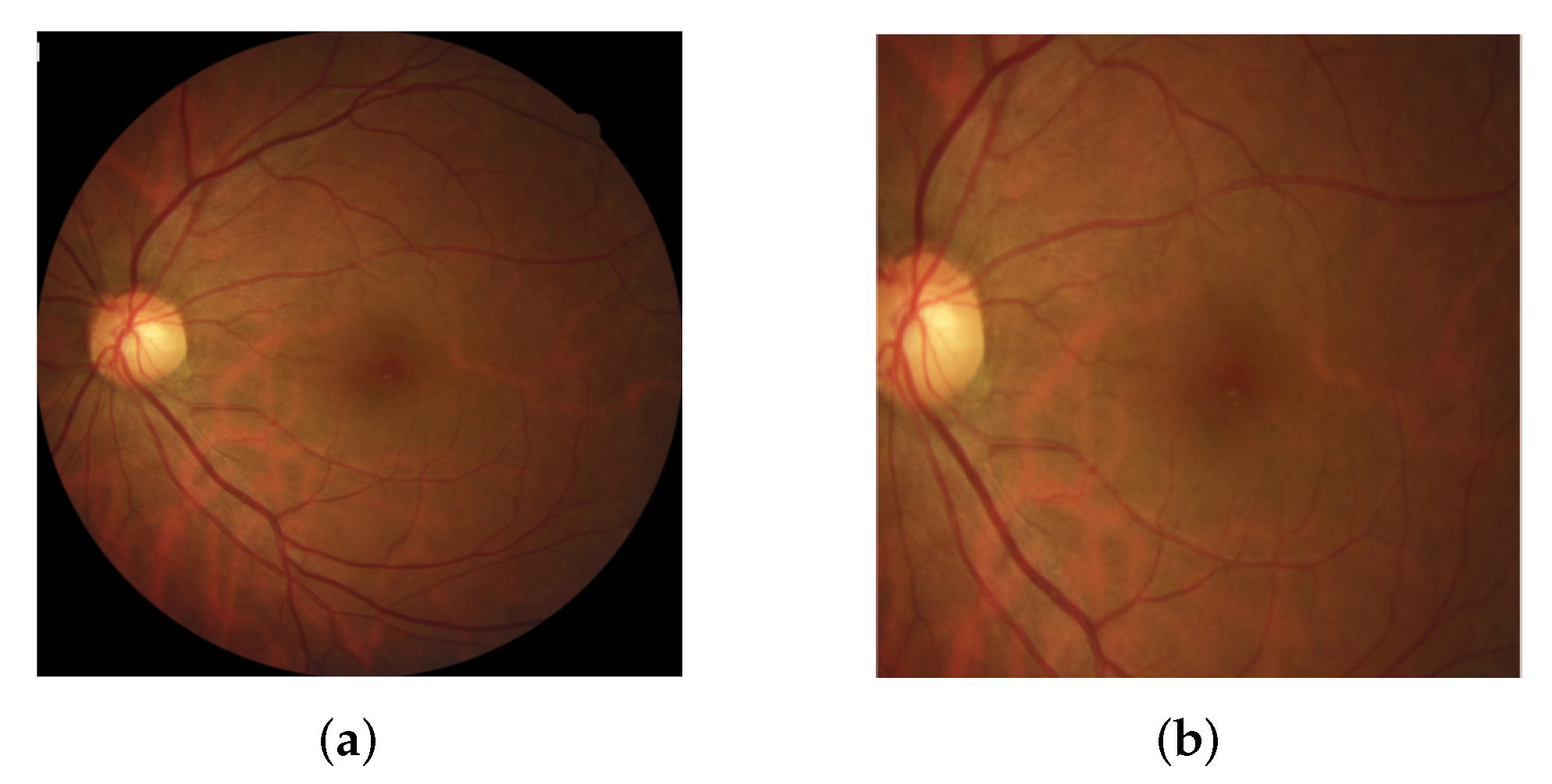
For all images of Classes 1 to 4, each image is cropped so that the main part of the macula and optic nerve papilla remains wholly highlighted, as shown in Figure 3, by completely removing the black part of each image. The original size of each image may not be identical to the others since they are captured in different fundus cameras. Thus, all images are resized in the size of 300 × 300.

Fundus images in all classes may be resized again for their individual methods when they are fed to CNN and SVM models for machine learning. For CNN models, the fundus images are resized into 244 × 244 fitting to the input image size of CNNs for transfer learning. For the SVM model, fundus images are resized into 32 × 32.

4. Deep Learning-Based Ensemble Method for VA Measurement

This study presents the measurement of VA based on only fundus images. The conventional 11 classes of the VA (0.0–1.0, step by 0.1) are grouped into four classes. We devise an ensemble method consisting of three machine learning models, two CNN models and one SVM model, to overcome the quantity unbalance of the fundus images and improve the accuracy of the VA classification.

4.1. Ensemble Methods

This section discusses the rationale for the use of Ensemble methods consisting of three machine learning techniques: two deep neural network (DNN) models using transfer learning of Convolution Neural Network (CNN) techniques based on VGG19 [28] and EfficientNet-B7 [29], and Support Vector Machine (SVM).

We applied each technique of VGG19, EfficientNet-B7, and SVM for the original fundus images for 4-level VA classification, and the accuracy of each model could not exceed about 70%. Even after augmenting fundus images, the accuracy of the VA classifier with individual machine learning models could not be more than about 80%. 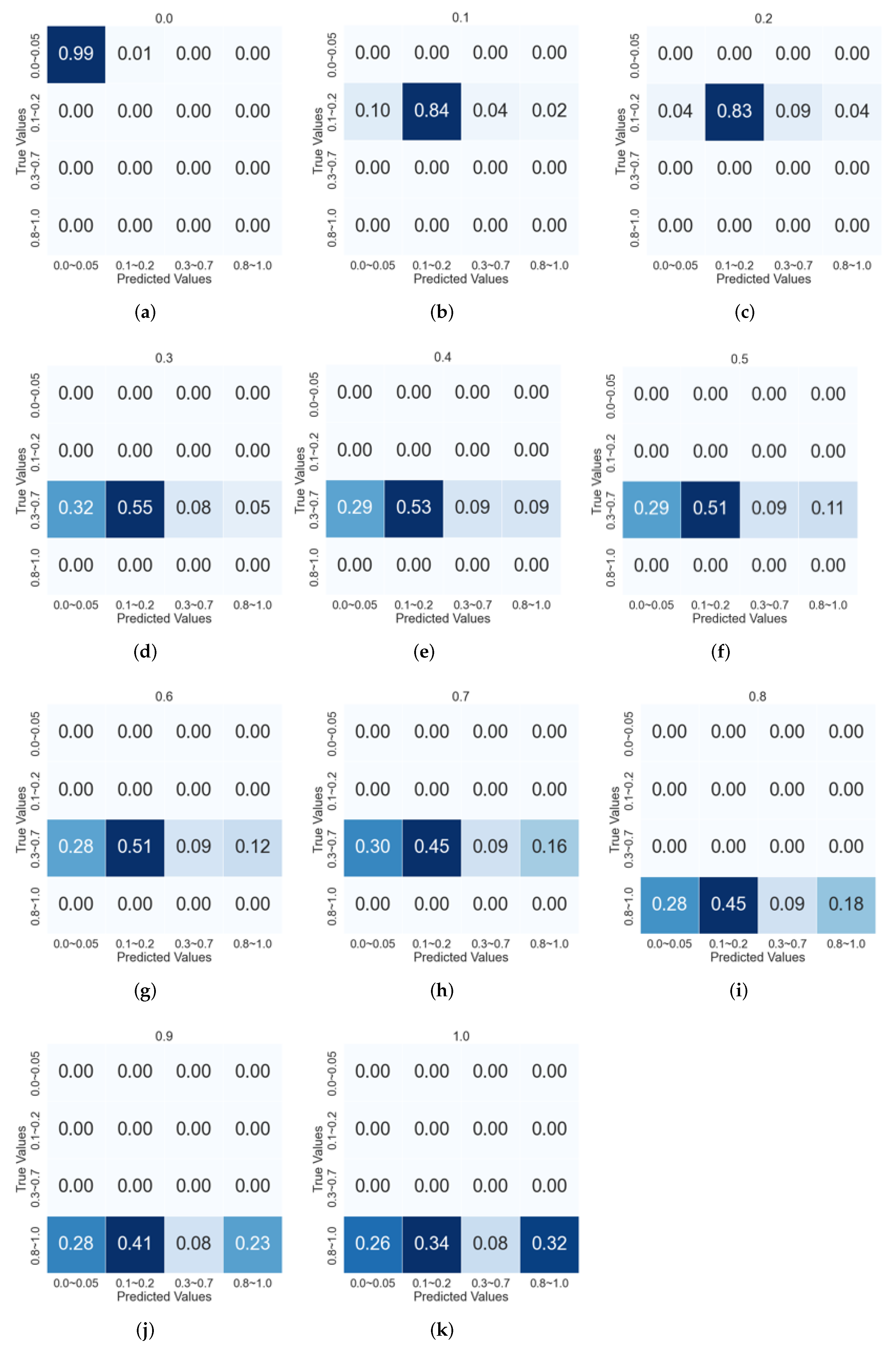To identify the cause of low accuracy of VA classification by each ML model, we analyzed confusion matrices in Figure 4 generated from the VGG-19 model.

Figure 4 shows the confusion matrix that the 4-level VA classifier based on VGG-19 returns when applied for each class of 11 VA levels. When the 4-level VA classifier is applied for Class-0.0 fundus images, the classification accuracy is 99% (Figure 4a). For Class-0.1 fundus images, the classifier makes 84% right decisions (Figure 4b). In the case of Class-0.4, only 53% of Class-0.3 fundus images are correctly classified (Figure 4e).

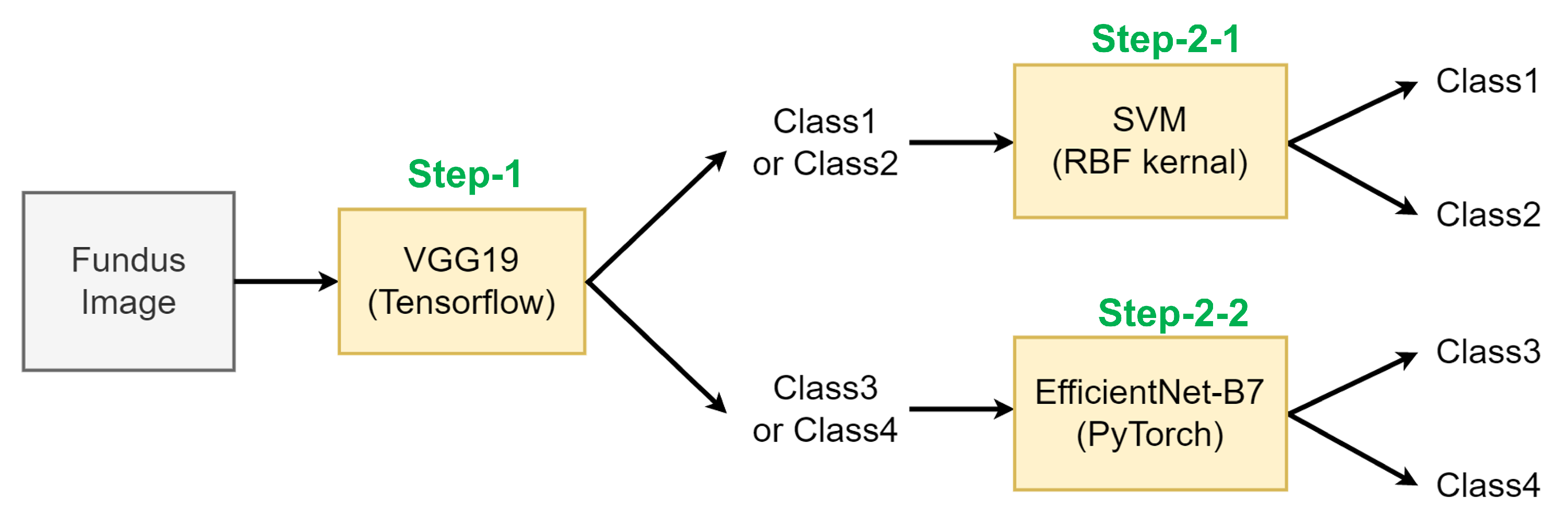
Based on our observation, we doubted that one of the main reasons for the misclassifications problem is the quantity unbalance between each class of the original datasets: The number of fundus images in Class 1 is 2501, 5% of the total datasets, while that of Class 4 is 32,575, accounting for 59% of the total datasets. To solve this problem, we propose an ensemble method, as shown in Figure 5. In this approach, a fundus image is classified in a hierarchical way, by different machine learning methods which perform the best classification performance at each classification step.

In the following, Classes 1 and 2 with a small number of fundus images are labeled as Class A, and Classes 3 and 4 with a large number of fundus images are labeled as Class B. Our method consists of three steps: In Step-1, a given fundus image is classified into either of Class A or Class B. In the following steps, the image classified into Class A is identified into either of Class 1 or Class 2 (Step-2-1), and the image in Class B is identified into either of Class 3 or Class 4 (Step-2-2).

We use three different ML models: VGG19-based CNN (implemented by Tensorflow), EfficientNet-B7-based CNN (implemented by PyTorch), and SVM-RBF-kernel [30].

Table 5. Classification accuracy when three machine learning models.

	4-Class Classification	Step-1	Step-2-1	Step-2-2
VGG19 (Tensorflow)	79%	94% 1	79%	78%
EfficientNet-B7 (PyTorch)	78%	92%	78%	79%
SVM (RBF kernel)	77%	91%	94%	79%

¹ This accuracy number is the highest in this step (column).

shows the VA classification accuracy of each ML model when those ML models perform each VA classification of 4-Class, Step-1, Step-2-1, and Step-2-2, respectively. We selected the highest accuracy technique for each stage and completed the entire model of fundus image’s VA classification machine learning based on these results.

In our ensemble method, a fundus image is first identified as either Class A (Classes 1 and 2) or Class B (Classes 3 and 4) by VGG19-based-CNN. The fundus image classified as Class A (Classes 1 and 2) at Step 1 is identified, at Step-2-1, as either Class 1 or Class 2 by the SVM-RBF-Kernel. Similarly, the image identified as Class B (Classes 3 and 4) is further identified as either Class 3 or Class 4 by EfficientNet-B7-based CNN on Step-2-2.

4.2. ML Models and Classification Performances

Transfer learning is a machine learning technique that adopts the weight values of the pre-trained model to another machine learning. It is practical, i.e., fast and accurate when the number of training data are small because it reuses the weights of the pre-trained model. The pre-trained models VGG19 and EfficientNet-B7 used in this paper have a Convolutional Neural Networks (CNN) structure for image classification. The CNN consists of a convolutional base that extracts image features and a classifier that identifies the class of images based on the extracted features. In our transfer learning using VGG19 and EfficientNet-B7 models, the convolutional base is reused without any modification, and the classifier layers are built by ourselves.

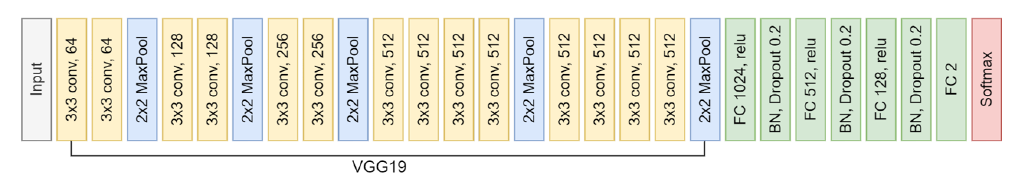
4.2.1. ML Model for Step-1: VGG19-Based CNN

The VGG19 model was developed to study how the depth of the network affects the classification outcomes, such as accuracy and training speed. The convolutional base of the VGG19 consisting of the convolution and pooling is composed of 19 layers. All convolution layers are characterized by fewer parameters, using filters of $3\times 3$. As a result, it can effectively extract features of images with small parameters, which leads to securing nonlinearity that can flexibly classify images. For Step-1, we build a VGG19 CNN model in which the convolutional base for feature extraction is based on VGG19 by transfer learning and the classification layers for the actual classification is built by ourselves, as shown in Figure 6.

Table 6. Learning parameters for VGG19 and EfficientNet-B7.

	Optimizer	Learning Rate	Batch Size	Epoch
VGG19 CNN	Adam	0.00002	128	500
EfficientNet-B7	Adam	0.00002	128	1000

shows the parameters we use to train DNN of VGG19 and EfficientNet-B7. We use a try-and-error approach to select the hyper-parameters after many experiments.

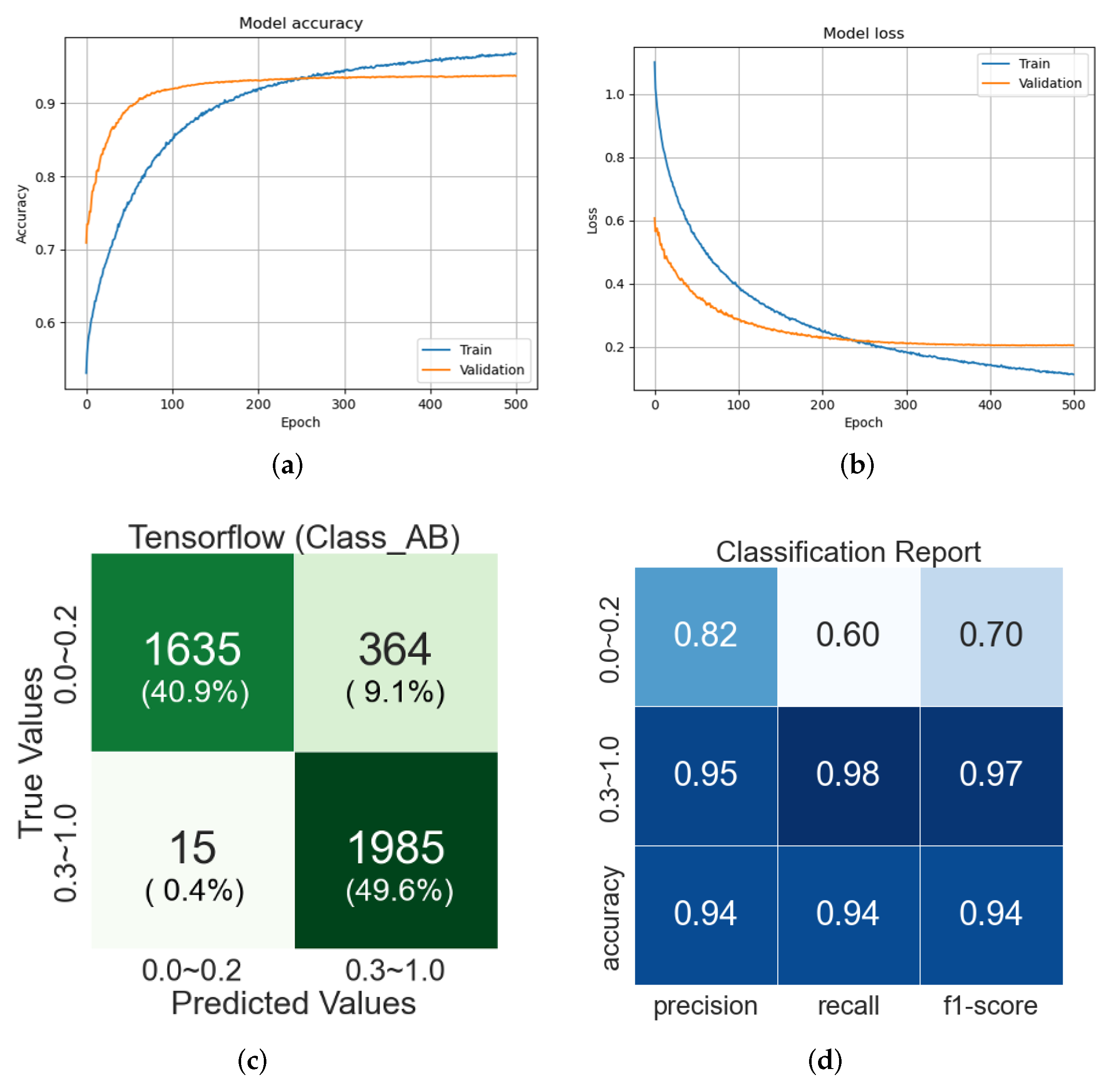
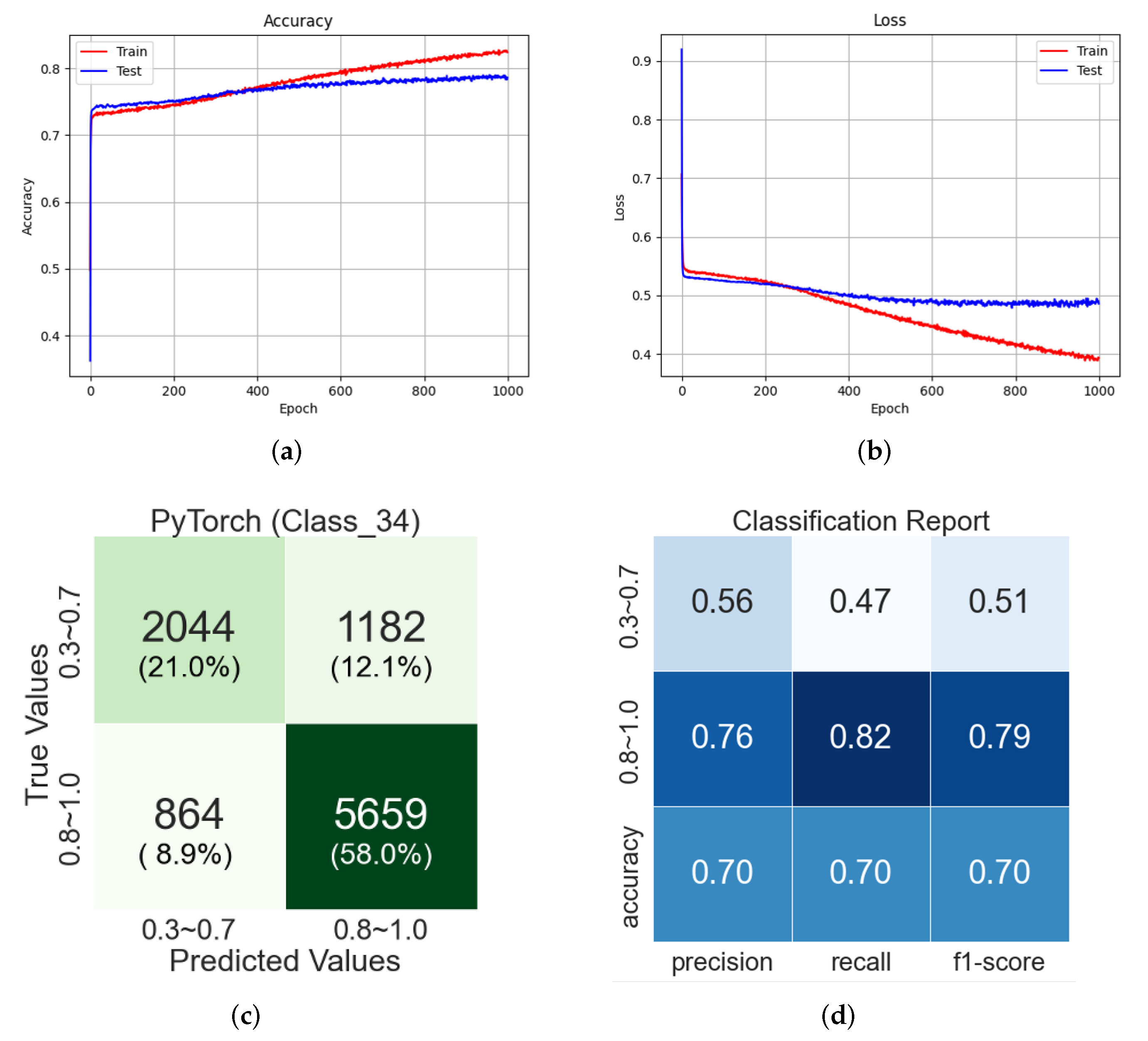
Figure 7a,b show the accuracy and loss changes of classifications during training and testing of the VGG19-based CNN model. Figure 7c shows a confusion matrix for 4000 images consisting of 1000 randomly selected from each class (Classes 1 to 4) of the original datasets, not augmented ones. The testing of VGG19-based CNN obtains 93% of the classification accuracy. From this confusion matrix, it is observed that some of Class A are identified as Class B. The reason might be inferred through the classification report in Figure 7d: The precision, which is the ratio of the data that is a true positive of the data determined to be positive, shows an accuracy of more than 80% in both Classes A and B. On the other hand, the recall, the ratio of positive data among the true positive data, is 60% for Class A compared to 98% for Class B. We believe that it is because of the data imbalance problem of the original datasets, thus the training of the VGG19 model is biased to Class B with a higher number of images. However, according to the f1-score in Figure 7d, which is the weight harmonic average of precision and recall and mainly used for unbalanced datasets, it can be inferred that the overall learning is well done because Class A shows the high accuracy of 70%.

4.2.2. ML Model for Step-2-1: SVM (RBF Kernel)

SVM is an algorithm based on statistical learning theory. It was initially devised to solve binary classification and regression analysis problems and extended for multiple classifications later. In addition, since the nonlinear separation between classes has been possible to solve using the notion of kernel method [31], it is popularly being used for data mining, artificial intelligence, prediction, and medical diagnosis.

In SVM, the learning data in a multidimensional space is expressed by:

$$\begin{array}{c}\hfill \{x_i,y_i\},i=1,...,n,y_i\in \{+1,-1\}\end{array}$$

(1)

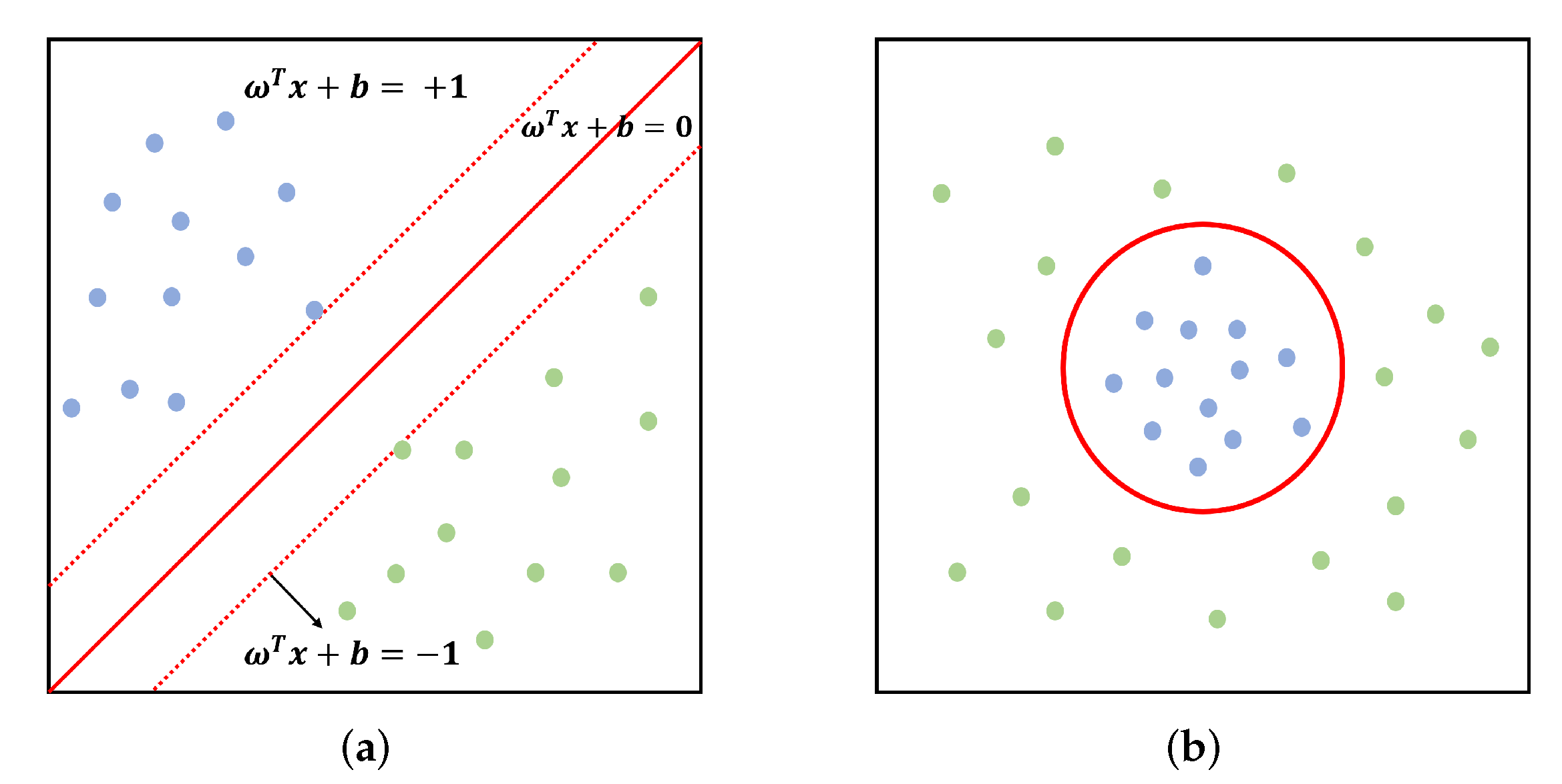
where $x_i$ is a set of data and $y_i$ is a label of $x_i$. For such learning data, several hyperplanes that separate the two classes can exist, but only one optimal hyperplane exists as shown in Figure 8a.

Such an optimal hyperplane maximizes the distance between the data closest to the hyperplane separated among each class of data. A hyperplane is defined by:

$$\begin{array}{c}\hfill {\omega }^T·x+b=0\end{array}$$

(2)

If data are linearly separable as shown in Figure 8a, the hyperplane that separates the two classes can be defined by Equation (3):

$$\begin{array}{c}\hfill \forall i,y_i({\omega }^T·x_i+b)-1\ge 0\end{array}$$

(3)

where $\omega$ is a vector of weight.

The training data for these two hyperplanes is called a support vector. In addition, since the margin between two hyperplanes must be maximized to obtain the hyperplanes of two classes, it becomes an optimization problem like the following objective of Equation (4) under Equation (3) as a constraint:

$$\begin{array}{c}\hfill min\{\frac{1}{2}||\omega |{|}^2\}\end{array}$$

(4)

In most cases, the data do not satisfy the above constraint because they are not linearly separable, as shown in Figure 8b. To solve this problem, the constraint is extended with a slack variable $\xi$ representing the distance from the hyperplane to misplaced data, and the objective is extended with a penalty term c. As a result, we obtain an optimization problem as follows:

$$\begin{array}{ccc}\hfill objective& :& min\{\frac{1}{2}||\omega |{|}^2+c\sum _{i=1}^n{\xi }_i\}\hfill \end{array}$$

(5)

$$\begin{array}{ccc}\hfill s.t& :& y_i({\omega }^T·x_i+b)>1-{\xi }_i\hfill \end{array}$$

(6)

For nonlinear data, a hyperplane of data having a nonlinear boundary can be obtained by data space transformation using $K(x_i,x_j)$ (Kernel function) for the features of data $x_i$ and $x_j$. The representative $K(x_j,x_j)$ is defined by, respectively:

• Polynomial (Inhomogeneous): $K(\overrightarrow{x_i},\overrightarrow{x_j})={(\overrightarrow{x_i}·\overrightarrow{x_j}+r)}^d$;
• Radial basis function: $K(\overrightarrow{x_i},\overrightarrow{x_j})=exp(-\frac{\left|\right|\overrightarrow{x_i}-\overrightarrow{x_j}{\left|\right|}^2}{2{\sigma }^2})$;
• Sigmoid function: $K(\overrightarrow{x_i},\overrightarrow{x_j})=tanh(\kappa \overrightarrow{x_i}·\overrightarrow{x_j}+c)$ for some (not every) $\kappa >0$ and $c<0$, where $\kappa$ is a gradient and c is a bias term (intercept).

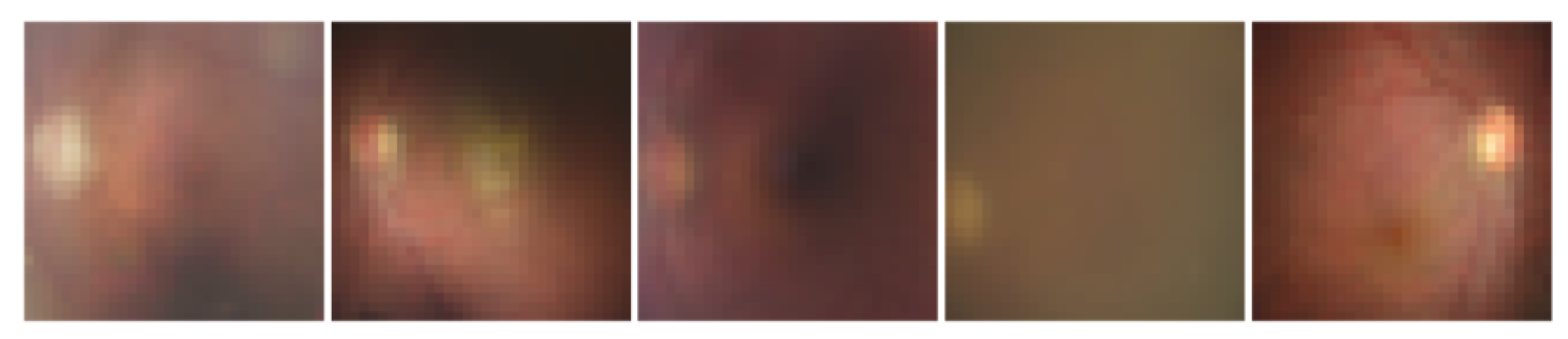
Now, the SVM model using RBF kernel that we used for Step-2-1 is explained. First, we resize all the images from $300\times 300\times 3$ to $32\times 32\times 3$, as shown in Figure 9, which shows the data shape and features that SVM-RBF-Kernel would use to reason the class of a fundus image.

Using the SVM class in the scikit-learn and the resized dataset above, the SVM-RBF-Kernel model is trained by varying kernel functions, c that determines how much error the model tolerates, and $\gamma$ that determines how flexible the hyperplane is set. In this study, we select the SVM model using the RBF kernel and train the model by setting $\gamma$ to 0.1 and increasing c from 1 to 100 by 20. 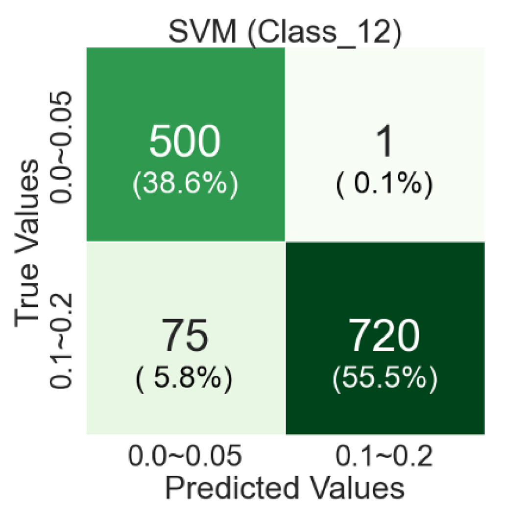The confusion matrix from the testing of SVM-RBF-Kernel model is shown in Figure 10.

In the confusion matrix from testing of an SVM-RBF-Kernel, the classification accuracy is about 58% for Class 1 and about 38% for Class 2, so the overall classification accuracy is about 96%. There are more Class 1 misclassified images than Class 2 misclassified images. The reason might be that there are similar abnormalities such as picture blurring or macular pigmentation and depigmentation in Class 2 as in Class 1.

4.2.3. ML Model for Step-2-2: EfficientNet-B7

EfficientNet is a state-of-the-art model with the best performance with a few parameters about image classification. The scaling-up method is often utilized to improve the performance of CNN. For scaling-up, one can increase the number of layers, the number of channels, or the input image’s resolution. EfficientNet finds the optimal combination of the above three scaling-up methods through AutoML (Automated Machine Learning) by uniformly adjusting the three methods using compound coefficients.

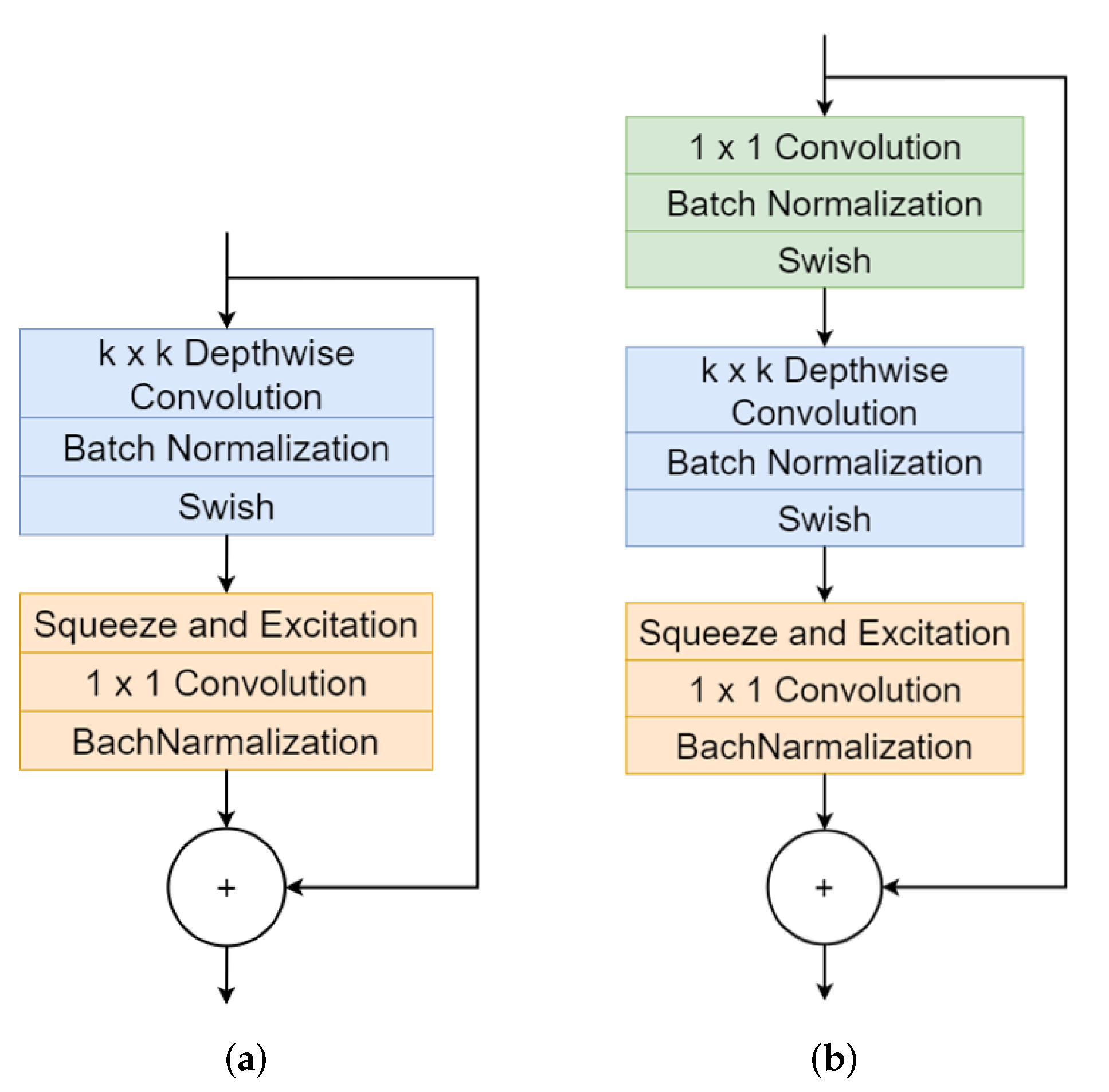
EfficientNet is composed of MBConv structured as shown in Figure 11. The MBConv expands the channel through 1 × 1 convolution operation and performs a Depthwise convolution operation that performs a convolution operation on each image channel. Depthwise convolution performs a convolution operation with $k\times k$ kernel for each channel of images. Each channel operated by Depthwise convolution becomes a feature map. Each layer uses batch normalization and then goes through the Swish function as an activation function. The Swish function prevents the gradient value from being saturated near zero during learning, unlike the Sigmoid and Tanh functions. In addition, unlike Relu, the Swish is less sensitive to the initial value and learning rate. For an enormous negative value, the Swish function returns a value of 0, but it preserves the value to some extent for a small negative value. Squeeze and Excitation Layer is composed of Global Average Pooling-Fully Connected Layer-ReLU-Fully Connected Layer-Sigmoid. The two Fully Connected Layers prevent the number of parameters from increasing with a bottle-neck structure. Each channel’s relative importance can be known through two Fully Connected Layers and nonlinear activation functions (ReLU, Sigmoid). The extracted map can be multiplied by a feature map that skips the Squeeze and Excitation Layer to highlight important features. Finally, the channel is reduced by the $1\times 1$ convolution operation. For channels reduced to $1\times 1$, using the activation function deletes sensitive information and it is less likely that sensitive information exists on other channels. Therefore, only batch normalization is used. In this way, the skip-connected input value is concatenated to the output value passed through multiple layers. This concatenation can preserve the previously learned information, learn additionally from it, and reduce memory usage.

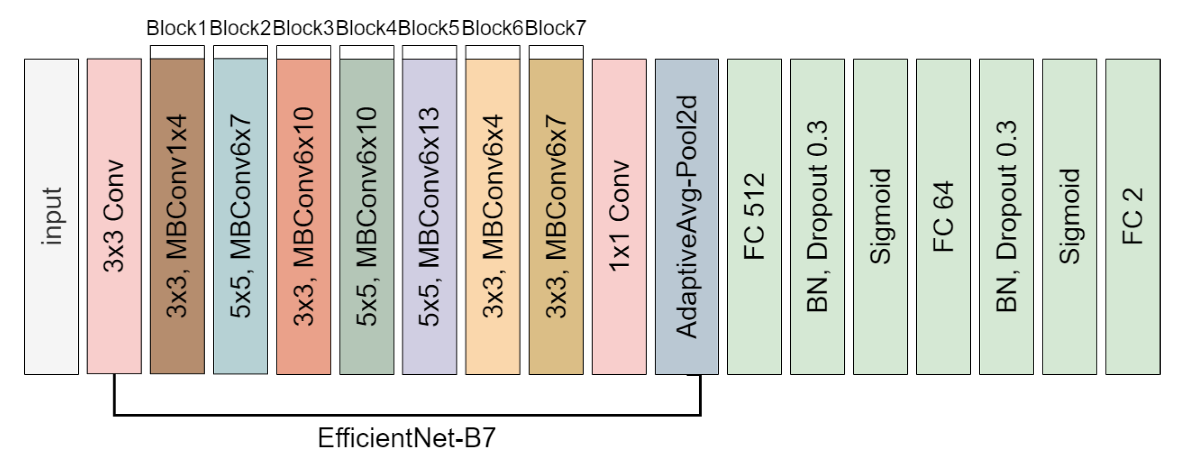
The EfficientNet-B7 model uses fewer parameters and provides the best performance among various EfficientNet models. As shown in Figure 12, the final model we apply for the VA classification in Step-2-2 is completed by transfer learning, in which the convolutional base for feature extraction is reused and the classifier part is directly built by ourselves.

The parameters we used to train CNN based on EfficientNet-B7 are also given in Table 6.

In Figure 13a, the classification accuracy of testing data are about 79%, and in Figure 13b, the loss of testing data continues to drop, but the change of the loss value is insignificant after epoch 300. The confusion matrix in Figure 13c is computed with 20% of each class data randomly selected from the original datasets. In the classification report in Figure 13d, the f1-score of Class 3 (Class 0.3–0.7) is 0.51 and that of Class 4 (Class 0.8–1.0) is 0.79. The total f1-score is 0.70. The training of EfficientNet-B7-based CNN seems biased to Class 4, due to the imbalance of the data quantity, but the overall f1-score of the EfficientNet-B7-based CNN shows that the training of the CNN model is well done.

5. Results

In this section, we present the experiment results where the 4-Class VA classifier in Figure 5 is applied for the validation datasets of the patient’s fundus image and VA information. To figure out the accuracy of the overall model, we selected 1000 fundus images with patient VA information for each class from the original datasets and conducted a classification experiment. The selected fundus images are not pre-processed with any filter.

5.1. Validation of Classification of VGG19-Based CNN for Step-1

First, the VA classifier for Step-1 where Classes A and B are identified was tested by using VGG19-based CNN, and the confusion matrix is as shown in Figure 14.

The classification between Classes A and B is performed by VGG19-based CNN, of which the classification accuracy is around 94% as shown in Table 5. Our 4-Class VA classifier at Step-1 adopts the VGG19-based CNN, thus it cannot outperform the classification accuracy of VGG19-based CNN for VA classification.

In Figure 14a, the images in Class A are more misclassified than those in Class B. It is in accordance with the fact that the recall of Class A is 60% in Figure 7d. We investigated the probability value of Softmax of images misclassified in the confusion matrix and the characteristics of these images. In Table 2, the images in Class A look generally blurred and partially poorly observed. On the other hand, the images in Class B look relatively cleaner than Class A, and the macula and optic disc are clearly observable. However, the misclassified images of Class A in this experiment have the more observable optic disc and macula images than the images of Class A Table 2.

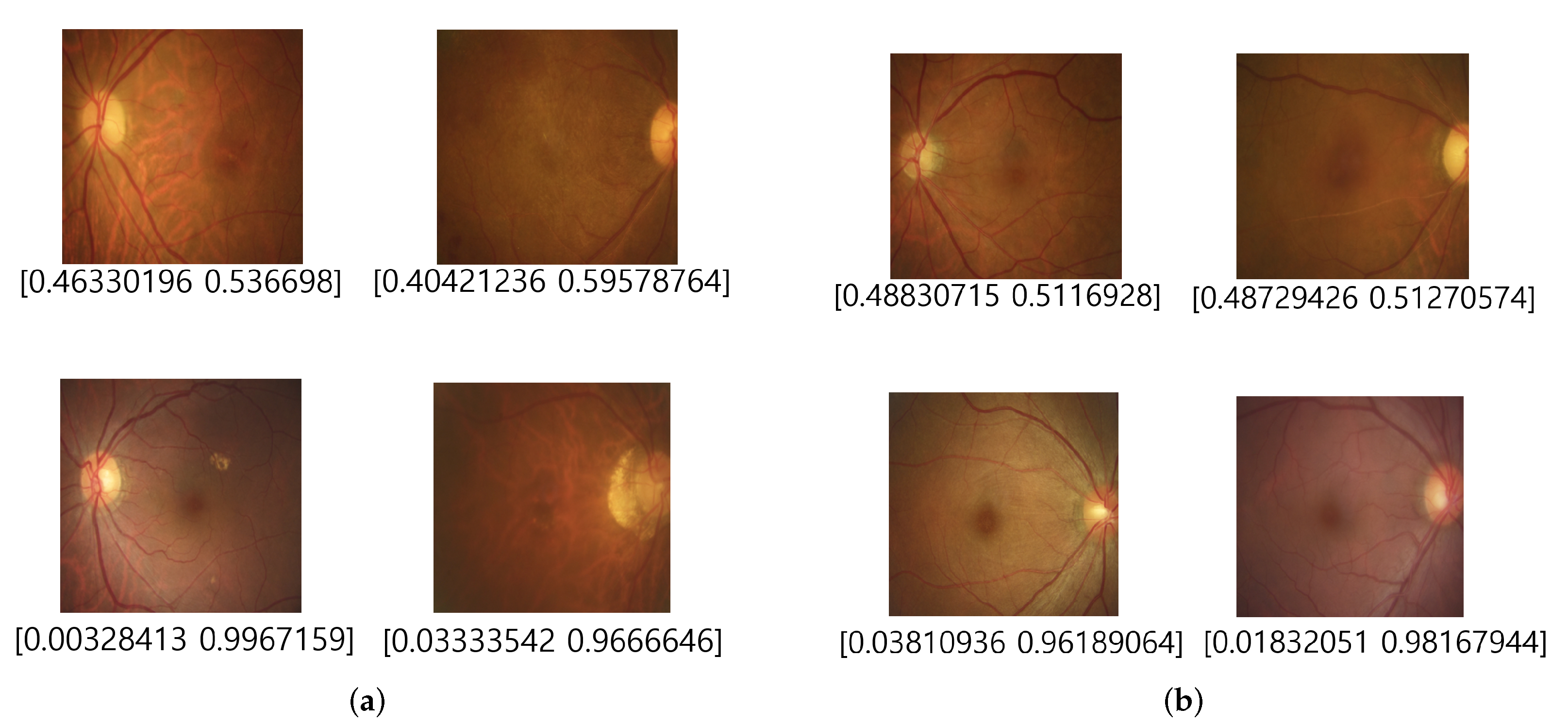
Figure 15 shows some misclassification examples where the fundus images in Class 1 or Class 2 of Class A are misclassified as Class B. Note that the decision probability of Softmax of the fundus images in the first line is both close to 50%, and that means that they can likely be misclassified. Furthermore, the macular in fundus images in the second line look cleaner, in contrast to those in Table 2.

For the misclassification cases of Class B, the misclassified images in Class B look very blurred or macularly unclear, as shown in Figure 16.

5.2. Validation of Classification of SVM-RBF-Kernel ML for Step-2-1

The fundus images of Class A identified in Step-1 by VGG19-based CNN are checked if it is in either Class 1 (0.0–0.05) or Class 2 (0.1–0.2) by using the SVM-RBF-Kernel.

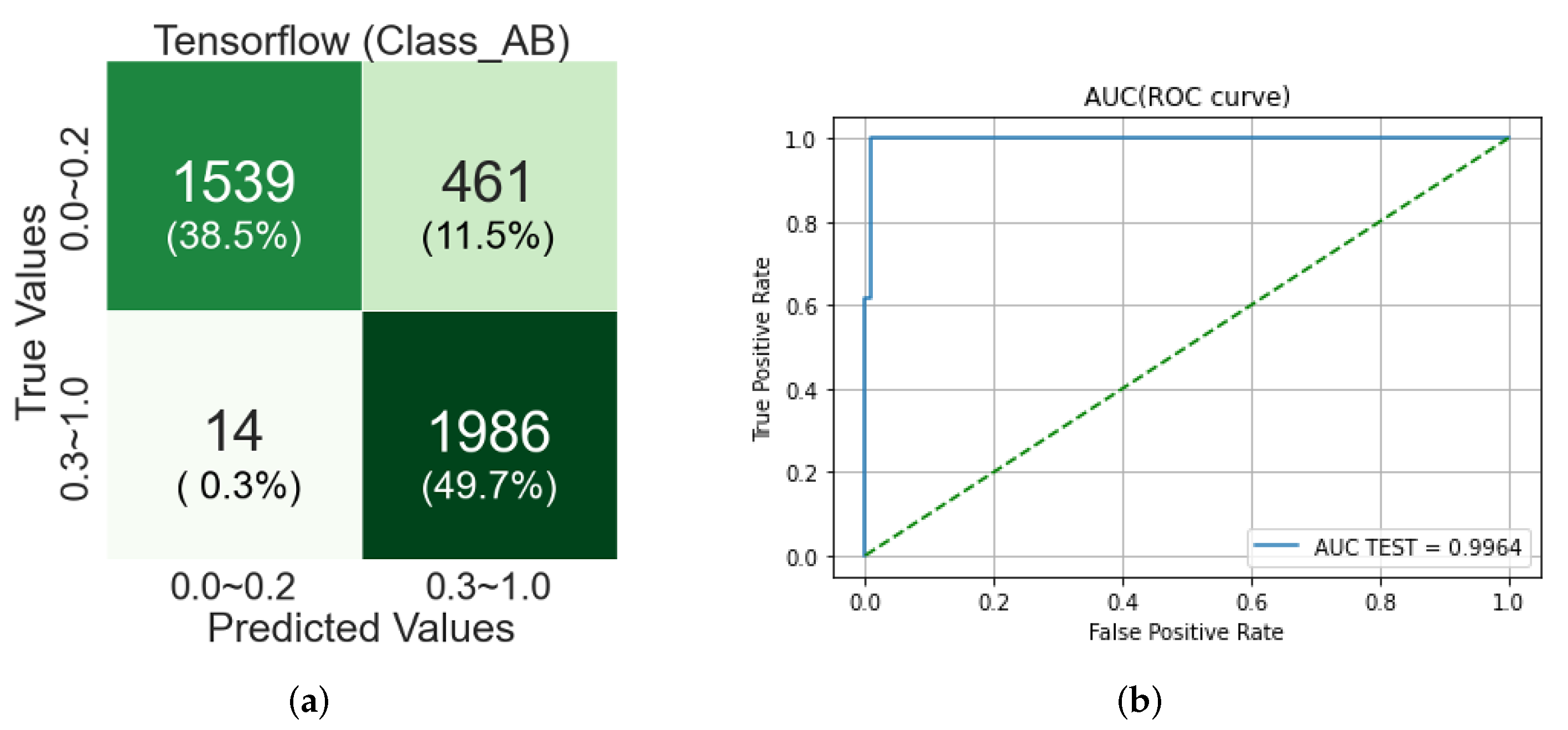
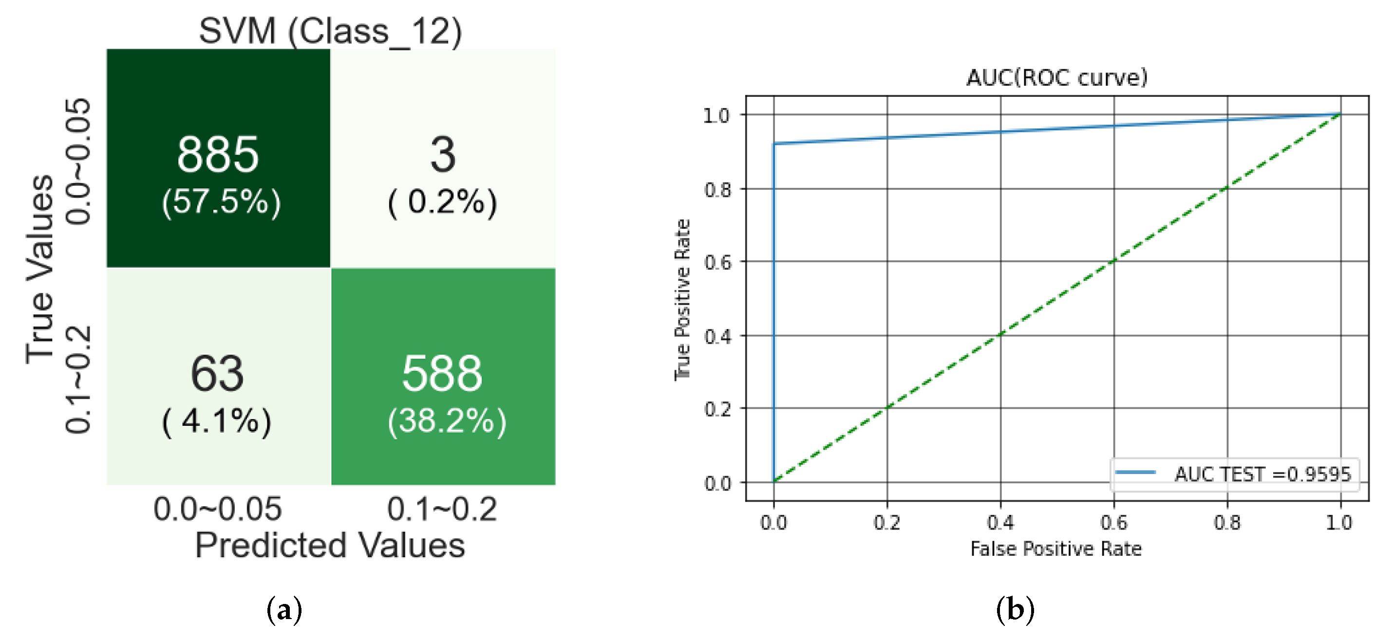
Figure 17 shows a confusion matrix, and AUC score and ROC curve. In the confusion matrix, the classification accuracy for Classes 1 and 2 is about 58% and 38%, respectively, and the overall classification accuracy is about 96%.

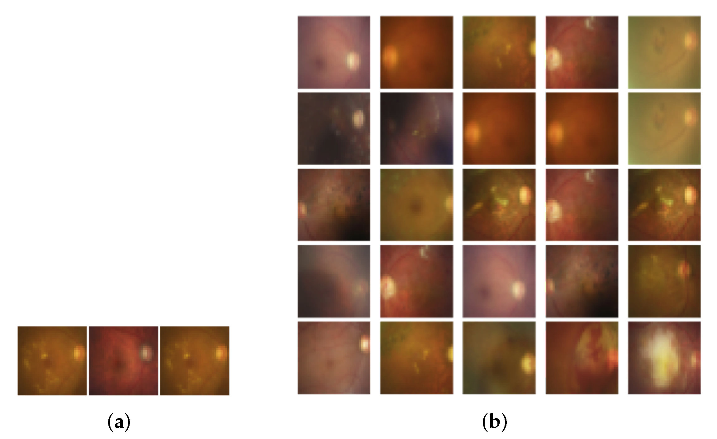
Tbltbl:fp-cls-features shows the images that should be classified as Class 1 but misclassified as Class 2 or vice versa: The misclassified fundus images of Class 1 (0.0–0.05) are cloudy, and each part of the fundus images is not easily identified. In addition, abnormal findings such as pigmentation and depigmentation of the macula are shown. On the other hand, Class 2 has fewer hazy fundus images and fewer abnormal findings such as macular pigmentation and depigmentation than Class 1.

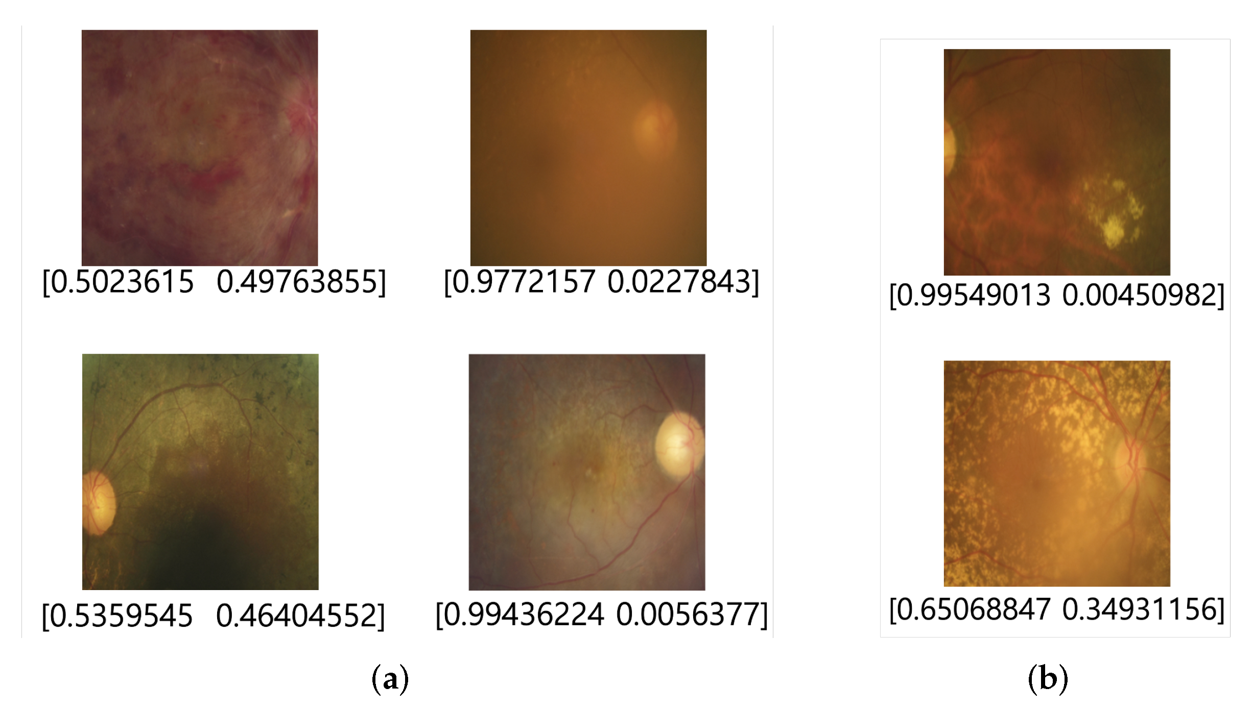
In this validation, as shown in Figure 18, the fundus images of Class 1 misclassified as Class 2 are relatively clearer and have fewer abnormalities, such as pigmentation and depigmentation in the macula, than images classified correctly. The fundus Images of Class 2 misclassified as Class 1 look more blurred than images classified correctly, and the abnormalities, such as pigmentation and depigmentation, in the macula, appear more severe.

5.3. Validation of Classification of EfficientNet-B7-Based CNN for Step-2-2

For the fundus images identified as Class B in the previous step, EfficientNet-B7-based CNN identifies the individual classes as either Class 1 or Class 2.

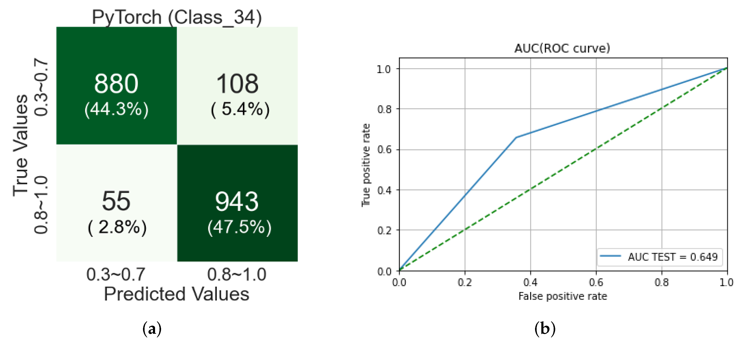
Figure 19 shows a confusion matrix and AUC score and ROC curve from the validation of the classification by EfficientNet-B7-based CNN in Step-2-2. In the confusion matrix, the classification accuracy for Classes 3 and 4 is about 44% and 48%, respectively, so the overall classification accuracy is 92%.

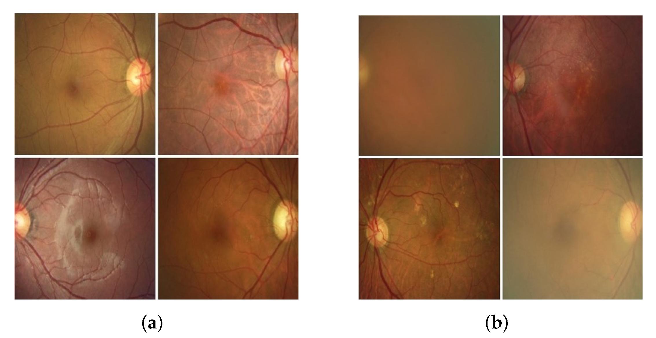
In Table 2, the optic disc and macula of the fundus images in Class 3 look clean and have no pigment abnormality or bleeding. On the other hand, the fundus images in Class 3 are an overall blurry image compared to Class 4. In the misclassification case of Class 3, the fundus images, as shown in Figure 20a, have the optic disc and macula in clearer. Meanwhile, in the misclassification case of Class 4, the optic disc and macula in the fundus image are not clearly observed, and a lot of blurred images are observed.

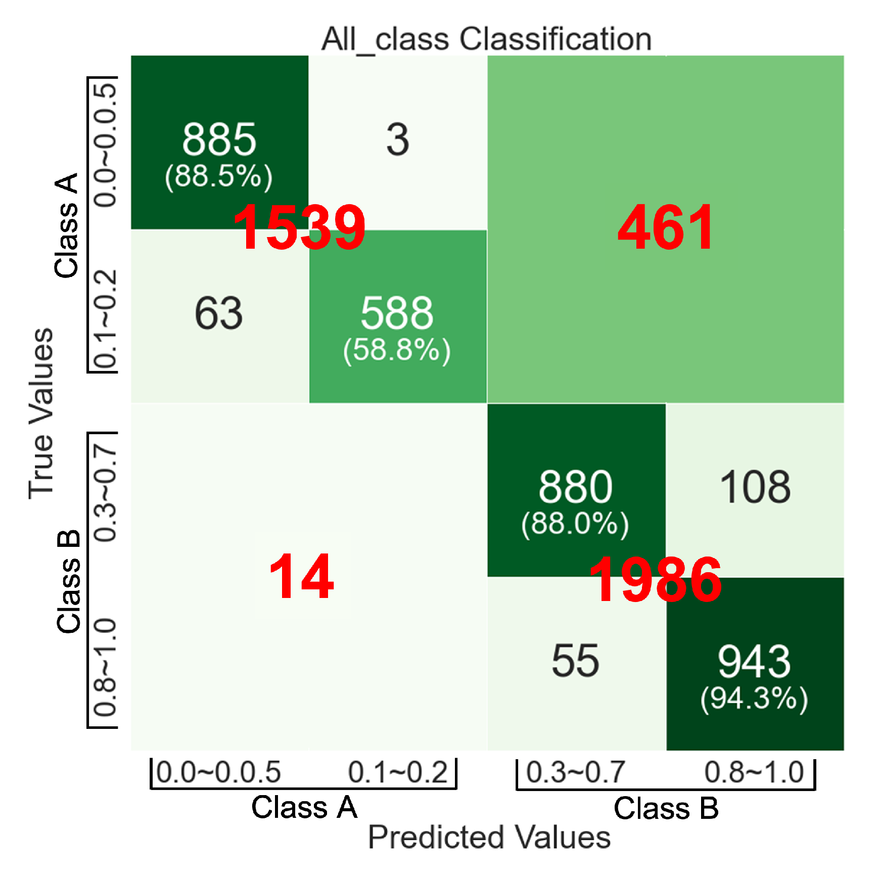
The conclusion about the classification accuracy of the 4-Class VA Classifier using fundus images is as follows: We randomly selected 1000 for each class and tested the classifier with a total of 4000 fundus images and the relevant patient’s VA information. Figure 21 is a confusion matrix for the classification accuracy of the entire model based on the ensemble method. It combines Figure 14a, Figure 17a and Figure 19a and summarizes the classification performance of the 4-Class VA classifier. This confusion matrix consists of two types of quadrants: big quadrants and small quadrants. The big quadrants include the classification accuracy rate for Classes A and B performed at Step-1. The small quadrants include the classification accuracy rate for Classes 1–4 performed at Step-2. Notice the numbers on the diagonal in this confusion matrix, starting at the top left and flowing down to the right. These numbers are the classification accuracy for 1000 fundus images from each class from Class 1 to Class 4. It says that the classification accuracy of our approach to VA measurement based on fundus images are 88.5%, 58.8%, 88.0% and 94.3% for each classification of Class 1 to Class 4, respectively. We can say that the classification accuracy of the 4-Class VA classifier is 82.4% on average.

Table 7. Comparison of VA classifiers’ performance based on our ensemble method and VGG-19.

VA Classes	Ensemble Method				VGG-19
	Average Accuracy	Class Accuracy	Sensitivity	Specificity	Average Accuracy	Class Accuracy	Sensitivity	Specificity
1	82.4%	88.5%	0.885	0.038	78%	0.89	0.988	0.0042
2		58.8%	0.588	0.121		0.8	0.832	0.06
3		88.0%	0.88	0.04		0.69	0.563	0.137
4		94.3%	0.943%	0.024		0.74	0.764	0.079

shows the comparison between the performance of VA classifiers based on our ensemble method and VGG-19 in terms of four aspects: the overall average accuracy, each class accuracy, sensitivity, and specificity. The reason why VGG-19 is selected to compare against our ensemble method is that it shows the best performance of VA classification as shown in Table 5. It shows that our ensemble method outperforms the VGG-19 VA classifier in the overall accuracy, but the VGG-19 VA classifier shows higher accuracy in VA- classification for Class-2 than our ensemble method. From the aspects of sensitivity and specificity, they are not comparable because one of them does not outperform the other in all classes.

6. Conclusions

Visual sight is one of the most sensing capabilities of humans. Visual Acuity (VA) is a fundamental measure of the ability of the eye to distinguish shapes and the details of objects at a given distance. It is a primary indicator of eye health and the results of medical treatment for eye diseases. VA is typically measured using VA measuring tools, such as Snellen or E-Chart. In particular, communication with the tester is essential. However, it is not suitable or impossible to use the classical ways of measuring VA for patients under mobility difficulties, unconscious states, or lack of cooperation, and an infant or very young patient.

To solve those problems, we present an ensemble method based on machine learning based on fundus images and VA information of patients. Fundus photography is one of the most popularly used photo images for an eye examination and rarely needs the cooperation of patients to obtain the image. In our approach, 11 classes in classical VA measurement are abstracted into four classes, Classes 1–4, to overcome the discrepancy problem of fundus image data quantity for each of 11 classes.

In the ensemble method, the VA is measured in two steps: In the first step, Classes 1–2 and Classes 3–4 are classified as either Class A or Class B. In the second step, the fundus images in Class A is classified as either Class 1 or Class 2 and those in Class B is classified as either Class 3 or Class 4.

We use three different machine learning techniques for each classification: VGG-19- base CNN, EfficientNet-B7-based CNN, and SVM-RBF-Kernel. We evaluated the three techniques for each classification of individual steps and selected one of them that shows the best classification performance for each step. From our validation of the 4-Class VA classifier using 4000 fundus images from each of the four classes, we obtained 88.5%, 58.8%, 88 %, and 94.3% of classification accuracy for each level of four classes, respectively, and the classification accuracy of 82.4% on average.

To make our approach useful in practice, we have more challenges to overcome. For example, the density of the background pigmentation of the fundus oculi is dependent on race. We need to obtain more data from other countries and races to overcome this problem. In addition, the examinee’s subjectivity in measuring vision acuity may degrade the collected data quality. In addition, the fundus image shows the functional status of the eye, thus measuring visual acuity with only fundus images have limitations since our vision depends on both the function of the eye and the function of the brain.

References

- Bourne, R.R.A.; Adelson, J.; Flaxman, S.; Briant, P.; Bottone, M.; Vos, T.; Naidoo, K.; Braithwaite, T.; Cicinelli, M.; Jonas, J.; et al. Global Prevalence of Blindness and Distance and Near Vision Impairment in 2020: Progress towards the Vision 2020 Targets and What the Future Holds. Available online: https://iovs.arvojournals.org/article.aspx?articleid=2767477 (accessed on 24 January 2022).
- Marsden, J.; Stevens, S.; Ebri, A. How to Measure Distance Visual Acuity. Available online: https://0-www-ncbi-nlm-nih-gov.brum.beds.ac.uk/pmc/articles/PMC4069781/ (accessed on 24 January 2022).
- Panwar, N.; Huang, P.; Lee, J.; Keane, P.A.; Chuan, T.S.; Richhariya, A.; Teoh, S.; Lim, T.H.; Agrawal, R. Fundus photography in the 21st century—A review of recent technological advances and their implications for worldwide healthcare. Telemed.-Health 2016, 22, 198–208. [Google Scholar] [CrossRef] [PubMed]
- Colenbrander, A. The historical evolution of visual acuity measurement. Vis. Impair. Res. 2008, 10, 57–66. [Google Scholar] [CrossRef]
- Bach, M. The Freiburg Visual Acuity Test-automatic measurement of visual acuity. Optom. Vis. Sci. 1996, 73, 49–53. [Google Scholar] [CrossRef] [PubMed]
- Brady, C.J.; Eghrari, A.O.; Labrique, A.B. Smartphone-based visual acuity measurement for screening and clinical assessment. JAMA 2015, 314, 2682–2683. [Google Scholar] [CrossRef]
- Tofigh, S.; Shortridge, E.; Elkeeb, A.; Godley, B. Effectiveness of a smartphone application for testing near visual acuity. Eye 2015, 29, 1464–1468. [Google Scholar] [CrossRef] [PubMed]
- Kononenko, I. Machine learning for medical diagnosis: History, state of the art and perspective. Artif. Intell. Med. 2001, 23, 89–109. [Google Scholar] [CrossRef] [Green Version]
- Foster, K.R.; Koprowski, R.; Skufca, J.D. Machine learning, medical diagnosis, and biomedical engineering research-commentary. Biomed. Eng. Online 2014, 13, 1–9. [Google Scholar] [CrossRef] [Green Version]
- Erickson, B.J.; Korfiatis, P.; Akkus, Z.; Kline, T.L. Machine learning for medical imaging. Radiographics 2017, 37, 505–515. [Google Scholar] [CrossRef]
- Willemink, M.J.; Koszek, W.A.; Hardell, C.; Wu, J.; Fleischmann, D.; Harvey, H.; Folio, L.R.; Summers, R.M.; Rubin, D.L.; Lungren, M.P. Preparing medical imaging data for machine learning. Radiology 2020, 295, 4–15. [Google Scholar] [CrossRef]
- Richens, J.G.; Lee, C.M.; Johri, S. Improving the accuracy of medical diagnosis with causal machine learning. Nat. Commun. 2020, 11, 1–9. [Google Scholar] [CrossRef]
- Zemblys, R.; Niehorster, D.C.; Komogortsev, O.; Holmqvist, K. Using machine learning to detect events in eye-tracking data. Behav. Res. Methods 2018, 50, 160–181. [Google Scholar] [CrossRef] [PubMed]
- Grewal, P.S.; Oloumi, F.; Rubin, U.; Tennant, M.T. Deep learning in ophthalmology: A review. Can. J. Ophthalmol. 2018, 53, 309–313. [Google Scholar] [CrossRef] [PubMed]
- Armstrong, G.W.; Lorch, A.C. A (eye): A review of current applications of artificial intelligence and machine learning in ophthalmology. Int. Ophthalmol. Clin. 2020, 60, 57–71. [Google Scholar] [CrossRef] [PubMed]
- Wang, Z.; Keane, P.A.; Chiang, M.; Cheung, C.Y.; Wong, T.Y.; Ting, D.S.W. Artificial intelligence and deep learning in ophthalmology. Artif. Intell. Med. 2020, 1–34. [Google Scholar] [CrossRef]
- Liu, T.A.; Ting, D.S.; Paul, H.Y.; Wei, J.; Zhu, H.; Subramanian, P.S.; Li, T.; Hui, F.K.; Hager, G.D.; Miller, N.R. Deep learning and transfer learning for optic disc laterality detection: Implications for machine learning in neuro-ophthalmology. J. Neuro-Ophthalmol. 2020, 40, 178–184. [Google Scholar] [CrossRef]
- Jais, F.N.; Che Azemin, M.Z.; Hilmi, M.R.; Mohd Tamrin, M.I.; Kamal, K.M. Postsurgery Classification of Best-Corrected Visual Acuity Changes Based on Pterygium Characteristics Using the Machine Learning Technique. Sci. World J. 2021, 2021, 6211006. [Google Scholar] [CrossRef]
- Ryu, H.; Ryu, H.S.; Wallraven, C. Analysis of Vision Acuity (VA) using Artificial Intelligence (AI): Comparison of Machine Learning Models and Proposition of an Optimized Model. J. Korea Soc. Vis. Sci. 2020, 22, 229–236. [Google Scholar] [CrossRef]
- Rohm, M.; Tresp, V.; Müller, M.; Kern, C.; Manakov, I.; Weiss, M.; Sim, D.A.; Priglinger, S.; Keane, P.A.; Kortuem, K. Predicting visual acuity by using machine learning in patients treated for neovascular age-related macular degeneration. Ophthalmology 2018, 125, 1028–1036. [Google Scholar] [CrossRef]
- Alexeeff, S.E.; Uong, S.; Liu, L.; Shorstein, N.H.; Carolan, J.; Amsden, L.B.; Herrinton, L.J. Development and Validation of Machine Learning Models: Electronic Health Record Data To Predict Visual Acuity After Cataract Surgery. Perm. J. 2020, 25, 25. [Google Scholar] [CrossRef]
- Li, H.; Chutatape, O. Fundus image features extraction. In Proceedings of the 22nd Annual International Conference of the IEEE Engineering in Medicine and Biology Society (Cat. No. 00CH37143), Chicago, IL, USA, 23–28 July 2000; Volume 4, pp. 3071–3073. [Google Scholar]
- Mateen, M.; Wen, J.; Song, S.; Huang, Z. Fundus image classification using VGG-19 architecture with PCA and SVD. Symmetry 2019, 11, 1. [Google Scholar] [CrossRef] [Green Version]
- Xu, K.; Feng, D.; Mi, H. Deep convolutional neural network-based early automated detection of diabetic retinopathy using fundus image. Molecules 2017, 22, 2054. [Google Scholar] [CrossRef] [PubMed] [Green Version]
- Cheng, X.; Feng, X.; Li, W. Research on Feature Extraction Method of Fundus Image Based on Deep Learning. In Proceedings of the 2020 IEEE 3rd International Conference on Automation, Electronics and Electrical Engineering (AUTEEE), Shenyang, China, 20–22 November 2020; pp. 443–447. [Google Scholar]
- Trucco, E.; Ruggeri, A.; Karnowski, T.; Giancardo, L.; Chaum, E.; Hubschman, J.P.; Al-Diri, B.; Cheung, C.Y.; Wong, D.; Abramoff, M.; et al. Validating retinal fundus image analysis algorithms: Issues and a proposal. Investig. Ophthalmol. Vis. Sci. 2013, 54, 3546–3559. [Google Scholar] [CrossRef] [PubMed] [Green Version]
- Ho, C.Y.; Pai, T.W.; Chang, H.T.; Chen, H.Y. An atomatic fundus image analysis system for clinical diagnosis of glaucoma. In Proceedings of the 2011 International Conference on Complex, Intelligent, and Software Intensive Systems, Seoul, Korea, 30 June–2 July 2011; pp. 559–564. [Google Scholar]
- Simonyan, K.; Zisserman, A. Very Deep Convolutional Networks for Large-Scale Image Recognition. arXiv 2015, arXiv:1409.1556. [Google Scholar]
- Tan, M.; Le, Q.V. EfficientNet: Rethinking Model Scaling for Convolutional Neural Networks. arXiv 2019, arXiv:1905.11946. [Google Scholar]
- Thurnhofer-Hemsi, K.; López-Rubio, E.; Molina-Cabello, M.A.; Najarian, K. Radial basis function kernel optimization for Support Vector Machine classifiers. arXiv 2020, arXiv:2007.08233. [Google Scholar]
- Scholkopf, B. The kernel trick for distances. In Advances in Neural Information Processing Systems; MIT Press: Cambridge, MA, USA, 2001; pp. 301–307. [Google Scholar]
Figure 1.
A normal fundus photograph of a right eye.
Figure 2.
Pre-processing of fundus images. (a) Original; (b) Salt and pepper; (c) Gamma correction; (d) Remove noise; (e) Gamma correction + Salt and pepper; and (f) Gamma correction + Remove noise.
Figure 3.
Before and after cropping fundus images. (a) before cropping; (b) after cropping.
Figure 4.
Confusion matrices from 4-Class VA Classifier’s classification results for 11 classes of fundus images. (a) Class-0.0; (b) Class-0.1; (c) Class-0.2; (d) Class-0.3; (e) Class-0.4; (f) Class-0.5; (g) Class-0.6; (h) Class-0.7; (i) Class-0.8; (j) Class-0.9; (k) Class-1.0.
Figure 5.
Proposed ensemble method.
Figure 6.
VGG19-based CNN model for VA classification.
Figure 7.
Training results of VGG19-based CNN for Step-1. (a) Accuracy; (b) Loss; (c) Confusion matrix; (d) Classification report.
Figure 8.
Hyperplanes in SVM. (a) Hard-margin; (b) soft-margin.
Figure 9.
Fundus images compressed into for SVM (RBF kernel).
Figure 10.
Confusion matrix of SVM-based classifier for Step-2-1.
Figure 11.
MBConv of EfficientNet [
29]. (
a) MBConv1; (
b) MBConv6.
Figure 12.
EfficientNet-B7 CNN model for VA classification in Step-2-2.
Figure 13.
Training results of EfficientNet-B7-based CNN for Step-2-2. (a) Accuarcy; (b) Loss; (c) Confusion matrix; (d) Classification report.
Figure 14.
Verification results of 4-Class VA Classifier. (a) Confusion matrix; (b) Classification report.
Figure 15.
Examples of misclassification of Class A and the probabilities of Softmax: The pair of numbers in parenthesis are the probability values from Softmax. The first value is the probability that the image is in Class A and the second value is the probability that the image is in Class B. (a) Class 1 of Class A; (b) Class 2 of Class A.
Figure 16.
Examples of misclassification of Class B and the probabilities of Softmax: The pair of numbers in parenthesis are the probability values from Softmax. (a) Class 3 of Class B; (b) Class 4 of Class B.
Figure 17.
Validation results of SVM-RBF-Kernel classification for Step-2-1. (a) Confusion matrix; (b) AUC (ROC) report.
Figure 18.
Examples of misclassification of Classes 1 and 2 by the SVM-RBF-Kernel. (a) Class 1; (b) Class 2.
Figure 19.
Validation results of EfficientNet-B7-based CNN classification for Step-2-2. (a) Confusion matrix; (b) AUC (ROC) report.
Figure 20.
Examples of misclassification of Classes 3 and 4 by EfficientNet-B7. (a) Class 3; (b) Class 4.
Figure 21.
Overall accuracy report of 4-Class VA classifier based on our ensemble method.