
Ranking of Basin-Scale Factors Affecting Metal Concentrations in River Sediment


1
School of Computer Engineering, Jinling Institute of Technology, Hongjing Avenue 99, Nanjing 211169, China
2
Jiangsu Key Laboratory of Data Science & Smart Software, Jinling Institute of Technology, Hongjing Avenue 99, Nanjing 211169, China
3
Faculty of Geography, Philipps-Universität Marburg, Biegenstraße 10, 35032 Marburg, Germany
*
Author to whom correspondence should be addressed.
Appl. Sci. 2022, 12(6), 2805; https://0-doi-org.brum.beds.ac.uk/10.3390/app12062805
Submission received: 4 February 2022
/
Revised: 3 March 2022
/
Accepted: 7 March 2022
/
Published: 9 March 2022
(This article belongs to the Special Issue Floodplains and Reservoirs as Sinks and Sources for Pollutants)
Abstract
:River sediments often contain potentially harmful pollutants such as metals. Much research has been conducted to identify factors involved in sediment concentrations of metals. While most metal pollution studies focus on smaller scales, it has been shown that basin-scale parameters are powerful predictors of river water quality. The present study focused on basin-scale factors of metal concentrations in river sediments. The study was performed on the contiguous USA using Random Forest (R.F.) to analyze the importance of different factors of the metal pollution potential of river sediments and evaluate the possibility of assessing this potential from basin characteristics. Results indicated that the most important factors belonged to the groups Geology, Dams, and Land cover. Rock characteristics (contents of K2O, CaO, and SiO2) and reservoir drainage area were strong factors. Vegetation indices were more important than land cover types. The response of different metals to basin-scale factors varied greatly. The R.F. models performed well with prediction errors of 16.5% to 28.1%, showing that basin-scale parameters hold sufficient information for predicting potential metal concentrations. The results contribute to research and policymaking dependent on understanding large-scale factors of metal pollution.
1. Introduction
As matter transport systems, rivers can be proxy indicators of many landscape and catchment processes. Before water reaches the stream, it moves from precipitation through many different river basin features, such as vegetation, soil, and geology. The water may dissolve substances from soil and rocks during this movement or transport matter. As a kind of archive, the sediments in the river itself, along its banks, and the whole floodplain can be used to determine relationships and interactions between processes such as land cover change, runoff formation, and soil erosion [1,2]. Sediments can function as matter sinks for different materials and chemicals. Depending on conditions, this function can be reversed. The same sediments can become sources, releasing accumulated materials back into the river water [3,4].
Many chemicals and elements are transported in rivers and accumulated or released from river sediment. Among them are those considered harmful to the environment and humans, such as specific metals. Many rivers are affected by heavy metal concentrations that exceed natural background levels [5,6]. This can lead to adverse health effects for humans and aquatic life [7,8,9], and in areas where drinking water for human consumption is extracted from rivers, heavy metals and other pollutants can be severely harmful, especially under long-term exposure [10]. Therefore, identifying the specific factors that affect metal concentrations in river sediments can be essential for strategy and policymaking and protecting human and animal health. Factors at different scales that affect chemical concentrations in river sediment to some degree are land cover, hydrology, human activity, geologic setting, and climate [11,12,13,14,15,16]. Many scientific studies have dealt with pollution in soils, river water, and sediments [17,18,19]. Most of these studies focused on individual heavy metals, sites, or processes, which is essential for understanding detailed causes and relationships. However, it was also found that the overall variation in water quality was better explained by basin-scale land cover than by smaller-scale variables [20,21]. Larger-scale landscape patterns have been linked to river water quality, and landscape pattern-slope interactions were found to explain part of the variability of soil contamination [22,23]. Nevertheless, there is still a lack of understanding of the differing importance of factors affecting metal accumulation at a basin scale. Thus, it is necessary to identify the most important basin-scale factors that determine river sediment metal concentrations and, thus, pollution potential. Factors in this context are individual parameters, such as specific vegetation types, but also categorical terms, such as land cover. The basin scale here can be understood as an aggregated characteristic of the whole basin, in contrast to the point- or regional scale. Data describing important factors at this scale is often readily available for most of the planet’s surface from surveys and satellite imagery, while measured chemical data is relatively rare. Therefore, a deeper understanding of the large-scale factors could support estimating metal pollution potential at the basin scale for areas without direct measurements. To achieve this goal, it is essential to study whether the information content at the basin scale is high enough to determine metal concentrations and thus pollution potential.
This study focuses on the importance of basin-scale factors of river sediment metal concentrations. The goal will not be to explain the behavior of individual metals in detail but to discover the general effect of basin-wide characteristics on different metals. The study is performed for the contiguous USA. The reason for this is, on the one hand, the excellent data availability. Large amounts of data collected by many government agencies are available to the public, including physical spatial data and geochemical data. On the other hand, many different types of landscape, climate, and land cover are present in the USA, making the results more representative for combinations of factors. The 12 metals included in this study all have toxic potential, consisting of aluminum (Al), arsenic (As), cadmium (Cd), Cobalt (Co), chromium (Cr), copper (Cu), mercury (Hg), manganese (Mn), lead (Pb), tin (Sn), vanadium (V), and zinc (Zn). The 12 factor groups at the basin scale studied were (in order of the number of associated variables) Dams, Geology, Land Cover, Climate, Hydrology, Water Balance, Terrain, Runoff, Population, Soil, Position, and Channel.
2. Materials and Methods
2.1. Input Datasets
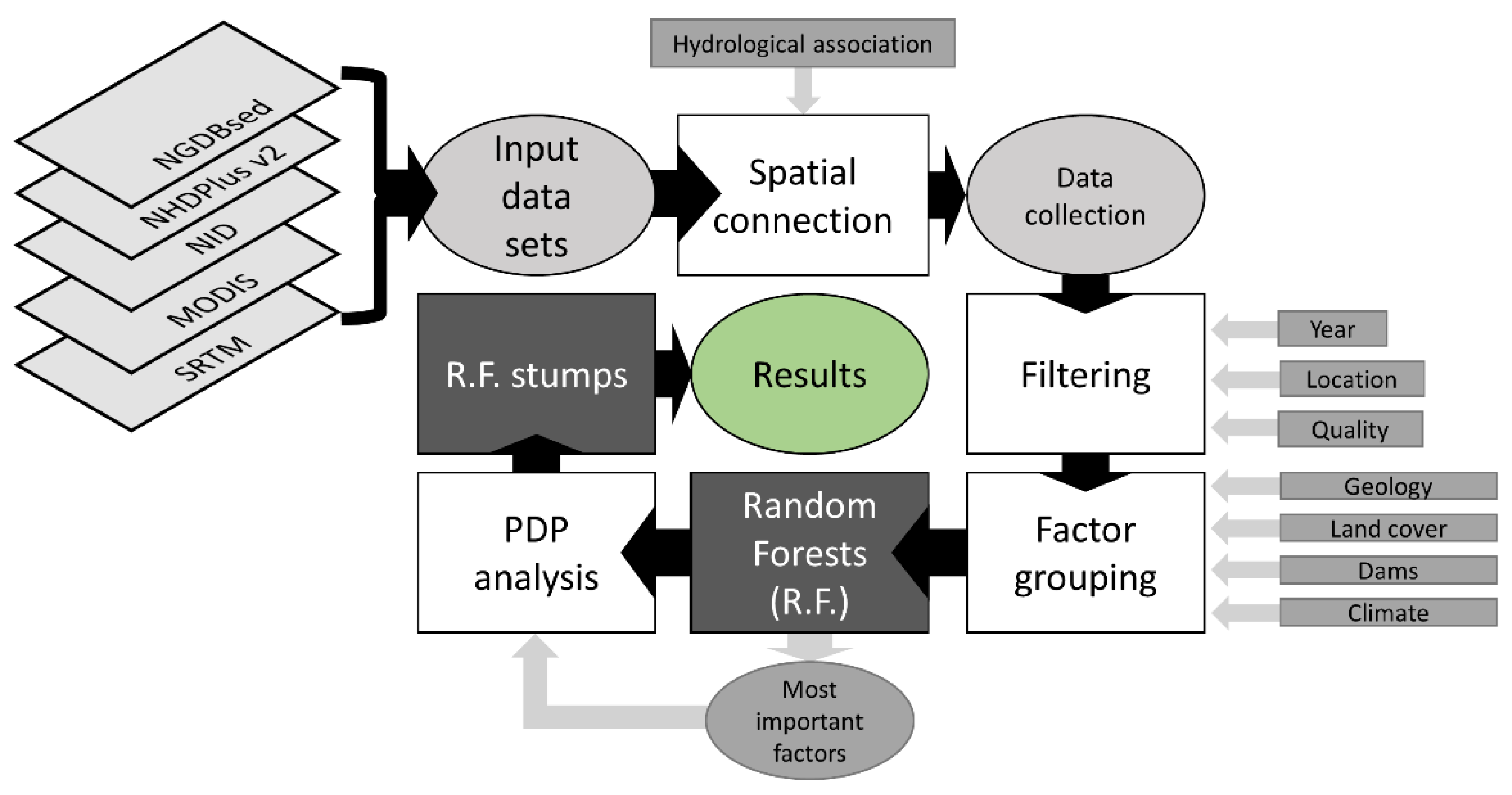
The geochemical sediment data were obtained from the National Geochemical Database (NGDB) sediment database [24], which contains samples taken over the last decades in the United States (Figure 1). The fields in this database describe the sample location, analysis methods, and chemical properties of the sediments. The hydrological information (such as streams, gauging stations, and watershed outlines), as well as many basin attributes, were obtained from the National Hydrological Dataset NHDPlus V2 [25,26]. This dataset allows finding delineated streams and other hydrological features for any point in the U.S. It also contains hundreds of variables ranging from land cover (e.g., land cover types), geology (physical and chemical properties of rocks), soil (e.g., grain size distributions), climate (meteorological variables), and anthropogenic influences that have been accumulated at different levels. The respective information was collected for the accumulated drainage area above the sample location. The information obtained for the watersheds from the NHDPlus was substituted with information from the National Inventory of Dams (NID) [27], which stores information about more than 90,000 dams in the U.S. In the NID, different types of dam construction are distinguished, among them Gravity (PG), which are created from a single block of concrete or stone masonry; Earth (ER), which are constructed from soil; Rockfilled (ER), which are constructed from rocks and boulders; or Timber crib (TC), constructed from wood [28]. Normalized Difference Vegetation Index (NDVI) and Enhanced Vegetation Index (EVI) were obtained from MODIS data. Both indices are based on the infrared reflectance of vegetation measured by satellites. This reflectance varies with vegetation cover and vegetation health [29]. Terrain information such as slope and elevation were extracted from Shuttle Radar Topography Mission (SRTM) data [30,31,32,33].
2.2. Data Collection, Connection, Filtering, and Pre-Processing
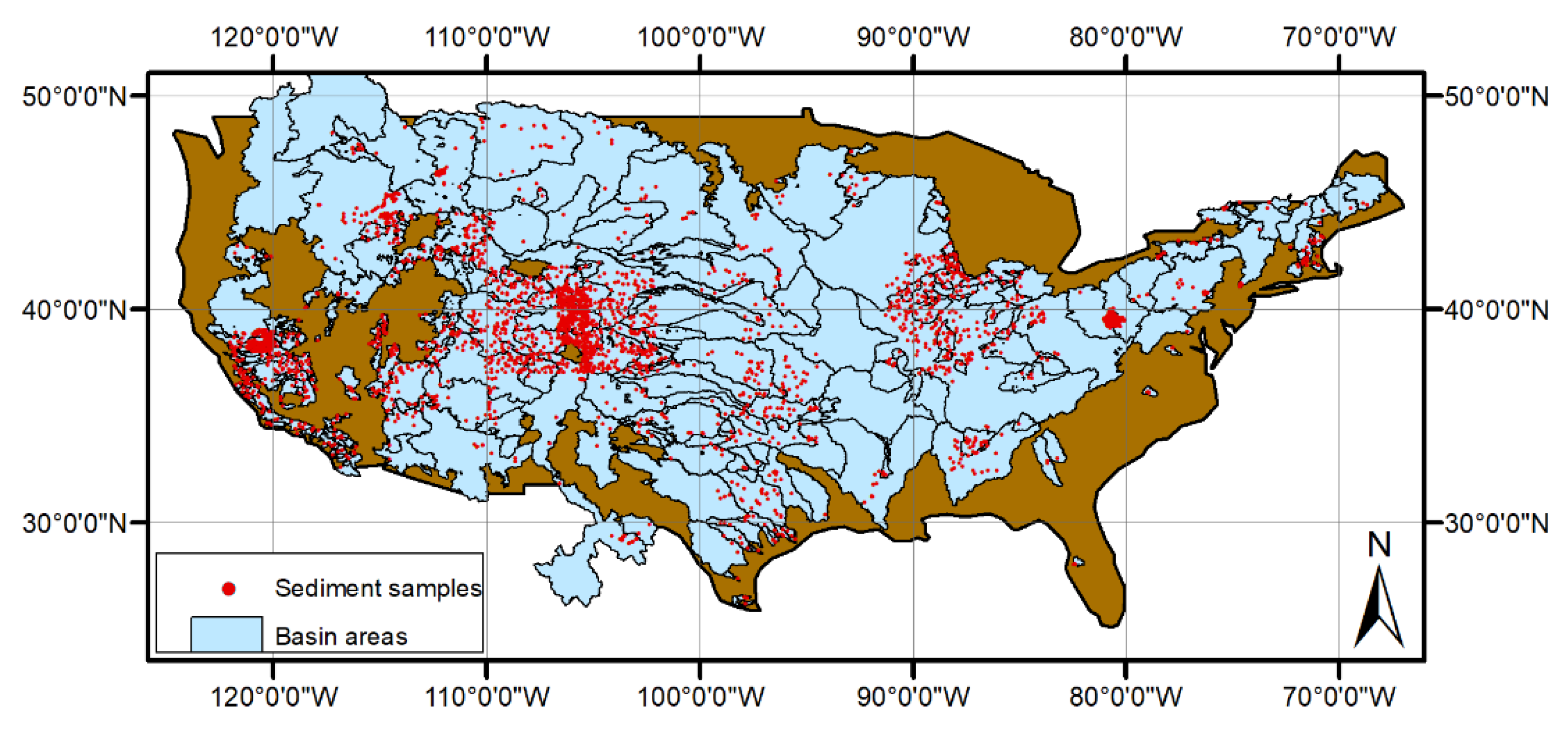
After the data collection, the data were filtered. Only data with a collection date after the year 2000 positioned in the contiguous United States (Figure 2) were included. The cut-off date was selected to ensure that the periods of the different selected datasets would coincide. In addition, only samples that were collected from streams were included. This resulted in differing numbers of samples per metal. The highest number of samples was obtained for Al, with 2927 data entries.
Utilizing the PyGeoHydro library in Python, the closest upstream stream station for each sediment sample was selected from the NHDPlus, and selected attributes for the associated basin above the station were extracted. The minimum, maximum, mean, and median statistics for the NDVI and EVI data and the SRTM digital elevation data were extracted and stored for the same basin. The number of dams of different construction types and attributes, such as length and height of the dam and area and volume of the reservoir, were accumulated per dam type for each basin. The whole data acquisition process resulted in 1684 attributes per sediment sample dataset, describing unique combinations of geology, land cover, soil, climate, and human impact. The Al samples, for example, were associated with 2692 different drainage areas of different sizes and different physical setups. The subsequent statistical analysis was performed in the statistical programming language R (version 4.0.5, R Core Team, Vienna, Austria) in the RStudio environment (version 1.4.1106, RStudio, Boston, MA, USA).
2.3. Factor Grouping
The basin-scale variables were classified into 12 different groups (factor groups, F.G.) based on their associated processes or properties (Table 1). The majority of variables belonged to the group Dams with 1548, while 54 variables were classified into Geology and 32 into Land Cover. The rest of the variables were divided into ten other groups. Supplementary Table S1 lists all variables utilized in the study with a description and their data sources.
The metal concentration data were pre-processed by removing outliers and all values with quality issues. To allow investigation of the metal pollution potential, the data were classified into two groups based on the respective continental average value, representing potential metal concentrations. Values below the mean were classified as “Lower” (L.V.), values equal to or above the mean value were classified as “Higher” (H.V.). Therefore, L.V. can be interpreted as a lower concentration (a lower pollution potential under the given factors), H.V. as a higher potential for metal pollution.
2.4. Random Forest
An approach based on the Random Forest (R.F.) machine learning algorithm was designed for the analysis of the importance of different factors in the determination of the metal pollution potential of river sediments. R.F. has been widely used, including in studies dealing with heavy metal pollution [34,35] and water quality [36,37]. R.F. is an ensemble algorithm that combines decision trees. Through this ensemble, R.F. can learn the patterns in massive datasets and detect non-linear relationships between variables. If the target variable is a categorical variable (classification model), then the majority vote of all trees in the model will be accepted [38]. In the present study, R.F. was trained as a classification model to classify sample sites into L.V. or H.V. In R.F., each tree is grown from a randomly sampled subset of the predictor variables in a process called “bagging”, the selected variables are “in the bag”. The trees do not encounter all the data during model fitting. The remaining data (i.e., out-of-bag, OOB) are used for the OOB validation. The metric of this validation is the OOB error. In a classification model, this error describes the ratio of wrong classifications once the model is confronted with the OOB data, i.e., the previously unseen data [39]. This makes the algorithm inherently robust against overfitting. A manual split of the dataset into a training and a testing dataset is unnecessary for many applications.
A respective R.F. model was trained on all the available data for each metal, resulting in 12 models. There were different numbers of samples available per metal, ranging from 877 to 2927 values. The parameters for each model were set to contain 500 trees per model. After creating each model, the 20 most important variables (MIV) from each of the 12 models were extracted based on the variable importance metric. Variable importance in R.F. denotes the effect of improving prediction at each split and is summarized over all trees in the R.F. model.
2.5. PDP Analysis
Based on the total number of MIV per F.G., a grouping was performed with a Kmeans algorithm. This algorithm initially forms random groups from all cases. Then, it calculates the distance of each group member from the mean of the group. Groups are adjusted until all cases are part of a group so that the summed distance of all cases to their respective group center is minimized. The grouping resulted in four groups. To interpret the relationship between the metal concentration and the explaining factors, partial dependence plots (PDP) for each group were created in R with the pdp package [40]. PDP plots show the likelihood that a selected class is chosen for the dependent in relation to the independent variable.
2.6. R.F. Stumps
In a final analysis of the effects of the MIV on the metals, greatly reduced R.F. models were created containing a single tree with a single decision split. This kind of decision tree is sometimes called a stump due to its minimalistic setup. Five hundred models (for group C3 5000 because of the large number of variables in Dams) were created, and the split variable, threshold, and prediction were recorded. Despite their extreme simplicity, these models achieved OOB errors fluctuating around 32%, i.e., they correctly classified around 68% of the cases. The median value for each variable was combined with the variable importance from the initial larger model.
3. Results
3.1. Individual R.F. Model Performance
To obtain an overview over the performance of the R.F. models in predicting the metal pollution potential, the OOB error can be accessed. Table 2 shows all metals included in the analysis, the number of cases, and the respective OOB error of the fitted R.F. model. There were apparent differences in the OOB error for the different metals. In this classification model (L.V. or H.V.), the OOB error is the rate of wrong classifications. Hence, in Al, 16.5% of cases were allocated to the wrong group (and 83.5% of cases were classified correctly); in Hg, 28.1% were wrongly allocated (and 71.9% were correctly allocated). The overall performance of the individual models was satisfactory, with distinct differences between metals.
3.2. Grouping of the Most Important Factors
To quantify and rank the importance of each F.G. in the determination of the metal pollution potential for all individual metals, the results of the R.F. models were extracted and processed. Table 3 shows the distribution of the 20 MIV of all 12 models into the 12 F.G. The most important F.G. (importance based on the number of associated MIV) was Geology, to which 33 of the MIV belonged, followed by Dams and Land Cover, both with 31 MIV. After this followed Runoff (25 MIV) and Position and Soil (22 MIV each). The least important F.G.s were Population and Channel, with only four and two attributions among the MIV. This shows that there were clear differences in the importance of the F.G. and that the importance of the F.G. depended on the respective metal. A pattern is visible in which some metals share the most important F.G., for example, in Cr and Hg, which both have the highest numbers of MIV in Runoff (four and four) and Climate (five and four). A detailed list of all 240 MIV is presented in supplementary Table S2.
3.3. Meta Groups of Factors
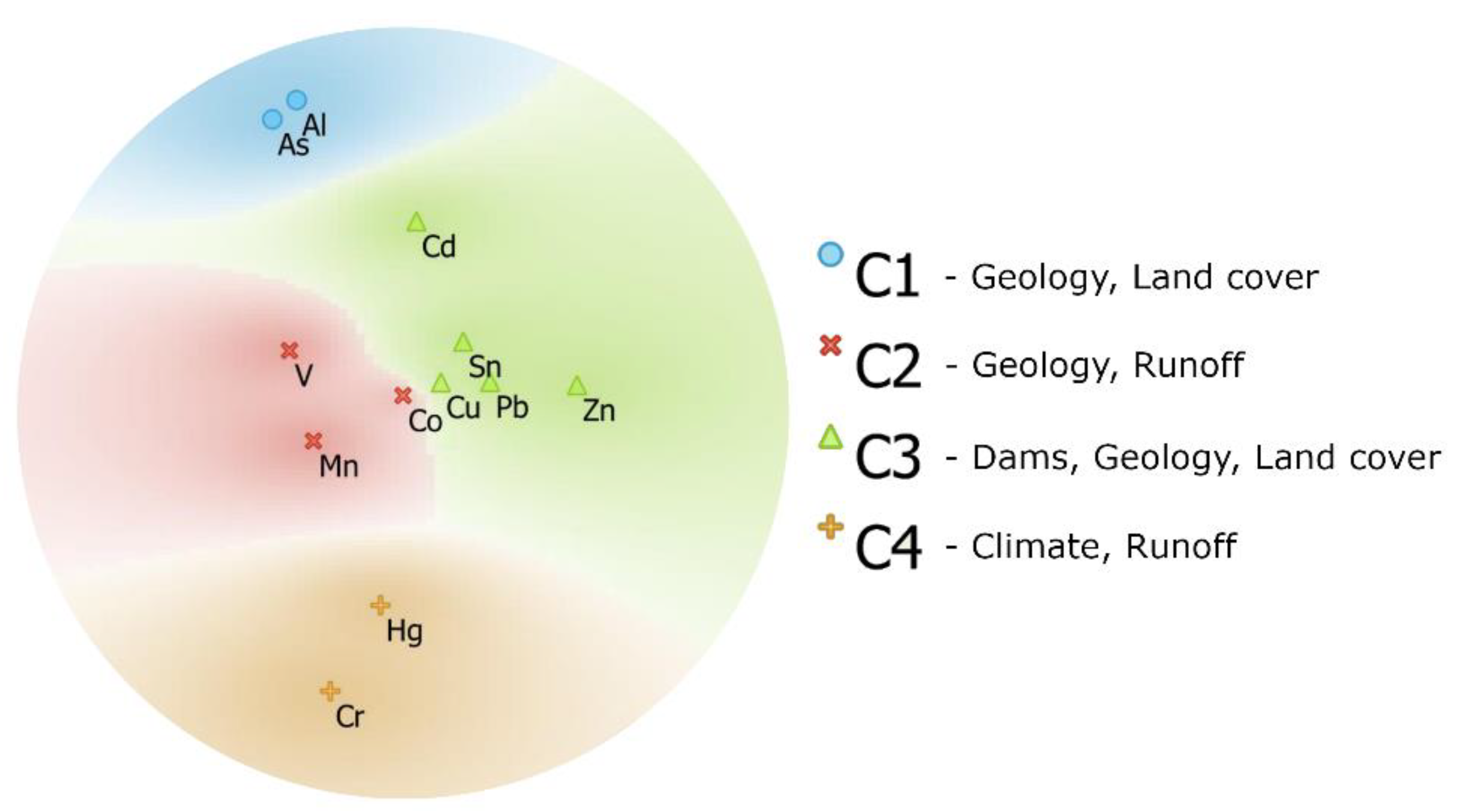
Another way of understanding the importance, especially the interaction of different F.G., is to plot the variables along multiple axes to judge their distributions. This kind of distribution may also allow a grouping. Figure 3 shows a multidimensional projection of the metals in relation to the amount of MIV per F.G. Instead of a two-dimensional coordinate system (x, y), this figure has a six-dimensional coordinate system. The six dimensions are the respective F.G. Land Cover, Geology, Dams, Climate, Runoff, and Position. This selection of F.G. was determined experimentally, and it resulted in the projection in which the silhouettes of the groups were smoothest. The background coloring is based on the Kmeans grouping into the four meta groups, Cluster 1 to Cluster 4 (C1–C4). The grouping indicated the effect of each F.G. on the classification of the respective metal. The affected metals of C1, Al, and As had relatively similar importance of Land Cover and Geology. Group C2, which affected Co, Mn, and V, was defined by the importance of the F.G. Geology and Runoff. The largest group was C3 affecting Cd, Co, Cu, Pb, Sn, and Zn. These metals were grouped by the effect of the F.G. Dams, Land Cover, and Geology. Group C4, which affected Cr and Hg, was mainly defined by Runoff and Climate. These results highlight that some metals have similar dependencies on F.G. and complexes of F.G., making it possible to group them based on their main factors.
3.4. Partial Dependence Plots
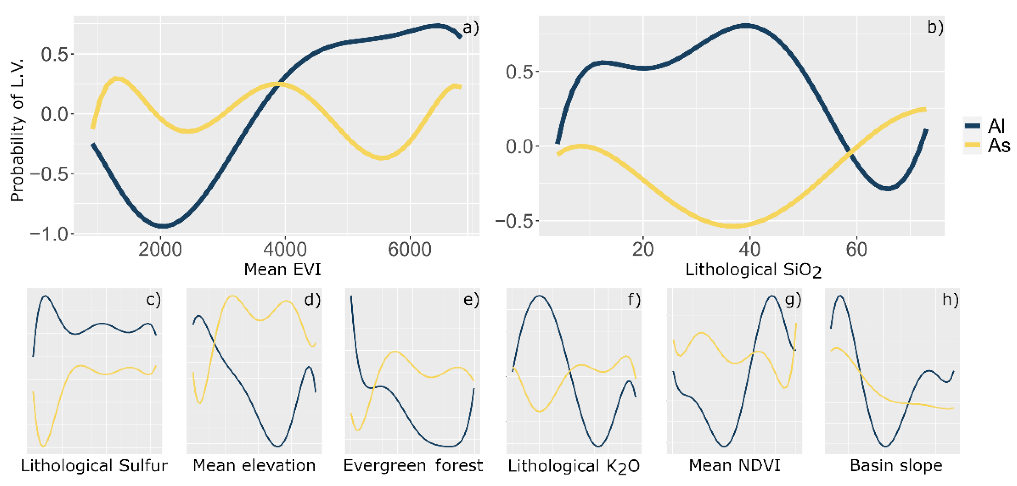
The previous results helped understand the importance of the categorical F.G. in the determination of the metal pollution potential. To understand the effect of individual MIV belonging to the respective F.G., partial dependence plots (PDP) are an effective way to visualize the relationship between dependent and independent variables in a model. Figure 4 shows the partial dependence plots for the variables of the meta group C1. Even though they are in the same group, the two metals have differing, often even opposing, relationships with the same MIV. The mean EVI of the drainage area above the sample location strongly affects Al in (a). In values higher than 2000, there is an increasing probability of classification as L.V. This shows a potential relationship between the size and health of the vegetation cover and Al mobilization and transport processes. The metal As shows some changes along the x-axis but no clear trend. The graph shows contrary relationships for both metals for lithological SiO2 in (b), the basin’s geology’s estimated accumulated lithological SiO2 content. From 0% to 40%, Al increases while As decreases; from then on to higher SiO2 values As increases while Al decreases until 70%. Similar opposing behavior can be seen in plots (d), (e), and especially in (c), which shows a perfect opposite reaction to changes in the sulfur content in the surface rocks of the basin.
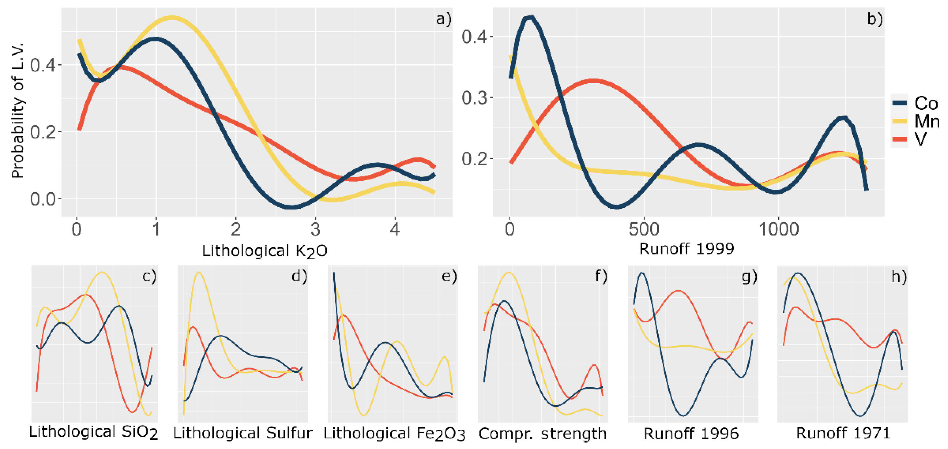
In Figure 5, the PDP for the meta-group C2 is presented. There is a general similarity between the trends of the different lines in many of the plots. In (a), the mean accumulated percentage of lithological K2O content of the rocks in the basin shows a decreasing probability of L.V. for all three metals. The annual runoff in 1999 in (b) shows some deviations, but in general, the trend for the whole group is negative with increasing runoff. The plots (d) and (f) show similar behavior of the curves, while in e) the linear trend of the curves is the same. In (e) and (g), Co and V show an opposing behavior.
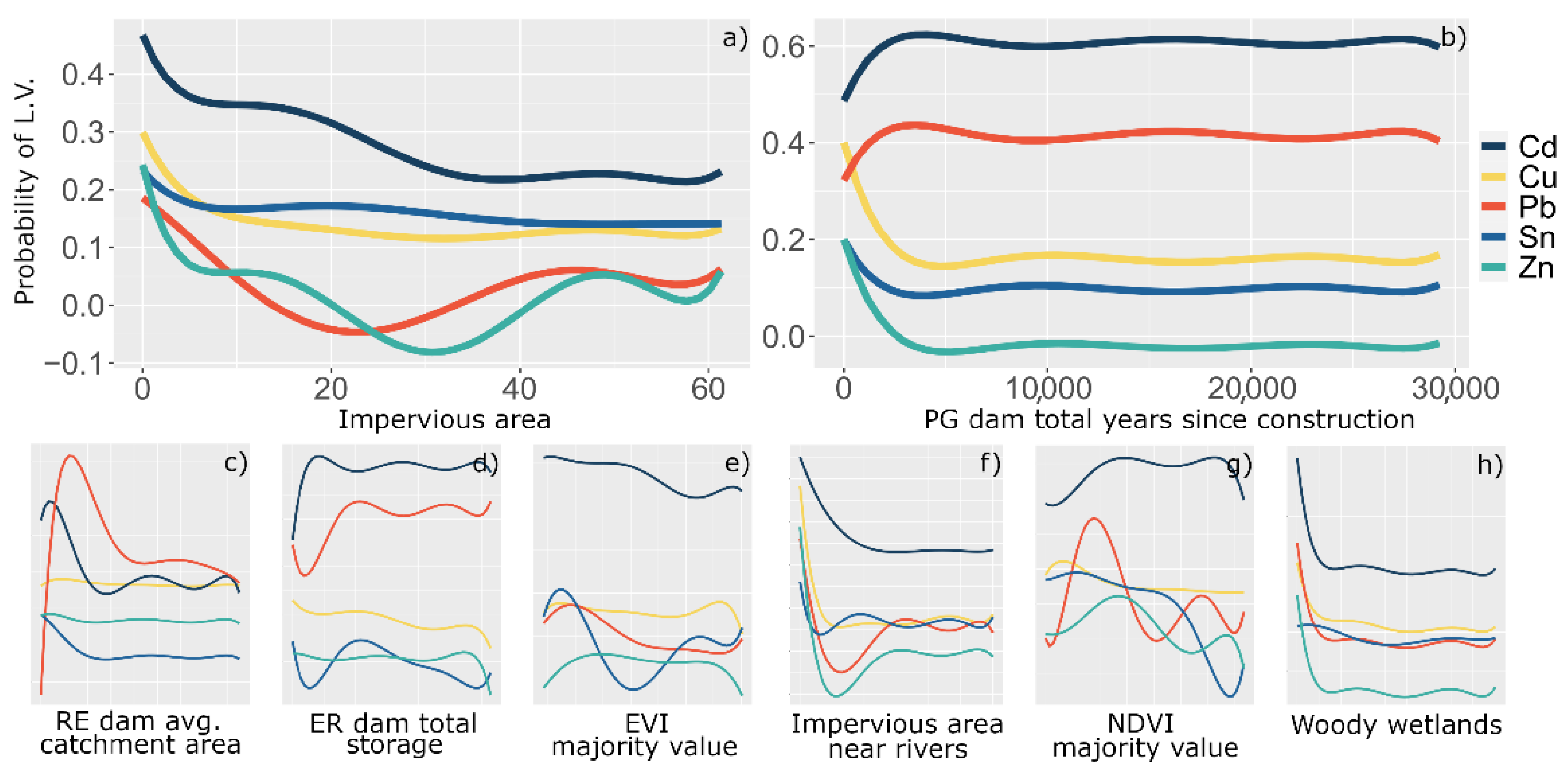
The plots for C3 in Figure 6 show both similarities and differences between the effects of the MIV on the metals in this group. In plot (a), the relationship with the percentage of surface imperviousness in the basin in the year 2001 is similar for Cd, Cu, Pb, Sn, and Zn. The probability of a L.V. generally decreases with an increasing imperviousness. A higher percentage of impervious surfaces indicates a larger presence of human-built structures, such as roads and cities. Pb and Zn show a curve where medium imperviousness values are associated with the lowest probability. It increases in the higher imperviousness range. In plot (b), which shows the relationship with the sum of years since the construction of all dams in the basin that are of the construction type Gravity, it is visible that L.V. of Cd and Pb has a positive relationship with this parameter up until 4000 after which there is little change. At the same time, Cu, Sn, and Zn decrease with increasing values up until 4000, after which they show little change as well. This difference between the effects on the metals is also visible in plot (d), which shows the total storage of all dams of type Rockfill in the basin. Here again, Cd and Pb behave differently from the other three metals. The differing effects of the reservoirs may indicate the dissimilar importance of reservoir effects on these metals. In (f) and (h), all five metals behave similarly with a decreasing linear trend of the probability with increasing impervious surface near rivers and woody wetlands cover, respectively.
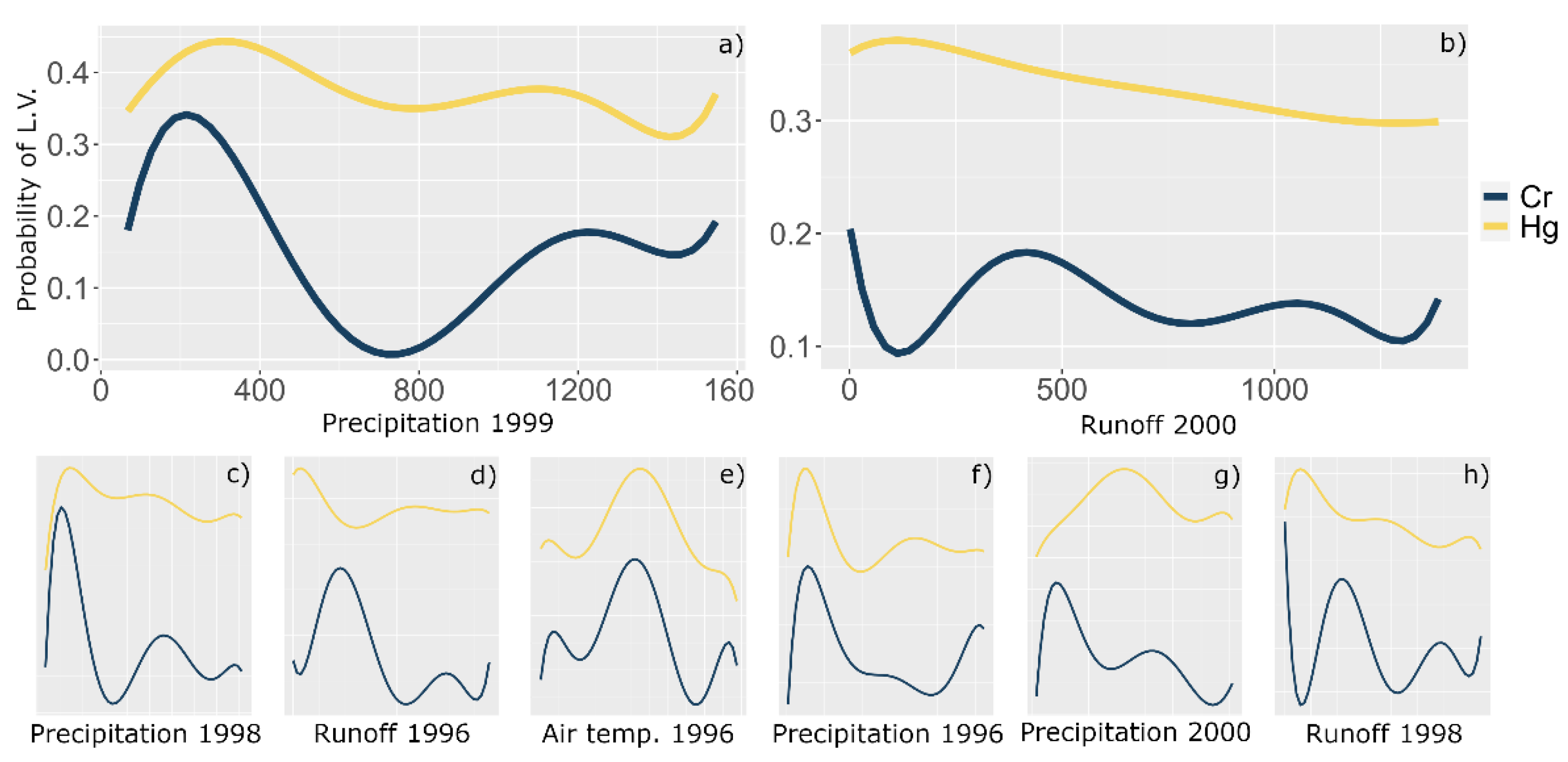
Figure 7 displays the PDP for group C4 consisting of Runoff and Climate and their effects on Cr and Hg. Plot (a) shows the relationship between the probability of L.V. and the annual precipitation in 1999 in the basins. While the specific shape of the curves is different from each other, the general trend is the same. The probability of L.V. decreases first up to 800 mm/a precipitation and then increases again. In (b), which shows the annual runoff of 2000, the curve of Cr shows stronger fluctuations, but its linear trend is similar to that of Hg, the probability of L.V. decreases with increasing runoff. The plots (c), (e), and (f) show similar behavior while (d) shows an opposing behavior in many parts, even if the curve of Hg is much smoother. There is also opposing behavior in (g) after the first 25% of values along the x-axis. In these opposing behaviors, one of the metals reduces while the other increases. These results show that precipitation and runoff affect the amount of transported material in the stream systems.
The PDP analysis shows that the metals have individual dependencies on the factors of the different F.G. Even for those metals within the same meta-group consisting of a collection of F.G., the response may be different.
3.5. R.F. Stump Analysis
The PDP offers a way of investigating the behavior of the probabilities along a gradient of the respective MIV. However, they generally do not facilitate the interpretation of critical decision values that affect the classification result of R.F. To find these critical decision values, the stump analysis was performed. The results of this analysis allow evaluating the values at which the entire dataset is split into a lower or a higher probability of metal pollution. Table 4 shows the results of the stump analysis. In meta-groups C1 and C2, the F.G. Geology has an effect via lithological K2O that differs between the metals. In Al and V, a value for K2O ≤ 2.1 results in a classification as L.V., while in Co and Mn, the same value results in a classification as H.V. Lower elevations cause lower As values in C1, and all classifications below the given NDVI and EVI values are H.V. in Al and As in C1 and for EVI in Sn in C3. In C2 runoff plays a role for all three metals. In Co and Mn, the classification below the given threshold is H.V. For V, the classification below the threshold is L.V. Runoff below a certain threshold in C2 and C4 is strongly associated with H.V. for Co, Mn, Cr, and Hg. Lower precipitation and air temperature values in C4 are associated with H.V. for Cr. In C3, dams play a prominent role, especially the variables describing the average basin size of dams, such as RE dam avg. basin area. In Pb, Sn, and Zn most of these variables lead to a L.V. classification below the threshold. Only the average basin area of ERTC dams in Pb results in a H.V. classification below the threshold. Land Cover in C3 shows a pattern in which woody wetlands below a certain threshold produce a H.V. classification for Cd, Sn, and Zn. The relationship between the metal concentrations in the river sediments and the factors is individually different for most metals.
4. Discussion
4.1. The Factor Groups Geology, Dams, and Land Cover Are Most Important
The metal concentrations depended on these F.G. in differing degrees. The most important F.G. was Geology. Geology was found to play an essential role in many other studies [41,42,43,44]. There are several reasons for this: weathering rocks are an important source of different chemicals. They release these chemicals into soils and the hydrological system, providing a site-specific baseline content of metals as well as other elements that react with metals from different sources. Additionally, the abundance of mines as a source of metals can depend on geological factors. Geology also plays a vital role in developing landscape and soils, which influence hydrological pathways, affecting sediment transport and dissolved chemicals. The results of this study highlight the importance of chemical compounds in the surface geology of the basin, such as K2O, CaO, and SiO2, as determining factors of potential metal pollution. The second most important F.G. was Dams. Dams and their associated reservoirs have been found in other studies to affect sediment and sediment chemistry [45,46]. As potential matter and pollution sinks in the course of streams, they can significantly impact their discharge’s water and sediment chemistry. Our results show that the construction type and average size of the reservoirs drainage areas affect potential metal pollution at a basin scale. The dam construction type is often associated with the reservoir size, the terrain, and other local conditions, which may explain the relationship between construction type and effect on metal concentration. Land Cover was the third most important F.G. Land cover is another well-documented factor of soil- and hydrochemistry [47,48,49]. Different land cover types are associated with different intensities of human impact and different hydrological processes. Especially agricultural land cover can be a source of many chemical compounds due to metal-containing agricultural chemicals and irrigation practices [50,51]. Our results show that vegetation indices (NDVI and EVI) seem to be better indicators of metal pollution potential than percentages of individual land cover types. One reason for this may be that NDVI and EVI implicitly include information about vegetation health status and canopy coverage [52,53]. These attributes of vegetation affect rock weathering, soil erosion, and especially transport processes in surface runoff [54,55,56].
4.2. Rock Chemistry, Vegetation Indices, and Precipitation Affect Metal Concentrations
We found that in Geology, lithological K2O, CaO, and SiO2 were the most important factors based on their importance in the R.F. models (Table 4). The rocks with these contents possibly provide chemicals during weathering that affect the mobility of some of the metals. SiO2 is a component of clay minerals, which have been demonstrated to actively reduce heavy metals in water and soil [57,58]. The same has been observed for CaO, which may promote the formation of soil aggregates binding heavy metals [59]. In our results, K2O reduces Co and Mn, which agrees with the findings in other studies [60]. However, for Al and V, higher values of K2O increase metal content (K2O ≤ 2.1 = L.V.). The mechanisms behind this result require further investigation. Our results show that for Dams, the essential variables were those dealing with Dams’ average size and discharge. Reservoirs play a vital role in the sediment movement in rivers [46,61,62], and larger reservoirs may have a more substantial effect on the transport processes than smaller ones. Many studies have found a connection between vegetation indices such as NDVI and EVI and catchment sediment discharge [63,64]. We found that the importance of NDVI and EVI was generally higher than that of specific land cover types. They are closely connected to the type and health of the vegetation in a catchment, which is closely related to soil erosion processes [65,66,67]. For Runoff, the runoff in 1996 seemed to play an important role. It appears that 1996 was a year in which periods of nationwide drought and periods of nationwide overly wet conditions occurred [68], which may have affected matter transport and vegetation health. In the F.G. Climate precipitation and air temperature played a role, especially in the year 1996. The importance of Position can probably be explained by the effect of the geogenic background emission of metals from weathering rocks and local climate.
4.3. Factor Meta Groups Affect Metals Differently
Interestingly, there were apparent differences in the importance of each F.G. for the respective metals. The differing numbers of MIV per F.G. allowed grouping the metals based on the respective importance of each F.G. (Table 3). This kind of clustering or grouping of chemical concentrations based on source factors has been performed successfully elsewhere [69,70]. The results were four meta groups of basin-scale factors (Figure 3). In C1, Geology, Land Cover, and Terrain are components of the landscape that intensely influence each other and affect hydrological processes at many levels [71,72,73]. This group had a strong effect on Al and As, but we found the opposite effect for the two metals in many cases. In C2, Geology affects runoff processes at many scales by forming geomorphological features and the effect on groundwater movements [71,74]. Furthermore, the geology of a site determines the kind of rock available for weathering, which releases different elements into soil and water [75]. Co, Mn, and V were affected strongest by this group. The effect was often the same for all three metals, i.e., the (linear) trends of their changes were similar in the plots (a), (b), (d), and (f) (Figure 5). In C3, we found that Land Cover showed a strong effect together with the F.G. Dams. Dammed reservoirs play an important role as sources and sinks in the hydrological system [76] and may modulate the effects of land cover on soil and water chemistry and transport mechanisms. Affected by C3 were Cd, Cu, Pb, Sn, and Zn (Figure 3). Often, Cd and Pb behaved differently from the metals in this group. In C4, Runoff is fundamentally driven by the climate through precipitation. The landscape with geology, soils, and vegetation mostly modulates the discharge response to climate events [77,78,79]. Both affected metals, Cr and Hg, were affected similarly by changes in the MIV associated with this group.
4.4. Basin-Scale Factors Hold Enough Information to Predict Potential Metal Pollution
Differing degrees of accuracy for different chemical elements are common and have been observed elsewhere when using R.F. or other models [35,80]. Several reasons for differing performance come to mind: (1) Differences in the quality of the measured concentration data. There could be an observation bias, i.e., those specific elements have been measured under certain conditions that may not represent the general distribution of such elements. (2) Differences in required input data. It may be that necessary input variables and data, which play an important role in the processes that lead to the chemical concentrations, are not present in the selection of variables created for this study. In addition, spatial effects could play a role in the determination of metal concentrations. The concentration of Hg, for example, could be stronger affected by processes and sources in the direct proximity of the sampling site rather than by factors at the basin scale. (3) Differences in origin and transport and accumulation processes. These differ based on many combinations of physical factors [81,82,83]. These may interact with the chemical properties and behavior of the studied elements to form complex patterns [84,85,86] that could not be captured with the present data or methods.
The R.F. models were set up with data accumulated at the basin scale. They generally performed well in categorizing the sediment concentrations of the twelve metals. The best performance was found for Al, with an OOB error of 16.5%. The poorest performance was found for Hg, with an OOB error of 28.1% (Table 2). Our results indicate that the information accumulated to the basin level can be utilized to predict a potential metal concentration for most metals. Moreover, this study’s finding is that the results differ greatly between the metals, even though the same input data were available for all samples. This indicates differences in the power of the basin-scale to predict metal concentrations. These differences may not have been detected in a study focused on fewer metals.
4.5. Limitations and Considerations
Several limitations can be observed in the presented methods: (1) The input data are a limiting factor, and more data should theoretically make the models more robust. R.F. can handle large datasets just as easily as smaller datasets. However, some potentially important data were not available in the utilized datasets. For example, there were no hydro-chemical parameters stored in the database. Parameters such as stream pH, oxygen content, hardness, or alkalinity were not available to the same degree as the other data. Another type of data not included was the extent of levee construction in the respective areas. The effects of levees on the connectivity between floodplain and river may play an important role in a part of the studied areas. In these areas, the absence of data describing lateral connectivity might lead to miscalculations of the importance of factors. However, most of the studied sites in this research were in areas of the US with few or no levees. (2) There is a bias of the methodology towards F.G. with more variables, which results in a focus on the bigger factor groups such as Dams, Geology, and Land Cover. This affects the grouping of the metals into the meta groups. Still, the variables from all F.G. contributed to the final estimation of metal pollution potential. (3) Several R.F. models created from the same data will show slightly different results. That is why a relatively large number of MIV was selected, because the most important variable in one model may be the second- or fourth-most important variable in the next model created from the same data.
Furthermore, several issues should be considered: (1) The features included in the study are spatially not homogeneous. The number of dams in the NID database is much higher in the eastern parts of the USA [87], and patterns are visible in which dams are associated with a more pronounced terrain. Climate is spatially heterogeneous, showing large-scale differences between wetter and dryer regions of the country. There are differences in the established vegetation and associated vegetation indices in connection with these climate patterns. Finally, the distribution of the sediment samples (Figure 2) shows that these are not evenly scattered over the country. The effects of the spatial coincidence of different attributes and the consequences for determining basin-scale factors affecting metal pollution would pose an interesting research question. (2) The scope of this research was the basin-scale factors of metal concentrations in sediments. This means that often important point sources of metals and other chemicals were not represented in the datasets. Among these point-sources are ports and other water transport facilities and metallurgical and industrial enterprises. The spatially heterogeneous distribution of these sources makes it challenging to represent them adequately at the basin scale. (3) As shown in Supplementary Table S3, the majority of drainage areas in the study dataset was smaller than 1000 km2. Therefore, the validity of our results for drainage areas larger than 1000 km2 may be limited.
5. Conclusions
This study found that many factors at the basin scale affect metal concentrations and, thus, metal pollution potential in river sediment to varying degrees. The most important were Geology, Dams, and Land Cover. These formed meta groups with other variable types associated with effects on the concentration of specific metals in the sediment. Most of the presented R.F. models performed quite well in predicting potential metal concentrations. Thus, many of the concentrations seem to be partly to largely determined by basin-scale factors. Random Forest as a machine learning algorithm proved capable of finding these relationships. The presented results can be used as a basis for further study of specific relationships, for selecting input data for machine learning or other approaches to heavy metal studies, or as a basis for studies about mitigation strategies involving land cover change management.
Supplementary Materials
The following supporting information can be downloaded at: https://0-www-mdpi-com.brum.beds.ac.uk/article/10.3390/app12062805/s1, Table S1: Detailed list of used variables and data sources; Table S2: Detailed list of all 240 MIV; Table S3: The list of the studied drainage areas.
Author Contributions
Conceptualization, T.L.; methodology, T.L.; software, T.L.; validation, T.L.; formal analysis, T.L. and C.O.; investigation, T.L.; resources, T.L. and C.O.; data curation, T.L.; writing—original draft preparation, T.L.; writing—review and editing, T.L. and C.O.; visualization, T.L.; supervision, T.L.; project administration, T.L.; funding acquisition, T.L. All authors have read and agreed to the published version of the manuscript.
Funding
This research was funded by the scientific research start-up fund for high-level talents of Jinling Institute of Technology: jit-b-202139.
Institutional Review Board Statement
Not applicable.
Informed Consent Statement
Not applicable.
Data Availability Statement
The authors confirm that the data supporting the findings of this study are available within the article and its Supplementary Materials.
Conflicts of Interest
The authors declare no conflict of interest.
References
- Matys Grygar, T.; Elznicová, J.; Kiss, T.; Smith, H.G. Using sedimentary archives to reconstruct pollution history and sediment provenance: The Ohře River, Czech Republic. Catena 2016, 144, 109–129. [Google Scholar] [CrossRef]
- Marziali, L.; Valsecchi, L.; Schiavon, A.; Mastroianni, D.; Viganò, L. Vertical profiles of trace elements in a sediment core from the Lambro River (northern Italy): Historical trends and pollutant transport to the Adriatic Sea. Sci. Total Environ. 2021, 782, 146766. [Google Scholar] [CrossRef] [PubMed]
- Park, E.; Lim, J.; Ho, H.L.; Herrin, J.; Chitwatkulsiri, D. Source-to-sink sediment fluxes and budget in the Chao Phraya River, Thailand: A multi-scale analysis based on the national dataset. J. Hydrol. 2021, 594, 125643. [Google Scholar] [CrossRef]
- Zhang, D.; Xie, W.; Shen, J.; Guo, L.; Chen, Y.; He, Q. Sediment dynamics in the mudbank of the Yangtze River Estuary under regime shift of source and sink. Int. J. Sediment Res. 2022, 37, 97–109. [Google Scholar] [CrossRef]
- Zhou, Q.; Yang, N.; Li, Y.; Ren, B.; Ding, X.; Bian, H.; Yao, X. Total concentrations and sources of heavy metal pollution in global river and lake water bodies from 1972 to 2017. Glob. Ecol. Conserv. 2020, 22, e00925. [Google Scholar] [CrossRef]
- Kumar, V.; Parihar, R.D.; Sharma, A.; Bakshi, P.; Singh Sidhu, G.P.; Bali, A.S.; Karaouzas, I.; Bhardwaj, R.; Thukral, A.K.; Gyasi-Agyei, Y.; et al. Global evaluation of heavy metal content in surface water bodies: A meta-analysis using heavy metal pollution indices and multivariate statistical analyses. Chemosphere 2019, 236, 124364. [Google Scholar] [CrossRef]
- Olawoyin, R.; Oyewole, S.A.; Grayson, R.L. Potential risk effect from elevated levels of soil heavy metals on human health in the Niger delta. Ecotoxicol. Environ. Saf. 2012, 85, 120–130. [Google Scholar] [CrossRef]
- Cai, L.-M.; Xu, Z.-C.; Qi, J.-Y.; Feng, Z.-Z.; Xiang, T.-S. Assessment of exposure to heavy metals and health risks among residents near Tonglushan mine in Hubei, China. Chemosphere 2015, 127, 127–135. [Google Scholar] [CrossRef]
- Swarnkumar, R.; Osborne, W.J. Heavy metal determination and aquatic toxicity evaluation of textile dyes and effluents using Artemia salina. Biocatal. Agric. Biotechnol. 2020, 25, 101574. [Google Scholar] [CrossRef]
- Uddin, M.J.; Jeong, Y.-K. Urban river pollution in Bangladesh during last 40 years: Potential public health and ecological risk, present policy, and future prospects toward smart water management. Heliyon 2021, 7, e06107. [Google Scholar] [CrossRef]
- Liu, Z.; Fei, Y.; Shi, H.; Mo, L.; Qi, J. Prediction of high-risk areas of soil heavy metal pollution with multiple factors on a large scale in industrial agglomeration areas. Sci. Total Environ. 2022, 808, 151874. [Google Scholar] [CrossRef] [PubMed]
- Mora, A.; Jumbo-Flores, D.; González-Merizalde, M.; Bermeo-Flores, S.A.; Alvarez-Figueroa, P.; Mahlknecht, J.; Hernández-Antonio, A. Heavy Metal Enrichment Factors in Fluvial Sediments of an Amazonian Basin Impacted by Gold Mining. Bull. Environ. Contam. Toxicol. 2019, 102, 210–217. [Google Scholar] [CrossRef] [PubMed]
- Yang, H.J.; Bong, K.M.; Kang, T.-W.; Hwang, S.H.; Na, E.H. Assessing heavy metals in surface sediments of the Seomjin River Basin, South Korea, by statistical and geochemical analysis. Chemosphere 2021, 284, 131400. [Google Scholar] [CrossRef] [PubMed]
- Li, M.; Zhang, Q.; Sun, X.; Karki, K.; Zeng, C.; Pandey, A.; Rawat, B.; Zhang, F. Heavy metals in surface sediments in the trans-Himalayan Koshi River catchment: Distribution, source identification and pollution assessment. Chemosphere 2020, 244, 125410. [Google Scholar] [CrossRef] [PubMed]
- Paul, V.; Sankar, M.S.; Vattikuti, S.; Dash, P.; Arslan, Z. Pollution assessment and land use land cover influence on trace metal distribution in sediments from five aquatic systems in southern USA. Chemosphere 2021, 263, 128243. [Google Scholar] [CrossRef] [PubMed]
- Allafta, H.; Opp, C. Spatio-temporal variability and pollution sources identification of the surface sediments of Shatt Al-Arab River, Southern Iraq. Sci. Rep. 2020, 10, 6979. [Google Scholar] [CrossRef]
- Yin, H.; Islam, M.S.; Ju, M. Urban river pollution in the densely populated city of Dhaka, Bangladesh: Big picture and rehabilitation experience from other developing countries. J. Clean. Prod. 2021, 321, 129040. [Google Scholar] [CrossRef]
- El-Anwar, E.A.; Salman, S.; Asmoay, A.; Elnazer, A. Geochemical, mineralogical and pollution assessment of River Nile sediments at Assiut Governorate, Egypt. J. Afr. Earth Sci. 2021, 180, 104227. [Google Scholar] [CrossRef]
- Qin, G.; Niu, Z.; Yu, J.; Li, Z.; Ma, J.; Xiang, P. Soil heavy metal pollution and food safety in China: Effects, sources and removing technology. Chemosphere 2021, 267, 129205. [Google Scholar] [CrossRef]
- Ding, J.; Jiang, Y.; Liu, Q.; Hou, Z.; Liao, J.; Fu, L.; Peng, Q. Influences of the land use pattern on water quality in low-order streams of the Dongjiang River basin, China: A multi-scale analysis. Sci. Total Environ. 2016, 551–552, 205–216. [Google Scholar] [CrossRef]
- Bostanmaneshrad, F.; Partani, S.; Noori, R.; Nachtnebel, H.-P.; Berndtsson, R.; Adamowski, J.F. Relationship between water quality and macro-scale parameters (land use, erosion, geology, and population density) in the Siminehrood River Basin. Sci. Total Environ. 2018, 639, 1588–1600. [Google Scholar] [CrossRef] [PubMed]
- Xu, S.; Li, S.-L.; Zhong, J.; Li, C. Spatial scale effects of the variable relationships between landscape pattern and water quality: Example from an agricultural karst river basin, Southwestern China. Agric. Ecosyst. Environ. 2020, 300, 106999. [Google Scholar] [CrossRef]
- Huang, S.; Xiao, L.; Zhang, Y.; Wang, L.; Tang, L. Interactive effects of natural and anthropogenic factors on heterogenetic accumulations of heavy metals in surface soils through geodetector analysis. Sci. Total Environ. 2021, 789, 147937. [Google Scholar] [CrossRef]
- USGS. National Geochemical Database: Sediment; U.S. Geological Survey: Reston, VA, USA, 2016.
- Moore, R.B.; Dewald, T.G. The Road to NHDPlus—Advancements in Digital Stream Networks and Associated Catchments. JAWRA J. Am. Water Resour. Assoc. 2016, 52, 890–900. [Google Scholar] [CrossRef] [Green Version]
- McKay, L.; Bondelit, T.; Dewald, T.; Johnston, J.; Moore, R.; Rea, A. NHDPlus Version 2: User Guide. Available online: https://nhdplus.com/NHDPlus/NHDPlusV2_documentation.php (accessed on 15 December 2021).
- USACE. National Inventory of Dams (NID); U.S. Army Corps of Engineers (USACE): Washington, DC, USA, 2016.
- Breeze, P. Chapter 3-Dams and Barrages. In Hydropower; Breeze, P., Ed.; Academic Press: Cambridge, MA, USA, 2018; pp. 23–33. [Google Scholar]
- Didan, K. MOD13A1 MODIS/Terra Vegetation Indices 16-Day L3 Global 500 m SIN Grid V006 [Data set]. NASA EOSDIS Land Processes DAAC 2015, 10, 415. [Google Scholar] [CrossRef]
- Farr, T.; Rosen, P.; Caro, E.; Crippen, R.; Duren, R.; Hensley, S.; Kobrick, M.; Paller, M.; Rodriguez, E.; Roth, L.; et al. The Shuttle Radar Topography Mission. Rev. Geophys. 2007, 45, RG2004. [Google Scholar] [CrossRef] [Green Version]
- Farr, T.G.; Kobrick, M. Shuttle radar topography mission produces a wealth of data. Eos Trans. Am. Geophys. Union 2011, 81, 583–585. [Google Scholar] [CrossRef]
- NASA. NASA Shuttle Radar Topography Mission Global 1 arc second [Data set]. NASA EOSDIS Land Processes DAAC 2013. [Google Scholar] [CrossRef]
- Rosen, P.A.; Hensley, S.; Joughin, I.R.; Li, F.K.; Madsen, S.N.; Rodriguez, E.; Goldstein, R.M. Synthetic aperture radar interferometry. Proc. IEEE 2000, 88, 333–382. [Google Scholar] [CrossRef]
- Li, X.; Geng, T.; Shen, W.; Zhang, J.; Zhou, Y. Quantifying the influencing factors and multi-factor interactions affecting cadmium accumulation in limestone-derived agricultural soil using random forest (RF) approach. Ecotoxicol. Environ. Saf. 2021, 209, 111773. [Google Scholar] [CrossRef]
- Tan, K.; Ma, W.; Wu, F.; Du, Q. Random forest-based estimation of heavy metal concentration in agricultural soils with hyperspectral sensor data. Environ. Monit. Assess. 2019, 191, 446. [Google Scholar] [CrossRef]
- Wang, F.; Wang, Y.; Zhang, K.; Hu, M.; Weng, Q.; Zhang, H. Spatial heterogeneity modeling of water quality based on random forest regression and model interpretation. Environ. Res. 2021, 202, 111660. [Google Scholar] [CrossRef] [PubMed]
- Harrison, J.W.; Lucius, M.A.; Farrell, J.L.; Eichler, L.W.; Relyea, R.A. Prediction of stream nitrogen and phosphorus concentrations from high-frequency sensors using Random Forests Regression. Sci. Total Environ. 2021, 763, 143005. [Google Scholar] [CrossRef] [PubMed]
- Fouedjio, F. Classification random forest with exact conditioning for spatial prediction of categorical variables. Artif. Intell. Geosci. 2021, 2, 82–95. [Google Scholar] [CrossRef]
- Breiman, L. Random Forests. Mach. Learn. 2001, 45, 5–32. [Google Scholar] [CrossRef] [Green Version]
- Greenwell, B.M. pdp: An R Package for Constructing Partial Dependence Plots. R J. 2017, 9, 421–436. [Google Scholar] [CrossRef] [Green Version]
- Reczyński, W.; Szarłowicz, K.; Jakubowska, M.; Bitusik, P.; Kubica, B. Comparison of the sediment composition in relation to basic chemical, physical, and geological factors. Int. J. Sediment Res. 2020, 35, 307–314. [Google Scholar] [CrossRef]
- Karimi, A.; Haghnia, G.H.; Ayoubi, S.; Safari, T. Impacts of geology and land use on magnetic susceptibility and selected heavy metals in surface soils of Mashhad plain, northeastern Iran. J. Appl. Geophys. 2017, 138, 127–134. [Google Scholar] [CrossRef]
- Khan, S.; Rehman, S.; Zeb Khan, A.; Amjad Khan, M.; Tahir Shah, M. Soil and vegetables enrichment with heavy metals from geological sources in Gilgit, northern Pakistan. Ecotoxicol. Environ. Saf. 2010, 73, 1820–1827. [Google Scholar] [CrossRef]
- Sanz-Prada, L.; Garcia-Ordiales, E.; Flor-Blanco, G.; Roqueñí, N.; Álvarez, R. Determination of heavy metal baseline levels and threshold values on marine sediments in the Bay of Biscay. J. Environ. Manag. 2022, 303, 114250. [Google Scholar] [CrossRef]
- Zhao, Q.; Ding, S.; Lu, X.; Liang, G.; Hong, Z.; Lu, M.; Jing, Y. Water-sediment regulation scheme of the Xiaolangdi Dam influences redistribution and accumulation of heavy metals in sediments in the middle and lower reaches of the Yellow River. Catena 2022, 210, 105880. [Google Scholar] [CrossRef]
- Reczynski, W.; Jakubowska, M.; Golas, J.; Parker, A.; Kubica, B. Chemistry of sediments from the Dobczyce Reservoir, Poland, and the environmental implications. Int. J. Sediment Res. 2010, 25, 28–38. [Google Scholar] [CrossRef]
- Yang, Y.; Yang, X.; He, M.; Christakos, G. Beyond mere pollution source identification: Determination of land covers emitting soil heavy metals by combining PCA/APCS, GeoDetector and GIS analysis. Catena 2020, 185, 104297. [Google Scholar] [CrossRef]
- Wang, Z.; Xiao, J.; Wang, L.; Liang, T.; Guo, Q.; Guan, Y.; Rinklebe, J. Elucidating the differentiation of soil heavy metals under different land uses with geographically weighted regression and self-organizing map. Environ. Pollut. 2020, 260, 114065. [Google Scholar] [CrossRef] [PubMed]
- Lisiak-Zielińska, M.; Borowiak, K.; Budka, A.; Kanclerz, J.; Janicka, E.; Kaczor, A.; Żyromski, A.; Biniak-Pieróg, M.; Podawca, K.; Mleczek, M.; et al. How polluted are cities in central Europe?—Heavy metal contamination in Taraxacum officinale and soils collected from different land use areas of three representative cities. Chemosphere 2021, 266, 129113. [Google Scholar] [CrossRef] [PubMed]
- Wang, X.; Liu, W.; Li, Z.; Teng, Y.; Christie, P.; Luo, Y. Effects of long-term fertilizer applications on peanut yield and quality and plant and soil heavy metal accumulation. Pedosphere 2020, 30, 555–562. [Google Scholar] [CrossRef]
- ur Rehman, K.; Bukhari, S.M.; Andleeb, S.; Mahmood, A.; Erinle, K.O.; Naeem, M.M.; Imran, Q. Ecological risk assessment of heavy metals in vegetables irrigated with groundwater and wastewater: The particular case of Sahiwal district in Pakistan. Agric. Water Manag. 2019, 226, 105816. [Google Scholar] [CrossRef]
- Bento, V.A.; Gouveia, C.M.; DaCamara, C.C.; Libonati, R.; Trigo, I.F. The roles of NDVI and Land Surface Temperature when using the Vegetation Health Index over dry regions. Glob. Planet. Chang. 2020, 190, 103198. [Google Scholar] [CrossRef]
- Tenreiro, T.R.; García-Vila, M.; Gómez, J.A.; Jiménez-Berni, J.A.; Fereres, E. Using NDVI for the assessment of canopy cover in agricultural crops within modelling research. Comput. Electron. Agric. 2021, 182, 106038. [Google Scholar] [CrossRef]
- Epp, T.; Neidhardt, H.; Pagano, N.; Marks, M.A.W.; Markl, G.; Oelmann, Y. Vegetation canopy effects on total and dissolved Cl, Br, F and I concentrations in soil and their fate along the hydrological flow path. Sci. Total Environ. 2020, 712, 135473. [Google Scholar] [CrossRef]
- Liu, X.; Zhou, Z.; Ding, Y. Vegetation coverage change and erosion types impacts on the water chemistry in western China. Sci. Total Environ. 2021, 772, 145543. [Google Scholar] [CrossRef]
- Zakharova, E.A.; Pokrovsky, O.S.; Dupré, B.; Gaillardet, J.; Efimova, L.E. Chemical weathering of silicate rocks in Karelia region and Kola peninsula, NW Russia: Assessing the effect of rock composition, wetlands and vegetation. Chem. Geol. 2007, 242, 255–277. [Google Scholar] [CrossRef]
- Otunola, B.O.; Ololade, O.O. A review on the application of clay minerals as heavy metal adsorbents for remediation purposes. Environ. Technol. Innov. 2020, 18, 100692. [Google Scholar] [CrossRef]
- Liang, X.; Han, J.; Xu, Y.; Sun, Y.; Wang, L.; Tan, X. In situ field-scale remediation of Cd polluted paddy soil using sepiolite and palygorskite. Geoderma 2014, 235–236, 9–18. [Google Scholar] [CrossRef]
- Mallampati, S.R.; Mitoma, Y.; Okuda, T.; Sakita, S.; Kakeda, M. Enhanced heavy metal immobilization in soil by grinding with addition of nanometallic Ca/CaO dispersion mixture. Chemosphere 2012, 89, 717–723. [Google Scholar] [CrossRef] [PubMed]
- Ribeiro, P.G.; Souza, J.M.P.; Rodrigues, M.; Ribeiro, I.C.A.; de Carvalho, T.S.; Lopes, G.; Li, Y.C.; Guilherme, L.R.G. Hydrothermally-altered feldspar as an environmentally-friendly technology to promote heavy metals immobilization: Batch studies and application in smelting-affected soils. J. Environ. Manag. 2021, 291, 112711. [Google Scholar] [CrossRef]
- Cheng, Y.; Zhao, F.; Wu, J.; Gao, P.; Wang, Y.; Wang, J. Migration characteristics of arsenic in sediments under the influence of cascade reservoirs in Lancang River basin. J. Hydrol. 2022, 606, 127424. [Google Scholar] [CrossRef]
- Sohoulande Djebou, D.C. Assessment of sediment inflow to a reservoir using the SWAT model under undammed conditions: A case study for the Somerville reservoir, Texas, USA. Int. Soil Water Conserv. Res. 2018, 6, 222–229. [Google Scholar] [CrossRef]
- Ye, S.; Ran, Q.; Fu, X.; Hu, C.; Wang, G.; Parker, G.; Chen, X.; Zhang, S. Emergent stationarity in Yellow River sediment transport and the underlying shift of dominance: From streamflow to vegetation. Hydrol. Earth Syst. Sci. 2019, 23, 549–556. [Google Scholar] [CrossRef] [Green Version]
- Ouyang, W.; Hao, F.; Skidmore, A.K.; Toxopeus, A.G. Soil erosion and sediment yield and their relationships with vegetation cover in upper stream of the Yellow River. Sci. Total Environ. 2010, 409, 396–403. [Google Scholar] [CrossRef]
- El Kateb, H.; Zhang, H.; Zhang, P.; Mosandl, R. Soil erosion and surface runoff on different vegetation covers and slope gradients: A field experiment in Southern Shaanxi Province, China. Catena 2013, 105, 1–10. [Google Scholar] [CrossRef]
- Nearing, M.A.; Jetten, V.; Baffaut, C.; Cerdan, O.; Couturier, A.; Hernandez, M.; Le Bissonnais, Y.; Nichols, M.H.; Nunes, J.P.; Renschler, C.S.; et al. Modeling response of soil erosion and runoff to changes in precipitation and cover. Catena 2005, 61, 131–154. [Google Scholar] [CrossRef]
- Zhang, L.; Wang, J.; Bai, Z.; Lv, C. Effects of vegetation on runoff and soil erosion on reclaimed land in an opencast coal-mine dump in a loess area. Catena 2015, 128, 44–53. [Google Scholar] [CrossRef]
- Brown, W.; Heim, R. Drought in the United States: 1996 Summary and Historical Perspective. Drought Netw. News 1997, 39, 15–17. [Google Scholar]
- Khorshidi, N.; Parsa, M.; Lentz, D.R.; Sobhanverdi, J. Identification of heavy metal pollution sources and its associated risk assessment in an industrial town using the K-means clustering technique. Appl. Geochem. 2021, 135, 105113. [Google Scholar] [CrossRef]
- Dai, L.; Wang, L.; Li, L.; Liang, T.; Zhang, Y.; Ma, C.; Xing, B. Multivariate geostatistical analysis and source identification of heavy metals in the sediment of Poyang Lake in China. Sci. Total Environ. 2018, 621, 1433–1444. [Google Scholar] [CrossRef]
- Onda, Y.; Tsujimura, M.; Fujihara, J.-i.; Ito, J. Runoff generation mechanisms in high-relief mountainous watersheds with different underlying geology. J. Hydrol. 2006, 331, 659–673. [Google Scholar] [CrossRef]
- Martinez-Fernandez, J.; Lopez-Bermudez, F.; Martinez-Fernandez, J.; Romero-Diaz, A. Land use and soil-vegetation relationships in a Mediterranean ecosystem: El Ardal, Murcia, Spain. Catena 1995, 25, 153–167. [Google Scholar] [CrossRef]
- Peng, T.; Wang, S.-j. Effects of land use, land cover and rainfall regimes on the surface runoff and soil loss on karst slopes in southwest China. Catena 2012, 90, 53–62. [Google Scholar] [CrossRef]
- Liu, W.; Li, Z.; Zhu, J.; Xu, C.; Xu, X. Dominant factors controlling runoff coefficients in karst watersheds. J. Hydrol. 2020, 590, 125486. [Google Scholar] [CrossRef]
- Sindern, S.; Tremöhlen, M.; Dsikowitzky, L.; Gronen, L.; Schwarzbauer, J.; Siregar, T.H.; Ariyani, F.; Irianto, H.E. Heavy metals in river and coast sediments of the Jakarta Bay region (Indonesia)—Geogenic versus anthropogenic sources. Mar. Pollut. Bull. 2016, 110, 624–633. [Google Scholar] [CrossRef]
- Bonansea, M.; Bazán, R.; Germán, A.; Ferral, A.; Beltramone, G.; Cossavella, A.; Pinotti, L. Assessing land use and land cover change in Los Molinos reservoir watershed and the effect on the reservoir water quality. J. S. Am. Earth Sci. 2021, 108, 103243. [Google Scholar] [CrossRef]
- Sajikumar, N.; Remya, R.S. Impact of land cover and land use change on runoff characteristics. J. Environ. Manag. 2015, 161, 460–468. [Google Scholar] [CrossRef] [PubMed]
- Zhang, M.; Wei, X.; Sun, P.; Liu, S. The effect of forest harvesting and climatic variability on runoff in a large watershed: The case study in the Upper Minjiang River of Yangtze River basin. J. Hydrol. 2012, 464–465, 1–11. [Google Scholar] [CrossRef]
- Zhang, W.; An, S.; Xu, Z.; Cui, J.; Xu, Q. The impact of vegetation and soil on runoff regulation in headwater streams on the east Qinghai–Tibet Plateau, China. Catena 2011, 87, 182–189. [Google Scholar] [CrossRef]
- Azizi, K.; Ayoubi, S.; Nabiollahi, K.; Garosi, Y.; Gislum, R. Predicting heavy metal contents by applying machine learning approaches and environmental covariates in west of Iran. J. Geochem. Explor. 2022, 233, 106921. [Google Scholar] [CrossRef]
- Lotz, T.; Opp, C.; He, X. Factors of runoff generation in the Dongting Lake basin based on a SWAT model and implications of recent land cover change. Quat. Int. 2018, 475, 54–62. [Google Scholar] [CrossRef]
- Laurent, F.; Ruelland, D. Assessing impacts of alternative land use and agricultural practices on nitrate pollution at the catchment scale. J. Hydrol. 2011, 409, 440–450. [Google Scholar] [CrossRef]
- Özkan, U.; Gökbulak, F. Effect of vegetation change from forest to herbaceous vegetation cover on soil moisture and temperature regimes and soil water chemistry. Catena 2017, 149, 158–166. [Google Scholar] [CrossRef]
- Christou, A.; Hadjisterkotis, E.; Dalias, P.; Demetriou, E.; Christofidou, M.; Kozakou, S.; Michael, N.; Charalambous, C.; Hatzigeorgiou, M.; Christou, E.; et al. Lead contamination of soils, sediments, and vegetation in a shooting range and adjacent terrestrial and aquatic ecosystems: A holistic approach for evaluating potential risks. Chemosphere 2022, 292, 133424. [Google Scholar] [CrossRef]
- Zhou, C.; Song, X.; Wang, Y.; Wang, H.; Ge, S. The sorption and short-term immobilization of lead and cadmium by nano-hydroxyapatite/biochar in aqueous solution and soil. Chemosphere 2022, 286, 131810. [Google Scholar] [CrossRef]
- Xue, S.; Jian, H.; Yang, F.; Liu, Q.; Yao, Q. Impact of water-sediment regulation on the concentration and transport of dissolved heavy metals in the middle and lower reaches of the Yellow River. Sci. Total Environ. 2022, 806, 150535. [Google Scholar] [CrossRef] [PubMed]
- Novak, R.; Kennen, J.; Abele, R.W.; Baschon, C.F.; Carlisle, D.; Dlugolecki, L.; Eignor, D.M.; Flotemersch, J.; Ford, P.; Fowler, J.; et al. Final EPA-USGS Technical Report: Protecting Aquatic Life from Effects of Hydrologic Alteration; U.S. Environmental Protection Agency EPA: Washington, DC, USA, 2016.
Figure 1.
The workflow of the presented study begins with the several data input sets and moves along the spiral until reaching the results.
Figure 1.
The workflow of the presented study begins with the several data input sets and moves along the spiral until reaching the results.

Figure 2.
The basin areas for which factor data were collected and the positions of the sediment samples in the contiguous United States.
Figure 2.
The basin areas for which factor data were collected and the positions of the sediment samples in the contiguous United States.

Figure 3.
Display of the multidimensional space. The number of MIV per F.G. defines the position of each metal. The background colors indicate the area belonging to the respective clusters. The symbols of the individual points indicate allocation to one of the four meta groups (clusters) C1–C4.
Figure 3.
Display of the multidimensional space. The number of MIV per F.G. defines the position of each metal. The background colors indicate the area belonging to the respective clusters. The symbols of the individual points indicate allocation to one of the four meta groups (clusters) C1–C4.

Figure 4.
PDP plots for group C1. The x-axis represents a MIV, the y-axis represents the associated probability of a L.V. (lower value) classification. Each line represents the relationship for a single metal. The plots show: (a) Mean EVI (the mean EVI of the drainage area above the sample location), (b) Lithological SiO2 (mean accumulated percentage of lithological silicon dioxide content), (c) Lithological sulfur (mean accumulated percentage of lithological sulfur (S) content), (d) Mean elevation, (e) Evergreen forest, (f) Lithological K2O (mean accumulated percentage of lithological potassium oxide content), (g) Mean NDVI and (h) Basin slope. “EVI” = Enhanced Vegetation Index, “NDVI” = Normalized Difference Vegetation Index. Lines are displayed after smoothing with a polynomial regression for display purposes.

Figure 5.
PDP plots for group C2. The x-axis represents a MIV, the y-axis represents the associated probability of a L.V. (lower value) classification. Each line represents the relationship for a single metal. The plots show: (a) Lithological K2O (mean accumulated percentage of lithological potassium oxide content), (b) Runoff 1999 (mean annual runoff in 1999), (c) Lithological SiO2 (the estimated accumulated lithological silicon dioxide content), (d) Lithological sulfur (mean accumulated percentage of lithological sulfur (S) content), (e) Lithological Fe2O3 (mean accumulated percentage of lithological ferric oxide content), (f) Compressive strength (mean accumulated lithological compressive strength), (g) Runoff 1996 and (h) Runoff 1971. Lines are displayed after smoothing with a polynomial regression for display purposes.

Figure 6.
PDP plots for group C3. The x-axis represents a MIV, the y-axis represents the associated probability of a L.V. (lower value) classification. Each line represents the relationship for a single metal. The plots show: (a) Impervious area (percentage of impervious surface area in 2001), (b) PG dam total years since construction (sum of the years since construction for all dams of type Gravity), (c) RE dam average catchment area (average area contributing to dams of type Earth), (d) ER dam total storage (total storage of all dams of type Rockfill), (e) EVI majority value (most common EVI value), (f) Impervious area near rivers (percentage of impervious surfaces in a buffer 100 m around rivers), (g) NDVI majority value (most common NDVI value) and (h) Woody wetlands. “EVI” = Enhanced Vegetation Index, “NDVI” = Normalized Difference Vegetation Index. Lines are displayed after smoothing with a polynomial regression for display purposes.

Figure 7.
PDP plots for group C4. The x-axis represents a MIV, the y-axis represents the associated probability of a L.V. (lower value) classification. Each line represents the relationship for a single metal. The plots show: (a) Precipitation 1999 (mean annual precipitation in 1999), (b) Runoff 2000 (mean annual runoff in 2000), (c) Precipitation 1998, (d) Runoff 1996, (e) Air temperature 1996 (mean annual air temperature in 1996), (f) Precipitation 1996, (g) Precipitation 2000 and (h) Runoff 1998. Lines are displayed after smoothing with a polynomial regression for display purposes.


Table 1.
The number of variables per factor group.
| Group | Variables | Group | Variables |
|---|---|---|---|
| Channel | 2 | Population | 4 |
| Climate | 10 | Position | 3 |
| Dams | 1548 | Runoff | 6 |
| Geology | 54 | Soil | 4 |
| Hydrology | 8 | Terrain | 6 |
| Land Cover | 32 | Water Balance | 7 |
| Total | 1684 |
Table 2.
The number of cases per metal and the out-of-bag error.
| Metal | No. of Cases | OOB Error |
|---|---|---|
| Aluminium (Al) | 2927 | 16.5% |
| Arsenic (As) | 2678 | 23.0% |
| Cadmium (Cd) | 877 | 19.9% |
| Cobalt (Co) | 2801 | 22.2% |
| Chromium (Cr) | 2828 | 26.4% |
| Copper (Cu) | 2675 | 25.8% |
| Mercury (Hg) | 1677 | 28.1% |
| Manganese (Mn) | 2775 | 25.8% |
| Lead (Pb) | 2652 | 28.0% |
| Tin (Sn) | 896 | 18.9% |
| Vanadium (V) | 2793 | 22.3% |
| Zinc (Zn) | 2670 | 26.6% |
Table 3.
The distribution of the 20 MIV of all 12 models into the 12 F.G.
| Al | As | Cd | Co | Cr | Cu | Hg | Mn | Pb | Sn | V | Zn | All | |
|---|---|---|---|---|---|---|---|---|---|---|---|---|---|
| Geology | 4 | 2 | 1 | 7 | 1 | 1 | - | 5 | 1 | 4 | 5 | 2 | 33 |
| Dams | 1 | 2 | 5 | - | - | 6 | 1 | 1 | 5 | 5 | - | 5 | 31 |
| Land Cover | 4 | 6 | 4 | 1 | - | 3 | 3 | 1 | 3 | 2 | 2 | 2 | 31 |
| Runoff | - | - | - | 5 | 4 | 2 | 4 | 5 | - | 2 | 1 | 2 | 25 |
| Position | 2 | 2 | 2 | 1 | 2 | 2 | 1 | 2 | 2 | 2 | 3 | 1 | 22 |
| Soil | 3 | 2 | 2 | 1 | 3 | 2 | 2 | - | - | - | 2 | 1 | 22 |
| Climate | - | - | - | 1 | 5 | 1 | 4 | 1 | 3 | 1 | 3 | 1 | 20 |
| Terrain | 2 | 4 | 2 | 1 | - | - | 2 | 1 | 3 | 1 | 1 | 1 | 18 |
| Hydrology | 1 | 1 | 1 | 2 | 2 | 1 | 2 | 2 | - | 1 | 1 | 2 | 16 |
| Water Balance | 2 | 1 | 1 | 1 | 3 | - | 1 | 1 | 2 | 2 | 1 | 1 | 16 |
| Population | - | - | 2 | - | - | 2 | - | - | - | - | - | - | 4 |
| Channel | 1 | - | - | - | - | - | - | - | - | - | 1 | - | 2 |
| All | 20 | 20 | 20 | 20 | 20 | 20 | 20 | 20 | 20 | 20 | 20 | 20 | 240 |
Table 4.
The five most important MIV for each group, the split threshold for the decision rule, and the outcome if the respective value is below or equal to the threshold.
Table 4.
The five most important MIV for each group, the split threshold for the decision rule, and the outcome if the respective value is below or equal to the threshold.
| Group | Metal | MIV 1 | MIV 2 | MIV 3 | MIV 4 | MIV 5 |
|---|---|---|---|---|---|---|
| C1 | Al | Lith. K2O ≤ 2.1: L.V. | Lith. sulfur ≤ 0.03: H.V. | Mean EVI ≤ 3911.9: H.V. | Median EVI ≤ 3806.5: H.V. | Mean NDVI ≤ 5885.6: H.V. |
| As | Mean EVI ≤ 3911.9: H.V. | Median NDVI ≤ 7843.5: H.V. | Median EVI ≤ 3397.0: H.V. | Max. elevation ≤ 625.4: L.V. | Min. Elevation ≤ 560.8: L.V. | |
| C2 | Co | Lith. CaO ≤ 15.2: H.V. | Runoff 1996 ≤ 435.8: H.V. | Lith. K2O ≤ 2.1: H.V. | Runoff 2000 ≤ 251.5: H.V. | Lith. SiO2 ≤ 40.6: H.V. |
| Mn | Lith. K2O ≤ 2.1: H.V. | Runoff 1996 ≤ 60.4: H.V. | Runoff 2000 ≤ 286.9: H.V. | Runoff 1999 ≤ 142.4: H.V. | Lith. Fe2O3 ≤ 4.4: H.V. | |
| V | Lith. CaO ≤ 6.6: H.V. | Lith. MgO ≤ 5.0: L.V. | Runoff 1998 ≤ 775.7: L.V. | Lith. K2O ≤ 2.1: L.V. | Lith. Fe2O3 ≤ 3.5: L.V. | |
| C3 | Cd | ER dam sum surface area ≤700.0: H.V. | ER dam sum max discharge ≤281.5: H.V. | Impervious area ≤22.8: H.V. | Woody wetlands ≤0.1: H.V. | Developed land ≤5.5: H.V. |
| Cu | Veg. canopy near rivers ≤39.4: H.V. | Impervious area near rivers ≤3.1: H.V. | PG dam sum years ≤1055.5: H.V. | ERTC dam sum drainage area ≤2.3: H.V. | ERTC dam sum length ≤292: H.V. | |
| Pb | RE dam avg. basin area ≤213.7: L.V. | All dam avg. basin area ≤185.0: L.V. | ERRE sum storage ≤163,549.0: L.V. | ERTC dam avg. basin area ≤31,824.9: H.V. | Impervious area near rivers ≤4.2: H.V. | |
| Sn | RE dam avg. basin area ≤130.9: L.V. | Woody wetlands ≤1.3: H.V. | PG dam sum drain. area ≤4742.4: H.V. | Shrub/scrub ≤10.7: L.V. | EVI majority value ≤1613.0: H.V. | |
| Zn | OTRE dam sum max discharge ≤21,052.5: L.V. | PGRC dam avg. basin area ≤77,054.9: L.V. | ERTC dam sum length ≤486.0: L.V. | ERTC dam sum surface area ≤177.3: L.V. | Woody wetlands ≤1.1: H.V. | |
| C4 | Cr | Runoff 1996 ≤ 35.2: H.V. | Precip. 2000 ≤ 463.3: H.V. | Air tmp. 2000 ≤ 14.6: H.V. | Air tmp. 1997 ≤ 13.9: H.V. | Runoff 2000 ≤ 24.2: H.V. |
| Hg | Runoff 1998 ≤ 122.8: H.V. | Runoff 1996 ≤ 32.8: H.V. | Runoff 2000 ≤ 45.1: H.V. | Precip. 1996 ≤ 496.7: H.V. | Precip. 1998 ≤ 582.7: H.V. |
Notes: Dam types: “ER” = Rockfill, “PG” = Gravity, “TC” = Timber Crib, “RE” = Earth, “OT” = Other, and their combinations. Geology variables: (Estimated mean percentage of lithological X content) K2O = potassium oxide, CaO = calcium oxide, SiO2 = silicon dioxide, Fe2O3 = ferric oxide, MgO = magnesium oxide. “avg.” = average, “drain.” = drainage, “precip.” = precipitation, “Lith.” = Lithological, “tmp.” = temperature.
Publisher’s Note: MDPI stays neutral with regard to jurisdictional claims in published maps and institutional affiliations. |
© 2022 by the authors. Licensee MDPI, Basel, Switzerland. This article is an open access article distributed under the terms and conditions of the Creative Commons Attribution (CC BY) license (https://creativecommons.org/licenses/by/4.0/).
Share and Cite
MDPI and ACS Style
Lotz, T.; Opp, C. Ranking of Basin-Scale Factors Affecting Metal Concentrations in River Sediment. Appl. Sci. 2022, 12, 2805. https://0-doi-org.brum.beds.ac.uk/10.3390/app12062805
AMA Style
Lotz T, Opp C. Ranking of Basin-Scale Factors Affecting Metal Concentrations in River Sediment. Applied Sciences. 2022; 12(6):2805. https://0-doi-org.brum.beds.ac.uk/10.3390/app12062805
Chicago/Turabian StyleLotz, Tom, and Christian Opp. 2022. "Ranking of Basin-Scale Factors Affecting Metal Concentrations in River Sediment" Applied Sciences 12, no. 6: 2805. https://0-doi-org.brum.beds.ac.uk/10.3390/app12062805
Note that from the first issue of 2016, this journal uses article numbers instead of page numbers. See further details here.