
Rotational Shearing Interferometer in Detection of the Super-Earth Exoplanets


Centro de Investigaciones en Óptica, Apdo, Postal 1-948, C.P., Leon 37000, Mexico
Appl. Sci. 2022, 12(6), 2840; https://0-doi-org.brum.beds.ac.uk/10.3390/app12062840
Submission received: 8 January 2022
/
Revised: 20 February 2022
/
Accepted: 23 February 2022
/
Published: 10 March 2022
(This article belongs to the Special Issue Progress in 3OM: Opto-Mechatronics, Opto-Mechanics, and Optical Metrology)
Abstract
:Featured Application
The detection capabilities of the rotational shearing interferometer when the interferometer is not precisely aligned on the star are confirmed. The theoretical analysis is applied to the case of a Super Earth, described in the astronomical literature as the most often detected planet orbiting a large, red giant star.
Abstract
The astronomers and the general population are fascinated with the problem of exoplanet detection. By far the largest number of detected planets are the so-called Super Earths, relatively cold planets orbiting a large, red giant star, with diameters up to 1 AU, most of them at about one hundred light-year distance from us. A rotational shearing interferometer (RSI) was proposed for exoplanet detection. Here the detection capabilities of the RSI are expanded to include the case when the interferometer is not precisely aligned on the star. The theoretical analysis is applied to the case of a Super Earth with the red giant star, displaced from the origin to the Mercury, Earth, and the Martian orbit. For errors in alignment up to the Mercury orbit, the red giant star generates a slanted radiance pattern that may be eliminated using information processing. For larger distances, analysis in the Fourier domain is feasible.
1. Introduction
The astronomers and the general population have been focusing on exoplanet detection (Figure 1).
The human-navigated robotic vehicles and mostly autonomous interplanetary satellites visited or flew by all planets in our solar system. More than 4000 planets outside the solar system in various stages of planetary evolution have been reported so far [1]. The astronomers have tried to understand the formation and the evolution of the solar systems. The futurists are interested in finding a suitable habitat for the human colonization when the Earth’s resources can no longer support humanity. The majority of planet discoveries report on so-called Super Earths, cold planets orbiting a large, red giant star with a diameter of up to 1 AU, most of them a hundred light-years away.
Possibly due to the use of instruments that the researchers employ, most of the reported exoplanets orbit red giant stars that would have gobbled up an Earth-like planet during the star evolution. These planets are also far away so there is little possibility that humanity could develop any realistic plans to colonize them. The pragmatic interest lies in the search for the nearby Earth-like planets that are characterized by moderate temperatures, solid ground, oxygen in the atmosphere, and presence of water for carbon-based life.
The overwhelming majority of planets have been discovered by indirect techniques, among them transit light curves, radial velocity, and gravitational microlensing [2,3,4,5,6,7,8,9,10,11,12,13,14,15,16,17,18,19,20,21,22,23,24,25,26]. These techniques sense the effect of the planet on the star-emitted radiation. They measure variations in the star radiation and deduce the planet presence using statistical techniques and probability considerations. Our Sun also exhibits short-term and long-term variations in its emission. An example of the latter might be the time dependence of the solar magnetic domains and the consequent 24-year solar emission cycle. An example of the former might be prominences and expulsions of charged particles that extend up to the Earth, producing time-dependent, visible northern lights. An emission variability may be produced by similar processes or yet unknown phenomena in and around a distant star.
2. Materials and Methods
The interferometric techniques by their very nature include a reference that is an important feature of any radiometric measurement. Furthermore, the shearing interferometry incorporates a temporal element under control of an Earth user that allows the development of a causal relationship in the detected pattern when the planet is within the instrument field of view. Originally, the theoretical analysis was developed by substantiating that the rotationally shearing interferometer (RSI) may detect an invisible distant planet orbiting a bright, large star [27,28,29,30,31,32,33,34,35]. The traditional Mach–Zehnder interferometer, that requires a reference surface for its functioning, is transformed into an RSI when a rotated Dove prism is inserted in one of its arms, as illustrated in Figure 2. A Dove prism is an optical component that rotates the wavefront by twice its own angle of orientation [36,37,38,39,40,41,42]. Thus, a wavefront in one interferometer arm is compared, that is subtracted and interfered, with the duplicated and rotated copy of itself in the other arm. Therefore, the need for an external radiometric reference is eliminated.
Using this technique, the presence of an invisible off-axis planet may be detected by observing straight fringes. The planet presence is confirmed unequivocally by the RSI feature that a change in one parameter produces a change in the detected fringe pattern, but only in the presence of an off-axis point object. This critical parameter is the orientation angle of the Dove prism. When its angle of orientation is changed, the fringe density and the fringe inclination change, but only in the presence of the planet, as illustrated in Figure 3. In the absence of a planet, the fringes do not arise when the interferometer is bore-sighted on the star. The star wavefront features the azimuthal symmetry, so the RSI does not detect it. As a derivative device, the RSI ignores a constant quantity.
The experimental work was also performed to verify the feasibility of this concept. Both a solar system simulator and the RSI were designed and built. The proposed technique of using an RSI to detect a planet in a nearby solar system was indeed experimentally demonstrated in the laboratory environment. Experimental results are presented in Figure 4. For the laboratory demonstration, a single-aperture instrument was designed and developed. It meets the stringent conditions of the Mach–Zehnder configuration.
3. Theory
A new theory for the performance of the RSI when implemented with a single aperture was developed to confirm the agreement between the theory and the experiment. Here, the theory on the detection feasibility when the interferometer is not aligned on the star is further elaborated. This observational geometry is illustrated in Figure 1.
Four wavefronts interfere in the observation plane when a wavefront corresponding to a star–planet system is incident on the RSI. Two of these interference patterns correspond to the planet and the other two to the star. This results in two terms for the total incidance. The first one corresponds to the interference between the star wavefronts, MSS, and the second one to the interference between the planet wavefronts, MPP.
3.1. Incidance Function
No coherence between the star and the planet radiation is assumed. Then, the incidance in the interference plane, MSP, may be modeled as the sum of the star and the planet contributions.
Equations (2) and (3) are substituted into Equation (1):
The phase terms, Φij(ρ, θ, φ), in cylindrical coordinates for each wavefront correspond to the waves originating at the star, S, and the planet, P. The incident wavefront is divided in two using a beam splitter. Each half is travelling through one of the interferometer arms, 1 and 2. The ωt- terms are left out: they are subtracted out in the next step anyway.
Here, r2 = x2 + y2. In addition, ρi = z0 sinθi, where i = S and P, and z0 is the distance of the planetary system from the interferometer plane. The wavenumber is k = 2π/λ, where λ is the wavelength in [m]. Instead of modeling the rotation of the wavefronts by 2Δφ using the Dove prism in one arm, in the theoretical development, the prism is rotated in each arm by +/−Δφ/2. The prism rotation in one arm by Δφ/2 results in the wavefront rotation by Δφ.
The symbol Li is used to denote the distance that the wavefront travels inside the interferometer. The symbol θi indicates the elevation angles of the star, S, and the planet, P, measured from the (negative, in our diagram) optical axis. Similarly, φi are the azimuthal angles of the star and the planet, measured from the x′- axis. After some trigonometric manipulation, the difference in phase is found in the observation plane: please change indent below
and
Using the trigonometric identity for the cosine of the sum and difference of the angles, terms are further simplified:
and
Substituting Equations (11) and (12) into Equations (10) and (11), respectively, differences in arguments may be expressed:
and
Substituting Equations (13) and (14) into Equation (4), the latter may be partially simplified:
Terms ΔLcosθi in each line represent the initial phase values, having different values for the star, θS, and planet, θP. The planet value slowly changes when the planet orbits the star during a local year. The star value remains unchanged during the observation time, for all practical purposes. They are set both to zero momentarily, because they change slowly during the observation time or the image capture.
Equation (16) represents two fringe patterns. The argument of the cosine term in the first line is . The star fringes, therefore, lie along the line φ = φS. That is, the fringe gray value is unchanged along this direction, meaning that the lines of equal gray value are aligned parallel to this direction. According to the argument of the cosine in the second line, , the planet fringes assume the same gray value along the line φ = φp. The lines of equal gray value for the planet are aligned parallel to this direction. The fringes of the planet and the star are directed along different directions for a general planetary-system configuration.
While the planet moves along its orbit around the star, it changes its azimuthal angle in time, φp(t). Therefore, the orientation of equal gray-value fringes parallel to the line φ = φp slowly changes. This may be discernable during long observations for the short-period Super-Earth type planets. It is likely undetectable for an Earth-like planet, due to its relatively long orbital period (365 Earth days). The trigonometric identity for the cosine of a double angle is applied to Equation (16).
Equation (17) is significant because it shows that along the line φ = φS, that is, in the azimuthal misalignment of the observable star, there exists a bright fringe. Its orientation is independent of the shear-angle size or the star elevation angle, except if either of these quantities is equal to zero. Then the shearing, or the derivative, function of the instrument becomes nil, and the device reduces to the traditional interferometer. When the x′- axis is defined along the star azimuth angle, then the fringe along x′- direction is bright, because the cosine-square term reduces to zero.
3.2. Wavelength or Spatial Period of the Interference Pattern for the Star and Planet
A wavelength may be associated with each cosine-square incidance pattern as Λi, where i is S or P, respectively.
This wavelength of the fringe pattern may be examined perpendicular to the φ = φP direction. This is the minimum wavelength (spatial period) of the planet fringe. The spatial wavelength is elongated along any other direction.
The wavelength of the star fringe pattern may also be examined perpendicular to the φ = φS direction. This is the minimum wavelength of the star fringe.
Using the hypothetical values for the star and the planet (illustrated in Figure 5), the minimum fringe wavelength for the star is found to be 106 m, and for the planet 50 m. The shear angle Δφ is assumed to be 0.1 rad, and the optical wavelength is 20 μm. Thus, the minimum star wavelength is twenty-thousand times longer than that of a planet. During each planet period, the fraction of the wavelength corresponding to the star is so short with respect to the planet wavelength that this section results in a nearly straight, nearly horizontal line.
The reader will note that neither the star nor the planet wavelength (inverse spatial period) is defined for the zero-shear angle (Δφ = 0). When the star elevation approaches to zero, the wavelength of the star fringe pattern is no longer defined, as it approaches to infinity. This case corresponds to our earlier theoretical derivation when the star was assumed to be located on the interferometer optical axis.
For a general direction φ, the fringe wavelength changes with the angular deviation from the planet or the star celestial coordinate. The fringe wavelength is defined as the distance from the brightest point on one fringe through the darkest point on the same fringe again to the brightest point on the next fringe, along any direction,
and
In cases of both the star and the planet, the wavelength of the fringe pattern is proportional to the spectral wavelength, and inversely proportional to (the sine of) the star or the planet elevation and the sine of the shear angle Δφ. If the shear angle is decreased, the wavelength of the fringe pattern increases. By increasing the shear angle, the wavelength of the fringe pattern decreases and, therefore, the number of fringes over the field increases. These results represent a generalization of the previously obtained results for the case that the star is centered on the optical axis.
Finally, the reader will note that the wavelength of each fringe pattern also increases from some minimum value (Equations (19) and (20)) when φ − φP = π/2 or φ − φS = π/2, respectively. This is the direction along which the equal gray-value fringes are formed. The wavelength of the spatial pattern increases when φ − φS decreases, tending to a value of infinity.
The relationship between the minimum wavelength of the fringe pattern of the star and the planet is found by dividing Equation (19) by Equation (20).
The ratio of the minimum wavelength of the fringe pattern to that of the star is equal to the ratio of the star elevation angle to the planet elevation angle. The error in the star alignment position is the star elevation angle. Returning to the example of Figure 5, this ratio is equal to the star radius, our order-of-magnitude pointing error. The star position error is assumed to be equal to its radius, 10−4 μrad, and the star-planet separation is 2 μrad. This means that for each star fringe, there are 20,000-planet fringes. One can safely state that the planet fringes float on the negligibly inclined star exitance. The detection wavelength of 20 micron has been assumed, where the quantum signal-to-noise ratio is highest.
The wavelength of the fringe pattern of the star and the planet may be rewritten as a function of the minimum fringe wavelength and its angular separation. Equations (19) and (20) are substituted into Equations (21) and (22):
and
Using Equations (24) and (25), Equation (18) may be simplified:
In the inverse or the Fourier-transform space, this signal corresponds to two separate signals. Many techniques exist to eliminate the lower frequency signal, most notably filtering in the inverse space. Even for large values of the error in the star position, the star contributes to the incidance distribution simply as a constant background with a negligible gradient.
3.3. Rotation of the Planet about the Star for Large Star Displacements from the Origin
A large star misalignment corresponds to a star center location that is larger than the radius of the Martian orbit. Such a case may arise when a displaced star is found in the same field as the star of interest located on the optical axis. A change in variables may be introduced into Equation (26). The angle ϕ near the star direction may explicitly be introduced as ϕ = φ − φS. The azimuthal difference between the star and the planet is then ΔφPS. Then the angles in the new variables become,
and
φ = ϕ + φS,
φ − φP = ϕ + φS − φP = ϕ + Δφ.
The wavelengths of the star and the planet fringe patterns become as follows:
and
Using Equations (21), (22), (29), and (30), the interference pattern, Equation (26), becomes:
In this new, rotated coordinate system, (ϕ,ρ,z), one may observe the star equal-gray-level fringe along the angle ϕ = 0, while the equal gray-level fringe due to the planet is oriented along the angle ϕ = ΔφPS. This angle increases as the planet orbits the star. Furthermore, the wavelength of the planet fringe is elongated in this rotated coordinate system. Additionally, the planet fringes are slanted with respect to the star fringes. Finally, the planet fringes change orientation with respect to the star fringes during the local year.
4. Simulation Results: Red Giant Star and Super Earth
It is not possible to illustrate this case with simulation, because the number of planet fringes (20,000) is so much larger than the number of star fringes. Equation (26) may be examined for a specific case when the angular offset of the star and the planet are the same (φ − φS = φ − φp = ξ) along the direction ξ, for the purpose of illustration. This happens only once during the planet orbit, or the local year. For that special case, Equation (26) becomes:
Most humans find it extremely difficult, if not impossible, to compare small gradients or to detect small differences in incidance in the images. The modern detectors with high bit depths are quite proficient at detecting pixel-to-pixel differences in the same frame. For example, the pixels with the average incidance represent the constant background from the star, while pixels with different values correspond to the planet modulation.
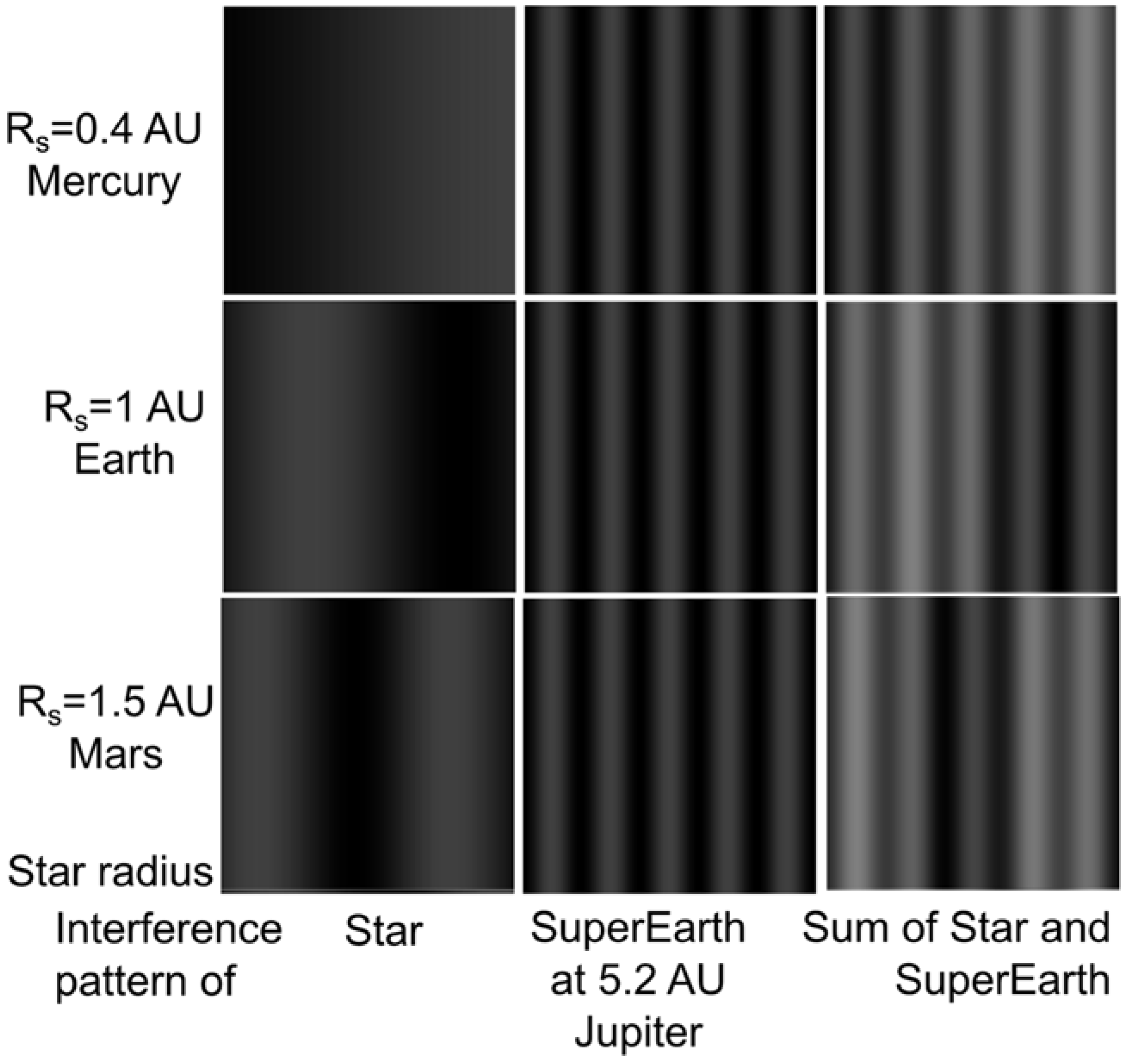
Nine simulation cases are presented in Figure 6, as an illustration of the effect of the distance of the star from the origin of the primed coordinate system. They are all interference patterns, calculated according to Equation (32). First the figure organization is explained.
The text in column 1 presents the displacement of the center of the red giant star. By analogy with our own solar systems, the location of the star center is assumed at 0.4 AU, 1 AU, and 1.5 AU, corresponding to the radius of the orbit of Mercury, Earth, and Mars. The second column features the interference pattern of the star with itself. The third column displays the interference pattern of the Super Earth planet with itself, for the specific case of the Jupiter distance of 5.2 AU. The fourth column features the sum of the interference patterns of the red-giant star and the Super Earth planet. The fourth row describes the images presented in each column above. The OPD within the interferometer arms is equal to half a wavelength.
The interesting trend that the reader is invited to appreciate here is the increasing number of the star fringes as the distance of the star center displacement increases from the coordinate origin. Similarly, as the star center displacement becomes smaller than the radius of the Mercury orbit, the red-giant star generates less than 0.5 fringe. This is basically the limiting distance of the star center that still produces an identifiable fringe. It represents a large error in the star position. This means that for relatively small errors, there is a negligibly small gradient in the observed star incidance. The interference pattern of the planet thus dominates the sum of the planet and the star incidance, with the star background contributing a clearly identifiable gradient.
The effects of the background incidance gradient becomes smaller with the decreasing alignment error. When the center of the red giant star is displaced to the Earth’s distance from the Sun, exactly one fringe is observed. Only a fraction of a fringe is observed when the red giant star is placed to the distance of the Mercury orbit. For nearer star locations, the partial star fringe looks like a slowly varying incidence field.
One may then conclude, that for most star alignment errors smaller than the radius of the Mercury orbit, even in the case of the red giants, Equation (26) simplifies to a constant background term and a sinusoidal modulation due to the planet.
The modulation is only present when there is a planet in the field of view. Furthermore, the fringe separation may be changed by changing the orientation of the Dove prism to verify the signal authenticity.
5. Summary
The theory of the detection of an extra-solar planet using a rotational shearing interferometer has been expanded to the case when this instrument is not precisely aligned on the star. For the small amounts of misalignment, the planet signal modulates the constant star signal. This finding was previously demonstrated for the case of the perfect alignment. For the relatively large displacement of the star from the origin, corresponding to the displacement equal to the Mercury orbit of 0.4 AU, some small variation in incidance may be detected with a high bit depth detector and subtracted. The relative change in incidance of the star fringe pattern due to the star displacement or misalignment may be estimated to be of the order of magnitude of the square of the misalignment angle in radians.
An interesting trend is noted that the increasing number of star fringes is generated when the distance of the star center increases from the coordinate origin. Similarly, as the displacement of the star center becomes smaller than the radius of the Mercury orbit, the red-giant star generated less than 0.5 fringe. The Mercury orbit could be considered as the limiting distance of the star center that still produces an identifiable fringe. It represents a large error in the star position, so one may safely conclude that for relatively small errors, a negligible gradient in the star incidance is observed. The interference pattern of the planet thus dominates the sum of the planet and the star incidance, with the star background contributing a small incidance gradient. The background incidance gradient decreases with the decreasing alignment error.
Alignment errors corresponding to the Mercury orbit are not expected in a process of bore-sighting on the star. If one accepts as reasonable errors those equal to the radius of a normal, main sequence star like our Sun, such errors do not result in discernable incidance changes. When a red giant star is considered and its potential displacement to the edge of its radius (nearly the Earth orbit), this indeed represents a significant error in alignment and would result in a formation of a star generated fringe. Then the image processing techniques may be used to separate the star incidance contribution from that of the planet.
For most star alignment errors appreciably smaller than the radius of the Mercury orbit, even in the case of the red giants, the detected incidance simplifies to a constant background term and a sinusoidal modulation. The modulation is only present when there is a planet in the field of view. Furthermore, the fringe separation may be changed by changing the orientation of the Dove prism to verify the signal veracity.
A large star misalignment corresponds to a star center location that is larger than the radius of the Martian orbit. Such a case may arise when a displaced star is found in the same field as the star of interest located on the optical axis. One may observe the star equal-gray-level fringe along a specific angle, while the equal gray-level fringe due to the planet is oriented along a different angle. This angle increases as the planet orbits the star. Finally, the planet fringes change orientation with respect to the star fringes during the local year, again introducing a useful temporal dependence.
Funding
The research described here was partially supported by the Air Force Office of Scientific Research, under contract No. (FA9550-18-1-0454).
Institutional Review Board Statement
Not applicable.
Informed Consent Statement
Not applicable.
Data Availability Statement
Not applicable.
Acknowledgments
A portion of this work was presented at the virtual conference Advances in 3OM Conference in Timisoara, Romania, December 2021.
Conflicts of Interest
The author declares no conflict of interest.
References
- NASA. How Many Exoplanets are There? Available online: https://exoplanets.nasa.gov/faq/6/how-many-exoplanets-are-there/ (accessed on 1 February 2022).
- Henry, G.W.; Marcy, G.W.; Butler, R.P.; Vogt, S.S. A transiting ‘51 peg-like’ planet. Astrophys. J. 2000, 529, L41–L44. [Google Scholar] [CrossRef] [PubMed] [Green Version]
- Charbonneau, D.; Brown, T.M.; Latham, D.W.; Mayor, M. Detection of Planetary Transits Across a Sun-like Star. Astrophys. J. Lett. 2000, 529, L45–L48. [Google Scholar] [CrossRef] [PubMed] [Green Version]
- Brown, T.M.; Charbonneau, D.; Gilliland, R.L.; Noyes, R.W.; Burrows, A. Hubble Space TelescopeTime-Series Photometry of the Transiting Planet of HD 209458. Astrophys. J. Lett. 2001, 552, 699–709. [Google Scholar] [CrossRef] [Green Version]
- Konacki, M.; Torres, G.; Sasselov, D.D.; Pietrzynski, G.; Udalski, A.; Jha, S.; Ruiz, M.T.; Gieren, W.; Minniti, D. The Transiting Extrasolar Giant Planet around the Star OGLE-TR-113. Astrophys. J. Lett. 2004, 609, L37–L40. [Google Scholar] [CrossRef] [Green Version]
- Mayor, M.; Queloz, D. A Jupiter-mass companion to a solar star. Nature 1995, 378, 355–359. [Google Scholar] [CrossRef]
- Butler, R.; Bedding, T.; Kjeldsen, H.; McCarthy, C.; O’Toole, S.; Tinney, C.; Marcy, G.; Wright, J. Ultra-high-precision velocity measurements of oscillations in alphacentauri A. Astrophys. J. 2004, 600, L75–L78. [Google Scholar] [CrossRef] [Green Version]
- Kubas, D.; Cassan, A.; Beaulieu, J.P.; Coutures, C.; Dominik, M.; Albrow, M.D.; Brillant, S.; Caldwell, J.A.R.; Dominis, D.; Donatowicz, J.; et al. Full characterization of binary-lens event OGLE-2002-BLG-069 from PLANET observations. Astron. Astrophys. 2005, 435, 941–948. [Google Scholar] [CrossRef] [Green Version]
- Schultz, A.; Schroeder, D.; Jordan, I.; Bruhweiler, F.; DiSanti, M.; Hart, H.; Hamilton, F.; Hershey, F.; Kochte, M.; Miskey, C.; et al. Imaging planets about other stars with UMBRAS. In Infrared Spaceborne Remote Sensing VII; SPIE: Bellingham, WA, USA, 1999; Volume 3759. [Google Scholar]
- Scholl, M.S. Apodization effects due to the size of a secondary mirror in a reflecting, on-axis telescope for detection of Extra-solar planets. In Infrared Spaceborne Remote Sensing; SPIE: Bellingham, WA, USA, 1993; Volume 2019. [Google Scholar] [CrossRef]
- Queloz, D.; Eggenberger, A.; Mayor, M.; Perrier, C.; Beuzit, J.L.; Naef, D.; Sivan, J.P.; Udry, S. Detection of a spectroscopic transit by the planet orbiting the star HD209458. Astron. Astrophys. 2000, 359, L13–L17. [Google Scholar]
- Richardson, L.J.; Deming, D.; Horning, K.; Seager, S.; Harrington, J. A spectrum of an extrasolar planet. Nature 2007, 445, 892–895. [Google Scholar] [CrossRef]
- Wright, J.T.; Upadhyay, S.; Marcy, G.W.; Fischer, D.; Ford, E.B.; Johnson, J.A. Ten New and Updated Multiplanet Systems and a Survey of Exoplanetary Systems. Astrophys. J. Lett. 2001, 693, 1084–1089. [Google Scholar] [CrossRef] [Green Version]
- Neuhäuser, R.; Guenther, E.W.; Wuchterl, G.; Mugrauer, M.; Bedalov, A.; Hauschildt, P.H. Evidence for a co-moving sub-stellar companion of GQ Lup. Astron. Astrophys. 2005, 435, L13–L16. [Google Scholar] [CrossRef]
- Moutou, C.; Mayor, M.; Curto, G.; Ségransan, D.; Udry, S.; Bouchy, F.; Benz, W.; Lovis, C.; Naef, D.; Pepe, F.; et al. The HARPS search for southern extra-solar planets XXVIII. Seven new planetary systems. Astrophys. J. 2011, 527, A63. [Google Scholar]
- Scholl, M.S. Star-Light Suppression with a Rotating Rotationally-Shearing Interferometer for Extra-Solar Planet Detection in Signal Recovery and Synthesis; 1995 OSA Technical Digest Series; Optica: Washington, DC, USA, 1995; Volume 11, pp. 54–57. [Google Scholar]
- Scholl, M.S. Signal detection by an extra-solar-system planet detected by a rotating rotationally-shearing interferometer. J. Opt. Soc. Am. A 1996, 13, 1584–1592. [Google Scholar] [CrossRef]
- Butler, R.P. Other Planetary Systems. In The New Solar System; Beatty, J.K., Petersen, C.C., Chaikin, A., Eds.; Cambridge University Press: Cambridge, UK, 1999; pp. 377–386. [Google Scholar]
- De Pater, I.; Lissauer, J.J. Planetary Sciences; Cambridge University Press: Cambridge, UK, 2001. [Google Scholar]
- Alonso, R.; Brown, T.M.; Torres, G.; Latham, D.W.; Sozzetti, A.; Mandushev, G.; Belmonte, J.A.; Charbonneau, D.; Deeg, H.J. TrES-1: The transiting planet of a bright K0 V star. Astrophys. J. 2004, 613, L153–L156. [Google Scholar] [CrossRef]
- Fischer, D.A.; Laughlin, G.; Butler, P.; Marcy, G.; Johnson, J.; Henry, G.; Valenti, J.; Vogt, S.; Ammons, M.; Robinson, S.; et al. The N2K consortium. I. A hot saturn planet orbiting HD 881331. Astrophys. J. 2005, 620, 481–486. [Google Scholar] [CrossRef] [Green Version]
- Wall, M. 1,000 Alien Planets! NASA’s Kepler Space Telescope Hits Big Milestone. Available online: http://www.space.com/28105-nasa-kepler-spacecraft-1000-exoplanets.html (accessed on 14 November 2021).
- Strojnik, M.; Kirk, M.S. Telescopes. In Fundamentals of Basic Optical Instruments; Malacara, D., Thompson, B., Eds.; CRC Press: Boca Raton, FL, USA, 2017. [Google Scholar]
- Dunham, E.W.; O’Donovan, F.T.; Stefanik, R.P.; Dumusque, X.; Pepe, F.; Lovis, C.; Ségransan, D.; Sahlmann, J.; Benz, W.; Bouchy, F.; et al. An Earth-mass planet orbiting α Centauri B. Nature 2012, 491, 207–211. [Google Scholar]
- Lacour, S.; Nowak, M.; Wang, J.; Pfuhl, O.; Eisenhauer, F.; Abuter, R.; Amorim, A.; Anugu, N.; Benisty, M.; Berger, J.P.; et al. First direct detection of an exoplanet by optical interferometry Astrometry and K-band spectroscopy of HR 8799 e. Astron. Astrophys. 2019, 623, L11. [Google Scholar]
- Strojnik, M.; Bravo-Medina, B. Extra-solar planet detection methods. In Infrared Remote Sensing and Instrumentation XXVI; SPIE: Bellingham, WA, USA, 2018; Volume 10765, p. 107650Y. [Google Scholar] [CrossRef]
- Scholl, M.S. Infrared signal generated by a planet outside the solar system discriminated by rotating rotationally-shearing interferometer. Infr. Phys. Technol. 1996, 37, 307–312. [Google Scholar] [CrossRef]
- Strojnik, M. Comparison of linear and rotationally shearing interferometric layouts for extrasolar planet detection from space. Appl. Opt. 2003, 42, 5897–5905. [Google Scholar] [CrossRef]
- Strojnik, M. Simulated interferometric patterns generated by a nearby star-planet system and detected by a rotationally-shearing interferometer. J. Opt. Soc. Am. A 1999, 16, 2019–2024. [Google Scholar] [CrossRef]
- Strojnik-Scholl, M. Cancellation of star-light generated by a nearby star-planet system upon detection with a rotationally-shearing interferometer. Infr. Phys. Technol. 1999, 40, 357–365. [Google Scholar] [CrossRef]
- Scholl, M.S. Versatility of the differential rotationally-shearing interferometer for testing the aspherical surfaces. In Optical Fabrication and Testing (OFT’98); OSA Technical Digest Series; Optical Society of America: Washington, DC, USA, 1998. [Google Scholar]
- Strojnik, M. Interferometry to Detect Planets Outside Our Solar System. In Interferometry Applications in Topography and Astronomy; Padron, I., Ed.; InTech Pub. Co.: Rijeka, Croatia, 2012; pp. 195–220. ISBN 978-953-51-0404-9. [Google Scholar]
- Strojnik, M. Extrasolar planet observatory on the far side of the Moon. J. Appl. Remote Sens. 2014, 8, 084982. [Google Scholar] [CrossRef] [Green Version]
- Strojnik, M.; Bravo-Medina, B. Rotationally shearing interferometer for extra-solar planet detection: Preliminary results with a solar system simulator. Opt. Express 2020, 28, 29553–29561. [Google Scholar] [CrossRef]
- Strojnik, M. Rotationally shearing interferometry in the recovery of faint signals. In Infrared Remote Sensing and Instrumentation XXIX; SPIE: Bellingham, WA, USA, 2021; Volume 11830, p. 1183007. [Google Scholar] [CrossRef]
- Gutierrez, E.; Strojnik, M. Interferometric tolerance determination for a Dove prism using exact ray trace. Opt. Commun. 2008, 281, 897–905. [Google Scholar] [CrossRef]
- Gutierrez, E.; Strojnik, M. Quantification of critical alignment parameters for a rotationally-shearing interferometer employing exact ray trace. J. Mod. Opt. 2010, 57, 444–459. [Google Scholar] [CrossRef]
- Moreno, I.; Strojnik, M. Dove prism with increased throughput for implementation in rotational shearing interferometer. Appl. Opt. 2003, 42, 4514–4521. [Google Scholar] [CrossRef]
- Moreno, I.; Strojnik, M. Polarization transforming properties of Dove prisms. Opt. Commun. 2003, 220, 257–268. [Google Scholar] [CrossRef]
- Moreno, I.; Strojnik, M. Reversal and rotationally shearing interferometer. Opt. Commun. 2004, 233, 245–252. [Google Scholar] [CrossRef]
- Gonzalez-Romero, R.; Strojnik, M.; Garcia-Torales, G. Theory of a rotationally shearing interferometer. JOSA-A 2021, 38, 264–270. [Google Scholar] [CrossRef]
- Strojnik, M.; Scholl, M.K. Radiometry. In Advanced Optical Instruments and Techniques; Malacara, D., Thompson, B., Eds.; CRC Press: New York, NY, USA, 2018; pp. 459–717. ISBN1 978-1-49872-067-0. ISBN2 978-1-31511-997-7. [Google Scholar]
Figure 1.
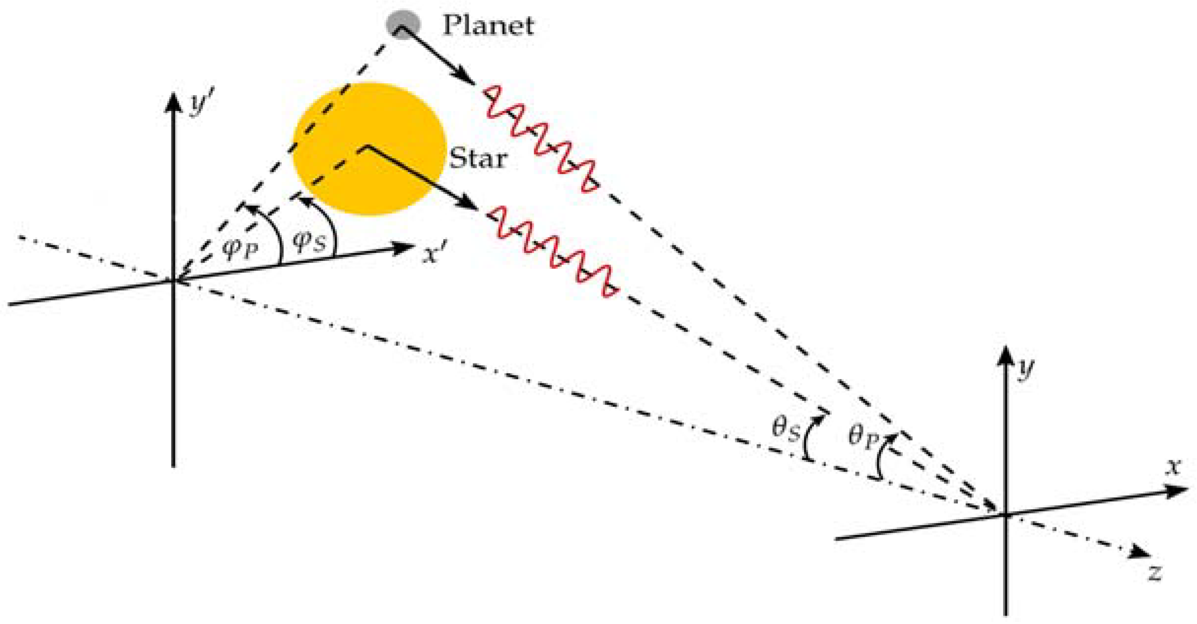
Star-planet system in x′-, y′- coordinate system, viewed from the rotational shearing interferometer at the origin of coordinate system (x,y,z) on or near the Earth. The star and the planet may be modeled as point sources with an elevation-angle, θ (measured from the negative optical axis), and an azimuth-angle, φ, with respect to the x′- axis. The planet quantities have a subscript P, those of the star have S. The star coordinates correspond to the alignment error. The planet coordinates are unknown because it is invisible.
Figure 1.
Star-planet system in x′-, y′- coordinate system, viewed from the rotational shearing interferometer at the origin of coordinate system (x,y,z) on or near the Earth. The star and the planet may be modeled as point sources with an elevation-angle, θ (measured from the negative optical axis), and an azimuth-angle, φ, with respect to the x′- axis. The planet quantities have a subscript P, those of the star have S. The star coordinates correspond to the alignment error. The planet coordinates are unknown because it is invisible.

Figure 2.
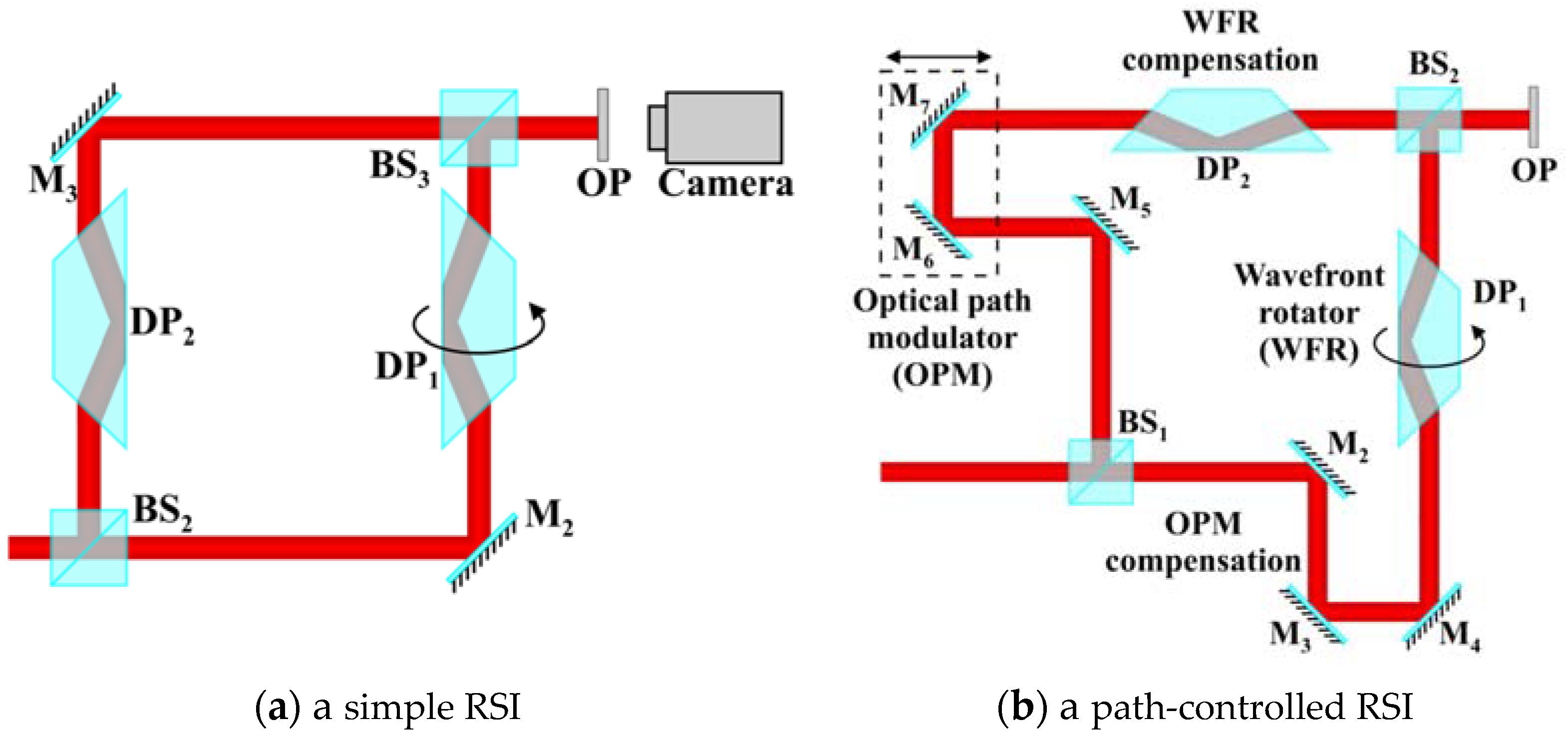
(a) An RSI implemented in a Mach–Zehnder configuration with two Dove prisms. A Dove prism DP that is rotated by an angle about the optical axis introduces the wavefront shear in the RSI. The symbols are interpreted as follows: M, mirror; BS, beam splitter; and OP, observation plane. (b) Conceptual design of an RSI with an electro-opto-mechanical delay module in one arm and a compensation module in the other arm. A computer-controlled two-mirror assembly in each arm is used to precisely adjust the paths in both interferometer arms for increased wavefront coherence.
Figure 2.
(a) An RSI implemented in a Mach–Zehnder configuration with two Dove prisms. A Dove prism DP that is rotated by an angle about the optical axis introduces the wavefront shear in the RSI. The symbols are interpreted as follows: M, mirror; BS, beam splitter; and OP, observation plane. (b) Conceptual design of an RSI with an electro-opto-mechanical delay module in one arm and a compensation module in the other arm. A computer-controlled two-mirror assembly in each arm is used to precisely adjust the paths in both interferometer arms for increased wavefront coherence.

Figure 3.
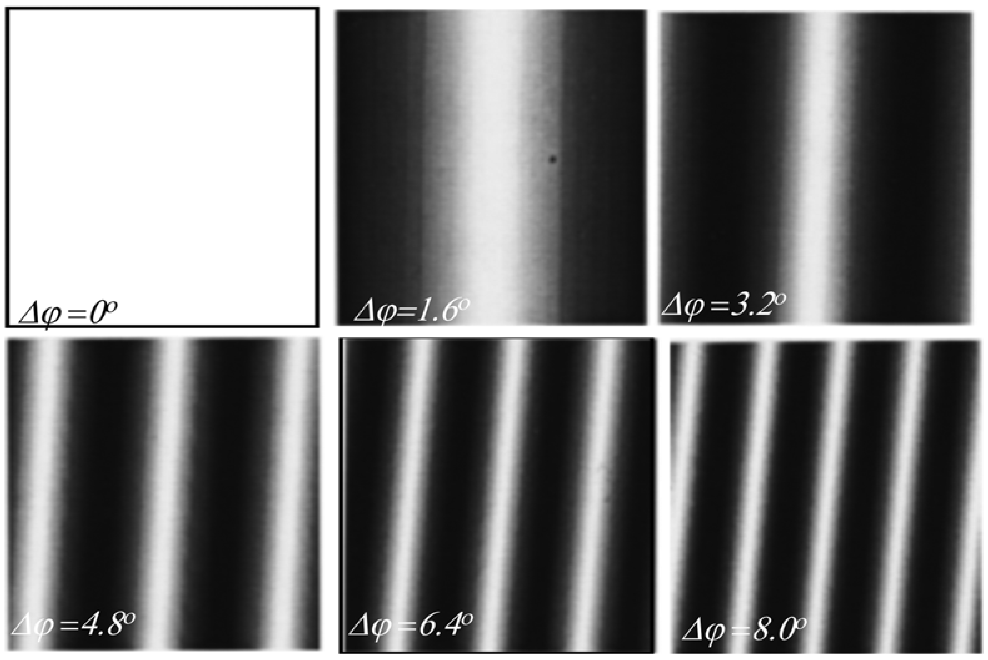
Interference fringes of tilt simulated in an RSI when the shear angle is increased from 0°- rotation angle (blank field) to 8° in increments of 1.6° (axis of rotation is normal to the page). The shear angle is the angle of the orientation of the Dove prism, or the wavefront rotator in Figure 2. The density of fringes increases, and the fringe inclination angle decreases with increasing wavefront rotation angle. The fringe angle is defined as the angle that the straight line through the bright fringe makes with the horizontal axis.
Figure 3.
Interference fringes of tilt simulated in an RSI when the shear angle is increased from 0°- rotation angle (blank field) to 8° in increments of 1.6° (axis of rotation is normal to the page). The shear angle is the angle of the orientation of the Dove prism, or the wavefront rotator in Figure 2. The density of fringes increases, and the fringe inclination angle decreases with increasing wavefront rotation angle. The fringe angle is defined as the angle that the straight line through the bright fringe makes with the horizontal axis.

Figure 4.
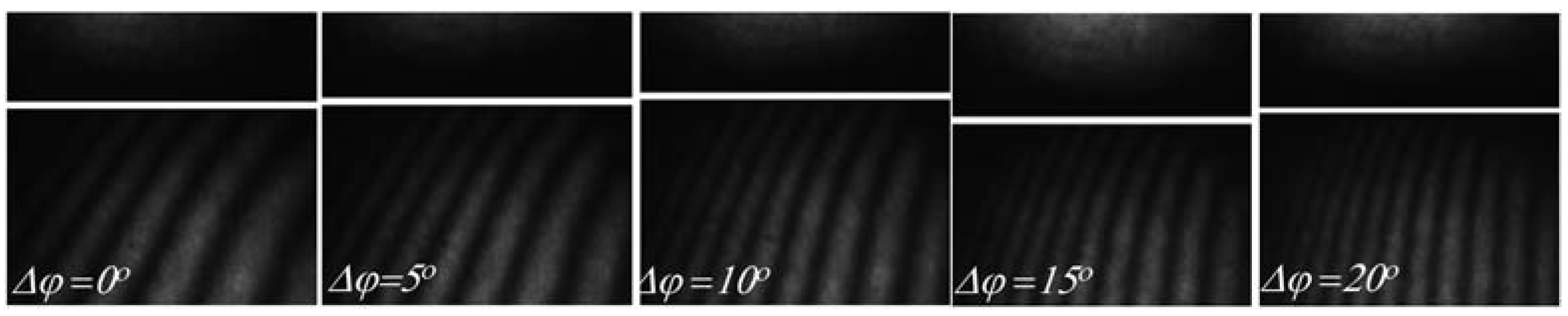
Experimentally obtained interference patterns indeed change when the angle of orientation of the Dove prism increases from 0 to 20° for an off-axis point source. The nearly straight interference fringes increase in density and increase in the inclination angle when the shear angle is increased in increments of 5°. This is one of the characteristics of the RSI in measuring the tilted wave fronts, such as those originating at an off-axis planet. This experimental data confirms that an off-axis source can be detected in an RSI by generating straight fringes. Furthermore, the fact that the fringes arise from an off-axis source, rather than because of an artifact, may be confirmed by changing the shear angle and observing how their density and angle of inclination change.
Figure 4.
Experimentally obtained interference patterns indeed change when the angle of orientation of the Dove prism increases from 0 to 20° for an off-axis point source. The nearly straight interference fringes increase in density and increase in the inclination angle when the shear angle is increased in increments of 5°. This is one of the characteristics of the RSI in measuring the tilted wave fronts, such as those originating at an off-axis planet. This experimental data confirms that an off-axis source can be detected in an RSI by generating straight fringes. Furthermore, the fact that the fringes arise from an off-axis source, rather than because of an artifact, may be confirmed by changing the shear angle and observing how their density and angle of inclination change.

Figure 5.
A solar system, that includes a Sun-like star and a Jupiter-like planet at 10 parsecs, subtends an angle of 2 μrad at the Earth. At that distance, the star and the planet subtend an angular radius of 10−4 and 10−5 μrad at the Earth. Due to the resolution limitations of the available telescopes, both the planet and the star are unresolved, or point, sources.

Figure 6.
An illustration of the effect of the distance of the star center from the origin of the primed coordinate system (see Figure 1). The text in column 1 presents the displacement of the center of the red giant star. The star centers are located at 0.4 AU, 1 AU and 1.5 AU distances from the coordinate origin. The second column features the interference patterns of the star with itself for three star-center positions. The third column displays the interference pattern of the Super Earth planet with itself, for the specific case of the Jupiter distance of 5.2 AU. The fourth column features the sum of the interference patterns of the red-giant star and the Super Earth planet. The planet interference pattern dominates the sum of the planet and the star incidances.

Publisher’s Note: MDPI stays neutral with regard to jurisdictional claims in published maps and institutional affiliations. |
© 2022 by the author. Licensee MDPI, Basel, Switzerland. This article is an open access article distributed under the terms and conditions of the Creative Commons Attribution (CC BY) license (https://creativecommons.org/licenses/by/4.0/).
Share and Cite
MDPI and ACS Style
Strojnik, M. Rotational Shearing Interferometer in Detection of the Super-Earth Exoplanets. Appl. Sci. 2022, 12, 2840. https://0-doi-org.brum.beds.ac.uk/10.3390/app12062840
AMA Style
Strojnik M. Rotational Shearing Interferometer in Detection of the Super-Earth Exoplanets. Applied Sciences. 2022; 12(6):2840. https://0-doi-org.brum.beds.ac.uk/10.3390/app12062840
Chicago/Turabian StyleStrojnik, Marija. 2022. "Rotational Shearing Interferometer in Detection of the Super-Earth Exoplanets" Applied Sciences 12, no. 6: 2840. https://0-doi-org.brum.beds.ac.uk/10.3390/app12062840
Note that from the first issue of 2016, this journal uses article numbers instead of page numbers. See further details here.