
Optomechanical Analysis and Design of Polygon Mirror-Based Laser Scanners


1
3OM Optomechatronics Group, Faculty of Engineering, “Aurel Vlaicu” University of Arad, Str. Elena Dragoi No. 2, 310177 Arad, Romania
2
Doctoral School, Polytechnic University of Timisoara, 1 Mihai Viteazu Avenue, 300222 Timisoara, Romania
3
School of Science and Engineering, University of Groningen, W.F. Bathoornstraat, 9731 CG Groningen, The Netherlands
*
Author to whom correspondence should be addressed.
Appl. Sci. 2022, 12(11), 5592; https://0-doi-org.brum.beds.ac.uk/10.3390/app12115592
Submission received: 9 May 2022
/
Revised: 27 May 2022
/
Accepted: 27 May 2022
/
Published: 31 May 2022
(This article belongs to the Special Issue Progress in 3OM: Opto-Mechatronics, Opto-Mechanics, and Optical Metrology)
Abstract
:Featured Application
Applications of polygon mirror-based scanning heads include laser scanning, 2D and 3D printing, laser manufacturing, imaging, optical metrology, and Remote Sensing.
Abstract
Polygon Mirror (PM)-based scanning heads are one of the fastest and most versatile optomechanical laser scanners. The aim of this work is to develop a multi-parameter opto-mechanical analysis of PMs, from which to extract rules-of-thumbs for the design of such systems. The characteristic functions and parameters of PMs scanning heads are deduced and studied, considering their constructive and functional parameters. Optical aspects related to the kinematics of emergent laser beams (and of corresponding laser spots on a scanned plane or objective lens) are investigated. The PM analysis (which implies a larger number of parameters) is confronted with the corresponding, but less complex aspects of Galvanometer Scanners (GSs). The issue of the non-linearity of the scanning functions of both PMs and GSs (and, consequently, of their variable scanning velocities) is approached, as well as characteristic angles, the angular and linear Field-of-View (FOV), and the duty cycle. A device with two supplemental mirrors is proposed and designed to increase the distance between the GS or PM and the scanned plane or lens to linearize the scanning function (and thus to achieve an approximately constant scanning velocity). These optical aspects are completed with Finite Element Analyses (FEA) of fast rotational PMs, to assess their structural integrity issues. The study is concluded with an optomechanical design scheme of PM-based scanning heads, which unites optical and mechanical aspects—to allow for a more comprehensive approach of possible issues of such scanners. Such a scheme can be applied to other types of optomechanical scanners, with mirrors or refractive elements, as well.
1. Introduction
Laser scanners can be roughly divided in systems with or without moving parts [1,2,3]. The first category includes the most common Galvanometer Scanners (GSs) [3,4,5,6,7,8,9,10,11,12,13], Polygon Mirrors (PMs), in various configurations (i.e., prismatic or pyramidal, normal or inverted, regular or irregular) [14,15,16,17,18,19,20,21,22,23,24,25,26,27,28,29,30,31,32,33,34,35], holographic scanners [2], as well as devices with refractive elements (i.e., lenses [36] or prisms [37,38,39,40,41,42]). The second category includes electro- or acousto-optical scanners, which have the clear advantage of no mechanical inertia, therefore a much higher positioning velocity than the first category [2]. However, they have the drawback of a lower scanning resolution [1,2], and this makes them less attractive, especially for high-end applications such as biomedical imaging—including Optical Coherence Tomography (OCT) [43,44,45,46,47,48,49] and Confocal Microscopy (CM) [50].
Each system in the first category (i.e., of optomechanical scanners) has different advantages and drawbacks that makes it more suitable for a certain application. Broadly, in the competition between scanners with reflective and refractive elements, the former usually win, because of a higher versatility in terms of spectral range, as well as fewer aberration and dispersion issues. An exception could be made by Risley prisms scanners, because of their high positioning precision and velocity for two-dimensional (2D) scanning [37,38,39,40,41,42], but in general, mirror-based systems (i.e., GSs and PMs) are the most common for the largest range of applications because of the above advantages [1,2,3,4].
Within this latter narrower category, in the 1990s, the GSs seemed to take over the field almost completely because of their overall good characteristics, which include high positioning precision at a large Field-of-View (FOV) and good resolutions at satisfactory scanning velocities, all achieved in compact, light-weight constructions, and at a reasonable cost per scan axis. However, PMs seemed to make quite a comeback starting in the early 2000s because of their particular advantage: High scanning velocity. With the necessity to develop broadband laser sources scanned in frequency for Swept Source (SS) OCT [44], PMs caught the attention of both research [19,20,21,22,23,24,25,26] and technological development [51]. Various SS configurations have been developed, with on-axis [19] and off-axis PMs [20], as well as telescope [19,20,21,22] and telescope-less, the latter in Littrow [23], Littman [24], and Littrow–Littman [25] setups. One of the most critical features of PM scanners for today’s applications, i.e., the maximum limit of their rotational velocity (ω), has been approached by the industry. Thus, high-end PM scanners have rotational motors that commonly reach 54 krpm and even 70 krpm, while developments to reach 120 krpm exist. This results in scan frequencies (fs) equal to this rotational frequency multiplied by the number of PM facets. This pushes forward the design of motors and (especially aerodynamic) bearings, as well as fast and robust sensors and control structures. It also imposes performing a Finite Element Analysis (FEA) for each particular design, to assess the structural integrity and level of deformations, as highlighted in the literature [1]. Another direction of research in the scanners field, especially in the last decade, is related to handheld scanning probes (for example, for OCT [52,53,54,55,56,57]), and scanning heads in general (for applications such as 3D printing or laser manufacturing [58,59,60]). While the former usually implies GSs or Micro-Electro-Mechanical Systems (MEMS), the latter also utilizes PM plus GS 2D systems to increase scanning velocity, and therefore productivity in industrial processes, for example.
Starting from the necessity to clarify their fundamental characteristics, the basis of a theory regarding the optical functions and parameters of PM scanning heads has been approached in a preliminary study [32], based on a series of previous works [28,29,30,31]. The focus has been to develop a theory that is both simple to use and rigorous, in the context of valuable but rather complex existing approaches [1,14,15,16,17]. PM-based SSs optimization is one of its field of interest [26], but the preliminary theory developed in [32] has raised interest for other applications as well, such as additive manufacturing/3D printing. In [35], for example, the functions developed in [32] were applied by using the suggestion made regarding the capability of the theory to pass from single rays to finite diameter laser beams, as we aim to complete in the present study. Moreover, in [61,62] steps have been taken to develop monogon-type PMs with a curved facet to avoid using an objective lens, by linearizing PM scanning functions starting from the study and equations in [32].
Another motivation of the present study is the necessity to better unite optical analysis and design with other essential PM issues, such as mechanical ones, as pointed out in the literature [1]. Such mechanical (but also electrical and control) aspects of PM scanners are usually left to manufactures, to come with as-good-as-possible solutions between various (and commonly contradictory) aspects of scanner analysis and design.
Therefore, the aim of the present work is to study optical aspects of PMs, which are essentially related to the kinematics of the laser beam, but also to relate them to mechanical issues. The latter is performed through a multi-parameter FEA that must consider constructive elements of the system. A limitation of the present work in this respect is the fact that only examples of these parameters are considered, as the scope is not to complete an exhaustive FEA (for all possible configurations, materials, and dimensions of PMs), but to develop connections of optical and mechanical aspects in order to complete both an analysis and design methodology of such scanners. Another limitation is not approaching control and automation aspects of the PMs, with their fast motors, because this is an entirely different topic, as in the case of GSs [11,12,13].
Finally, one must point out that, similar to scanners with oscillatory elements, the work completed on macro-devices can be applied, at least in part, to MEMS, as shown in the case of GSs [10]. Therefore, the development of an as comprehensive and rigorous as possible analysis and design of macro-PMs can be of interest in the context of the tendency to miniaturize optical and laser systems, for example, in endoscopes (to enter body lumens) [63,64,65], but also in other areas where a decrease in mass and dimensions is a critical aspect, as in Remote Sensing or Security and Defense.
The remainder of this paper includes, in Section 2, the presentation of the two considered scanning systems, with their principles and constructive parameters. Their functions and parameters are obtained, in a parallel between PMs and GSs. In Section 3, the multi-parameter analysis of the two scanners is performed, for their deduced functions. In Section 4, a solution to linearize the scanning function (and thus to obtain approximately constant scanning velocities) is developed. Section 5 presents the performed FEA of PMs, while Section 6 unites these two aspects, optical and mechanical, in a single design scheme. Section 7 provides conclusions, as well as directions of future work.
2. Characteristic Functions and Parameters of PMs versus GSs
2.1. GSs and PM Scanning Heads
The schematics of 1D GSs and of PM-based scanning heads are presented in Figure 1 and Figure 2, respectively.
GSs have a mirror mounted on the mobile element (i.e., on the shaft of its electric motor) that performs oscillatory movements with a certain angular amplitude θm (of up to 30° for modern devices [1,2,3,4,58,59,60])—Figure 1a.
In contrast, PMs perform a continuous rotational movement—Figure 2a. This gives the PMs the advantages of a much higher scanning velocity and of a one-direction scan, which is important, for example, for SSs [19,20,21,22,23,24,25,26] and for lateral scanning in imaging, for example, with CM or OCT [43,44,45,46,47,48,49,50].
The GS oscillatory mirror must stop and turn, which is where mechanical inertia comes into play, therefore its deceleration and acceleration periods cannot provide a constant scanning velocity v—Figure 1b. This proves to be a major drawback. Thus, for the most common triangular and sawtooth input signals of the device, non-linearities occur in the corresponding time intervals (Δt in the example in Figure 1c for triangular signals). This phenomenon was demonstrated and studied in detail in [7], with examples of galvoscanning in OCT. For such imaging methods, it means that the corresponding distorted portions (i.e., with non-equally spaced pixels) must be discarded, as performed in [8] based on the study in [7]. This reduces the useful angular scan amplitude from θm to θa, and the useful linear scanning field (i.e., the one scanned with constant velocity), from 2H to 2xa—Figure 1a. In consequence, the duty cycle (i.e., the time efficiency of the scanning process) decreases as well—as modelled mathematically in [9] to perform collations of individual GS-based OCT images. Thus, (larger) mosaic images can be obtained, to reach a higher FOV than the one for individual scans.
For other common, sinusoidal inputs applied to the GS, the scan is performed with variable velocity over the entire FOV, therefore the duty cycle is even lower than for triangular or sawtooth scanning, as only a small portion of the characteristic can be considered approximately linear. In fact, the entire scan (i.e., the image in the case of CM or OCT) is distorted and must be post-processed, and this can produce artefacts. On the other hand, sinusoidal inputs have the advantage of a smoother mechanical regime, therefore the maximum scan frequency fs is higher than for sawtooth scanning, for example, as indicated by manufacturers [58,59,60].
Finally, there is a clear trade-off for GSs between fs and θm: As modelled from experimental data [7,9,10], the maximum possible/limit scan amplitude (i.e., the one that still corresponds to a controlled and not to a chaotic movement of the mobile element) drops almost exponentially with fs, therefore one cannot utilize the higher fs of GSs for a larger FOV [10]; the FOV is significantly reduced for fs close to the maximum value of 1 kHz that is specific to a GS with an aperture of around 4 mm used in OCT or CM, for example [58]. For other applications where GSs of different apertures are utilized (higher, as in laser manufacturing, for example [60]), the values of such limits and dependences are different, but the phenomenon is similar [10].
In contrast, for PMs, the FOV is constant and irrespective of the rotational velocity, but dependent on the dimensions of the PMs. The latter are determined in the literature using a simple, common design algorithm that addresses the calculus of fs [1], as discussed in Section 6.
In terms of geometrical parameters, GSs are characterized by the mirror aperture and the distance L from the mirror pivot O (which is commonly the incidence point of the incoming laser beam) to the scanned plane or lens. In the latter case, L is equal to the object focal distance f of the lens, as shown in Figure 1a.
In contrast, PMs have three more main geometrical parameters: R, the apothem of the polygon; e, the eccentricity of the fixed incident laser beam from the pivot O; n, the number of PM facets, which gives the angle that corresponds to half of a PM facet, α = π/n—Figure 2a. Other constructive parameters of PMs in Figure 2a, such as facet width a and thickness b, are necessary only for the FEA (and not for the optical analysis), therefore they are considered only in Section 5 and Section 6.
As, in general, an objective lens is utilized for both setups (with GS or PM), both scanners are also characterized by its diameter D (or aperture in the meridian plane Oyz).
In most of this study, to simplify the mathematical discussion, only the axis of the laser beam is considered, therefore it is as if the beam is reduced to its center ray, a situation that may roughly correspond to a well-collimated laser beam. We return to this simplifying hypothesis in Section 3, where a finite diameter 2ρ of the beam is considered, as well. The advantage of the theory to be developed is that, as observed from Figure 2b, a variation of the eccentricity e can consider this beam radius ρ in the equations to be deduced, as demonstrated further on in Section 3.5.
2.2. Characteristic Functions of GSs and PM Scanning Heads
From the point of view of the movement of the reflected/emergent laser beam (and of the corresponding spot on a scanned plane or objective lens), both types of scanners are characterized by several functions, as pointed out in Figure 1b and Figure 2b:
(i) The scanning function h(θ) is defined by the (current) position of the laser spot on the scanned plane/lens or of the laser beam emerging the lens with regard to its optical axis (O.A.).
To allow for a comparison of GS and PM scanning heads, the O.A. of both scanners is considered perpendicular on the fixed incident laser beam, in a common setup utilized in numerous applications [1]. Furthermore, to allow for a comparison of the functions of the two systems, the θ = 0 position is considered for a horizontal position of the GS mirror, as well as for a horizontal PM facet (i.e., for the PM apothem on the vertical axis Oζ)—Figure 2b.
(ii) The scanning velocity v(t) = dh/dt represents the sweeping velocity of the laser beam on the scanned plane or in the image space of the lens.
(iii) The scanning acceleration a(t) = dv/dt represents the acceleration of the laser beam in the scan direction—perpendicular on the O.A.
For the GS, the condition of having the reflected beam permanently parallel to the O.A. (i.e., with both v(t) and a(t) perpendicular to the beam emerging the lens) is fulfilled by placing the pivot O in the object focal point of the lens. For the PM, this condition can be fulfilled only approximately, as discussed in Section 2.3, but it also represents the desired aspect.
These three functions are obtained for a GS from Figure 1b and for a PM scanning head from Figure 2b:
- For a GS, the start position of the GS mirror is at π/4 [rad] with regard to the horizontal axis Oz. As the mirror rotates with θ, the reflected beam rotates with 2θ, therefore the scanning function would be h(θ) = L·tan2θ. While this simple equation is usually utilized for GSs [7,9,10], in the present study, to allow for a comparison to PMs, the θ = 0 position is considered for a horizontal position of the GS mirror (when the reflected beam would be superposed to the incident one), as previously pointed out. In this case, the scanning function results in being h(θ) = −L/tan2θ, therefore the scanning velocity and acceleration have Equations (2) and (3), respectively (Table 1). The graphs of these three functions are presented in Figure 3a.
- For a PM scanning head, a facet is represented in three positions in Figure 2b, considering θ = 0 for the facet in a horizontal position. Similar to GSs, the rotational angle θ = π/4 defines the facet position in which the (fixed vertical) incident beam is reflected on the (horizontal) Oz axis, which defines the O.A. of the lens. For θ1 and θ2 (with θ1 < π/4 < θ2), the reflected beam reaches the inferior and superior margins of the lens in the meridian plan Oyz, therefore h(θ1,2) = H (where H < D/2), Figure 2. Points P1, M, and P2 are the intersections of the incident ray with the PM facet for these three rotation angles considered (i.e., θ1, π/4, and θ2, respectively). For a current rotational angle θ, from Appendix A, the scanning function is deduced, with Equation (4), therefore the scanning velocity and acceleration are obtained with Equations (5) and (6), respectively (Table 1). An experimental validation of this PM scanning function was completed in [32].
- The comparison of each corresponding pair of functions (i.e., for GSs and PMs) is performed in Figure 3b, on a numerical example with L = 40 mm, R = 15 mm, e = 6 mm, and ω = 10 krpm (the latter corresponding to an idle rotation of the PM). The asymmetry of the PM functions graphs can be remarked, in comparison to the symmetry of (dotted graphs of) GS functions—to be discussed in Section 3.
2.3. Migration Functions
One can observe, from the expressions of the scanning function, velocity, and acceleration of PMs versus GS in Table 1, the supplemental terms in each PM function. They complicate the discussion, but also offer more degrees-of-freedom in the design process of a PM scanning head, which is an advantage. Thus, in [28,29,32], a novel concept has been introduced, of migration functions, transversal and longitudinal/axial . They have, from Figure 2b, Equations (7) and (8), respectively (Table 1). The former represents the coordinate of the incidence point P (of the beam on a PM facet), while the latter represents the coordinate of the axial point A from which it is as if the beam incident on the lens starts. Their graphs are obtained in Figure 4.
2.4. Scan Angles and Angular FOV
The two (different) pairs of characteristic scan angles of each system are marked on the graphs in Figure 3:
- For a GS, shown in Figure 1a, the total rotational angles interval is [π/2 − θm, θm] (Equation (9), Table 1) and the useful rotational angles interval is [π/2 − θa, θa] (Equation (10), Table 1), with the latter corresponding to the portion scanned with constant velocity [9,10]. Therefore, the angular FOV could be considered with either its useful value, 2θa − π/2, or with its total one, 2θm − π/2, Equation (11), Table 1.
- For a PM, two pairs of scan angles are important: θ1 and θ2, which define the useful angular FOV, as discussed in Section 2.2—Figure 2a,b; θmin and θmax, which define the down-reflected and up-deflected positions of the reflected beam of a scanner (in a concept introduced by Beiser [2]), therefore the total possible FOV—Figure 5a. To characterize these latter beams for a PM, we introduced the construction in Figure 5a [29,32], where the reflection is considered at the beginning and end of a PM facet (without referring to the vignetting produced by the finite beam diameter). From this figure, these two reflected beams are characterized bytherefore the expressions of the two (extreme) scanning angles are given by Equation (12), Table 1. These equations also give the total angular FOV of the PM—Equation (14), Table 1. The values of the useful angles θ1 and θ2 are obtained by solving Equation (13), Table 1.
Figure 5.
Rotational angles of the PM, θmin and θmax for which the ray reaches the margins of a PM facet: (a) The up- and down-deflected rays; (b) the two surfaces of the scan angles θmin and θmax for the (most useful) x < 1 and α < π/4 intervals with regard to these two parameters.
Figure 5.
Rotational angles of the PM, θmin and θmax for which the ray reaches the margins of a PM facet: (a) The up- and down-deflected rays; (b) the two surfaces of the scan angles θmin and θmax for the (most useful) x < 1 and α < π/4 intervals with regard to these two parameters.

2.5. Linear FOV
- For a GS, using Equation (1), the linear FOV (i.e., the maximum dimension that can be scanned on a certain target plane/lens) is obtained, with Equation (15), Table 1.
2.6. Duty Cycle
The duty cycle of a scanner is defined as its time efficiency, i.e., the ratio of the useful time (for the scanning process) and the total considered time interval. Essentially, this parameter is related to the scan angles above, but also to the specific structure (and application) of the scanner:
- For a GS, the duty cycle cannot be, for example, (as one may consider at a rapid glance), as the extreme angular intervals (i.e., the stop-and-turn portions between and , as well as between and ) are not scanned with a constant velocity, even for a triangular input signal, as shown in the example in Figure 1c. Therefore, for such a signal, Equation (17) in Table 1 is the appropriate one for low fs, while Equation (18) in Table 1 is appropriate for high fs, as studied in detail in [9,10]. For sawtooth input signals, the discussion is similar, and one must differentiate between the theoretical duty cycle (Equation (13) in Table 1) and the effective one (Equation (14) in Table 1) with regard to fs, as discussed in [7,8,9]. These values of the duty cycle can be improved with the use of (rather expensive) F-theta lenses, to linearize the scan, but we have shown that even a well-calculated (and cost-effective) achromatic doublet can be utilized for certain GS-based setups [54].
This discussion often assumes the small-angle approximation for applications such as OCT, which is commonly < 5°, to allow for obtaining high-resolution images (as the aquisition time is limited, especially for in vivo imaging, therefore fs must be high). However, for larger scan angles , this approximation produces errors that must be calculated or minimized. The latter solution is addressed further in Section 4.
- For PM scanning heads, this problem of the duty cycle is less complicated, because the rotational velocity ω of the PM is constant. Therefore , and this gives the final Equation (19) in Table 1. One must point out that this is “n” times higher than for monogon scanners (i.e., pyramidal PMs with a single facet), which seemed to make a comeback in the context of developing fast rotational scanning heads that may avoid the use of an objective lens [61,62].
- For both GSs and PMs, due to the finite diameter of the beam, is also affected by vignetting at the margins of a facet/mirror [26]—an effect minimized by placing the incidence point in (for GSs) or around the object focal point (for PMs).
3. Multi-Parameter Optical Analysis and Design of PM Scanning Heads
3.1. Scan Angles and FOV
From Equation (12), Table 1, the two extreme scan angles θmin and θmax in Figure 5a are functions of two constructive parameters: The number n of PM facets (i.e., of the angle α = π/n) and the unitless parameter x = e/R. The latter allows for a comparison of the scan angles regardless of the PM dimension (given by the apothem R). The former influences both the scan angles and the angular FOV (equal to 4α). From the study of the scan angles with regard to these two parameters in Figure 6, several conclusions can be drawn:
- (a)
- From the study with regard to the parameter x, Figure 6a:
- -
- Three values of n are considered, from n = 5 (i.e., for a pentagonal PM utilized, for example, in commercial or industrial applications such as printers or handheld probes) to n = 10, and finally, to n = 100, with the latter being specific, for example, to high-end applications such as PM-based SSs [19,20,21,22,23,24,25,26]. One can observe the way the 2α = FOV/2 difference between the two scan angles decreases with n.
Thus, the FOV = 4α is 144° for n = 5, 72° for n = 10, but decreases to 7°12′ for n = 100. This is a major issue in designing PM scanning heads: While for small n commercial PMs there is a large FOV available to place the lens, for high-end applications (such as OCT), which require fast PMs with a high n (to maximize fs), the FOV is extremely small, therefore it might be difficult to place the objective lens within its limits. Furthermore, in the latter case, the lens must have a small diameter D, therefore the linear FOV is small, as well. The positive aspect is that in applications such as OCT, this level of FOV is common, as the scan amplitude is small to avoid distortions but also to maximize the resolution in the time-limited imaging procedure specific to in vivo investigations, for example.
- -
- Regardless of the particular values of n, the possible domain of the parameter x has a lower limit equal to tan α (for which and ) and an upper limit equal to (from which both and are not defined anymore). At the limit,
If , one would have , and this corresponds to the situation when the down-reflected ray in Figure 5a would be directed opposite to the (positive sense of the) Oz axis. One might exploit values of , depending on the required FOV, as for , a small FOV can be still obtained. However, in this situation, the O.A. of the lens cannot be perpendicular to the incident beam, as the π/4 value of θ is no longer contained in the [,] interval. Actually, to contain the θ = π/4 value in the [,] interval, one must have , which gives, using Equation (12),
- (b)
- From the study with regard to the angle α, Figure 6b:
- -
- Two specific intervals of the parameter x, smaller and larger than 1, are considered, as well as the particular case x = 1. Although and are considered as functions of the angle , the rows of values of the two angles are actually relevant, as only integer values of the number n of facets correspond to reality.
The interval of α is considered between 0 (for which the PM would become a circle) and π, which would correspond to the case of the monogon (i.e., single facet pyramidal scanner). For α → 0, the graphs of both and start from for (and in particular from π/2 for x = 1). However, the smallest value of α is actually (where is the maximum technologically appropriate value of n, as discussed in Section 6). This gives the limit values of the scan angles, corresponding to the lowest admissible FOV. For x > 1, the minimum value of α is, from Equation (12) in Table 1,
For this interval of x, the value of α for which is . Thus, the ] interval includes the (common) case of the square PM.
- -
- A useful limit value of α is π/3, corresponding to 1 < x < . However, as observed above, the case of a too high x (for a small n) must be avoided, to minimize vignetting. Therefore, in practice, n is equal to 4 or higher, as discussed in another context in [32]. An exception may be the n = 2 case (of a plane or pyramidal rotational mirror with two facets) or the n = 1 case (of the pyramidal monogon).
To conclude this part of the study, the results of the analysis in Figure 6 are synthesized in Figure 5b, for the most relevant parameter intervals of x < 1 and of α < π/4 (therefore of n > 4). The two surfaces correspond to the scan angles θmin and θmax, and they meet in the Oθx plane in the θ = arcsin(x) curve. One can obtain, with transversal sections in these surfaces in Figure 5b, the graphs in Figure 6(a1–a3),(b1).
3.2. Duty Cycle
Using Equation (19), Table 1, a discussion on the duty cycle η can be made for the scanner design. Three cases can be considered:
- (i)
- (ii)
- η = 1 is a difficult condition to apply. It is fulfilled forand it means that the O.A. is no longer perpendicular to the incident ray, because the FOV is, in general, asymmetric with regard to the horizontal axis. From Figure 5a, using Equation (12), the particular case of the symmetry of the down-reflected and up-reflected rays with regard to the horizontal can be achieved for:
- (iii)
- η > 1 corresponds to a lens with a diameter D larger than the linear FOV. This may be the case of a PM with a large n. From Figure 6, for a small angle α, the angular FOV = 4α narrows—see, for example, Figure 6(a3). In practice, this case is applicable for double-pass PMs [1, 2], for which the incident beam is split in two. For such a configuration, the scan of the following PM facet begins before the scan on the current facet is completed. In this case .
3.3. Scanning Function and Velocity
The first study of the scanning function of a PM versus a GS is shown in Figure 3b—for a certain set of the parameters R, x, and L. The asymmetry of the PM functions (in contrast to the symmetry of the dotted GS functions) can be observed, as well as the fact that the minimum scanning speed for GSs is reached for θ = π/4 (i.e., from Equation (3), with the acceleration aGS(θ = π/4) = 0), while for PMs, the condition v = min. provides, by using Equation (5) in Table 1, the following equation:
It can be demonstrated numerically that this equation has solutions for values higher than (but, in general, close to) θ = π/4. From a(π/4), using Equation (6), the condition v(π/4) = min. is fulfilled, in a particular case, for
However, in general, for PMs
with two more terms with regard to the GS case, for which .
The main aspect of the scanning functions of both GSs and PMs is their non-linearity. Even for PMs, one may observe that the scanning velocity is variable, as regardless of the relationship between the e, R, and L parameters. Moreover, given the common values of this set of parameters, it can be easily observed that the condition is always fulfilled, therefore the scanning function is strictly increasing; there is no turning back of the scanning beam.
A multi-parameter study of the PM scanning function and velocity in this respect, with regard to all these three characteristic parameters, is performed in Figure 7:
- (a)
- The apothem R is considered from 15 to 40 mm, although smaller values are also utilized in practice (e.g., for square PMs in printers), while higher values of R are necessary for large PMs utilized in high-end applications for which high fs values are acquired. To achieve the latter, the PMs must have a high n, therefore R must be large to keep the facet aperture over a useful threshold (to accommodate a laser beam of a certain diameter and minimize the negative effect of vignetting). It can be observed that a larger R means a better linearity of the scanning function h(θ) and an approximate constant scan velocity v(θ) over a slightly larger domain of θ, therefore such an R is advantageous. However, it also implies a trade-off with structural aspects, as approached using FEA in Section 5.
- (b)
- The parameter x = e/R is considered with three values, corresponding to the three characteristic cases considered in Figure 6, as well for x < 1 or x > 1, and with their in-between limit case x = 1. As at the previous point, a slightly more linear h(θ) and more constant v(θ) over a larger domain of θ can be obtained with a smaller x, i.e., for the x < 1 case. This result is in good agreement with the discussion on the scan angles and the most advantageous case from that point of view—Figure 6(b1).
- (c)
- The distance L is considered from the small value of 20 mm, which allows one to capture a large part of the graph of the scanning function and to highlight its non-linearity—as observed in the experimental study in [32], as well. The largest considered dimension of L is 200 mm, which may require folding the beam, as addressed further in Section 4. As L = f (Figure 2), a more common value of L would be approximately 40 mm, as considered in Figure 3b, to have a reasonable dimension of the scanning head. However, for such a value, the non-linearity of h(θ) is already manifested for common values of the scan angles (i.e., FOV), therefore the solution developed in Section 4 is useful, as well.
From this analysis, one can conclude that the distance L has the highest impact on the linearity of h(θ), while the parameter x has the smallest impact. However, by combining the influence of all three parameters, the non-linearity of h(θ) can be further improved. The issue is that, as R results from calculus (such as the one in Section 6) and x from design equations (such as those in this section and in Section 3.5), the options regarding these two parameters are limited.
Therefore, one must find solutions to increase L, as addressed in Section 4. This is also favorable from the point of view of the scanning velocity v, which is proportional to L—Equation (5) and Figure 7(c2). Furthermore, v is proportional to the rotational velocity ω: As ω increases, it has a portion of approximately θ = π/4, where it is approximately constant, as observed from the second row of Figure 7.
3.4. Migration Functions
These two functions have been introduced in [28,29,30,31,32] to characterize a phenomenon that is specific to PM scanning heads, i.e., the displacement of the incidence point P on a PM facet—Figure 2b. Thus, the “migration” of the object point A of the lens is produced along the O.A., where point A was defined in Section 2.3 by the intersection between the reflected ray and the O.A.
Referring to the two migration functions, transversal (Equation (7), Table 1) and longitudinal/axial (Equation (8), Table 1), the former appears in the scanning function (Equation (4), Table 1), but the latter is the most important for the scanner design. It allows for the design of a simpler (and lower cost) lens for a PM scanning head. The method requires one to correlate z(θ) with the spherical aberration of the lens dsh. It may allow one to obtain these two sources of errors of the scanning process to partially compensate for each other. The scope is to produce emerging beams from the lens that are more accurately parallel to the O.A. While this optical design is not within the scope of this study, it is the subject of future work in our group—including for SSs [26] and handheld probes for OCT [53,54].
In Figure 4, the two migration functions are studied analytically for the three characteristic intervals of the x = e/R parameter that are relevant to them: (1) ; (2) ; (3) . A discussion on x is necessary to obtain the case (thus, the graph) that is optimal for the PM setup—Section 3.5. For the study of the y(θ) function in Figure 4a, the marked values in these graphs are:
For cases (1) and (3), the solution of the equation is
For all the cases, the tangent to the y(θ) graph in the origin is characterized by the angle ξ0 = atan(e). One can see that for (i.e., the transition from the case (1) to the case (2)) the value of y0 passes through zero.
3.5. Rules-of-Thumb for the System Design
To conclude the discussion, several rules-of-thumb can be extracted from the multi-parameter analysis to allow for choosing the constructive parameters of the PM. Thus, from Figure 2b and considering the above discussion, one should (ideally) have the entire scanning domain available to position the lens, therefore and , as well as the scanned space situated on both sides of the O.A., therefore . Using all these conditions, one obtains for the η < 1 case, therefore with Equation (22),
which gives, using Equation (12), Table 1,
From these conditions, one obtains, for the design of PM scanning heads, the following:
The transversal migration function y(θ), Equation (7), Table 1, is characterized by the graph obtained for in Figure 4(a2). The other two cases of the y(θ) function in Figure 4 do not correspond to this scanner configuration, but they can be used for the other two cases of the duty cycle in Section 3.2.
- (i)
- (ii)
- The x < 1 interval in Figure 6(b1) is the one that applies to the angles θmin and θmax studied as functions of the angle α.
- (iii)
- The conditions θmin > 0 and θmax < π/2, which are necessary to increase the duty cycle, Equation (12), Table 1, provide n ≥ 5, therefore at least a pentagon PM must be used for this scanner configuration.
3.6. Spot Variations Due to the Finite Diameter of the Laser Beam
The variation of the dimensions of the laser spot on a lens or a scanned plane (as a consequence of the scanning process) is an issue that has to be approached for any type of scanner [1,2]. Therefore, the study in Figure 2 and Figure 3b is extended in Figure 8 by considering the finite diameter (2ρ) of the laser beam incident on a PM facet.
The discussion performed so far referred to a single ray (i.e., the center axis of the laser beam), represented with a solid line in Figure 8. For the left and right margins of the beam in the meridian plane, the scanning functions in Table 1 can be written by considering, in Equation (4), L − ρ and L + ρ, respectively (instead of L), as well as e + ρ and e − ρ, respectively (instead of e). With these considerations, for the left and right margins of the beam, one has
However, one must note that these two functions, hleft(θ) and hright(θ), are measured from Figure 8 with regard to the positions hleft(π/4) and hright(π/4) from the O.A., which are equal to −ρ and ρ, respectively. Therefore, to return to the Oyz system of coordinates, the left and the right margins of the beam are characterized (with regard to the Oz axis) by
Therefore, the dimension of the laser spot on the y-axis is
One can remark that, from Equations (4) and (33) one has
therefore the laser spot is symmetrical with regard to the axis of the beam, as it is also observed from Figure 8b. The graph of the Δy function is presented in Figure 8c.
At the margins of the scanning domain, the variation of the spot can be evaluated as
However, the problem at the margins of the FOV is more complex, as it can be seen from Figure 8d: At the beginning and at the end of a PM facet, the beam is actually split in two, and one has a down-reflected part of the beam, corresponding to θ = θmin, and an up-deflected part, corresponding to θ = θmax. This particular consequence of the initial theory in [29,32] recently led to a development of a PM-based surface cleaning system [35].
A numerical example related to the discussion on the spot variation is presented in Figure 8c for a PM with n = 5 facets, R = 15 mm, and e = 13.58 mm. For a beam with the radius ρ = 0.15 mm and for θ1 = π/6 and θ2 = π/3 (symmetrical with regard to θ = π/4), one obtains Δy(θ1) = Δy(θ2) = 0.346 mm. From Equation (12), θmin = 0.104 rad and θmax = 1.36 rad, while the corresponding dimension of the spot on the y-axis would be Δy(θmin) = 0.736 mm and Δy(θmax) = 1.446 mm if the spot was entirely contained on the PM facet for the beginning and end of a facet scan.
For the same values of the parameters, but with a PM with 72 facets, as for a SS [20,21,26], one obtains θmin = 0.86 rad and θmax = 0.948 rad, therefore Δy(θmin) = 0.1002 mm and Δy(θmax) = 0.1582 mm. These values are much smaller (therefore more convenient), but from this discussion, another issue emerges: one cannot choose the same value of the eccentricity e when a PM with a small or with a high n is considered, as in this case, the angular scanning domain does not contain the direction perpendicular to the incident laser beam. Therefore, the choice of e for a certain R (i.e., of the parameter x) must be made by considering the number n of facets as well, as discussed in reference to the other previously considered functions.
4. Linearization of the Scanning Function
The scanning functions of both GSs and PMs are non-linear (Table 1), while their scanning velocity is variable (Figure 3 and Figure 7). The scanning functions could be considered with a linear expression, but only for a limited FOV. Furthermore, to properly make such an assumption, the distance L (Figure 1 and Figure 2) must be increased, as concluded in Section 3.4.
4.1. The Two-Mirrors Angular Device
As the distance L (equal to the object focal distance f of the objective lens in Figure 1 and Figure 2) is the main parameter that influences the non-linearity of the scanning function h(θ), we proposed in [66] several devices, with three or two supplemental (fixed) mirrors that are capable of folding the laser beam reflected by a GS or a PM. Thus, an improvement of the scanning linearity can be made possible in a reasonably compact construct. The simplest (and thus, lowest-cost) device that can be utilized is the one with two plane mirrors placed at a certain angle with regard to one another—Figure 9 [66]. While there are several methods to approach this problem of geometrical optics, the Williamson construct is utilized in this study [2].
The path of a laser beam reflected by a GS (considered for simplicity, although a PM can be utilized as well) is presented in Figure 9a, with its multiple reflections on the two fixed mirrors M1 and M2, placed with an angle 2ψ between them. N is the total number of reflections on the two mirrors. The successive images M1′ and M2′ of each mirror into each other are considered.
It can be easily demonstrated that the length of a beam that would pass un-deflected after the reflection on the GS mirror in its pivot O through the incidence point I1 is equal to the one between the two mirrors M1 and M2. Using the construction in Figure 9a, this is briefly discussed in Appendix B. Starting from such well-known aspects, to utilize this device for a scanning system, there are several aspects that must be determined, as addressed in the following.
4.2. The Incidence (and Reflection) Angles
These angles are in each incidence point . They are equal to the angles marked in each point , and from Figure 9a and Appendix B, they have the expression
4.3. The Returning Incidence Point
From Figure 9a, considering Equation (A4), the following conditions can be made:
therefore the reflection “k” for which the beam returns at the “k + 1” reflection is
4.4. The Positioning of the Two Mirrors of the Device
One can observe from Figure 9 that the system does not use the entire lengths of the two mirrors M1 and M2.
To determine their useful lengths and the way they must be positioned, the construction in Figure 9b is used, to refer to the situation when all possible reflections on the two mirrors are included on the utilized portions.
Let the position of the most distant incidence point I1 (with regard to the point C) on M1 be CI1 = p(I1) = p. The minimum distance from C to an incidence point on M1 is for the incidence point Ik+1, and it is equal to pmin = CIk+1 = CI’k+1. From the sine theorem in triangle I1CI’k+1 is
where k is provided by Equation (39). While this is, in all situations, the minimum distance from C to an incidence point, the minimum distance from C to an incidence point on the other mirror is
On the other hand, the maximum distance from C to an incidence point is not necessarily p(I1) = p, but
In conclusion, the two mirrors M1 and M2 must have portions corresponding to the above distances/polar coordinates from their intersection point C. In the example in Figure 9b, I1 is on M1, Ik+1 is on M2, and IN is on M2, therefore the useful portion of the mirror M1 is between , Equation (41), and p = p(I1), while the useful portion of the mirror M2 is between pmin = pk+1, Equation (40), and pmax, Equation (42).
4.5. The Maximum Number of Reflections (N)
In the construction in Figure 9a, one can see that, after I5, another reflection could still occur on mirror M2, because one has . Similarly, another reflection point could have been placed before I1 and O. Therefore, to determine the maximum possible N, the construction in Figure 9b must be made, for which, as , no reflection previous to I1 is possible (i.e., no intersection between the ray and M2). The number N corresponds to the last incidence point IN, where the beam can still encounter a mirror (M1 or M2) or, equivalently (considering the discussion in Section 4.1), the last point where the line OI1 can still encounter one of the reflections M1′ or M2′. From Figure 9b, one has:
therefore
In Figure 10a,b, this function is studied with regard to its two parameters. It can be observed how N increases on a hyperbola when ξ decreases and how it increases linearly with .
4.6. The Maximum Possible Value of the Distance L
This value Lmax (i.e., the distance between the pivot O of the GS and the center V of the objective lens) can be obtained from the geometry in Figure 9b, as
From the sine theorem in triangle I1CI’N, one has
where p = CI1 and N is given by Equation (44). From Equations (45) and (46), the expression of the maximum length of the laser beam that can be folded by the device is
which is a function of three parameters: The angle 2ψ between the two mirrors, the distance p, and the incidence angle in the first point of incidence. The parameter that can increase Lmax the most is the distance p, but this is limited to obtain a device as compact as possible, therefore the influence of the angles 2ψ and ε must be considered as well.
In Figure 10c, the unitless function obtained from Equation (46) is studied with regard to ξ for the same three values of considered in Figure 10b. This function, which represents the optical path between the first and the last reflection on the two mirrors M1 and M2, is the one to be optimized. Thus, by choosing an angle 2 between M1 and M2, the first incidence angle on these mirrors can be obtained to reach a certain length , therefore a certain value of L. For , for example, one obtains , therefore the useful domain of the first incidence angle is . These limits are pointed out in Figure 10c: For , ; for , ; for , .
Thus, one can observe how the length , and therefore the path L, can be maximized; a value equal to 10 could be reached using the graphs in Figure 10c. However, one must also consider, in this respect, the calculus of the dimensions of the two fixed mirrors in Section 4.4, in a trade-off between the functionality and volume of the system. This way, an approximate linear scanning function h(θ) can be achieved in a construct as compact as possible.
5. Finite Element Analysis (FEA) of PMs
In the context of the high rotational velocities ω that are necessary to obtain a scan frequency fs of PMs as high as possible, as required by most applications, an FEA must be performed to determine the amount of mechanical stress produced by centrifugal forces within the PM. While such an FEA is specific to each design and set of materials of the PM assembly (including shaft and other parts), the multi-parameter analysis in this section is made for PMs with a common configuration. Several constructive parameters of the PMs are considered for an ω of up to 120 krpm (but also for lower, common values of ω of up to 60 krpm). An Al alloy 5052 is considered for the PM material, with a tensile yield strength of 214 MPa and an ultimate tensile strength of 268 MPa. While such a material is the most common and appropriate one to be utilized, steel and plastic could be employed for small values of ω. However, if Al alloys fail the FEA, beryllium alloys must be considered for high values of ω; however, they are expensive and toxic during manufacturing.
The main scope of an FEA for a PM, as addressed in the following, is to verify its structural integrity. A secondary scope would be to determine the level of deformations, which can be the start of another analysis, considering manufacturing and tolerances, as well. Such an analysis is the subject of future work, as in this study, we consider no manufacturing or mounting errors. This is a necessary simplifying hypothesis to carry out the proposed analysis. Another direction of future work is the validation of such an FEA by experiments—to be carried out for a number of materials, dimensions, and PM designs.
The main parameters of the PM for the FEA are the number of facets n, the apothem R, the PM thickness b, and the rotational velocity ω—Figure 2a. However, several other constructive parameters must be considered as well (Figure 11). They include the radius r of the central hole (to mount the PM shaft), the number nh of supplementary (identical) holes (to mount the PM on a rotational disk, as usually utilized in such an assembly), and each of these holes has a δ diameter and placed with its center on a circle of Rh radius. The number nh of these supplementary holes must be chosen without affecting the structural integrity of the PM, i.e., the effective section at the radius Rh. They must be considered in the direction of the apex of the PM to obtain a symmetrical deformation of the facets. When this is not possible because there are too many facets, a limited number of holes (three to six) should be used [1].
In the following FEA, a quarter of each PM plate is considered, as shown in Figure 11. The analysis is carried out using ABAQUS (Dassault Systèmes, Paris, France). In Figure 12, three PMs are considered, with n equal to four, six, and eight facets (on each of the three rows, respectively), for four steps of the rotational velocity ω: (a) 60 krpm, (b) 80 krpm, (c) 100 krpm, and (d) 120 krpm, on each of the four columns, respectively.
The PM parameters are R = 25 mm, r = 5 mm, b = 10 mm, Rh = 13 mm, and δ = 2 mm. The number of mounting holes is nh = n in each case, and they are placed in the direction of the PM apex.
The color code for the mechanical stress σ, preserved in this entire FEA, is presented in Figure 12(a3): The maximum value (red) was set at 200 MPa, bellow the tensile strength of the material (218 MPa), as a safety margin. The color code ranges from blue (low stress, the minimum set at zero) to green (medium stress) and red; the values of stress that exceed 200 MPa appear in white (see, for example, the inner part of the central hole at the upper limit of ω in Figure 12). One can observe that the maximum stress σmax is reached in the inner part of the PM and in its central plane, and increases consistently with ω, but not with n. Thus, σmax is almost equal to the yield value for n = 6 (i.e., 217 MPa), while it is lower for n = 4 (i.e., 185 MPa), as well as for n = 8 (for which σmax = 210 MPa, therefore closer to the yield limit). This conclusion may lead to exploring other designs, which may avoid mounting the PM on a distinct rotational shaft. The minimum level of the stress is reached in the exterior of the apex of the PM. It increases with n for ω = 120 krpm, σmin (n = 4) = 8.53 MPa < σmin (n = 6) = 13.96 MPa < σmin (n = 8) = 21.01 MPa.
In Figure 13a, a study with regard to the apothem R is carried out, for a hexagonal PM and two values of ω: A common one of 60 krpm (on the first row) and an extreme one of 120 krpm (on the second row). The apothem increases in the three columns, for R equal to (a) 20 mm, (b) 25 mm, and (c) 30 mm. At ω = 120 krpm, σmax becomes slightly higher than the yield tension for R = 25 mm and reaches 338.1 MPa for R = 30 mm, in the latter case with σmax in the small mounting hole. For the maximum value of ω, the dimension R can be thus obtained (from the point of view of the FEA) for a certain set of parameters.
To complete the design process, the other PM parameters must be explored (and exploited) as well. Thus, in Figure 14, the contrast between two levels of two of these parameters is considered, with b = 5 mm versus b = 10 mm in Figure 14a versus Figure 14b, respectively, and r = 2.5 mm versus r = 5 mm in Figure 14c versus Figure 14b, respectively. The maximum stress σmax decreases slightly when b increases (from 219.3 MPa for b = 5 mm to 217.2 MPa for b = 10 mm) and r decreases (from 217.2 MPa for r = 5 mm to 200.2 MPa for r = 2.5 mm).
In Figure 15, the influence of the constructive parameters is explored. A variation of the radius Rh from 13 mm to 14 mm is considered in Figure 15a,b, respectively. In consequence, σmax decreases from 217.2 MPa to 212.2 MPa, just lower than the yield limit. A variation of the radius δ of the supplementary holes is considered from 2 to 3 mm from Figure 15a,c, while all parameters remain the same. In consequence, σmax decreases from 217.2 MPa to 192.7 MPa. In Figure 15d, the six mounting holes are moved from the symmetry axes oriented towards the PM apex (as in Figure 15a) to positions oriented towards the middle of the PM facets. In consequence, for the configuration in Figure 15d, σmax = 207.7 MPa, lower than σmax for the configuration in Figure 15a.
In conclusion, for the high ω limit of 120 krpm considered in this FEA, depending on the values of n and R (which are imposed by the application, as discussed in Section 6), σmax can pass the limit of the tensile yield strength, as determined from Figure 12 and Figure 13, respectively. To avoid this, appropriate modifications of the design must be considered, such as a smaller diameter of the central hole, 2r—Figure 14(c2). Other parameter adjustments include increasing the thickness of the PM or slightly altering the position, diameter, and number of supplemental mounting holes, as studied in Figure 15. All these measures should be combined to be able to increase the upper value of ω that can be applied to the PM. However, despite measures such as the above, for the upper limits of ω, materials such as beryllium may be necessary, despite its disadvantages, to keep σmax lower than the yield limit.
6. Optomechanical Design Scheme
The calculus of some of the main constructive parameters of PM scanning heads is rather straightforward, as described in [1]. The synthesis of such an algorithm is shown in Figure 16. Essentially, the imposed scan frequency fs provides the number of PM facets
By considering technological, but also cost, limitations that provide the maximum possible rotational velocity ω. On the other hand, the calculus starts from the necessary laser beam diameter 2ρ that must be accommodated on the PM facet with a maximum admissible level of vignetting (e.g., with a common value of 50% [2,26]).
This beam diameter and vignetting level give the necessary width a of a PM facet—Figure 2a. Therefore, using Equation (48) and , the PM apothem is
The issue is that all other optical and mechanical aspects are left to be solved by the designer and manufacturer, respectively. Simplified, approximate (i.e., linearized) equations have been utilized for aspects such as scanning function and velocity, or the PM position, as well as (mostly) experimental approaches in obtaining functional setups [18,19,20,21,22,23,24,25,26,27]. To fulfil the scope of this study to offer the community a tool to approach the optical aspects (pointed out in the left-bottom block in Figure 16) in a rigorous, but as simple as possible way, they are detailed in the left-side track in Figure 17, based on the equations deduced and discussed in this work. The most important aspect is the off-axis position e of the PM and the impact it has on the deduced characteristic functions and parameters, as discussed in Section 2 and Section 3.
On the other hand, a more overlooked part of a PM design refers to mechanical aspects, as pointed out in the left-bottom block in Figure 16. These are mostly left to manufacturers, and they make progress pushed by ever-increasing requirements of high-end applications such as OCT, evolving in a trade-off between performances and costs.
Based on the present work, in the more detailed optomechanical scheme proposed in Figure 17, these aspects are listed in its right-side track and linked to the optical track in its left-side track. Such links in this concluding scheme include the following:
- -
- The scan frequency fs, in connection to the maximum chosen level of the rotational speed ω, imposes, through the FEA, the type of material for the PM.
- -
- -
- From the type of scanner, one can chose the scanner architecture: Pre- or post-objective, with an on- or off-axis PM, telescope- or telescope-less, with different types of lenses (or prisms), with single- or double-pass, etc.
- -
- The previous point, together with the optical parameters calculus, leads to the optical design and then to the geometric parameters of PM, including eccentricity e and distance L—with the functions developed in the present study.
- -
- A lens design (achromatic doublet or F-theta lens) may follow or, alternatively, a solution such as the two-mirrors device proposed in Section 4 to linearize the scanning function even without a lens (or with as low cost as possible).
- -
- The optical calculus is linked to technological tolerances: It imposes them, but it must also consider their levels to calculate (supplemental) functional errors.
- -
- The geometric optical parameters and functions also influence the decisions regarding kinetostatic and dynamic aspects such as torques, calculus of motors, and, related to this, bearings, as well as windage calculus and solutions to decrease it. The type of chosen PM impacts the design with dynamic balance calculus.
- -
- The design can be completed after considering (necessary) thresholds implying cost and reliability.
One must remark that, as pointed out from the beginning of this work, sensors and control structure (i.e., automation) aspects have not been considered in the present study. However, they are, as in the case of GSs [11,12,13] or other scanners, a distinct problem, starting from parameters such as fs, precision, reliability, and resistance to disturbances. They also impact cost and output characteristics.
Although the theory in the present study was developed for prismatic normal PMs, it can be applied to pyramidal (normal or inverted) ones, as well. As a guiding tool, the design scheme in Figure 17 can be applied to MEMS PMs, as well, and—in part—other types of optomechanical scanners (including GSs), considering their characteristic parameters concerning the optical design part.
7. Conclusions
Characteristic functions and parameters of PM scanning heads were deduced. Their multi-parameter analysis and design were developed, considered in contrast to the more common GSs. PMs are characterized by a larger number of parameters than GSs, and this complicates the mathematical discussion, but also provides more degrees-of-freedom in the design process of PM-based scanning heads. Furthermoree, PMs are driven by fast rotational motors, with common rotational speeds ω of 54 krpm, and up to 70 krpm, while velocities of 120 krpm are envisaged in the context of the development of appropriate sensors and control structures that may be able to provide rotational velocity uniformity of the PM shaft. Such a high ω requires performing an FEA of the rotational PM to assess the structural integrity. This study completes such a dual, opto-mechanical approach by proposing a designing scheme that includes both aspects, with their characteristic links.
Rules-of-thumb were extracted from both the analysis of optical aspects and the FEA to design PM scanning heads by choosing or calculating their constructive and functional parameters. The deduced and analyzed characteristic functions are appropriate for a variety of such scanners [2]: Macro and micro, prismatic or pyramidal, normal or inverted, single- or double-pass, with simple or double [27] PMs. Furthermore, a range of applications can benefit from the developed theory, from industrial (for example, optical metrology and laser manufacturing, the latter including 3D printing) to high-end (for imaging using, for example, OCT or CM, but also for Remote Sensing).
Aspects of PM scanning heads that may benefit from the developed theory include the ability (i) to obtain optimized 2D scanning heads with PM plus GS; (ii) to design more efficient SSs for OCT and (iii) handheld laser scanning probes; (iv) to carry out FEA and thus to optimize different PM configurations; (v) to consider tolerances and errors in analyses in relation to manufacturing methods; (vi) to develop more performant control structures to support higher rotational velocities of PMs (in an effort similar to the development of GSs); and (vii) to develop PM-type MEMS, a solution that can be more versatile with a larger FOV than resonant scanners.
Author Contributions
Conceptualization, methodology, and theory, V.-F.D.; two-mirror device, M.-A.D., V.-F.D.; FEA, V.-F.D.; writing—original draft, V.-F.D. and M.-A.D.; writing—review and editing, V.-F.D.; funding, supervision, and project administration, V.-F.D. All authors have read and agreed to the published version of the manuscript.
Funding
This research was supported by the Romanian Ministry of Research, Innovation, and Digitization, CNCS/CCCDI–UEFISCDI, project PN-III-P4-ID-PCE-2020-2600, within PNCDI III (http://3om-group-optomechatronics.ro/, accessed on 1 May 2022).
Acknowledgments
Previous support for the initial FEA of PMs includes the US Department of State through the Fulbright Senior Research Grant 474/2009. The support of the host scientist, Professor Jannick P. Rolland, is therefore gratefully acknowledged.
Conflicts of Interest
The authors declare no conflict of interest. The funders had no role in the design of the study; in the collection, analyses, or interpretation of data; in the writing of the manuscript, or in the decision to publish the results.
Appendix A
The Myz system of coordinates is considered in Figure 2b. Its origin is the incidence point M = P(θ = π/4), which characterizes the horizontal position of the reflected ray (on the O.A. of the lens). P(y, z) is the current point of incidence of the laser ray on the PM facet. To obtain the coordinate y of the point P, we write the equation of the PM facet on which the reflection is produced in the fixed system of coordinates Oµζ (with the origin in the PM pivot O):
where point B is the base of the perpendicular from O to the facet. As M is the incidence point for θ = π/4, from Equation (A1)
Appendix B
From the construction in Figure 9a , and because (as O, I1, and I2 were considered colinear), one has . In a similar way, in general, from and (because O, Ij-1, and Ij were considered colinear), one has , for .
The incidence (and reflection) angles are in each incidence point . From Figure 9a they are equal to the angles marked in each point . Therefore, with the notation , one can write
where the “k” reflection considered above has the property that the beam starts to return (towards the entrance of the two-mirrors device) at the “k + 1” reflection. Therefore, the reflection angles in each point have the Equation (37).
References
- Marshall, G.F.; Stutz, G.E. (Eds.) Handbook of Optical and Laser Scanning; CRC Press: London, UK, 2011. [Google Scholar]
- Beiser, L.; Johnson, B. Scanners. In Handbook of Optics, 3rd ed.; Bass, M., Ed.; Mc. Graw-Hill Inc.: New York, NY, USA, 2009; pp. 30.1–30.68. [Google Scholar]
- Benner, W.R. Laser Scanners: Technologies and Applications; Pangolin Laser Systems, Inc.: Sanford, FL, USA, 2016. [Google Scholar]
- Montagu, J. Scanners—Galvanometric and Resonant. In Encyclopedia of Optical and Photonic Engineering, 2nd ed.; Hoffman, C., Driggers, R., Eds.; CRC Press: Boca Raton, FL, USA, 2015. [Google Scholar]
- Aylward, R.P. Advances and technologies of galvanometer-based optical scanners. Proc. SPIE 1999, 3787, 158–164. [Google Scholar] [CrossRef]
- Gadhok, J.S. Achieving high-duty cycle sawtooth scanning with galvanometric scanners. Proc. SPIE 1999, 3787, 173–180. [Google Scholar] [CrossRef]
- Duma, V.-F.; Lee, K.-S.; Meemon, P.; Rolland, J.P. Experimental investigations of the scanning functions of galvanometer-based scanners with applications in OCT. Appl. Opt. 2011, 50, 5735–5749. [Google Scholar] [CrossRef] [PubMed]
- Braaf, B.; Vermeer, K.; Vienola, K.; de Boer, J. Angiography of the retina and the choroid with phase-resolved OCT using interval-optimized backstitched B-scans. Opt. Express 2012, 20, 20516–20534. [Google Scholar] [CrossRef] [PubMed] [Green Version]
- Duma, V.-F.; Tankam, P.; Huang, J.; Won, J.; Rolland, J.P. Optimization of galvanometer scanning for optical coherence tomography. Appl. Opt. 2015, 54, 5495–5507. [Google Scholar] [CrossRef] [PubMed]
- Duma, V.-F. Laser scanners with oscillatory elements: Design and optimization of 1D and 2D scanning functions. Appl. Math. Model. 2018, 67, 456–476. [Google Scholar] [CrossRef]
- Yoo, H.W.; Ito, S.; Schitter, G. High speed laser scanning microscopy by iterative learning control of a galvanometer scanner. Control Eng. Pract. 2016, 50, 12–21. [Google Scholar] [CrossRef]
- Hayakawa, T.; Watanabe, T.; Senoo, T.; Ishikawa, M. Gain-compensated sinusoidal scanning of a galvanometer mirror in proportional-integral-differential control using the pre-emphasis technique for motion-blur compensation. Appl. Opt. 2016, 55, 5640–5646. [Google Scholar] [CrossRef]
- Mnerie, C.; Preitl, S.; Duma, V.-F. Galvanometer-Based Scanners: Mathematical Model and Alternative Control Structures for Improved Dynamics and Immunity to Disturbances. Int. J. Struct. Stab. Dyn. 2016, 17, 1740006. [Google Scholar] [CrossRef]
- Walters, C.T. Flat-field postobjective polygon scanner. Appl. Opt. 1995, 34, 2220–2225. [Google Scholar] [CrossRef]
- Sweeney, M.N. Polygon scanners revisited. Proc. SPIE 1997, 3131, 65–76. [Google Scholar] [CrossRef]
- Li, Y.; Katz, J. Asymmetric distribution of the scanned field of a rotating reflective polygon. Appl. Opt. 1997, 36, 342–352. [Google Scholar] [CrossRef]
- Li, Y. Single-mirror beam steering system: Analysis and synthesis of high-order conic-section scan patterns. Appl. Opt. 2008, 47, 386–398. [Google Scholar] [CrossRef] [PubMed]
- Oldenburg, A.L.; Reynolds, J.J.; Marks, D.L.; Boppart, S.A. Fast-Fourier-domain delay line for in vivo optical coherence tomography with a polygonal scanner. Appl. Opt. 2003, 42, 4606–4611. [Google Scholar] [CrossRef] [PubMed] [Green Version]
- Yun, S.H.; Boudoux, C.; Tearney, G.J.; Bouma, B.E. High-speed wavelength-swept semiconductor laser with a polygon-scanner-based wavelength filter. Opt. Lett. 2003, 28, 1981–1983. [Google Scholar] [CrossRef] [Green Version]
- Oh, W.Y.; Yun, S.H.; Tearney, G.J.; Bouma, B.E. 115 kHz tuning repetition rate ultrahigh-speed wavelength-swept semiconductor laser. Opt. Lett. 2005, 30, 3159–3161. [Google Scholar] [CrossRef] [Green Version]
- Mao, Y.; Flueraru, C.; Sherif, S.; Chang, S. High performance wavelength-swept laser with mode-locking technique for optical coherence tomography. Opt. Commun. 2009, 282, 88–92. [Google Scholar] [CrossRef]
- Bräuer, B.; Lippok, N.; Murdoch, S.G.; Vanholsbeeck, F. Simple and versatile long range swept source for optical coherence tomography applications. J. Opt. 2015, 17, 125301. [Google Scholar] [CrossRef]
- Nezam, S.M.R.M. High-speed polygon-scanner-based wavelength-swept laser source in the telescope-less configurations with application in optical coherence tomography. Opt. Lett. 2008, 33, 1741–1743. [Google Scholar] [CrossRef]
- Leung, M.K.K.; Mariampillai, A.; Standish, B.A.; Lee, K.; Munce, N.R.; Vitkin, A.; Yang, V.X.D. High-power wavelength-swept laser in Littman telescope-less polygon filter and dual-amplifier configuration for multichannel optical coherence tomography. Opt. Lett. 2009, 34, 2814–2816. [Google Scholar] [CrossRef]
- Chong, C.; Suzuki, T.; Morosawa, A.; Sakai, T. Spectral narrowing effect by quasi-phase continuous tuning in high-speed wavelength-swept light source. Opt. Express 2008, 16, 21105–21118. [Google Scholar] [CrossRef] [PubMed]
- Everson, M.; Duma, V.-F.; Dobre, G. Geometric & radiometric vignetting associated with a 72-facet, off-axis, polygon mirror for swept source optical coherence tomography (SS-OCT). AIP Conf. Proc. 2017, 1796, 040004. [Google Scholar] [CrossRef] [Green Version]
- Liu, L.; Chen, N.; Sheppard, C.J.R. Double-reflection polygon mirror for high-speed optical coherence microscopy. Opt. Lett. 2007, 32, 3528–3530. [Google Scholar] [CrossRef] [PubMed]
- Duma, V.-F. On-line measurements with optical scanners: Metrological aspects. Proc. SPIE 2005, 5856, 606–618. [Google Scholar] [CrossRef]
- Duma, V.-F. Analysis of polygonal mirror scanning heads: From industrial to high-end applications in swept sources for OCT. Proc. SPIE 2017, 100560, 121–131. [Google Scholar] [CrossRef]
- Duma, V.-F.; Rolland, J.P. Mechanical Constraints and Design Considerations for Polygon Scanners. Mech. Mach. Sci. 2010, 5, 475–483. [Google Scholar] [CrossRef]
- Duma, V.-F.; Podoleanu, A.G. Polygon mirror scanners in biomedical imaging: A review. Proc. SPIE 2013, 8621, 175–183. [Google Scholar] [CrossRef]
- Duma, V.-F. Polygonal mirror laser scanning heads: Characteristic functions. Proc. Rom. Acad. Ser. A 2017, 18, 25–33. [Google Scholar]
- Choi, H.; Park, N.-C.; Kim, W.-C. Minimization of mixed-color image noise caused by shape error of polygonal mirror in color-laser printing system. Microsyst. Technol. 2019, 26, 25–32. [Google Scholar] [CrossRef]
- Sharafutdinova, G.; Holdsworth, J.; Van Helden, D. Improved field scanner incorporating parabolic optics Part 1: Simulation. Appl. Opt. 2009, 48, 4389–4396. [Google Scholar] [CrossRef]
- Hoang, H.-M.; Choi, S.; Park, C.; Choi, J.; Ahn, S.H.; Noh, J. Non-back-reflecting polygon scanner with applications in surface cleaning. Opt. Express 2021, 29, 32939. [Google Scholar] [CrossRef] [PubMed]
- Park, H.-C.; Song, C.; Kang, M.; Jeong, Y.; Jeong, K.-H. Forward imaging OCT endoscopic catheter based on MEMS lens scanning. Opt. Lett. 2012, 37, 2673–2675. [Google Scholar] [CrossRef] [PubMed]
- Warger, W.C., II; DiMarzio, C.A. Dual-wedge scanning confocal reflectance microscope. Opt. Lett. 2007, 32, 2140–2142. [Google Scholar] [CrossRef] [PubMed]
- Bravo-Medina, B.; Strojnik, M.; Garcia-Torales, G.; Torres-Ortega, H.; Estrada-Marmolejo, R.; Beltrán-González, A.; Flores, J.L. Error compensation in a pointing system based on Risley prisms. Appl. Opt. 2017, 56, 2209. [Google Scholar] [CrossRef]
- Li, A.; Yi, W.; Zuo, Q.; Sun, W. Performance characterization of scanning beam steered by tilting double prisms. Opt. Express 2016, 24, 23543. [Google Scholar] [CrossRef]
- Li, A.; Liu, X.; Sun, J.; Lu, Z. Risley-prism-based multi-beam scanning LiDAR for high-resolution three-dimensional imaging. Opt. Lasers Eng. 2021, 150, 106836. [Google Scholar] [CrossRef]
- Li, Y. Third-order theory of the Risley-prism-based beam steering system. Appl. Opt. 2011, 50, 679–686. [Google Scholar] [CrossRef]
- Duma, V.-F.; Dimb, A.-L. Exact Scan Patterns of Rotational Risley Prisms Obtained with a Graphical Method: Multi-Parameter Analysis and Design. Appl. Sci. 2021, 11, 8451. [Google Scholar] [CrossRef]
- Huang, D.; Swanson, E.A.; Lin, C.P.; Schuman, J.S.; Stinson, W.G.; Chang, W.; Hee, M.R.; Flotte, T.; Gregory, K.; Puliafito, C.A.; et al. Optical coherence tomography. Science 1991, 254, 1178–1181. [Google Scholar] [CrossRef] [Green Version]
- Drexler, W.; Liu, M.; Kumar, A.; Kamali, T.; Unterhuber, A.; Leitgeb, R.A. Optical coherence tomography today: Speed, contrast, and multimodality. J. Biomed. Opt. 2014, 19, 071412. [Google Scholar] [CrossRef]
- Podoleanu, A.G.; Rosen, R.B. Combinations of techniques in imaging the retina with high resolution. Prog. Retin. Eye Res. 2008, 27, 464–499. [Google Scholar] [CrossRef] [PubMed]
- Meemon, P.; Yao, J.; Lee, K.-S.; Thompson, K.P.; Ponting, M.; Baer, E.; Rolland, J.P. Optical Coherence Tomography Enabling Non Destructive Metrology of Layered Polymeric GRIN Material. Sci. Rep. 2013, 3, 1709–1710. [Google Scholar] [CrossRef] [Green Version]
- Oever, J.V.; Thompson, D.; Gaastra, F.; Groendijk, H.; Offerhaus, H. Early interferometric detection of rolling contact fatigue induced micro-cracking in railheads. NDT E Int. 2016, 86, 14–19. [Google Scholar] [CrossRef]
- Carrasco-Zevallos, O.M.; Viehland, C.; Keller, B.; McNabb, R.P.; Kuo, A.N.; Izatt, J.A. Constant linear velocity spiral scanning for near video rate 4D OCT ophthalmic and surgical imaging with isotropic transverse sampling. Biomed. Opt. Express 2018, 9, 5052–5070. [Google Scholar] [CrossRef] [PubMed]
- Schneider, H.; Park, K.-J.; Häfer, M.; Rüger, C.; Schmalz, G.; Krause, F.; Schmidt, J.; Ziebolz, D.; Haak, R. Dental Applications of Optical Coherence Tomography (OCT) in Cariology. Appl. Sci. 2017, 7, 472. [Google Scholar] [CrossRef] [Green Version]
- Podoleanu, A.G.; Dobre, G.M.; Cucu, R.G.; Rosen, R.B. Sequential optical coherence tomography and confocal imaging. Opt. Lett. 2004, 29, 364–366. [Google Scholar] [CrossRef]
- Available online: https://www.cambridgetechnology.com/products/polygon-laser-scanner (accessed on 30 January 2022).
- Jung, W.; Kim, J.; Jeon, M.; Chaney, E.J.; Stewart, C.N.; Boppart, S.A. Handheld Optical Coherence Tomography Scanner for Primary Care Diagnostics. IEEE Trans. Biomed. Eng. 2010, 58, 741–744. [Google Scholar] [CrossRef] [Green Version]
- Cogliati, A.; Canavesi, C.; Hayes, A.; Tankam, P.; Duma, V.-F.; Santhanam, A.; Thompson, K.P.; Rolland, J.P. MEMS-based handheld scanning probe for distortion-free images in Gabor-Domain Optical Coherence Microscopy. Opt. Express 2016, 24, 13365–13374. [Google Scholar] [CrossRef]
- Duma, V.-F.; Demian, D.; Sinescu, C.; Cernat, R.; Dobre, G.; Negrutiu, M.L.; Topala, F.I.; Hutiu, G.; Bradu, A.; Podoleanu, A.G. Handheld scanning probes for optical coherence tomography: Developments, applications, and perspectives. Rom. Rep. Phys. 2016, 9670, 96700V. [Google Scholar] [CrossRef]
- Pande, P.; Shelton, R.L.; Monroy, G.L.; Nolan, R.M.; Boppart, S.A. Low-cost hand-held probe for depth-resolved low-coherence interferometry. Biomed. Opt. Express 2016, 8, 338–348. [Google Scholar] [CrossRef] [Green Version]
- Lu, C.D.; Kraus, M.F.; Potsaid, B.; Liu, J.J.; Choi, W.; Jayaraman, V.; Cable, A.E.; Hornegger, J.; Duker, J.S.; Fujimoto, J.G. Handheld ultrahigh speed swept source optical coherence tomography instrument using a MEMS scanning mirror. Biomed. Opt. Express 2013, 5, 293–311. [Google Scholar] [CrossRef] [PubMed] [Green Version]
- Monroy, G.L.; Won, J.; Spillman, D.R.; Dsouza, R.; Boppart, S.A. Clinical translation of handheld optical coherence tomography: Practical considerations and recent advancements. J. Biomed. Opt. 2017, 22, 1–30. [Google Scholar] [CrossRef] [Green Version]
- Available online: https://www.cambridgetechnology.com/products/galvanometer-scanner (accessed on 4 January 2022).
- Available online: https://www.thorlabs.us/navigation.cfm?guide_id=2269 (accessed on 4 January 2022).
- Available online: https://www.scanlab.de/en (accessed on 4 January 2022).
- Bibas, C. Beam Director with Improved Optics. U.S. Patent 10,416,444, 17 September 2019. [Google Scholar]
- Bibas, C. Lens-Free Optical Scanners for Metal Additive Manufacturing. JOM 2022, 74, 1176–1187. [Google Scholar] [CrossRef]
- Mu, X.; Zhou, G.; Yu, H.; Du, Y.; Feng, H.; Tsai, J.M.L.; Chau, F.S. Compact MEMS-driven pyramidal polygon reflector for circumferential scanned endoscopic imaging probe. Opt. Express 2012, 20, 6325–6339. [Google Scholar] [CrossRef] [PubMed]
- Strathman, M.; Liu, Y.; Keeler, E.G.; Song, M.; Baran, U.; Xi, J.; Sun, M.-T.; Wang, R.; Li, X.; Lin, L.Y. MEMS scanning micromirror for optical coherence tomograph. Biomed. Opt. Express 2015, 6, 211. [Google Scholar] [CrossRef] [PubMed] [Green Version]
- Gora, M.J.; Suter, M.J.; Tearney, G.J.; Li, X. Endoscopic optical coherence tomography: Technologies and clinical applications [Invited]. Biomed. Opt. Express 2017, 8, 2405–2444. [Google Scholar] [CrossRef] [Green Version]
- Duma, M.-A.; Duma, V.-F. Two-mirror device for laser scanning systems: Multi-parameter analysis. Proc. SPIE 2017, 10330, 1033014. [Google Scholar]
Figure 1.
Galvanometer scanner (GS): (a) Principle scheme and main components; (b) beam deflection and corresponding angles and functions; (c) a common triangular signal of a GS, with a comparison between input and output (the latter given by the angular position of the GS mirror).
Figure 1.
Galvanometer scanner (GS): (a) Principle scheme and main components; (b) beam deflection and corresponding angles and functions; (c) a common triangular signal of a GS, with a comparison between input and output (the latter given by the angular position of the GS mirror).

Figure 2.
Polygon mirror (PM) scanning head: (a) 3D view with characteristic torques (T), parameters, incident, and reflected beams; (b) PM facet in three characteristic positions: for θ = θ1, π/4, and θ2, where θ1 and θ2 are the angles for which the margins of the objective lens are reached.
Figure 2.
Polygon mirror (PM) scanning head: (a) 3D view with characteristic torques (T), parameters, incident, and reflected beams; (b) PM facet in three characteristic positions: for θ = θ1, π/4, and θ2, where θ1 and θ2 are the angles for which the margins of the objective lens are reached.

Figure 3.
Scanning function, velocity, and acceleration of (a1–a3) GS; (b1–b3) PM scanning head versus GS (for the latter the graphs are marked with dotted lines).
Figure 3.
Scanning function, velocity, and acceleration of (a1–a3) GS; (b1–b3) PM scanning head versus GS (for the latter the graphs are marked with dotted lines).

Figure 4.
(a1–a3) Transversal and (b) longitudinal/axial migration functions studied for: (1) x < − 1; (2) − 1 < x < 1; (3) 1 < x < ., where x = e/R.
Figure 4.
(a1–a3) Transversal and (b) longitudinal/axial migration functions studied for: (1) x < − 1; (2) − 1 < x < 1; (3) 1 < x < ., where x = e/R.

Figure 6.
Study of the extreme scan angles of the PM, θmin and θmax (for which the ray reaches the margins of a PM facet) with regard to (a1–a3) the angle α = π/n) and (b1–b3) the unitless parameter x = e/R for different intervals of each of the two parameters.
Figure 6.
Study of the extreme scan angles of the PM, θmin and θmax (for which the ray reaches the margins of a PM facet) with regard to (a1–a3) the angle α = π/n) and (b1–b3) the unitless parameter x = e/R for different intervals of each of the two parameters.

Figure 7.
Study of the scanning function (1) and the scanning speed (2) of PM scanning heads with regard to their characteristic parameters: (a) Apothem R; (b) x = e/R parameter; (c) length L from the fixed (vertical) incident ray to the lens.
Figure 7.
Study of the scanning function (1) and the scanning speed (2) of PM scanning heads with regard to their characteristic parameters: (a) Apothem R; (b) x = e/R parameter; (c) length L from the fixed (vertical) incident ray to the lens.

Figure 8.
(a) Reflection of a laser beam (of finite diameter 2ρ) on a PM facet for θ = θ1, π/4, and θ2— as considered in Figure 2b for the axis of the beam; (b) reflection of the laser beam at the beginning and end of a PM facet. (c) The scanning function for the entire beam—generalized case of Figure 3b1, with (d) the variation Δy(θ) of the spot on a direction perpendicular to the O.A.

Figure 9.
(a) Multiple image formation for a small angle between two fixed mirrors—for the device placed between a laser scanning mirror (an oscillatory one of a GS is shown as example) and its objective lens; (b) ascertainment of the maximum possible number N of reflections between the two fixed mirrors.

Figure 10.
Study of the maximum possible number N of reflections on the two angular mirrors, Equation (44): (a) As a function of ψ, for ξ1 = π/12, ξ2 = π/6, and ξ3 =π/3; (b) as a function of ξ, for ψ1 = π/48, ψ2 = π/24, and ψ3 = π/12. (c) Study of the function l(ξ), for ψ1 = π/48, ψ2 = π/24, and ψ3 = π/12.

Figure 11.
Selection of a quarter of a (hexagonal) PM (a) for an FEA (b), highlighting the three constructive (mounting) parameters r, δ, and Rh.
Figure 11.
Selection of a quarter of a (hexagonal) PM (a) for an FEA (b), highlighting the three constructive (mounting) parameters r, δ, and Rh.

Figure 12.
Extreme values of the stress (σmax and σmin) for rotational PMs with (a) n = 4, (b) n = 6, and (c) n = 8, for four levels of the rotational speed ω: (1) 60 krpm; (2) 80 krpm; (3) 100 krpm; (4) 120 krpm.
Figure 12.
Extreme values of the stress (σmax and σmin) for rotational PMs with (a) n = 4, (b) n = 6, and (c) n = 8, for four levels of the rotational speed ω: (1) 60 krpm; (2) 80 krpm; (3) 100 krpm; (4) 120 krpm.

Figure 13.
Variation of σmax and σmin of hexagonal rotational PMs (with b = 10 mm and r = 5 mm) for two levels of ω, (1) 60 krpm and (2) 120 krpm, for three values of R: (a) 20 mm, (b) 25 mm, and (c) 30 mm.
Figure 13.
Variation of σmax and σmin of hexagonal rotational PMs (with b = 10 mm and r = 5 mm) for two levels of ω, (1) 60 krpm and (2) 120 krpm, for three values of R: (a) 20 mm, (b) 25 mm, and (c) 30 mm.

Figure 14.
FEA of a hexagonal PM (with R = 25 mm) for two levels of ω, (1) 60 krpm and (2) 120 krpm, for a change in the width b from (a) 5 mm to (b) 10 mm, as well as for a change in the radius r of the central shafts, from (c) 2.5 mm to (b) 5 mm. For (a) r = 5 mm, while for (c), b = 10 mm.
Figure 14.
FEA of a hexagonal PM (with R = 25 mm) for two levels of ω, (1) 60 krpm and (2) 120 krpm, for a change in the width b from (a) 5 mm to (b) 10 mm, as well as for a change in the radius r of the central shafts, from (c) 2.5 mm to (b) 5 mm. For (a) r = 5 mm, while for (c), b = 10 mm.

Figure 15.
FEA of a hexagonal PM for ω = 120 krpm, R = 25 mm, r = 5 mm, and b = 10 mm. Variation with regard to the radius of the circle on which the centers of the supplemental holes are placed, Rh, from (a) 13 mm to (b) 14 mm; with regard to the diameter δ of these holes from (a) δ = 2 mm to (c) δ = 3 mm; with regard to the situation when these holes are placed in the direction of the PM apex (a) versus in the direction of the middle of PM facets (d).

Figure 16.
Optical scheme for dimensioning a PM—from the brief classical calculus in [1]—with optical and mechanical issues left to be solved by designers and manufacturers.
Figure 16.
Optical scheme for dimensioning a PM—from the brief classical calculus in [1]—with optical and mechanical issues left to be solved by designers and manufacturers.

Figure 17.
Optomechanical designing scheme of PM scanning heads connecting optical and mechanical aspects.
Figure 17.
Optomechanical designing scheme of PM scanning heads connecting optical and mechanical aspects.


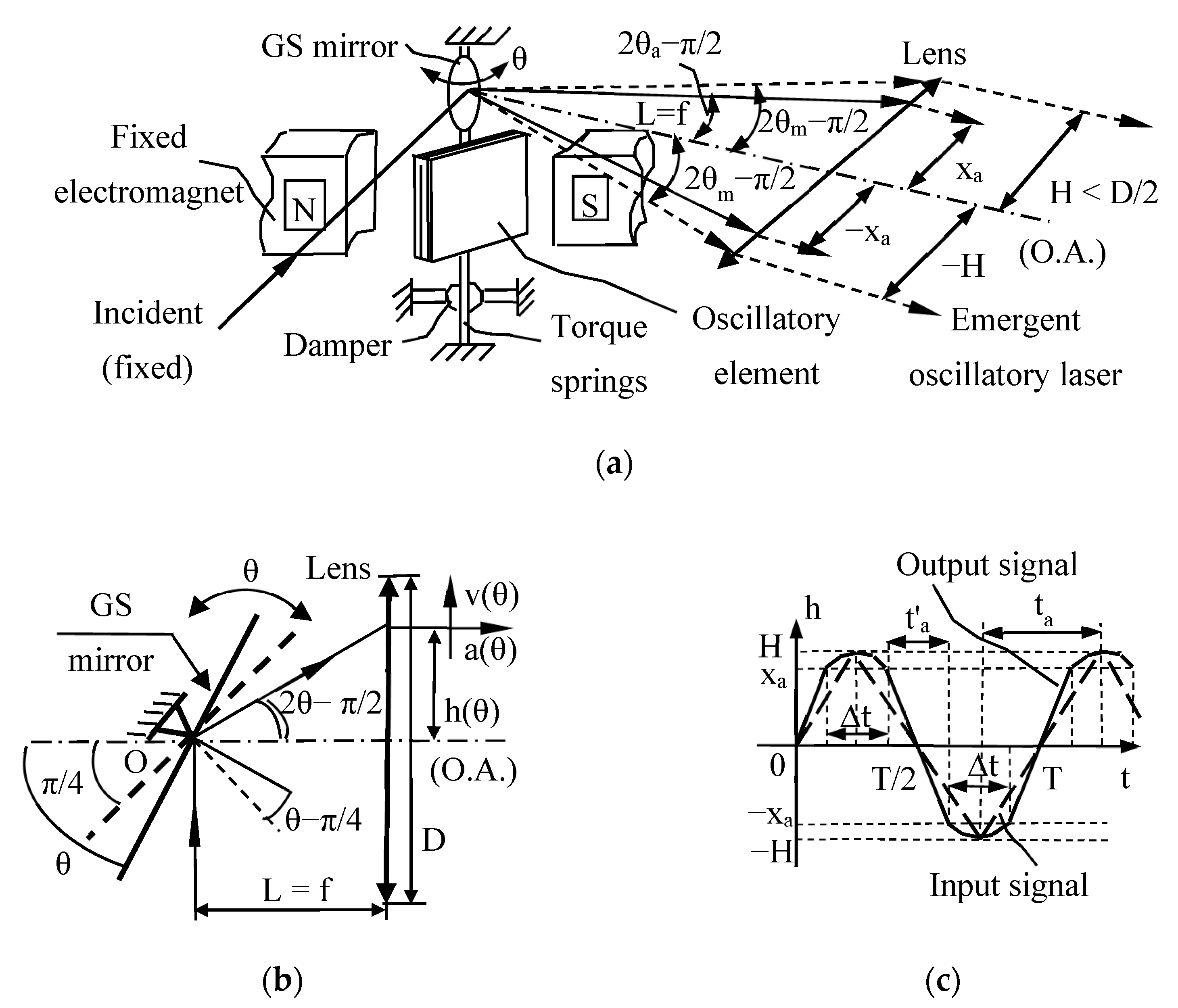
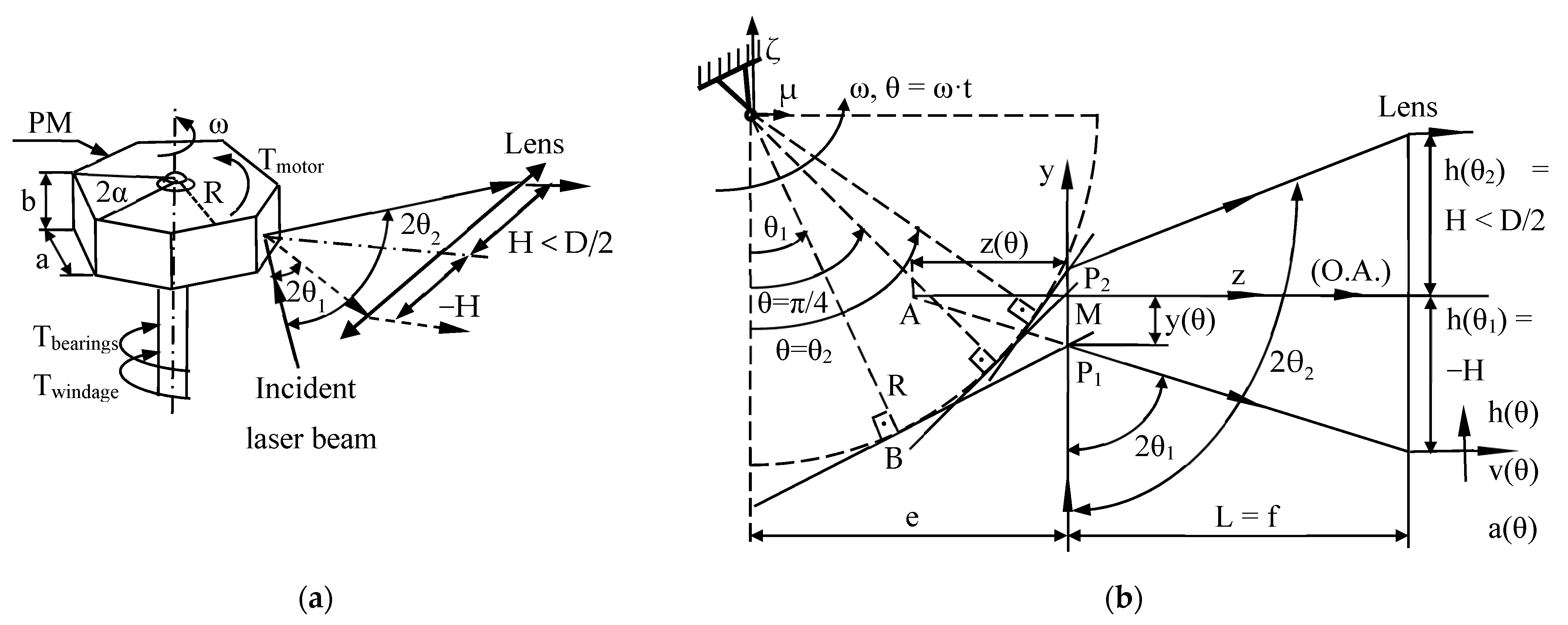
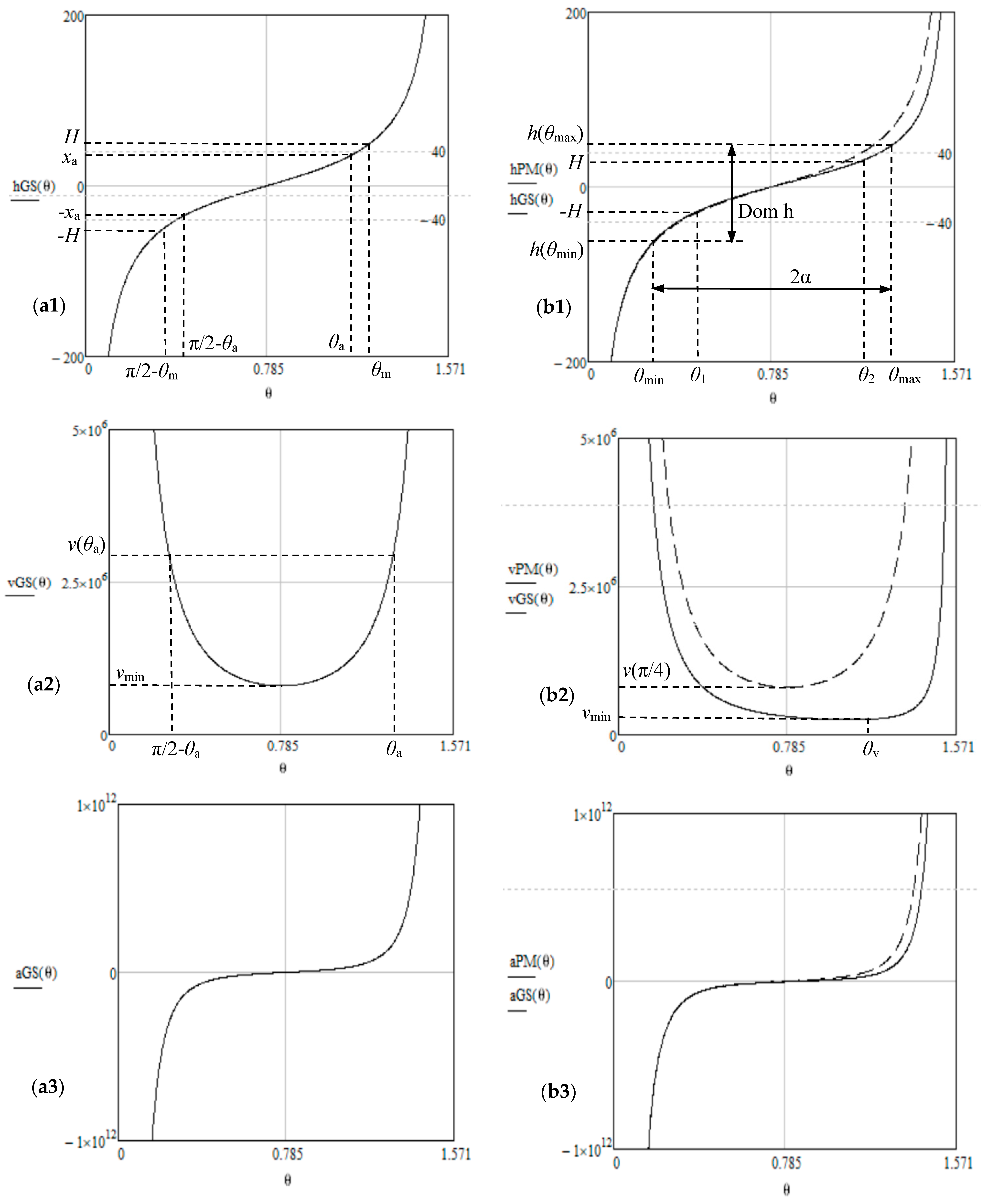
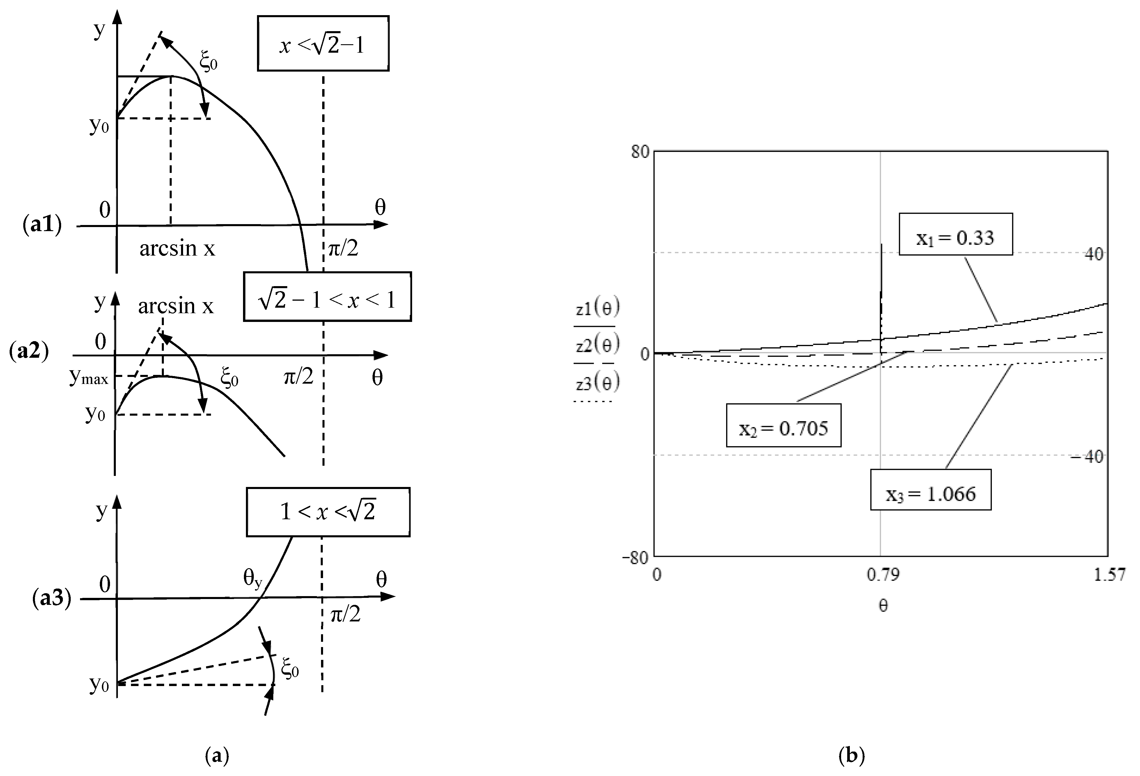
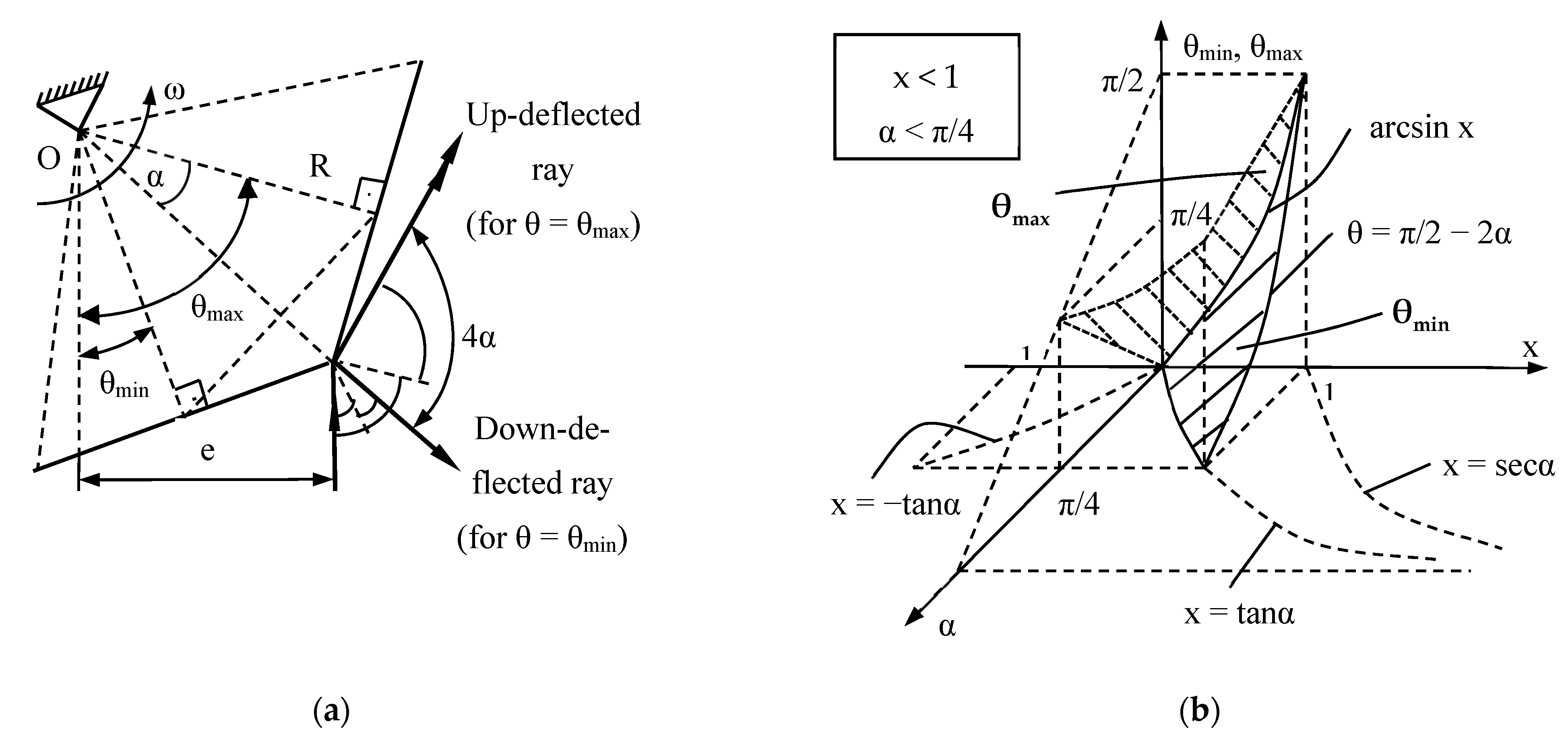
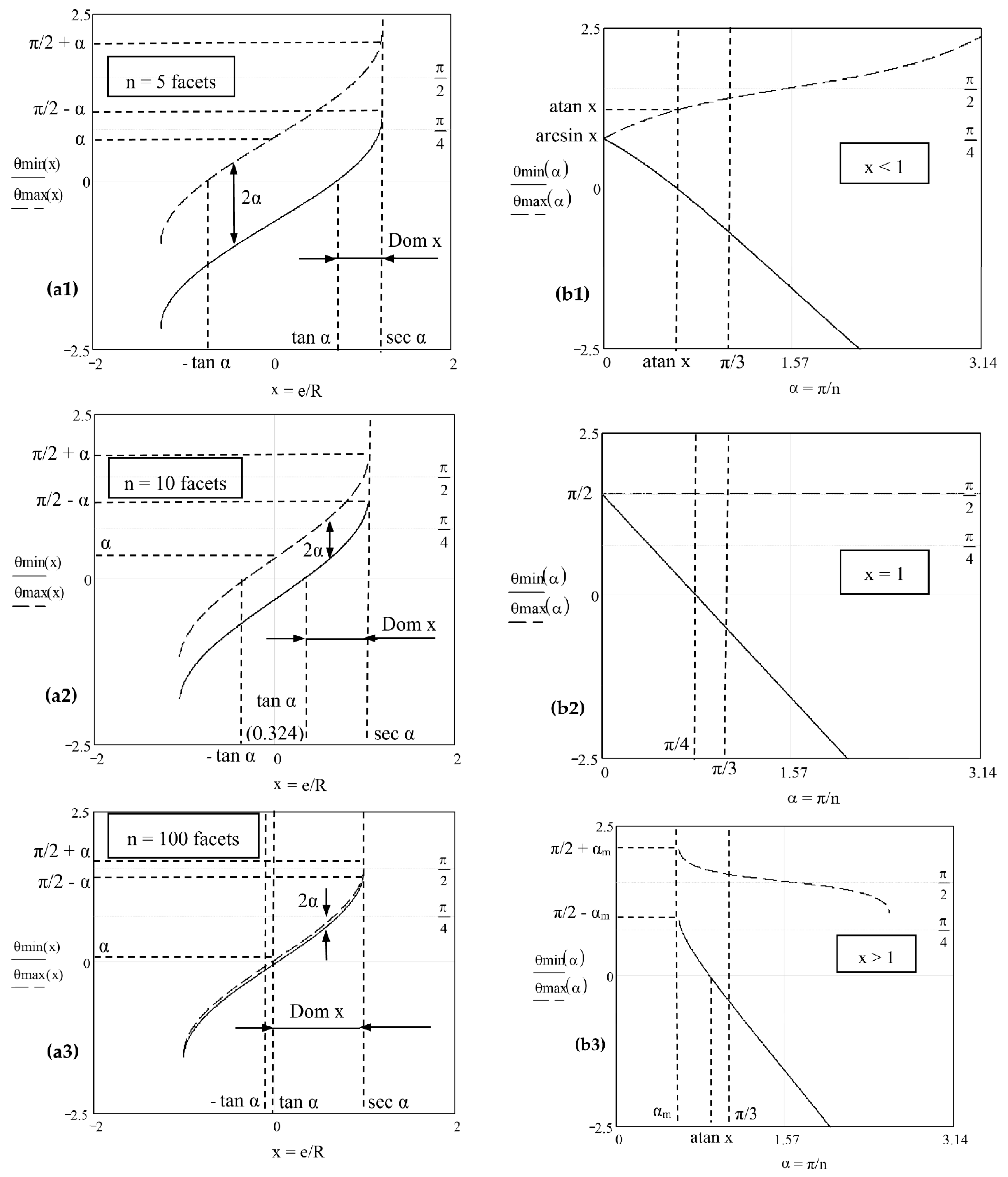
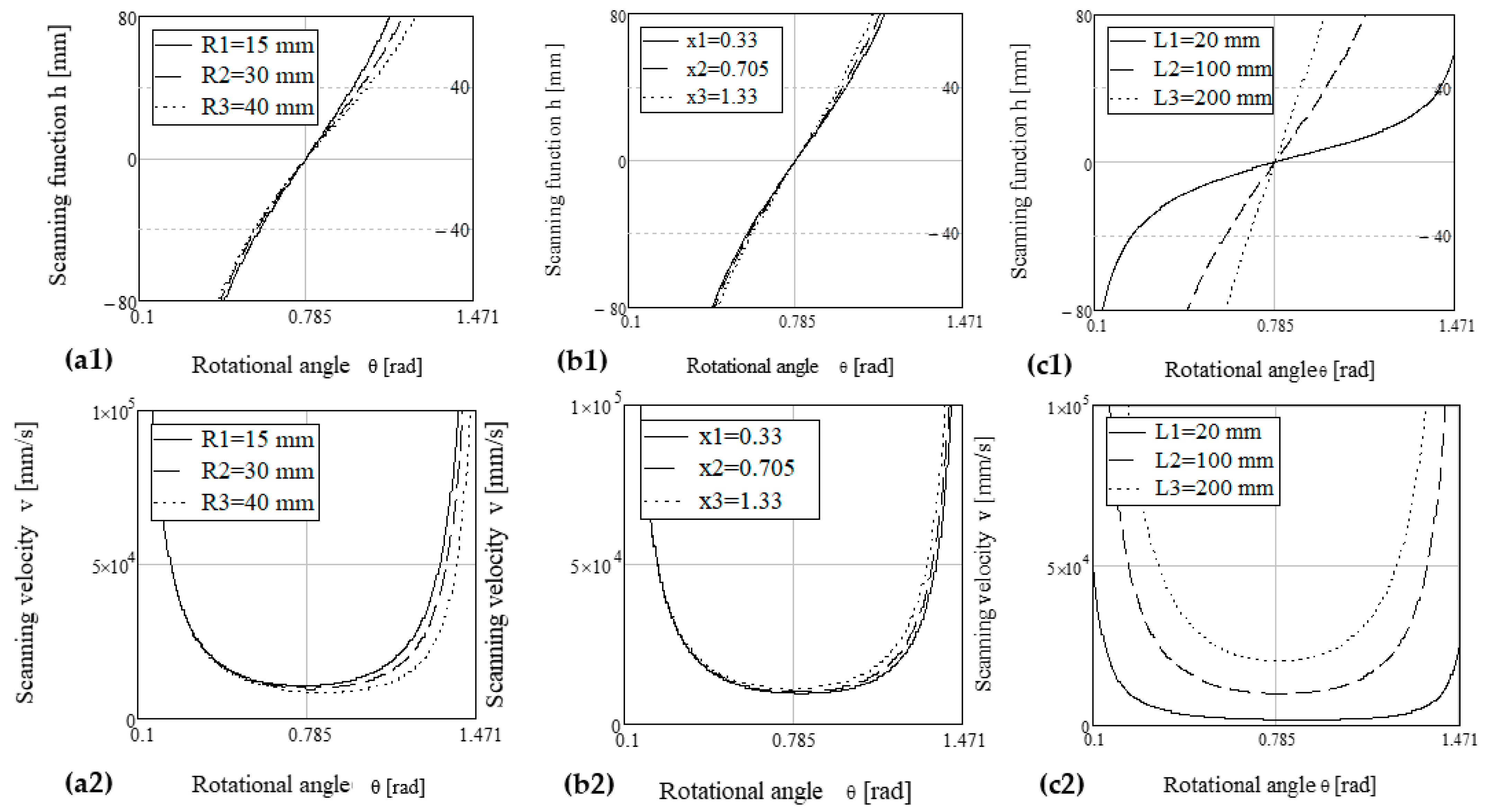
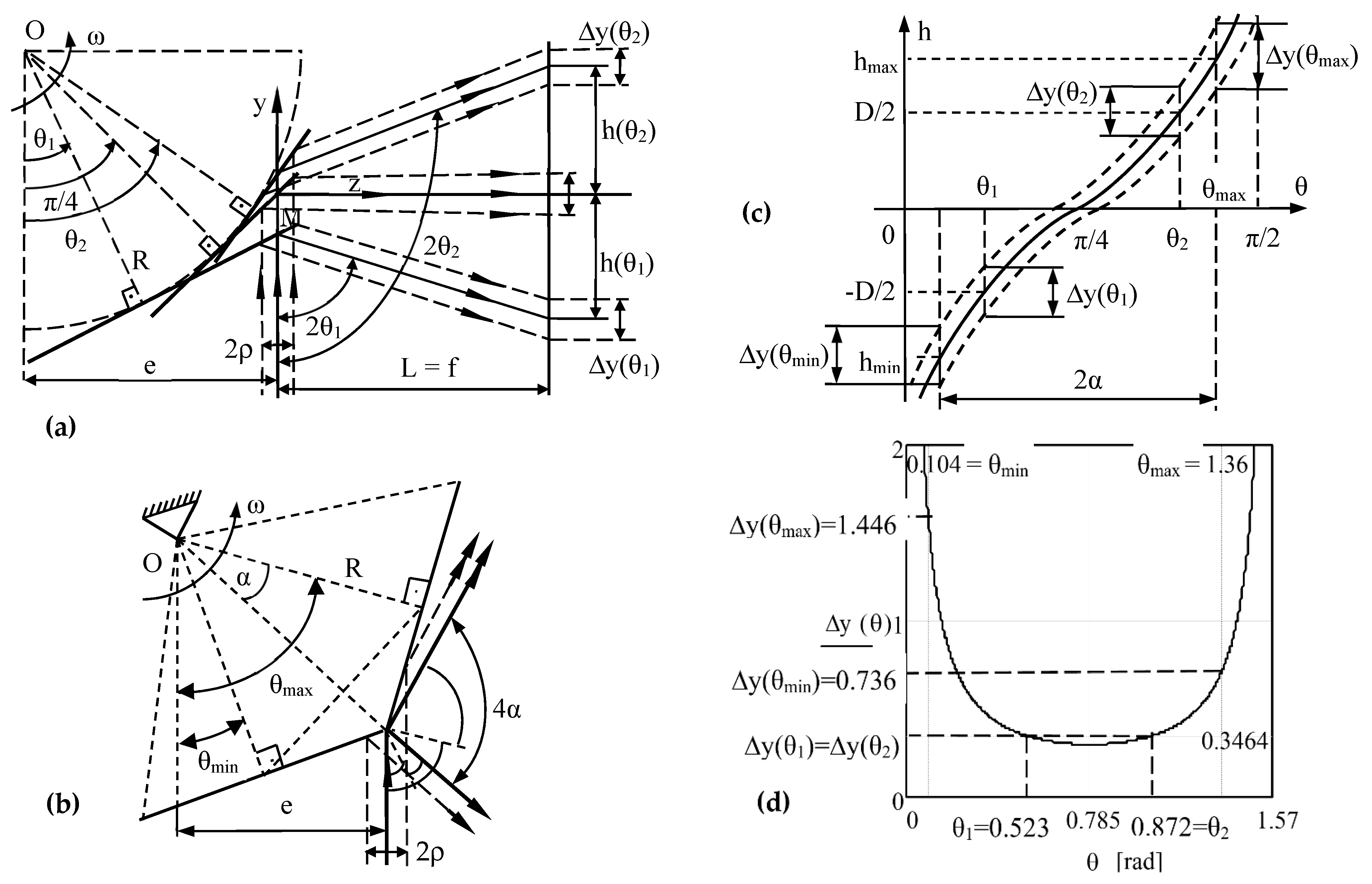
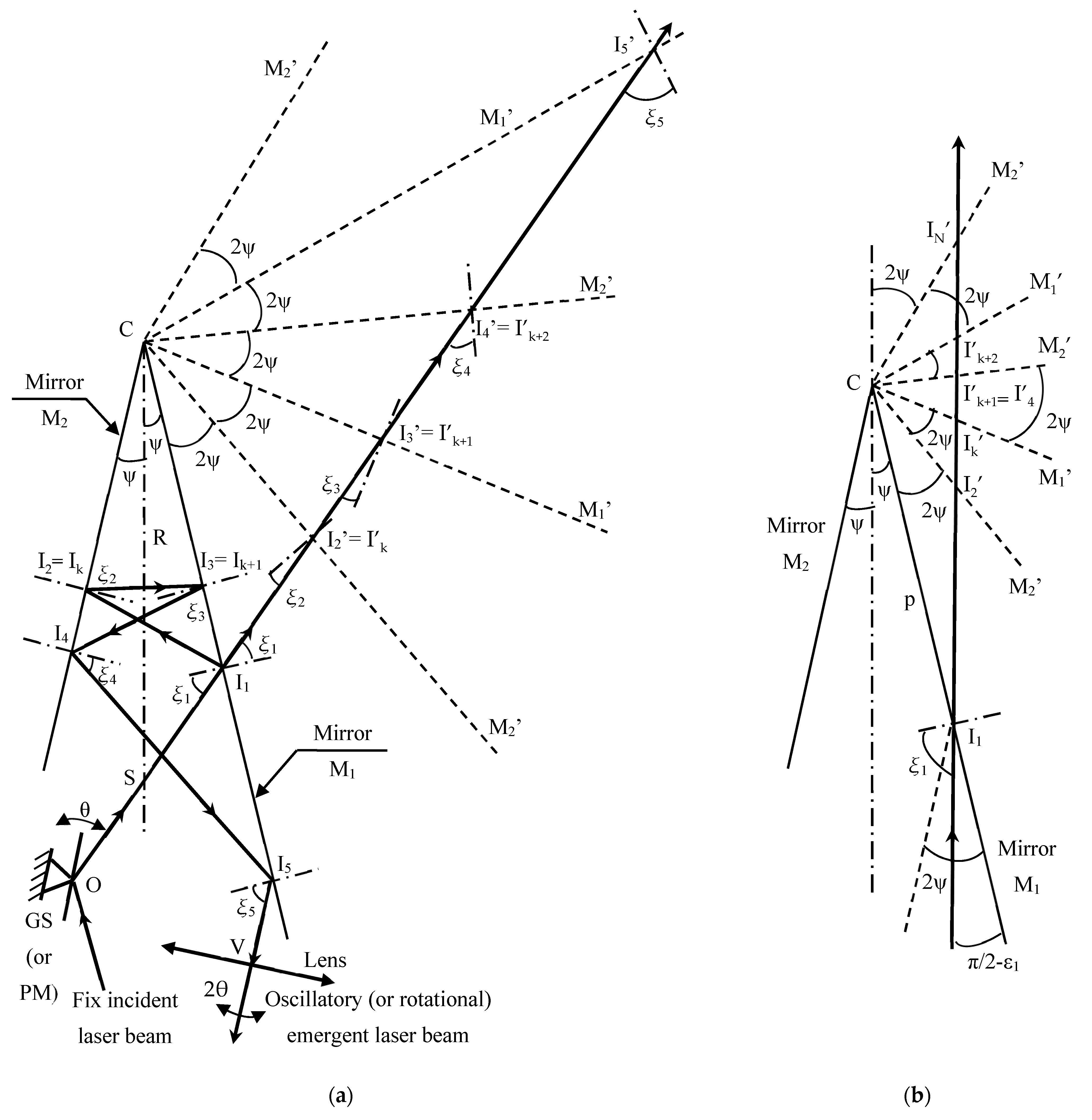
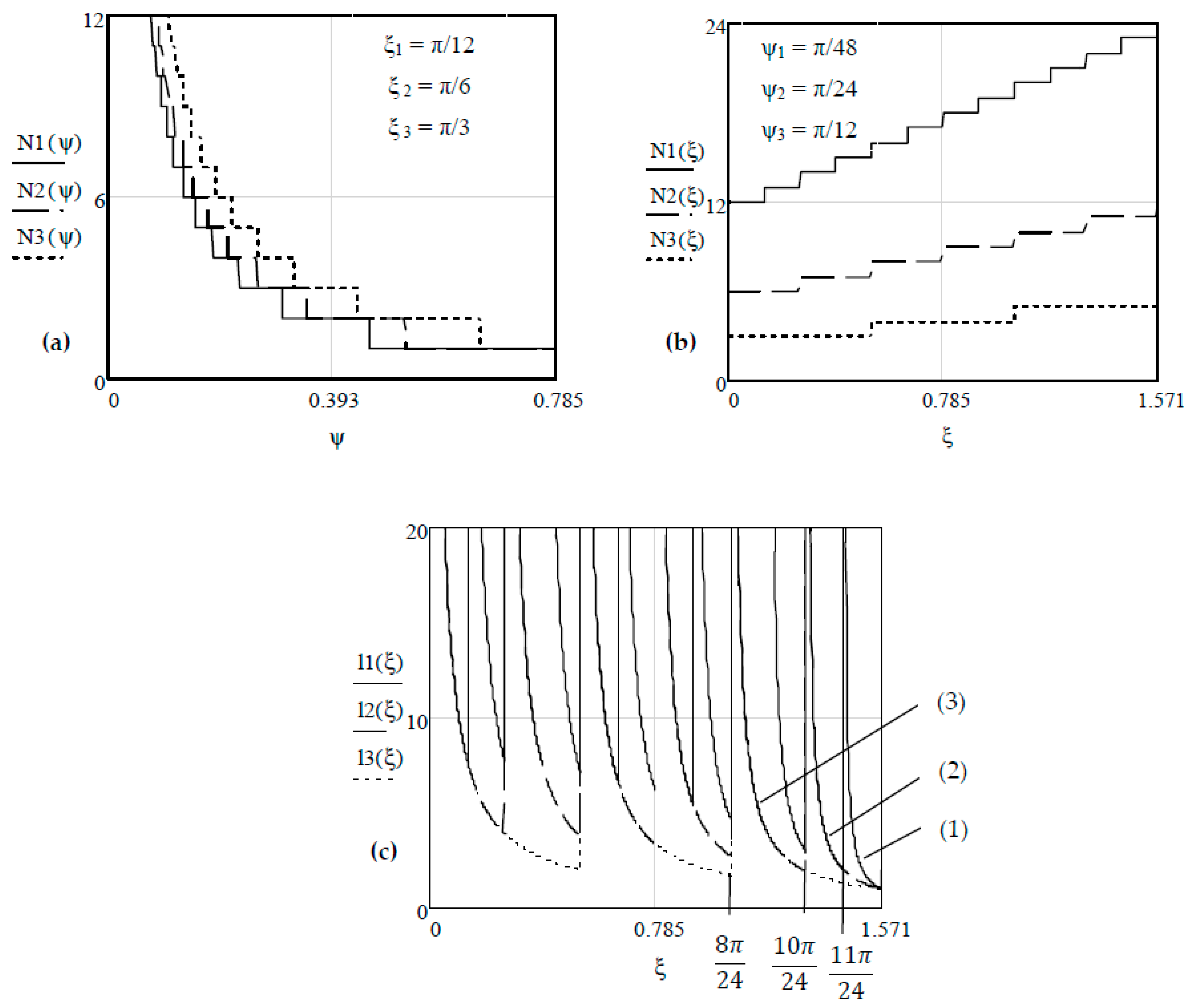
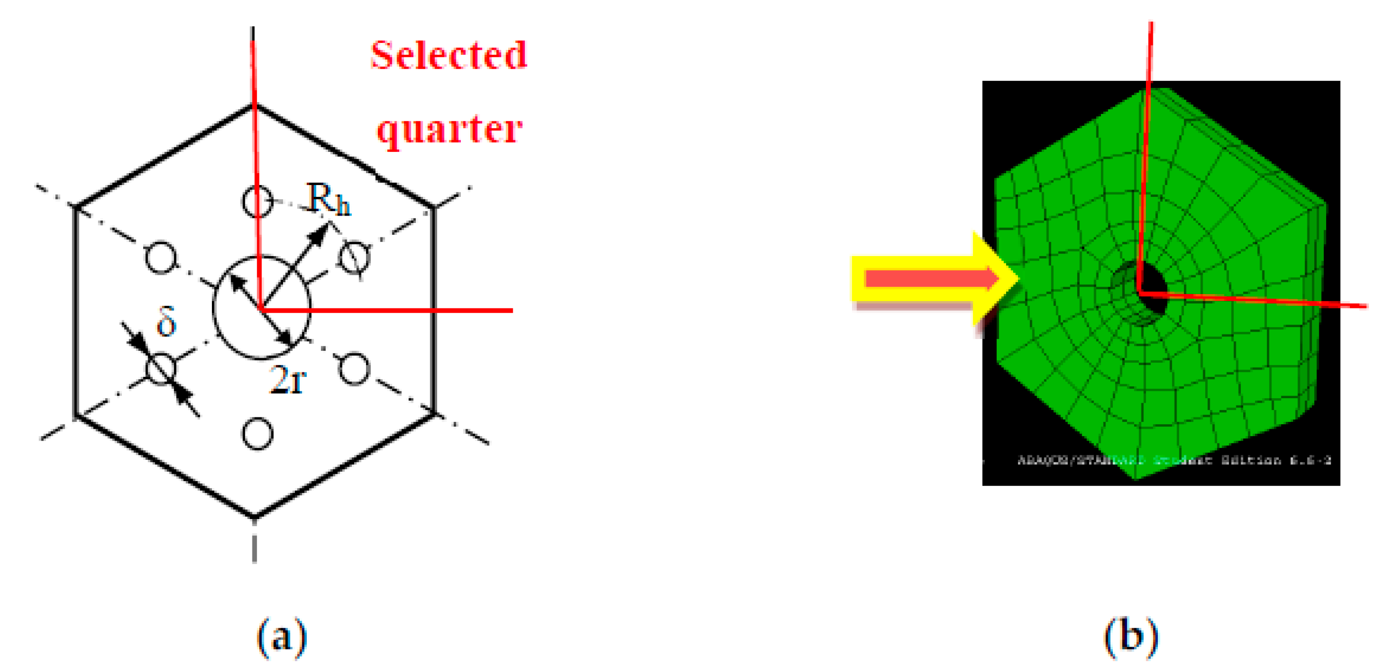
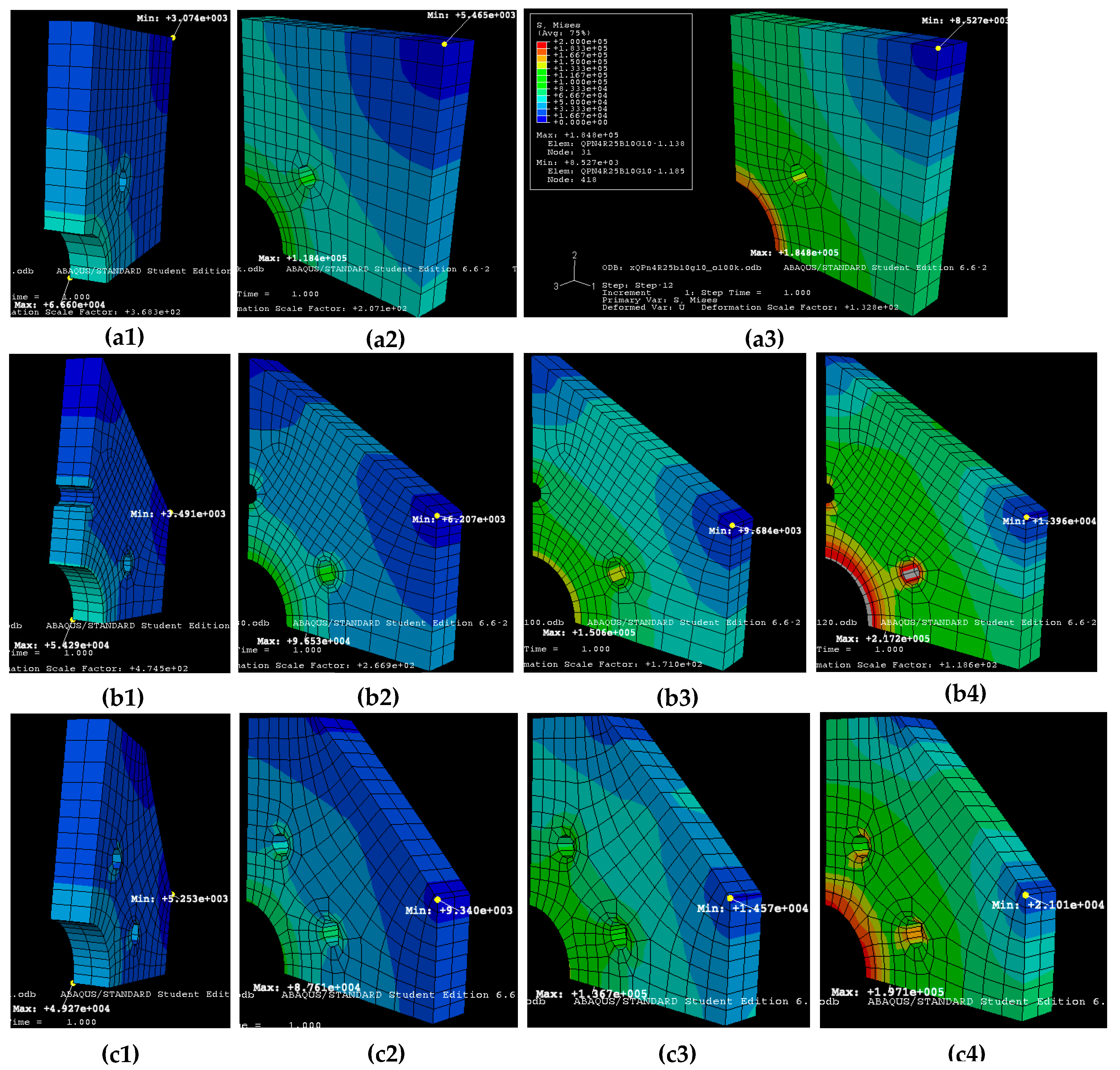
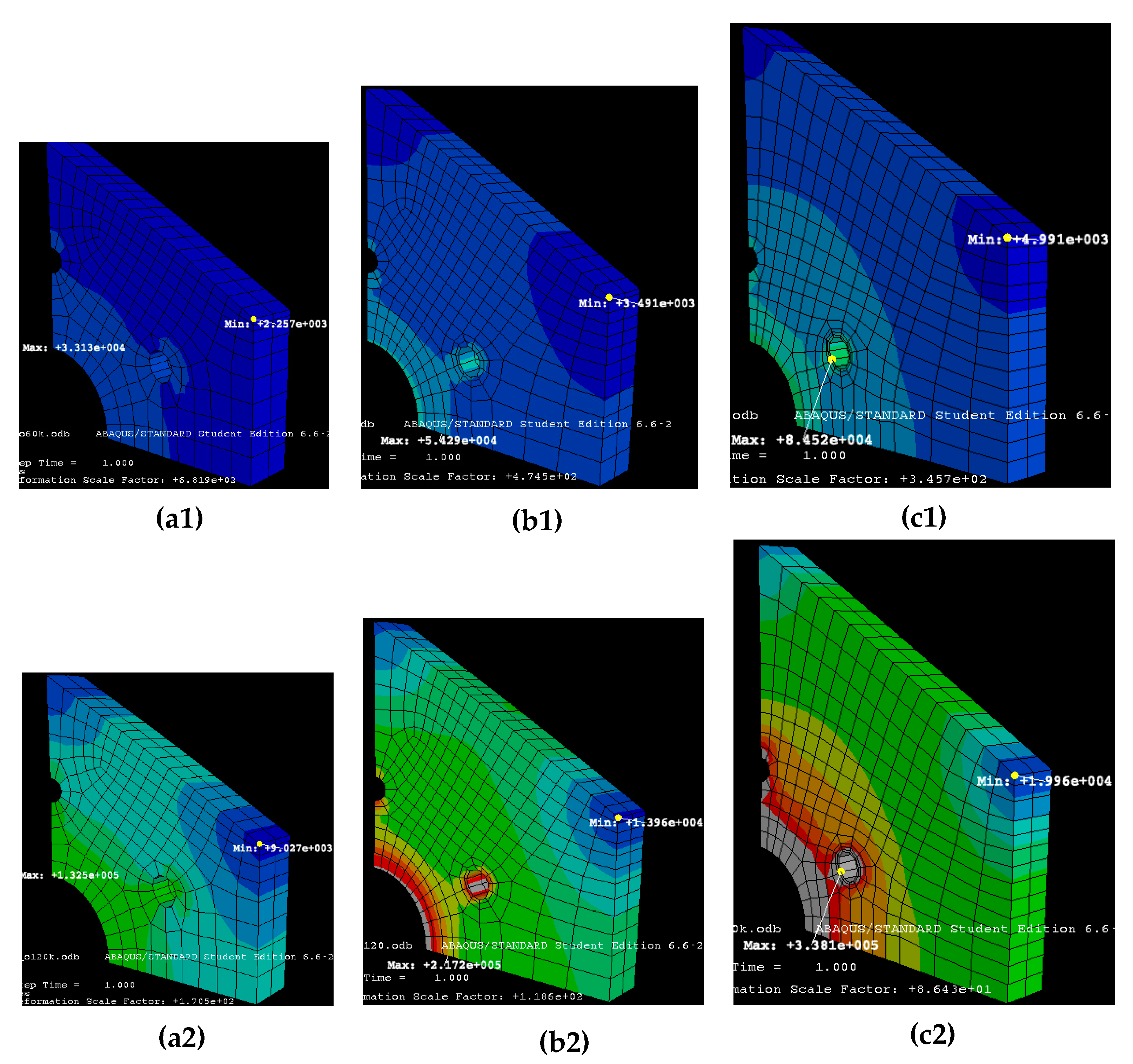
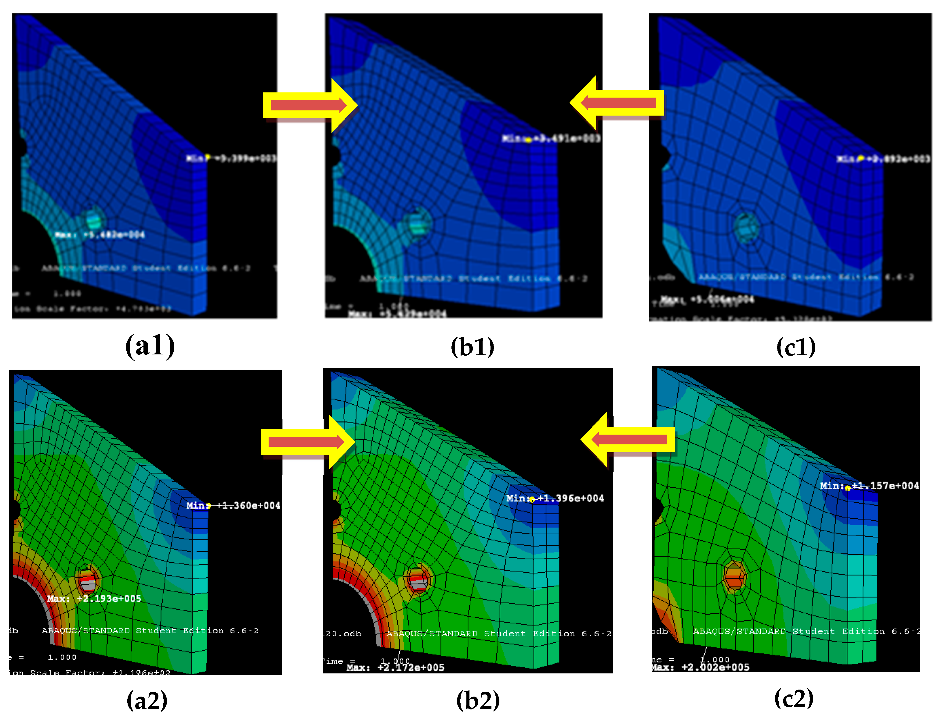
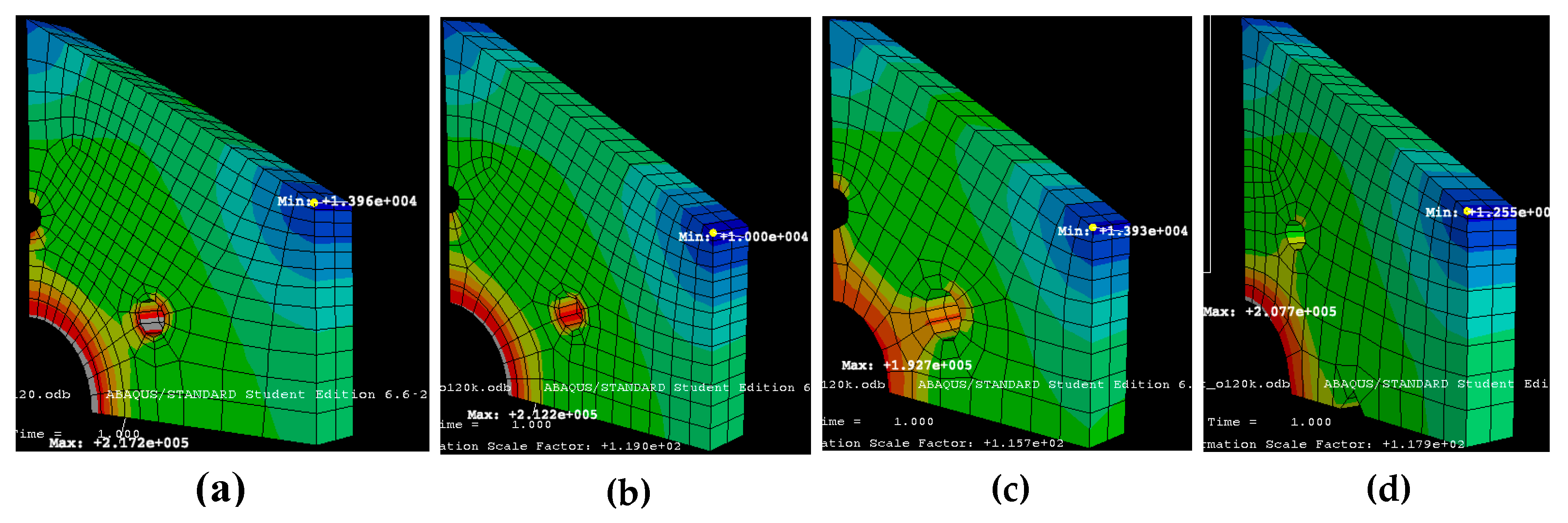
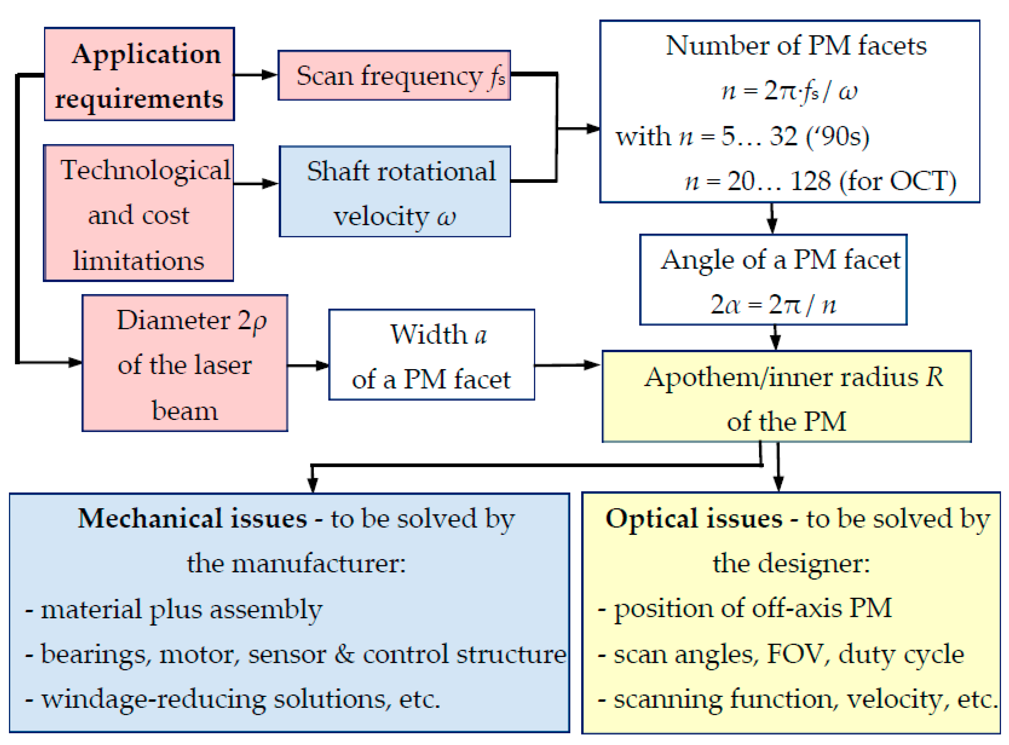
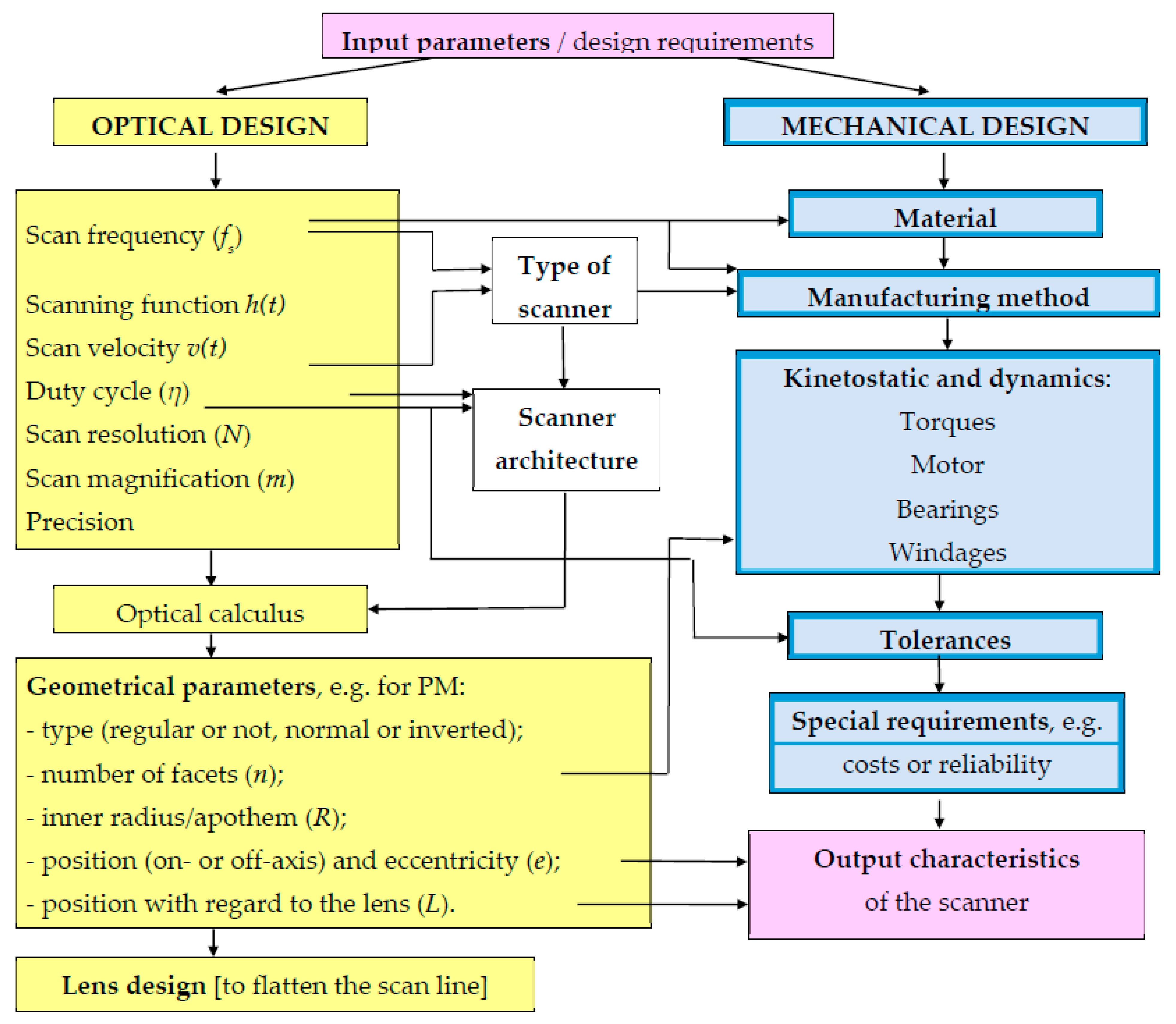
Table 1.
Overview of characteristic functions and parameters of GSs versus PM scanning heads.
| Characteristic Function/Parameter | Galvanometer Scanner (GS) | Polygon Mirror (PM) Scanning Head | |||
|---|---|---|---|---|---|
| Scanning function h(θ) | (1) | (4) | |||
| Scanning velocity | (2) | (5) | |||
| Scanning acceleration | (3) | (6) | |||
| Migration functions | - | Transversal | (7) | ||
| Longitudinal/axial | (8) | ||||
| Scan angles, Figure 1a, Figure 2a and Figure 3 | Extreme | π/2 − θm and θm, where | (9) | (12) | |
| Effective | π/2 − θa and θa, where | (10) | θ1 and θ2, , with H < D/2 | (13) | |
| Field of View (FOV) | Angular | (11) | (14) | ||
| Linear/ Scanning domain | (15) | , where x = e/R | (16) | ||
| Duty cycle, Figure 1a,c and Figure 2a | Theoretical (of the input) | (17) | (19) | ||
| Effective (of the output) | (18) | ||||
Publisher’s Note: MDPI stays neutral with regard to jurisdictional claims in published maps and institutional affiliations. |
© 2022 by the authors. Licensee MDPI, Basel, Switzerland. This article is an open access article distributed under the terms and conditions of the Creative Commons Attribution (CC BY) license (https://creativecommons.org/licenses/by/4.0/).
Share and Cite
MDPI and ACS Style
Duma, V.-F.; Duma, M.-A. Optomechanical Analysis and Design of Polygon Mirror-Based Laser Scanners. Appl. Sci. 2022, 12, 5592. https://0-doi-org.brum.beds.ac.uk/10.3390/app12115592
AMA Style
Duma V-F, Duma M-A. Optomechanical Analysis and Design of Polygon Mirror-Based Laser Scanners. Applied Sciences. 2022; 12(11):5592. https://0-doi-org.brum.beds.ac.uk/10.3390/app12115592
Chicago/Turabian StyleDuma, Virgil-Florin, and Maria-Alexandra Duma. 2022. "Optomechanical Analysis and Design of Polygon Mirror-Based Laser Scanners" Applied Sciences 12, no. 11: 5592. https://0-doi-org.brum.beds.ac.uk/10.3390/app12115592
Note that from the first issue of 2016, this journal uses article numbers instead of page numbers. See further details here.