
Relation of EDL Forces between Clay Particles Calculated by Different Methods


1
State Key Laboratory for Geomechanics and Deep Underground Engineering, China University of Mining and Technology, Xuzhou 221116, China
2
School of Mechanics & Civil Engineering, China University of Mining and Technology, Xuzhou 221116, China
*
Author to whom correspondence should be addressed.
Appl. Sci. 2022, 12(11), 5591; https://0-doi-org.brum.beds.ac.uk/10.3390/app12115591
Submission received: 12 April 2022
/
Revised: 24 May 2022
/
Accepted: 27 May 2022
/
Published: 31 May 2022
(This article belongs to the Special Issue Study on Genesis and Deposition of Clay Minerals)
Abstract
:Calculation of the electrostatic double layer force (EDL force) between clay particles is relevant as it is closely related to important macroscopic mechanical behaviors of clays. The popular method to calculate the EDL force is to integrate the electric potential and Maxwell stress along the boundary enclosing a simply connected domain within which a clay particle resides. The EDL force has also been calculated by the integration of the electrostatic force density over the preceding domain. However, the subtle relation of the EDL forces calculated by the different existing methods has not yet been investigated. By means of theoretical analysis and finite element simulation, it was shown that the force calculated by the integration of Maxwell stress along the complete boundary enclosing a multiply connected domain in which the clay particle is excluded, and that along the partial boundary enclosing the preceding simply connected domain represents the electrical attractive force and osmotic repulsive force, respectively, while the integration of the potential along both the same complete and partial boundary denotes the osmotic force. Numerical results showed that the calculated EDL force deviates from its actual value significantly with the decrease in distance between the chosen integral boundary and particle surface, and the deviation varies with surface potential and angle between particles. Moreover, the recommended minimum distance was proposed to be 10 times the thickness of the particle based on the present simulation results.
1. Introduction
An electrical double layer (EDL) consisting of negative charges on the clay particle surface and the surrounding electrolyte ions in the electric fluid exists widely within natural materials including clay minerals in a watery environment [1,2]. The electrostatic interaction between clay particles due to the overlapping EDLs plays a key role among a variety of engineering contexts, e.g., wellbore stability due to hydration of shale [3], swelling behavior of nuclear waste barrier materials [4], swelling capacity of expansive soil [5], aggregation of coal slurry [6], plasticity of treated clayey soil [7], reduction in soil erosion considering soil organic matter [8], effects of clay swelling/collapse on geological ultrafiltration [9], unfrozen water content in frozen soil [10], fluid–mineral interaction mechanisms underlying enhanced oil recovery [11], efficiency of tailing dewatering [12], and froth flotation of fine coal [13]. To determine the above electrostatic interaction quantitatively, three methods including direct measurement with atomic force microscopy [14,15,16] or surface forces apparatus [17], theoretical or numerical analysis based on the classical theory of Derjaguin, Landau, Verwey, and Overbeek (DLVO) [2,10,13,18,19,20,21,22,23,24,25,26,27,28,29,30,31,32,33,34], and molecular dynamics (MD) simulations [4,5,9,31,35] have often been used in previous studies. Although some deviations from DLVO theory have been revealed by direct measurements and MD simulations [14,15,16,17,35,36,37], e.g., ion–ion correlations (short-range hydration interactions and ion polarization are neglected), DLVO theory is still very reliable under most circumstances [17]. According to this theory, the electrostatic interaction between clay particles is the sum of the van der Waals force and EDL force [2,33,34]. Further, the EDL force is the sum of excess osmotic pressure (it was named the electrical double-layer force in [34], whereas osmotic pressure is used throughout this study to avoid possible confusion) and Maxwell’s stress [23,29,30,31,33]. The osmotic pressure felt by a clay particle is exerted by the electrolyte ions in the EDL, and Maxwell’s stress is the coulomb interaction between charges on the clay particle surface and the counter ions within the EDL [33]. Both of them can be estimated by the electric potential field described by the Poisson–Boltzmann equation.
Although the shape of particles in natural materials including clay minerals may be complex, the material is usually simplified into two parallel infinite plates [8] or ideal spheres [13] based on which the EDL force can be calculated analytically. Scholars from geotechnical engineering have shown that many important mechanical properties of clay such as plasticity [38], compressibility [18,19,20], swelling [22,23,24], and shear strength [25,26] are directly related to the EDL force between clay particles as well as the fabric, i.e., particle arrangement. A reasonable calculation of the EDL force is essential to the deep understanding of the mechanical behavior of clay [25,38]. Early such studies in geotechnical engineering also utilized a simplified particle configuration to represent the actual clay particles system, e.g., Bolt calculated analytically the inter-particle repulsive force based on a model that includes two infinite parallel separate charged plates and indicated that the experimental compressibility of pure clay can be predicted quantitatively well [18].
To investigate the macro-mesoscopic links in mechanical behaviors of soils taking the particle arrangement into account explicitly, the discrete element method (DEM) has been developed into a powerful tool as it was introduced into the field of geotechnical engineering four decades ago [39]. DEM research on clay has made considerable progress in recent years [20,21,22,24,26,27]. A reasonable calculation of the EDL force between clay particles considering the characteristics of finite length and nonparallel arrangement of particles in an actual clay-electrolyte system is necessary for DEM simulations of clay.
Anandarajah and Lu proposed a numerical model to calculate the repulsive force between two inclined charged plate particles with finite length, which are symmetric about a mid-plane in a dielectric medium [28]. This model was frequently used in later DEM simulations of clays [20,21,22,24,27]. However, Maxwell’s stress was not considered explicitly in their model. Recently, the EDL force between two parallel three-dimensional colloidal plates with finite size was calculated numerically [34].
Usually, the calculations of the forces corresponding to osmotic pressure and Maxwell’s stress, which are denoted by osmotic force and electrical force, respectively, are performed by integrations over an arbitrary enclosing boundary [23,32,33] around a charged particle without discussing the possible influence of the location of the enclosing boundary. It has also been shown that the force calculated by the integration of the electrostatic force density over the proper domain [28] is the same as the integration of the potential along the boundary enclosing a simply connected domain, and is in fact the osmotic force. However, to the authors’ knowledge, the subtle relation of the forces calculated by the different existing methods has not yet been investigated. The aim of this paper is to investigate such a relation systematically, which is necessary for correct calculation of the EDL force and thus important for understanding the macroscopic behavior of natural materials involving considerable clay particles.
The remainder of this paper is organized as follows. In Section 2, the calculation methods of EDL forces between charged clay particles in the literature are summarized briefly, and then the relation between the EDL forces calculated by different methods is analyzed. In Section 3, the revealed relations are validated and illustrated by numerical simulations. In Section 4, the conclusions of the present study are drawn.
2. Analysis on the Previous Calculation Methods of EDL Force between Clay Particles
2.1. Previous Methods
As shown in Figure 1, the total EDL force felt by charged clay particles in the electrolyte solution results from two parts: osmotic repulsive stress and electrical (Maxwell) attractive stress.
The total EDL force can be calculated by [33]:
where is the dimensionless potential, Γ is an arbitrary boundary enclosing a simply connected domain within which the clay particle exists, and nj is the direction cosine of the outward normal of this boundary. On the right hand side of the above equation, the item in the first parentheses represents the contribution of osmotic repulsive stresses, while that in the second parentheses denotes the contribution of Maxwell attractive stresses. It has been shown that the calculated total EDL force is independent of the position and size of the enclosed boundary Γ as long as the boundary encloses either one of the two interacting charged clay particle [23,31,33].
In fact, the first integration on the RHS of Equation (1) can also be calculated by integrating the electrostatic force density over the domain that the above boundary Γ is enclosing as [29,32]:
Similarly, using the well-known divergence theorem, the second integration on the RHS of Equation (1) can be rewritten as:
in which the integrand is the dimensionless gradient of the Maxwell stress tensor. As this gradient is the same as the electrostatic force density [29], it can be easily shown that is the same as as long as they have the same integral domain .
2.2. Analysis
In the literature, the boundary Γ in Equation (1) is often chosen to enclose a simply connected domain including one particle, as shown in Figure 1 [23,28,29,31,33]. As there exists an equivalence between Equations (3) and (5), it seems that the total EDL force based on Equation (1) will always be zero. This is obviously wrong while the reason has not yet been investigated [25,29,30,33].
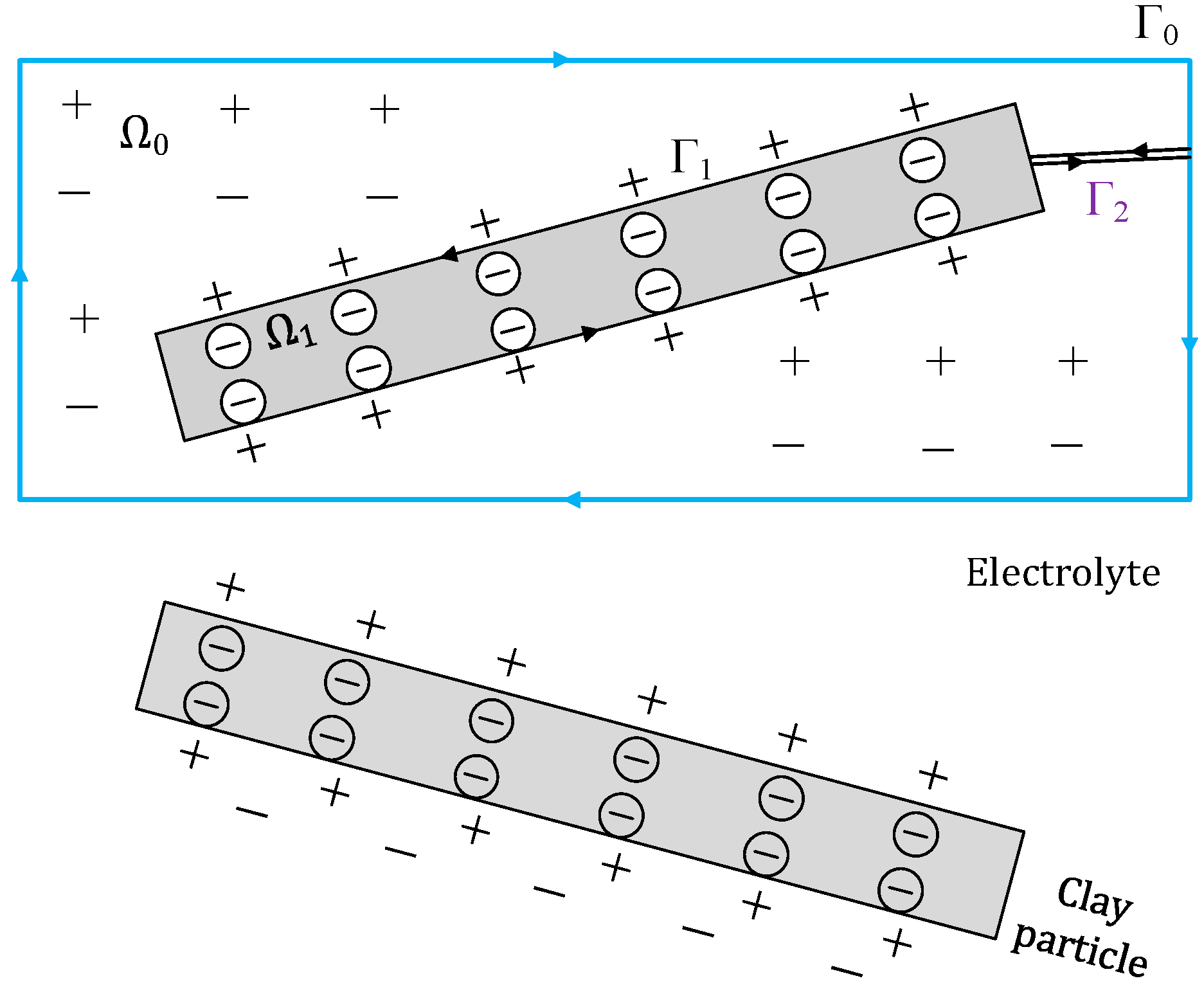
An arbitrary complete enclosing boundary has three parts Γ0, Γ1, and Γ2, as shown in Figure 2, which was adopted by Anandarajah and Lu [28], while they used Equation (2) to calculate the osmotic force and thus did not mention the present issue. Accordingly, the integration in Equation (2) can be divided into three parts. The integrals on Γ1 and Γ2 are zero as the potentials on the opposite sides are the same, but the normal has the opposite sign. Therefore, the first integration in Equation (1) over the complete boundary is that over Γ0 that encloses the usual simply connected domain. This has been studied in [28,32].
Similarly, the integration in Equation (4) can also be divided into three parts, that is:
in which . The third item on the RHS of Equation (6) is zero, as there are the same potential gradients but an opposite normal on the opposite sides of boundary , as shown in Figure 2. However, the first and the second item on the RHS of Equation (6) will not be zero in general. It is especially interesting to notice that the left side in Equation (6) is the minus osmotic repulsive force, while the first item on the RHS of Equation (6) is same as the second integration on the RHS of Equation (1) as boundary just encloses the simply connected domain. Comparing Equation (6) with Equation (1), it can be concluded that the second item on the RHS of Equation (6), i.e., the integration of the Maxwell stress exactly on the surface of the clay particle, is in fact the total EDL force between clay particles.
As a summary, both of the forces calculated by integrating the electrostatic force density or the gradient of Maxwell stress over a domain within which one clay particle resides, and the force calculated by the counterpart integration alone of the complete boundary enclosing a multiply connected domain in which the surrounding electrolyte and clay particle are separated, are the osmotic force. The integration of Maxwell stress along the partial boundary enclosing a simply connected domain including one particle represents the contribution of electrical force related to Maxwell stress, while the integration related to electrostatic force density along the same partial boundary denotes the osmotic force. In the following section, a numerical method is adopted to illustrate the above conclusions.
3. Illustration
In order to calculate the above forces, the potential distribution around the clay–electrolyte system, as shown in Figure 2, has to be obtained by solving the following dimensionless Poisson–Boltzmann equation.
A numerical procedure based on the finite element method [40] developed previously by the author is used here [31].
3.1. Simulation Scheme
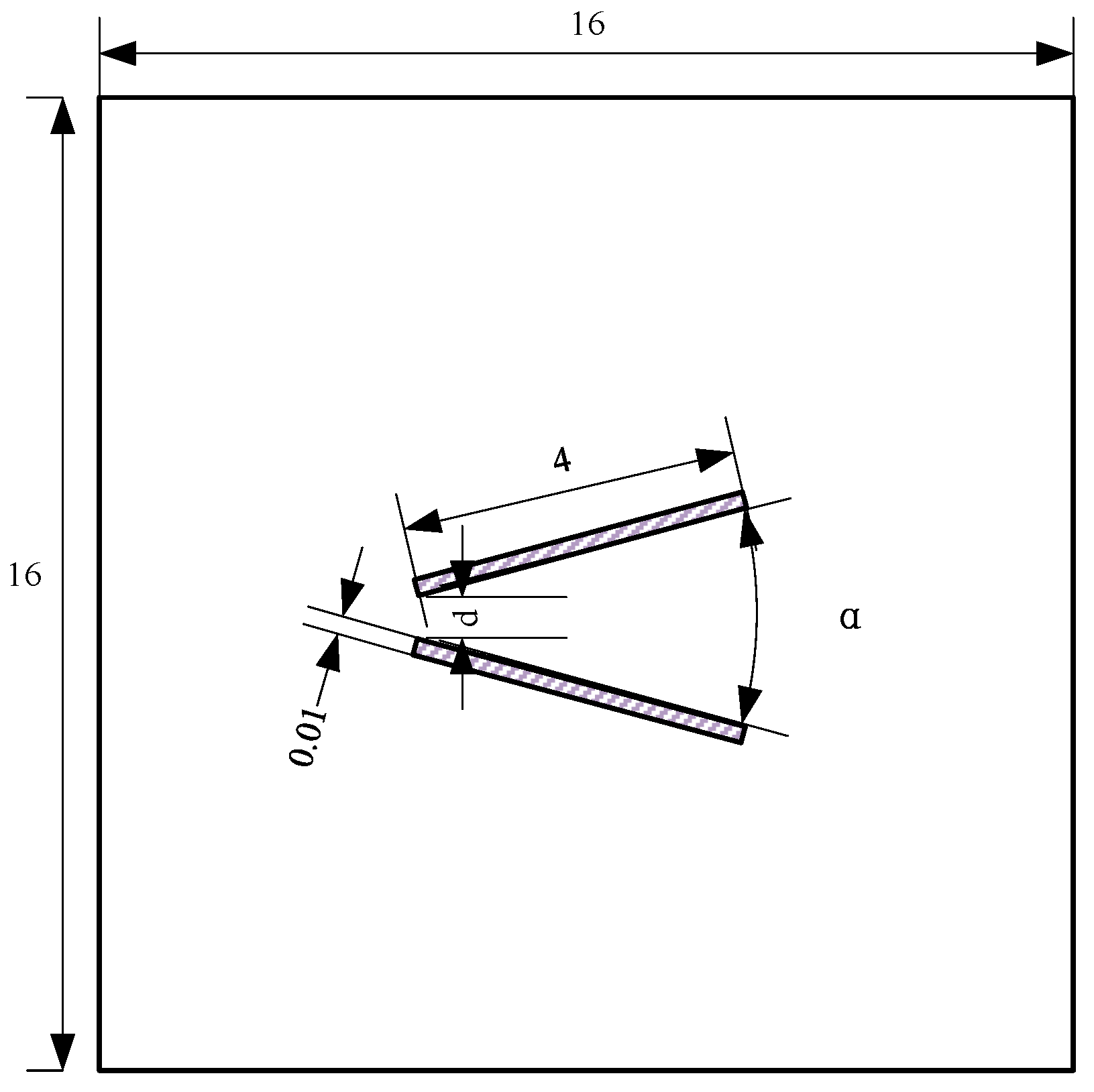
The numerical model consists of two finite inclined charged plates denoting clay particles in an electrolyte solution. The size of the model and the particles and the separation between particles are presented in Figure 3. It should be noted that the size is also dimensionless as all the aforementioned quantities are dimensionless. A constant length of 4 and thickness of 0.01 are chosen to represent a typical clay particle, while the particle surface potential , angle , and minimum distance between two particles d, as shown in Figure 3, are considered as variables as they have a pronounced effect on the calculated repulsion [31]. The designed simulation scheme is summarized in Table 1. Among the simulations, the case of = 60°, d = 1.0, and = 5.0 is taken as the basic case around which the three abovementioned factors change according to the designed simulation scheme.
The potential on the outmost boundary of the model is zero, i.e., this boundary is regarded as infinity. A very fine mesh near the charged plates is adopted to accommodate the high potential gradient around the particle surface. Based on the necessary mesh sensitivity analysis, the final finite element mesh used in the numerical simulation consists of around 700 thousand triangle elements and 350 thousand nodes. The used mesh and calculated potential nephogram are shown in Figure 4.
Once the numerical electric potential field is obtained, various electric forces between clay particles can be determined based on Equations (2)–(5). For each simulation, different integral domains including one particle and some surrounding electrolyte were chosen to calculate the corresponding force. It should be noted that for the case of two symmetric inclined particles, as shown in Figure 3, the repulsive force is along the vertical direction due to the symmetry [28]. Thus, only the vertical forces are presented in the following.
Figure 5 presents the integral domain by a dashed line box. The location and size of the domain can be defined by four distances, xL, xR, yU, and yD shown in this figure. Eight combinations of these four distances were chosen, as shown in Table 2. Case (1) in this table is the largest domain that is in fact the upper half of model, while case (8) represents the smallest domain in which the distance between the outmost boundary of the domain and the particle is only 1% of the thickness of the particle. The rest are somewhere in between.
3.2. Simulation Results
It can be seen that the accuracy of Equation (3) depends on the first-order derivative of the calculated potential over the selected domain, Equation (2) has the higher accuracy that depends on the calculated potential over the corresponding enclosing boundary, Equation (5) has the lowest accuracy that depends on the second derivative of the calculated potential over the selected domain, and the accuracy of Equation (4) is higher than that of Equation (5) but lower than that of Equation (3). To illustrate the effect of the preceding numerical accuracy and the revealed relation, the forces calculated based on Equations (2)–(5) along partial boundary Γ0, and on Equation (1) with the second integration on the RHS being along Γ0, are present from the second column to sixth column.
Due to the fact that the integration in Equation (5) along Γ1 is affected significantly by the high potential gradient, an additional approximate boundary with length and width of 4.001 and 0.011, respectively, was used to replace Γ1 to obtain a more reasonable calculated force. As shown in the last column in Table 3, ‘A’ is the calculated force based on the approximate surface, while ‘E’ is that based on exact Γ1.
3.3. Discussion
Comparing the calculated forces between the second, third, and fourth column in Table 3, which correspond to Equation (2), Equation (3), and Equation (5), respectively, it can be seen that the forces calculated by Equations (2) and (3) are almost the same except for the last case shown of = 60°, = 1.0, and = 10 in Table 3(C2) where a large surface potential and inclination of a clay particle likely lead to a highly nonuniform potential field. The equivalence between the forces calculated by Equations (3) and (5) can only be observed for the case of = 0°, = 1.0, and = 5 with a relatively large integral domain shown in Table 3, and the deviation between them increases with increasing angle and potential and decreasing integral domain. This results from the different accuracy of Equations (2), (3) and (5), as explained in Section 3.2.
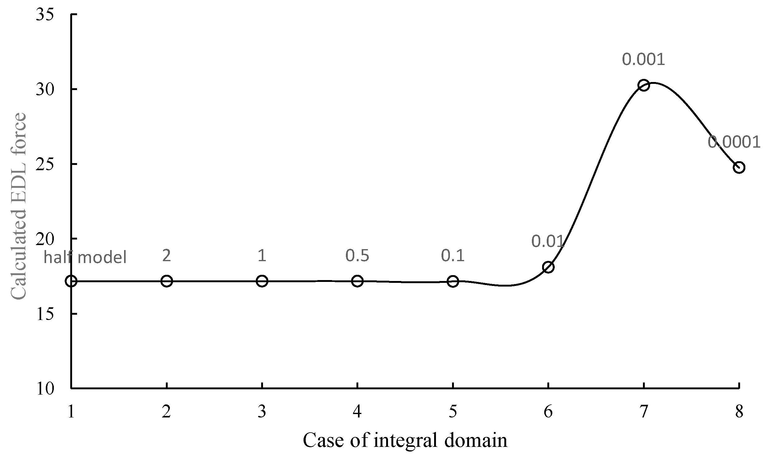
Comparing the forces between the sixth and last column shown in Table 3, it can be observed that the last column, i.e., the integration of Maxwell stress along a boundary approximate to , is almost the same as the total EDL force in the sixth column, which is calculated using Equation (1). Similarly, the deviation between them increases nonlinearly with surface potential, angle, and distance. Therefore, it can be seen that the integration of Maxwell stress just along the surface of the clay particle is indeed the total EDL force between clay particles, while that along the complete boundary enclosing a multiply connected domain is the osmotic repulsive force. For the ideal case of two infinite parallel charged plates, Verwey and Overbeek [1] used Equation (2) choosing a partial enclosing boundary similar to Γ0, as shown in Figure 2, which corresponds to a simply connected domain bounded by the mid-plane and infinity. This method was widely adopted in the later studies [5,10,13,23,28,29,31,33,34]. On the contrary, Derjaguin and Landau [41] used Equation (4) choosing an enclosing boundary identical to Γ1, as shown in Figure 2, which is just the surface of the enclosed particle. For the ideal case of infinite parallel particles, analytical solutions based on the above two methods are the same [33]. For the actual case of particles with finite size, the contribution of Maxwell’s stress was usually taken into account numerically by Equation (4) choosing the enclosing boundary similar to Γ0 [8,17,23] without considering the possible adverse effect of numerical accuracy. However, as illustrated in Table 3, the calculated contribution of Maxwell’s stress is prone to be affected by the selection of an integral boundary. As an example, the calculated EDL forces for the case of α = 60°, d = 1.0, and ϕ0 = 10 with different integral boundaries listed in Table 2 are shown in Figure 6 in which the characteristic distances between the integral boundary and particle surface presented in Table 3 are also shown. It can be seen that the calculated EDL force deviates remarkably when the chosen integral boundary is close enough to the particle.
Another example of the case of α = 120°, d = 1.0, and ϕ0 = 5 is shown in Figure 7, and it can be seen that the calculated EDL force that is actually repulsive can become attractive due to the computation error when the chosen integral boundary is close enough to the particle surface. Therefore, it will likely lead to a misunderstanding of the aggregation or dispersion of relevant soils [6,8,13] if the above-mentioned relation is not taken into account reasonably.
An interesting observation that can be obtained by checking all the sixth columns in Table 3 is that the distance between the integral boundary and the particle should be larger than 0.1, i.e., 10 times the thickness of the particle of 0.01; otherwise, the numerical error in the calculated EDL force is likely to be out of control. This means that the enclosed boundary Γ as shown in Equation (1) should be chosen with caution, although the calculated EDL force is independent of its position and size theoretically [8,17,33]. This would be the case when the above interaction between dense clay particles needs to be evaluated, as with the DEM simulation of the clay sample [6,7,13].
4. Conclusions
The total repulsive forces between two charged clay particles consist of two parts: osmotic repulsive force and electrical/Maxwell attractive force. They are usually calculated by the integrations of potential and Maxwell stress along a partial boundary enclosing a simply connected domain including one clay particle in the literature. Based on the analysis and numerical validation, the following conclusions are obtained:
- (1)
- The integration of electrostatic force density, i.e., Maxwell stress gradient over a domain including one particle and surrounding electrolyte, or the integration of the potential and Maxwell stress along the complete boundary enclosing a multiply connected domain in which the surrounding electrolyte and the clay particle are separated, are the same osmotic repulsive force. However, the divergence between them will be inevitably observed in the numerical solution, and it increases nonlinearly with the surface potential, angle, and distance between clay particles.
- (2)
- The integration of Maxwell stress along the partial boundary enclosing a simply connected domain within which one particle exists represents the contribution of electrical (Maxwell) attractive stress. However, the integration of the potential along the same partial boundary denotes the osmotic repulsive force.
- (3)
- The integration of Maxwell stress exactly on the surface of the clay particle is in fact the total EDL force between clay particles. However, it is impractical to calculate a reasonable force by means of numerical method.
- (4)
- Although the calculated total repulsive stress is independent of its position and size theoretically, it is recommended that the distance between the integral box and the particle should be at least 10 times the thickness of the particle, based on the present numerical simulations.
Funding
This research was funded by Fundamental Research Funds for the Central Universities (Grant number, 2020ZDPYMS18).
Institutional Review Board Statement
Not applicable.
Informed Consent Statement
Not applicable.
Conflicts of Interest
The authors declare no conflict of interest.
References
- Verwey, E.J.W.; Overbeek, J.T.G. Theory of the Stability of Lyophobic Colloids; Elsevier: Amsterdam, The Netherlands, 1948. [Google Scholar]
- Van Olphen, H. An Introduction to Clay Colloid Chemistry: For Clay Technologists, Geologists, and Soil Scientists; Wiley: New York, NY, USA, 1977. [Google Scholar]
- Lv, K.; Liu, J.; Jin, J.; Sun, J.; Huang, X.; Liu, J.; Guo, X.; Hou, Q.; Zhao, J.; Liu, K.; et al. Synthesis of a novel cationic hydrophobic shale inhibitor with preferable wellbore stability. Colloids Surf. A Physicochem. Eng. Asp. 2022, 637, 128274. [Google Scholar] [CrossRef]
- Yang, Y.; Qiao, R.; Wang, Y.; Sun, S. Swelling pressure of montmorillonite with multiple water layers at elevated temperatures and water pressures: A molecular dynamics study. Appl. Clay Sci. 2021, 201, 105924. [Google Scholar] [CrossRef]
- Du, J.; Zhou, A.; Lin, X.; Bu, Y.; Kodikara, J. Prediction of swelling pressure of expansive soil using an improved molecular dynamics approach combining diffuse double layer theory. Appl. Clay Sci. 2021, 203, 105998. [Google Scholar] [CrossRef]
- Li, H.; Chen, J.; Peng, C.; Min, F.; Song, S. Salt coagulation or flocculation? In situ zeta potential study on ion correlation and slime coating with the presence of clay: A case of coal slurry aggregation. Environ. Res. 2020, 189, 109875. [Google Scholar] [CrossRef]
- Vitale, E.; Deneele, D.; Russo, G. Microstructural investigations on plasticity of lime-treated soil. Minerals 2020, 10, 386. [Google Scholar] [CrossRef]
- Yu, Z.; Zheng, Y.; Zhang, J.; Zhang, C.; Ma, D.; Chen, L.; Cai, T. Importance of soil interparticle forces and organic matter for aggregate stability in a temperate soil and a subtropical soil. Geoderma 2020, 362, 114088. [Google Scholar]
- Zhou, H.; Chen, M.; Zhu, R.; Lu, X.; Zhu, J.; He, H. Coupling between clay swelling/collapse and cationic partition. Geochim. Cosmochim. Acta 2020, 285, 78–99. [Google Scholar] [CrossRef]
- Jin, X.; Yang, W.; Gao, X.; Zhao, J.-Q.; Li, Z.; Jiang, J. Modeling the unfrozen water content of frozen soil based on the absorption effects of clay surfaces. Water Resour. Res. 2020, 56, e2020WR027482. [Google Scholar] [CrossRef]
- Xie, Q.; Liu, F.; Chen, Y.; Yang, H.; Saeedi, A.; Hossain, M. Effect of electrical double layer and ion exchange on low salinity EOR in a pH controlled system. J. Pet. Sci. Eng. 2019, 174, 418–424. [Google Scholar] [CrossRef]
- Abraham, T.; Lam, N.; Xu, J.; Zhang, D.; Wadhawan, H.; Kim, H.J.; Lee, M.; Thundat, T. Collapse of house-of-cards clay structures and corresponding tailings dewatering induced by alternating electric fields. Dry. Technol. 2019, 37, 1053–1067. [Google Scholar] [CrossRef]
- Yu, Y.; Ma, L.; Xu, H.; Sun, X.; Zhang, Z.; Ye, G. DLVO theoretical analyses between montmorillonite and fine coal under different pH and divalent cations. Powder Technol. 2018, 330, 147–151. [Google Scholar] [CrossRef]
- Scarratt, L.R.J.; Kubiak, K.; Maroni, P.; Trefalt, G.; Borkovec, M. Structural and double layer forces between silica surfaces in suspensions of negatively charged nanoparticles. Langmuir 2020, 36, 14443–14452. [Google Scholar] [CrossRef]
- Stojimirovicć, B.; Vis, M.; Tuinier, R.; Philipse, A.P.; Trefalt, G. Experimental evidence for algebraic double-layer forces. Langmuir 2020, 36, 47–54. [Google Scholar] [CrossRef] [Green Version]
- Feng, B.; Liu, H.; Li, Y.; Liu, X.; Tian, R.; Li, R.; Li, H. AFM measurements of Hofmeister effects on clay mineral particle interaction forces. Appl. Clay Sci. 2020, 186, 105443. [Google Scholar] [CrossRef]
- Smith, A.M.; Borkovec, M.; Trefalt, G. Forces between solid surfaces in aqueous electrolyte solutions. Adv. Colloid Interface Sci. 2020, 275, 102078. [Google Scholar] [CrossRef]
- Bolt, G.H. Physico-chemical analysis of the compressibility of pure clays. Geotechnique 1956, 6, 86–93. [Google Scholar] [CrossRef]
- Bharat, T.V.; Sridharan, A. Prediction of compressibility data for highly plastic clays using diffuse double-layer theory. Clays Clay Miner. 2015, 63, 30–42. [Google Scholar] [CrossRef]
- Bayesteh, H.; Mirghasemi, A.A. Numerical simulation of pore fluid characteristic effect on the volume change behavior of montmorillonite clays. Comput. Geotech. 2013, 48, 146–155. [Google Scholar] [CrossRef]
- Yuan, G.; Xiong, Y. A holistic computational model for prediction of clay suspension structure. Int. J. Sediments Res. 2019, 34, 345–354. [Google Scholar]
- Bayesteh, H.; Hoseini, A. Effect of mechanical and electro-chemical contacts on the particle orientation of clay minerals during swelling and sedimentation: A DEM simulation. Comput. Geotech. 2021, 130, 103913. [Google Scholar] [CrossRef]
- Smith, D.W.; Narsilio, G.A.; Pivonka, P. Numerical particle-scale study of swelling pressure in clays. KSCE J. Civ. Eng. 2009, 13, 273–279. [Google Scholar] [CrossRef]
- Anandarajah, A.; Amarasinghe, P.M. Discrete-element study of the swelling behaviour of Na-montmorillonite. Geótechnique 2013, 63, 674–681. [Google Scholar] [CrossRef]
- Mitchell, J.K.; Soga, K.I. Fundamentals of Soil Behavior; John Wiley & Sons: Hoboken, NJ, USA, 2005. [Google Scholar]
- Aminpour, P.; Sjoblom, K.J. Multi-scale modelling of kaolinite triaxial behaviour. Géotech. Lett. 2019, 9, 178–185. [Google Scholar] [CrossRef]
- Jaradat, K.A.; Abdelaziz, S.L. On the use of discrete element method for multi-scale assessment of clay behavior. Comput. Geotech. 2019, 112, 329–341. [Google Scholar] [CrossRef]
- Anandarajah, A.; Lu, N. Numerical study of the electrical double-layer repulsion between non-parallel clay particles of finite length. Int. J. Numer. Anal. Methods Geomech. 1991, 15, 683–703. [Google Scholar] [CrossRef]
- Grodzinsky, A.J. Fields, Forces, and Flows in Biological Systems; Garland Science: Oxford, UK, 2011. [Google Scholar]
- Israelachvili, J.N. Intermolecular and Surface Forces, 3rd ed.; Academic Press: Amsterdam, The Netherlands, 2011. [Google Scholar]
- Shang, X.Y.; Hu, N.; Zhou, G.Q. Calculation of the repulsive force between two clay particles. Comput. Geotech. 2015, 69, 272–278. [Google Scholar] [CrossRef]
- Lu, N. Numerical Study of the Electrical Double-Layer Repulsion between Non-Parallel Clay Particles of Finite Length; The Johns Hopkins University: Baltimore, MD, USA, 1990. [Google Scholar]
- Ohshima, H. Theory of Colloid and Interfacial Electric Phenomena; Academic Press: Amsterdam, The Netherlands, 2006. [Google Scholar]
- Maeda, H.; Maeda, Y. Numerical studies on electrical interaction forces and free energy between colloidal plates of finite size. Langmuir 2020, 36, 214–222. [Google Scholar] [CrossRef]
- Le Crom, S.; Tournassat, C.; Robinet, J.-C.; Marry, V. Influence of polarizability on the prediction of the electrical double layer structure in a clay mesopore: A molecular dynamics study. J. Phys. Chem. C 2020, 124, 6221–6232. [Google Scholar] [CrossRef]
- Liu, X.; Feng, B.; Tian, R.; Li, R.; Tang, Y.; Wu, L.; Ding, W.; Li, H. Electrical double layer interactions between soil colloidal particles: Polarization of water molecule and counterion. Geoderma 2020, 380, 114693. [Google Scholar] [CrossRef]
- Misra, R.P.; de Souza, J.P.; Blankschtein, D.; Bazant, M.Z. Theory of surface forces in multivalent electrolytes. Langmuir 2019, 35, 11550–11565. [Google Scholar] [CrossRef] [Green Version]
- Schmitz, R.M.; Schroeder, C.; Charlier, R. Chemo-mechanical interactions in clay: A correlation between clay mineralogy and Atterberg limits. Appl. Clay Sci. 2004, 26, 351–358. [Google Scholar] [CrossRef]
- Cundall, P.A.; Strack, O.D.L. A discrete numerical model for granular assemblies. Geotechnique 1979, 29, 47–65. [Google Scholar] [CrossRef]
- Hecht, F. New development in FreeFem++. J. Numer. Math. 2012, 20, 251–265. [Google Scholar] [CrossRef]
- Derjaguin, B.V.; Landau, L.D. Theory of the stability of strongly charged lyophobic sols and of the adhesion of strongly charged particles in solutions or electrolytes. Prog. Surf. Sci. 1941, 14, 633–662. [Google Scholar] [CrossRef]
Figure 1.
Electrostatic stresses felt by charged clay particle in electrolyte solution.

Figure 2.
Two inclined finite charged clay particles in an electrolyte solution.

Figure 3.
Schematic of the adopted numerical model.

Figure 4.
Finite element mesh and calculated potential contour of clay–electrolyte system. (a) Computation mesh. (b) Calculated nephogram.
Figure 4.
Finite element mesh and calculated potential contour of clay–electrolyte system. (a) Computation mesh. (b) Calculated nephogram.

Figure 5.
Schematic of the numerical model with an integral domain containing one particle.

Figure 6.
Calculated EDL forces for different chosen integral domain (α = 60°, d = 1.0, and ϕ0 = 10).
Figure 6.
Calculated EDL forces for different chosen integral domain (α = 60°, d = 1.0, and ϕ0 = 10).

Figure 7.
Calculated EDL forces for different chosen integral domain (α = 120°, d = 1.0, and ϕ0 = 5).
Figure 7.
Calculated EDL forces for different chosen integral domain (α = 120°, d = 1.0, and ϕ0 = 5).


Table 1.
Scheme of the numerical simulations.
| Factors | Levels | |||
|---|---|---|---|---|
| : Angle between two particles | 0° | 30° | 60° | 120° |
| d: Minimum distance between two particles | 0.25 | 0.5 | 1.0 | 2.0 |
| : Potential on the particle surface | 1.25 | 2.5 | 5.0 | 10.0 |
Table 2.
Cases of the chosen integral domain.
| Cases of Integral Domain | Description of the Chosen Domain |
|---|---|
| (1) | The symmetrical half of the numerical model |
| (2) | Middle plane is the bottom boundary, and xR = yU = xL = 2 |
| (3) | Middle plane is the bottom boundary, and xR = yU = xL = 1 |
| (4) | xR = xL = yU = yD = 0.5 while middle plane is the bottom boundary if yD < 0.5 |
| (5) | xR = xL = yU = yD = 0.1 |
| (6) | xR = xL = yU = yD = 0.01 |
| (7) | xR = xL = yU = yD = 0.001 |
| (8) | xR = xL = yU = yD = 0.0001 |
Table 3.
Simulation results summary with various angles.
| Forces Calculated by | (3) | (2) | (5) | (4) | (4) | ||
|---|---|---|---|---|---|---|---|
| Cases of Integral Domain | |||||||
| (1) | 41.9181 | 41.919 | 42.6284 | −4.08057 | 45.99957 | E. 55.5535 A. 44.1105 | |
| (2) | 41.4821 | 41.4829 | 40.8156 | −4.51652 | 45.99942 | ||
| (3) | 37.8506 | 37.8502 | 36.9956 | −8.14821 | 45.99841 | ||
| (4) | 25.4717 | 25.4725 | 24.8562 | −20.5264 | 45.9989 | ||
| (5) | 11.7165 | 11.7162 | 11.1427 | −34.2799 | 45.9961 | ||
| (6) | 2.41696 | 2.4151 | 0.756983 | −43.6094 | 46.0245 | ||
| (7) | 0.267132 | 0.267424 | −1.74149 | −49.4987 | 49.766124 | ||
| (8) | 0.0270656 | 0.0270943 | 0.854463 | −45.4325 | 45.4595943 | ||
| (1) | 14.5612 | 14.5814 | 11.0568 | −2.21389 | 16.79529 | E. 9.9963 A. 16.2762 | |
| (2) | 14.3739 | 14.394 | 10.596 | −2.40119 | 16.79519 | ||
| (2) | 12.9334 | 12.9505 | 8.76133 | −3.84458 | 16.79508 | ||
| (4) | 9.08348 | 9.10003 | 5.13292 | −7.6949 | 16.79493 | ||
| (5) | 5.52526 | 5.54211 | 1.87563 | −11.2503 | 16.79241 | ||
| (6) | 4.69334 | 4.71906 | 0.150223 | −11.9472 | 16.66626 | ||
| (7) | 4.54029 | 4.56411 | −1.66645 | −14.2617 | 18.82581 | ||
| (8) | 4.52836 | 4.54737 | −0.016742 | −12.4096 | 16.95697 | ||
| (1) | 8.57801 | 8.56983 | 7.76551 | −1.99145 | 10.56128 | E. 13.5686 A. 11.17 | |
| (2) | 8.4642 | 8.45751 | 7.26571 | −2.10353 | 10.56104 | ||
| (3) | 7.59411 | 7.58868 | 6.65608 | −2.97219 | 10.56087 | ||
| (4) | 5.31143 | 5.35323 | 2.58477 | −5.20807 | 10.5613 | ||
| (5) | 3.2634 | 3.30397 | 1.78368 | −7.25474 | 10.55871 | ||
| (6) | 2.81201 | 2.85691 | 5.17412 | −7.70819 | 10.5651 | ||
| (7) | 2.75684 | 2.7515 | 3.18902 | −8.89642 | 11.64792 | ||
| (8) | 2.74428 | 2.74146 | 11.8245 | −8.30761 | 11.04907 | ||
| (1) | 5.21578 | 5.2126 | 8.94309 | −1.85451 | 7.06711 | E. 9.33596 A. 6.87327 | |
| (2) | 5.13841 | 5.13542 | 9.45913 | −1.93177 | 7.06719 | ||
| (3) | 4.53579 | 4.5382 | 9.2586 | −2.53251 | 7.07071 | ||
| (4) | 3.08634 | 3.07855 | 8.58533 | −3.98769 | 7.06624 | ||
| (5) | 1.76454 | 1.75726 | 2.77421 | −6.53748 | 8.29474 | ||
| (6) | 1.39752 | 1.412 | 9.00203 | −6.24937 | 7.66137 | ||
| (7) | 1.31954 | 1.31844 | −2.34152 | 1.28711 | 0.03133 | ||
| (8) | 1.32381 | 1.32289 | −1.93446 | 3.53418 | −2.21129 | ||
| C1 simulation results with various distances. | |||||||
| Forces Calculated by | (3) | (2) | (5) | (4) | (4) | ||
| Cases of Integral Domain | |||||||
| (1) | 26.6611 | 26.6727 | 18.447 | −8.54981 | 35.22251 | E. 24.8521 A. 33.4008 | |
| (2) | 26.5483 | 26.5606 | 19.388 | −8.66178 | 35.22238 | ||
| (3) | 25.6743 | 25.6871 | 19.4043 | −9.53509 | 35.22219 | ||
| (4) | 23.3468 | 23.3596 | 17.2951 | −11.8598 | 35.2194 | ||
| (5) | 14.0126 | 14.0277 | 7.78747 | −21.204 | 35.2317 | ||
| (6) | 10.136 | 10.1407 | −10.2776 | −25.2685 | 35.4092 | ||
| (7) | 9.62126 | 9.63385 | −0.486377 | −33.4616 | 43.09545 | ||
| (8) | 9.56283 | 9.5787 | −11.1003 | −28.9482 | 38.5269 | ||
| (1) | 17.1749 | 17.1909 | 10.2881 | −4.70608 | 21.89698 | E. 15.1737 A. 18.6278 | |
| (2) | 17.0644 | 17.0782 | 11.8684 | −4.81875 | 21.89695 | ||
| (3) | 16.1822 | 16.1987 | 9.44785 | −5.69796 | 21.89666 | ||
| (4) | 13.849 | 13.864 | 8.26698 | −8.03038 | 21.89438 | ||
| (5) | 7.53681 | 7.5523 | 1.70729 | −14.3467 | 21.899 | ||
| (6) | 6.0884 | 6.07494 | 7.13563 | −15.9807 | 22.05564 | ||
| (7) | 5.82044 | 5.83365 | 19.5341 | −22.4836 | 28.31725 | ||
| (8) | 5.78831 | 5.80616 | 1.51359 | −17.6729 | 23.47906 | ||
| (1) | 8.57801 | 8.56983 | 7.76551 | −1.99145 | 10.56128 | E. 13.5686 A. 11.17 | |
| (2) | 8.4642 | 8.45751 | 7.26571 | −2.10353 | 10.56104 | ||
| (3) | 7.59411 | 7.58868 | 6.65608 | −2.97219 | 10.56087 | ||
| (4) | 5.31143 | 5.35323 | 2.58477 | −5.20807 | 10.5613 | ||
| (5) | 3.2634 | 3.30397 | 1.78368 | −7.25474 | 10.55871 | ||
| (6) | 2.81201 | 2.85691 | 5.17412 | −7.70819 | 10.5651 | ||
| (7) | 2.75684 | 2.7515 | 3.18902 | −8.89642 | 11.64792 | ||
| (8) | 2.74428 | 2.74146 | 11.8245 | −8.30761 | 11.04907 | ||
| (1) | 2.77782 | 2.79098 | 0.961339 | −0.531701 | 3.322681 | E. 0.93001 A. 1.95205 | |
| (2) | 2.67181 | 2.68379 | −1.28608 | −0.639291 | 3.323081 | ||
| (3) | 1.86347 | 1.87736 | 3.04117 | −1.44393 | 3.32129 | ||
| (4) | −0.159159 | −0.14411 | −0.83373 | −3.46682 | 3.32271 | ||
| (5) | 0.961793 | 0.978263 | −1.8733 | −2.34286 | 3.321123 | ||
| (6) | 0.87742 | 0.876537 | −4.12355 | −2.4559 | 3.332437 | ||
| (7) | 0.834751 | 0.850943 | −3.27306 | −2.95893 | 3.809873 | ||
| (8) | 0.830091 | 0.848327 | −23.2206 | −2.21347 | 3.061797 | ||
| C2 simulation results with various potentials. | |||||||
| Forces Calculated by | (3) | (2) | (5) | (4) | (4) | ||
| Cases of Integral Domain | |||||||
| (1) | 0.808423 | 0.808461 | 0.684227 | −0.222941 | 1.031402 | E. 0.940827 A. 1.00577 | |
| (2) | 0.796192 | 0.796227 | 0.629184 | −0.235144 | 1.031371 | ||
| (3) | 0.705504 | 0.705547 | 0.576616 | −0.325804 | 1.031351 | ||
| (4) | 0.505749 | 0.505777 | 0.393089 | −0.525623 | 1.0314 | ||
| (5) | 0.281558 | 0.281601 | 0.176257 | −0.749722 | 1.031323 | ||
| (6) | 0.231156 | 0.231193 | 0.126488 | −0.813081 | 1.044274 | ||
| (7) | 0.225944 | 0.225982 | 0.709761 | −1.03674 | 1.262722 | ||
| (8) | 0.225412 | 0.225466 | −0.239472 | −0.914679 | 1.140145 | ||
| (1) | 2.9725 | 2.97282 | 2.53695 | −0.773569 | 3.746389 | E. 3.50645 A. 3.61858 | |
| (2) | 2.92954 | 2.92985 | 2.28648 | −0.816429 | 3.746279 | ||
| (3) | 2.60693 | 2.60729 | 2.13561 | −1.13892 | 3.74621 | ||
| (4) | 1.86276 | 1.86301 | 1.46956 | −1.88342 | 3.74643 | ||
| (5) | 1.06551 | 1.06588 | 0.698398 | −2.68025 | 3.74613 | ||
| (6) | 0.879232 | 0.879531 | 0.551997 | −2.91542 | 3.794951 | ||
| (7) | 0.857727 | 0.858068 | 2.94154 | −3.7099 | 4.567968 | ||
| (8) | 0.855445 | 0.855904 | −1.39334 | −3.24253 | 4.098434 | ||
| (1) | 8.57801 | 8.56983 | 7.76551 | −1.99145 | 10.56128 | E. 13.5686 A. 11.17 | |
| (2) | 8.4642 | 8.45751 | 7.26571 | −2.10353 | 10.56104 | ||
| (3) | 7.59411 | 7.58868 | 6.65608 | −2.97219 | 10.56087 | ||
| (4) | 5.31143 | 5.35323 | 2.58477 | −5.20807 | 10.5613 | ||
| (5) | 3.2634 | 3.30397 | 1.78368 | −7.25474 | 10.55871 | ||
| (6) | 2.81201 | 2.85691 | 5.17412 | −7.70819 | 10.5651 | ||
| (7) | 2.75684 | 2.7515 | 3.18902 | −8.89642 | 11.64792 | ||
| (8) | 2.74428 | 2.74146 | 11.8245 | −8.30761 | 11.04907 | ||
| (1) | 32.5597 | 14.1146 | 40.9626 | −3.05201 | 17.16661 | E. 141.335 A. 97.3959 | |
| (2) | 27.816 | 13.944 | −47.8924 | −3.22182 | 17.16582 | ||
| (3) | 24.5412 | 12.5918 | −43.9021 | −4.57397 | 17.16577 | ||
| (4) | 25.7657 | 8.69255 | 16.5763 | −8.47474 | 17.16729 | ||
| (5) | 31.3253 | 5.74476 | −29.7056 | −11.409 | 17.15376 | ||
| (6) | 25.8531 | 6.03414 | 35.635 | −12.0687 | 18.10284 | ||
| (7) | 24.6186 | 5.29568 | 67.5614 | −24.9577 | 30.25338 | ||
| (8) | 32.5597 | 5.298 | −251.741 | −19.4528 | 24.7508 | ||
Publisher’s Note: MDPI stays neutral with regard to jurisdictional claims in published maps and institutional affiliations. |
© 2022 by the authors. Licensee MDPI, Basel, Switzerland. This article is an open access article distributed under the terms and conditions of the Creative Commons Attribution (CC BY) license (https://creativecommons.org/licenses/by/4.0/).
Share and Cite
MDPI and ACS Style
Shang, X.-Y.; Duan, K.; Kuang, L.-F.; Zhu, Q.-Y. Relation of EDL Forces between Clay Particles Calculated by Different Methods. Appl. Sci. 2022, 12, 5591. https://0-doi-org.brum.beds.ac.uk/10.3390/app12115591
AMA Style
Shang X-Y, Duan K, Kuang L-F, Zhu Q-Y. Relation of EDL Forces between Clay Particles Calculated by Different Methods. Applied Sciences. 2022; 12(11):5591. https://0-doi-org.brum.beds.ac.uk/10.3390/app12115591
Chicago/Turabian StyleShang, Xiang-Yu, Ke Duan, Lian-Fei Kuang, and Qi-Yin Zhu. 2022. "Relation of EDL Forces between Clay Particles Calculated by Different Methods" Applied Sciences 12, no. 11: 5591. https://0-doi-org.brum.beds.ac.uk/10.3390/app12115591
Note that from the first issue of 2016, this journal uses article numbers instead of page numbers. See further details here.