Article

Classification of Event-Related Potentials with Regularized Spatiotemporal LCMV Beamforming

by
Arne Van Den Kerchove
1,2,*,
Arno Libert
1,
Benjamin Wittevrongel
1 and
Marc M. Van Hulle
1
1
Laboratory for Neuro- and Psychophysiology, Department of Neuroscience, KU Leuven, Campus Gasthuisberg, O&N 2, Herestraat 49 Bus 1021, 3000 Leuven, Belgium
2
Centre de Recherche en Informatique, Signal et Automatique de Lille (CRIStAL), UMR 9189, Université de Lille, Campus Scientifique, Bâtiment ESPRIT, Avenue Henri Poincaré, 59655 Villeneuve-d’Ascq, France
*
Author to whom correspondence should be addressed.
Submission received: 28 January 2022 / Revised: 27 February 2022 / Accepted: 8 March 2022 / Published: 12 March 2022
(This article belongs to the Special Issue Advances in Neuroimaging Data Processing)

Abstract

:

Featured Application

Brain–computer interfaces as assistive technology to restore communication capabilities for disabled patients.

Abstract

The usability of EEG-based visual brain–computer interfaces (BCIs) based on event-related potentials (ERPs) benefits from reducing the calibration time before BCI operation. Linear decoding models, such as the spatiotemporal beamformer model, yield state-of-the-art accuracy. Although the training time of this model is generally low, it can require a substantial amount of training data to reach functional performance. Hence, BCI calibration sessions should be sufficiently long to provide enough training data. This work introduces two regularized estimators for the beamformer weights. The first estimator uses cross-validated L2-regularization. The second estimator exploits prior information about the structure of the EEG by assuming Kronecker–Toeplitz-structured covariance. The performances of these estimators are validated and compared with the original spatiotemporal beamformer and a Riemannian-geometry-based decoder using a BCI dataset with P300-paradigm recordings for 21 subjects. Our results show that the introduced estimators are well-conditioned in the presence of limited training data and improve ERP classification accuracy for unseen data. Additionally, we show that structured regularization results in lower training times and memory usage, and a more interpretable classification model.

1. Introduction

Brain–computer interfaces (BCIs) establish a direct communication pathway between the brain and an external device [1]. Severely disabled patients with impaired or absent communication capabilities can benefit from BCIs to restore normal functioning [2,3]. BCIs can be implemented in multiple ways, using non-invasive recording techniques such as electroencephalography (EEG) [4], magnetoencephalography (MEG) [5], functional near-infrared spectroscopy (fNIRS) [6], and optically pumped magnetometers (OPM MEG) [7], or semi-invasive and invasive methods such as electrocorticography (ECoG) [8] or microelectrode arrays [9], which require surgery to implant a recording device. Although invasive BCIs yield the highest information transfer rate [10], non-invasive BCIs are preferable for short-term use since they are not susceptible to the risks that come with surgery. Among the non-invasive options, EEG is the most cost-effective and practical as it is not limited to the same controlled settings as MEG and OPM MEG.
In addition to the recording method, BCIs differ in the communication paradigms used for communication [4]. A popular class of BCI paradigms relies on the evocation of event-related potentials (ERPs) in the brain in response to visual, auditory, or tactile stimulation, given their low decoding cost and generally short calibration time before usage [11,12]. In this study we focused on the visual P300 oddball ERP in response to a rare but attended visual stimulus. The decoder detects whether this ERP is present to determine which stimulus the user attended. The P300 paradigm has been used extensively in BCI development and is easy to set up [13,14,15,16].
There are multiple state-of-the-art P300 classification methods, such as support vector machines (SVMs) [17], deep learning models [18,19], and Riemannian geometry classifiers [15]. Although these models often return a high classification accuracy, there is a need for lightweight models, as lightweight models lead to fast off-line analyses and can be transferred to consumer-grade hardware. When moving towards plug-and-play solutions, BCI calibration sessions should be short and model training times should be low. The spatiotemporal beamformer [20,21] belongs to this class of ERP-decoding models as it achieves state-of-the-art performance and is fast to train. Earlier work has shown that it is possible to apply the spatiotemporal beamformer to multiple time-locked visual BCI paradigms, including the P300 oddball paradigm, steady-state visually evoked potentials (SSVEPs), code-modulated visually evoked potentials (cVEPs) [22], and motion-onset visually evoked potentials (mVEPs) [23].
This work shows that the original spatiotemporal beamformer [21] can fall short in its performance when BCI calibration data are restricted. We also show that the spatiotemporal beamformer does not scale well for higher spatial and temporal resolution cases. As a response to these issues, we introduce a regularization method that exploits prior knowledge about the spatiotemporal nature of the EEG signal to improve the accuracy for settings with low data availability and to speed up the classifier training time, thereby considerably reducing memory usage. Similar structured regularization approaches have been applied to other linear ERP classifiers [24,25] and have shown significant increases in performance. Additionally, we show that regularization results in an interpretable classification model, which can aid in analyzing and developing spatiotemporal beamformer-based classifiers.

2. Materials and Methods

2.1. Notation

We represent matrices with cursive capital letters, vectors with bold lowercase letters, and scalars with cursive lowercase letters. The epoched EEG data with n epochs, c channels, and s samples are represented in epoch format as { X i R c × s } i = 1 n or in flattened vector format by concatenating all channels for each epoch. Flattening results in { x i R c s } i = 1 n such that x i = vec ( X i ) . The real covariance matrix of the epochs in vector format is denoted by C, and estimators thereof as C ^ .

2.2. Spatiotemporal Beamforming

LCMV-beamforming was initially introduced to EEG analysis as a filter for source localization [26] to enhance the signal-to-noise ratio (SNR). Van Vliet et al. [20] first applied the spatiotemporal LCMV-beamformer as a method for the analysis of ERPs. The extension of this method to the combined spatiotemporal domain [20] and the data-driven approaches proposed by Treder et al. [27] and Wittevrongel et al. [21] allow for its application to classification problems.
For the following analyses, we assume that all EEG channels are normalized with zero mean and unit variance without loss of generality. Solving Equation (1) under the linear constraint given by Equation (2) returns the filter weights w defining the spatiotemporal LCMV-beamformer.
arg min w w C w
a w = 1
These weights minimize the variance of the output of the filter while enhancing the signal characterized by the constraint. a = vec ( A ) is the data-driven activation pattern, a template of the signal of interest maximizing the difference between two classes of epochs, determined as follows:
a = 1 | class 1 | class 1 x i 1 | class 2 | class 2 x i
The method of Lagrange multipliers then gives the closed-form solution to the minimization problem posed by Equations (1) and (2) as:
w = C 1 a a C 1 a
The beamformer can be applied to epochs (unseen or not) as:
y i = w x i
resulting in a scalar output y i per epoch. The linear constraint in Equation (2) ensures that the beamformer maps epochs containing a target response to a score close to one and, conversely, epochs not containing a target response to a score close to zero.

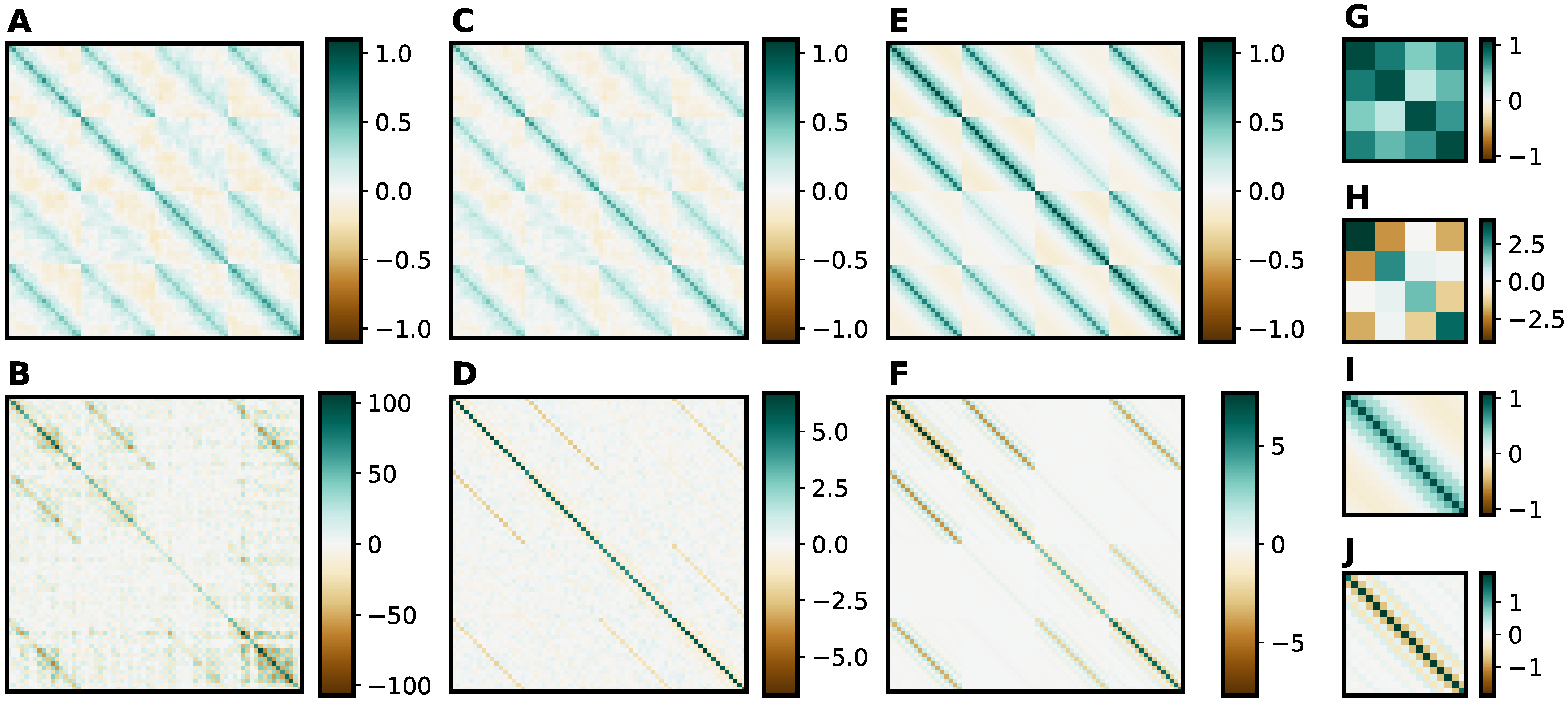
2.3. Covariance Matrix Regularization

Although the spatiotemporal beamformer, in theory, achieves optimal separation between target and non-target classes, in analogy to linear discriminant analysis [27], it does not always perform well on unseen data. The main challenge is to find a good estimator for the inverse covariance matrix C 1 since the real underlying covariance matrix generating the data is, in principle, unknown.

2.3.1. Empirical Covariance Estimation

Earlier spatiotemporal beamformer studies [21,22,28,29] use the empirical covariance and inverse covariance, calculated as follows:
C ^ emp = 1 n 1 i = 1 n x i x i
C 1 ^ emp = C ^ emp +
The Moore–Penrose pseudoinverse + ensures that a solution exists when C ^ emp is singular. Figure 1A,B show examples of the empirical estimators of the covariance and the inverse covariance matrices, respectively. The empirical estimator suffers from performance and stability issues if the number of epochs n used for estimation is not much larger than the number of features c s [30,31].

2.3.2. Shrunk Covariance Estimation

The shrinkage covariance estimator creates a better-conditioned inversion matrix problem and generally performs better when applied to unseen data. The estimators for the covariance and inverse covariance are given by:
C ^ α = ( 1 α ) C ^ emp + α Tr ( C ^ emp ) c s I
C 1 ^ α = C ^ α +
with 0 < α < 1 . Analogous to L2 regularization of the beamforming problem, shrinkage reduces the ratio between the smallest and largest eigenvalues of the covariance matrix by strengthening the diagonal. Figure 1C,D show examples of the shrunk estimator of the covariance and the inverse covariance matrices, respectively.
Earlier work [23] applied shrinkage regularization to ERP decoding with the spatiotemporal beamformer and showed competitive performance compared to other state-of-the-art decoding techniques such as stepwise LDA or SVM. The abovementioned researchers chose the shrinkage coefficient α as a fixed hyperparameter. However, its optimal value depends on the number of training epochs, the covariance matrix’s dimensionality, and the independence and variance of the data, which can vary across evaluation settings and per session. The optimal value for α can be found with a line search using cross-validation method, but this can be a costly procedure. Methods exist to estimate an optimal shrinkage value directly from the data. Most notable among these are the Ledoit–Wolf procedure [32], the Rao–Blackwell Ledoit–Wolf method [33], and the oracle approximating shrinkage method [33]. A more recent estimation method [34] emulates a leave-one-out cross-validation (LOOCV) scheme expressed by the data-driven closed-form estimate:
α = 1 n n 1 Tr ( C ^ emp 2 ) 2 c s Tr ( C ^ emp ) 2 + 1 c s Tr ( C ^ emp 2 ) 1 n ( n 1 ) i = 1 n | | x i | | 2 4 n 2 2 n ( n 1 ) 2 Tr ( C ^ emp 2 ) 2 c s Tr ( C ^ emp ) 2 + 1 c s Tr ( C ^ emp 2 ) + 1 n ( n 1 ) 2 i = 1 n | | x i | | 2 4
Herein, we opt for the LOOCV shrinkage estimator because it avoids some of the assumptions made by [32,33] and because it generalizes to structured covariance estimations, as described in Section 2.3.3.

2.3.3. Spatiotemporal Beamforming with Kronecker–Toeplitz-Structured Covariance

Exploiting prior knowledge about the spatiotemporal structure of the EEG signal leads to a more regularized estimator of the covariance. When viewing the example of empirical spatiotemporal EEG covariance in Figure 1a, it becomes clear that this matrix consists of a block pattern of repeated, similar matrices. Due to the multi-channel nature of the signal, we assume that the covariance of spatiotemporal EEG epochs is a Kronecker product of two smaller matrices [35,36,37], as expressed by:
C ^ struct = S ^ T ^
with ⊗ denoting the Kronecker product operator. S ^ R c × c and T ^ R s × s correspond to estimators of the spatial and temporal covariance of the data, respectively. Furthermore, because the temporal covariance of the EEG-signal is stationary (i.e., it is only dependent on interval length between covarying time samples) [38], it is assumed to have a Toeplitz-matrix structure:
t ^ i , j = t ^ i + 1 , j + 1
Property 1 then leads to Equation (13) to estimate the inverse covariance.
Property 1. ( U V ) + = U + V + for any non-singular matrices U and V [39].
C 1 ^ struct = S ^ + T ^ +
Finally, based on Property 2, Equation (4) can be reformulated more efficiently as Equation (14).
Property 2. ( U V ) · v e c ( W ) = v e c ( V W U ) for any matrices U R p × p , V R q × q , and W R p × q [40].
w ^ struct = S ^ + A T T ^ + a · vec ( S ^ + A T T ^ + )
Using Equation (14) removes the need to calculate the full, high-dimensional Kronecker product S ^ + T ^ + . Figure 1E,F show examples of the structured covariance and inverse covariance estimators, respectively, consisting of a spatial Kronecker factor (Figure 1G,H) and a temporal component (Figure 1I,J).
The Kronecker approach has shown significant performance yields in different linear spatiotemporal EEG and MEG applications [24,37,41,42,43]. Van Vliet and Salmelin [25] applied a Kronecker-structured covariance estimator to ERP classification with linear models in a post hoc fashion. Our work goes further by embedding the Kronecker structure in the spatiotemporal beamformer training process, using a data-adaptive shrinkage method, and regularizing the covariance further by imposing a Toeplitz structure on the temporal covariance.

2.3.4. Kronecker–Toeplitz-Structured Covariance Estimation

The question remains how to estimate S ^ and T ^ . Although the flip-flop and non-iterative flip-flop algorithms [44,45,46] can estimate Kronecker or Kronecker–Toeplitz-structured covariances, new results show that a fixed point iteration is more efficient [47,48]. After each iteration, the spatial and temporal covariance matrices are scaled to unit variance to ensure that the fixed-point iteration converges. Finally, shrinkage can also be introduced in the fixed-point iteration to improve stability and achieve more robust regularization [42,48,49,50].
The spatial and temporal covariance matrices are shrunk at every fixed-point iteration with shrinkage factors β k and γ k before matrix inversion in the next iteration. Combined, this leads to the iterative estimation algorithm described by the following equations:
S ˜ k + 1 = 1 n i = 1 n X i T ^ k + X i
T ˜ k + 1 = 1 n i = 1 n X i S ^ k + X i
S ˜ k + 1 ( β ) = ( 1 β k + 1 ) S ˜ k + 1 + β k + 1 Tr ( S ˜ k + 1 ) c I
T ˜ k + 1 ( γ ) = ( 1 γ k + 1 ) T ˜ k + 1 + γ k + 1 Tr ( T ˜ k + 1 ) s I
S ^ k + 1 = c Tr S ˜ k + 1 ( β ) S ˜ k + 1 ( β )
T ^ k + 1 = s Tr T ˜ k + 1 ( γ ) T ˜ k + 1 ( γ )
S ^ 0 and T ^ 0 can be initialized to any positive definite matrix. We choose to use the identity matrices I c × c and I s × s . After each iteration, all diagonals of R ^ k + 1 are set to their mean values to ensure that R ^ k + 1 and T ^ k + 1 are Toeplitz-structured.
Xie et al. [51] show that the LOOCV estimates for the optimal values of β k + 1 and γ k + 1 also yield a closed-form solution for the Kronecker fixed-point-iteration algorithm:
β k + 1 = 1 n n 1 Tr ( S ˜ k + 1 2 ) 2 c Tr ( S ˜ k + 1 ) 2 + 1 c Tr ( S ˜ k + 1 2 ) 1 n ( n 1 ) i = 1 n Tr ( X i T ^ k + X i ) 2 n 2 2 n ( n 1 ) 2 Tr ( S ˜ k + 1 2 ) 2 c Tr ( S ˜ k + 1 ) 2 + 1 c Tr ( S ˜ k + 1 2 ) + 1 n ( n 1 ) 2 i = 1 n Tr ( X i T ^ k + X i ) 2
γ k + 1 = 1 n n 1 Tr ( T ˜ k + 1 2 ) 2 s Tr ( T ˜ k + 1 ) 2 + 1 s Tr ( T ˜ k + 1 2 ) 1 n ( n 1 ) i = 1 n Tr ( X i S ^ k + X i ) 2 n 2 2 n ( n 1 ) 2 Tr ( T ˜ k + 1 2 ) 2 s Tr ( T ˜ k + 1 ) 2 + 1 s Tr ( T ˜ k + 1 2 ) + 1 n ( n 1 ) 2 i = 1 n Tr ( X i S ^ k + X i ) 2
The shrinkage parameters 0 < β k + 1 < 1 and 0 < γ k + 1 < 1 should be re-determined after each iteration. The oracle approximation shrinkage method can also be used to determine β k + 1 and γ k + 1 [51,52] but performs worse for spatiotemporal EEG data since not all assumptions are met.

2.4. Dataset

We use the dataset from [21], containing P300 oddball EEG recordings of 21 healthy subjects since it is a high-quality dataset with a high number (32) of electrodes and concurrently recorded EOG responses for ocular artifact rejection. Nine targets were arranged on a monitor in front of the subject during an experimental session. The subject was asked to pay attention to a cued target for a block of stimulations. Within each block, the stimulations were organized in in 15 separate subsequent trials. A trial was defined as 9 stimulations in which each target is flashed precisely once per trial. Each target was cued four times, resulting in a dataset consisting of 36 blocks (4860 stimulations) per subject. Each stimulation corresponded to a single epoch in the preprocessed dataset. See [21] for a complete description of the dataset and the recording procedure.

2.5. Software and Preprocessing

Data processing and classifier analysis were performed in Python using Scikit-Learn (version 1.0.1) [53] and SciPy (version 1.7.1) [54]. The preprocessing pipeline was implemented using the MNE-Python toolbox (version 0.24.0) [55]. The dataset was converted to BIDS-EEG format [56] and managed and loaded with MNE-BIDS (version 0.9) [57]. The Riemannian classifier from Section 2.6.3 was implemented using pyRiemann (version 0.2.7). Statistical tests were performed in R (version 4.1.2).
The EEG recorded at 2048 Hz was re-referenced off-line to the average of the mastoids. The reference electrodes were dropped from the analysis. Data were subsequently filtered between 0.5Hz and 16Hz using forward-backward filtering with a fourth-order Butterworth IIR filter. The EEG signal was corrected for ocular artifacts using independent component analysis (ICA) by rejecting components that correlated with the bipolar EOG channels vEOG and hEOG, according to adaptive Z-score thresholding. Finally, epochs were cut from 0.1 s to 0.6 s after stimulus onset. No baseline correction was performed since this affects the temporal covariance of the data, violating the Toeplitz structure assumption [38].

2.6. Classification

2.6.1. Cross-Validation Scheme per Subject

We use a variation of grouped k-fold cross-validation per subject to evaluate the classifiers. We applied four-fold cross-validation by splitting the blocks of each subject into four continuous folds. Unlike regular cross-validation, we only used a single fold to train the classifiers while using the other three folds for validation. This scheme resulted in a training set of 9 blocks of 135 epochs each. We chose this approach since we are primarily interested in the performance of the classifiers in the case of low data availability. The classification task was to determine the cued target for each block. The fraction of correctly predicted cues provided the accuracy of a classifier. Data from all trials were used in the training stage, whereas classifier validation was performed multiple times per fold, each time using an increasing amount of trials (i.e., using the first trial, using the first two trials, etc., until all 15 trials have been used). For each of the 9 stimulated targets, the averages over the corresponding epochs across the utilized trials were used to predict the cued target in that block. The target with the maximum classifier score was then chosen as the predicted cued target. Before training the classifiers, a Z-score normalization transformation was developed on the training data to scale all EEG channels to unit variance. This transformation was then applied to the validation data.

2.6.2. Spatiotemporal Beamformer Classifier

Before calculating the spatiotemporal beamformer (STBF), the signal was downsampled to 32 Hz or twice the low-pass frequency 16 Hz, resulting in 17 time samples between 0.1 s and 0.6 s. According to the Nyquist theorem, more samples would not contain more information; hence, the minimum temporal resolution was chosen to reduce the dimensionality of the covariance. The activation pattern is the difference between the averages of epochs in response to cued targets and the averages of those in response to non-cued targets. We constructed three variations of the spatiotemporal beamformer: STBF with empirical covariance estimation (stbf-emp) as in Section 2.3.1, STBF with LOOCV-shrunk covariance estimation (stbf-shrunk) as in Section 2.3.2, and STBF with Kronecker–Toeplitz-structured covariance estimation (stbf-struct) with LOOCV shrinkage for the Kronecker factors as in Section 2.3.4.

2.6.3. Riemannian Geometry Classifier

We opted for a Riemannian geometry-based classifier to compare our results. The Riemannian model (xdawn+rg) uses the xDAWN spatial filter combined with Riemannian geometry in tangent space as implemented by Barachant et al. [58]. This classifier uses four xDAWN spatial filters and each epoch’s empirical spatial covariance matrix. The target with the maximum score is the prediction of the cued target. xdawn+rg was trained and validated without downsampling using epochs at the original sample rate of 2048 Hz.

3. Results

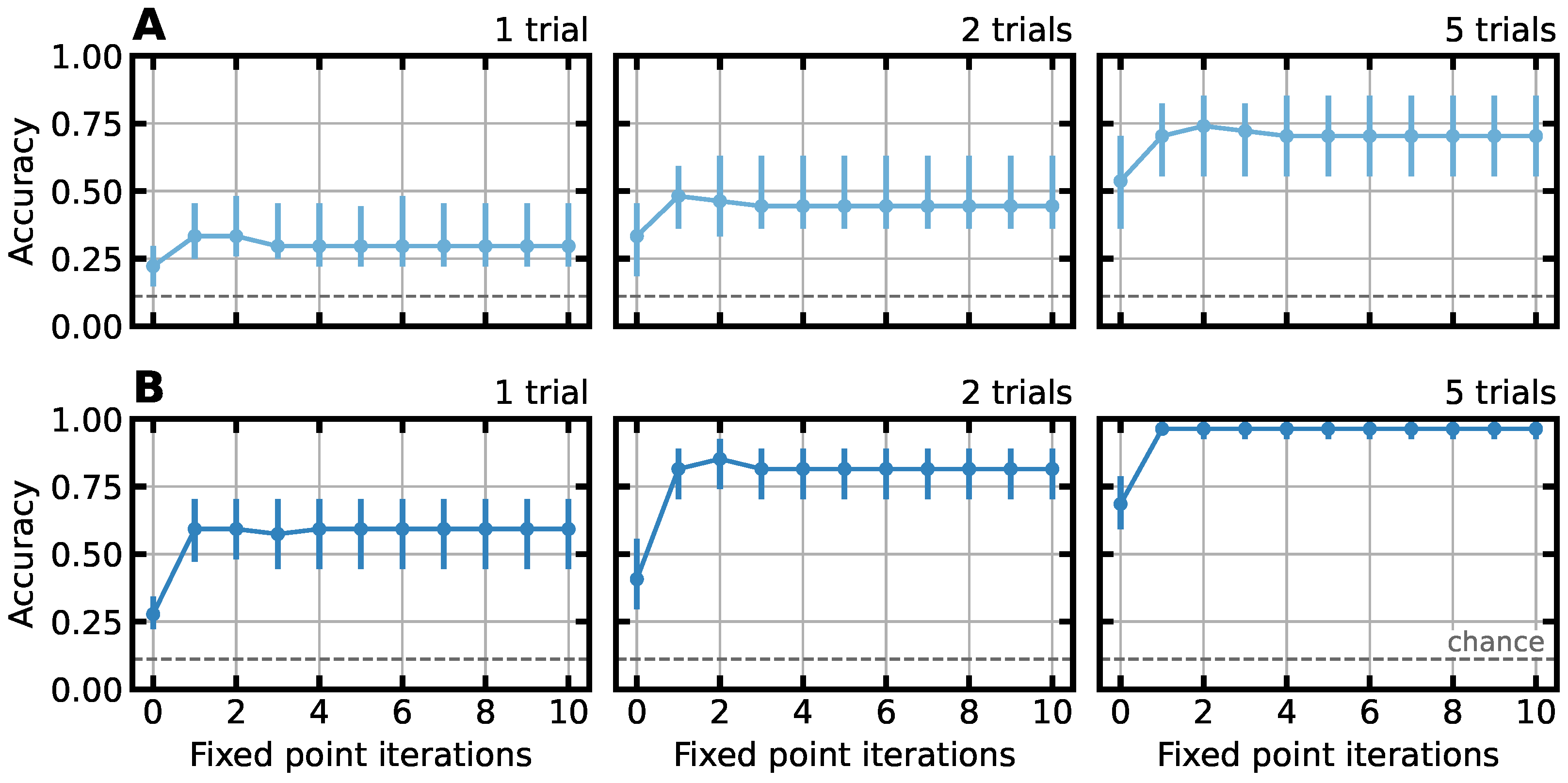
3.1. Minimum Required Fixed-Point Iterations

The fixed point iteration algorithm described in Equations (15a)–(16b) is used to estimate the Kronecker–Toeplitz-structured covariance for the stbf-struct classifier. Fixed-point iteration is an iterative procedure starting from (in our case) non-informed initial guesses for the spatial and temporal covariance matrices. As a stopping criterion, one could impose a threshold on the difference in outcome of successive steps, e.g., based on the covariance norm or the classifier accuracy. However, few iterations or even just one [59] suffice to achieve satisfactory performance in practice.
Figure 2 confirms these results for the stbf-struct classifier. Using more than one fixed-point iteration does not significantly improve the accuracy across the amounts of training data and the number of trials used for evaluation. Hence, only one iteration is used for the stbf-struct classifier, leading to a drastic speed-up of the training process.

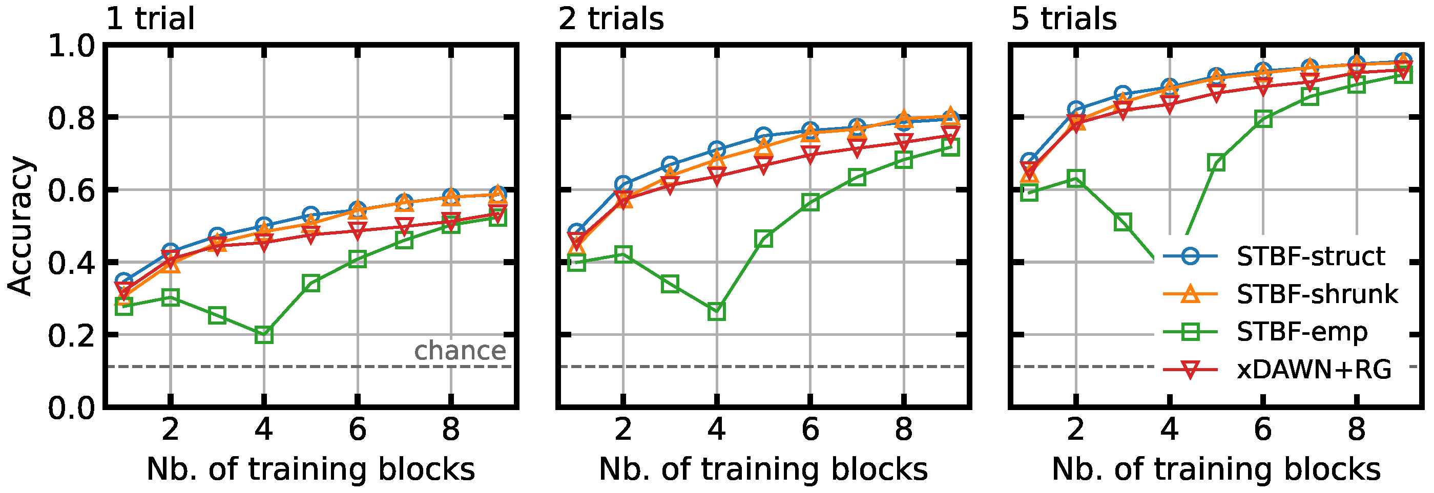
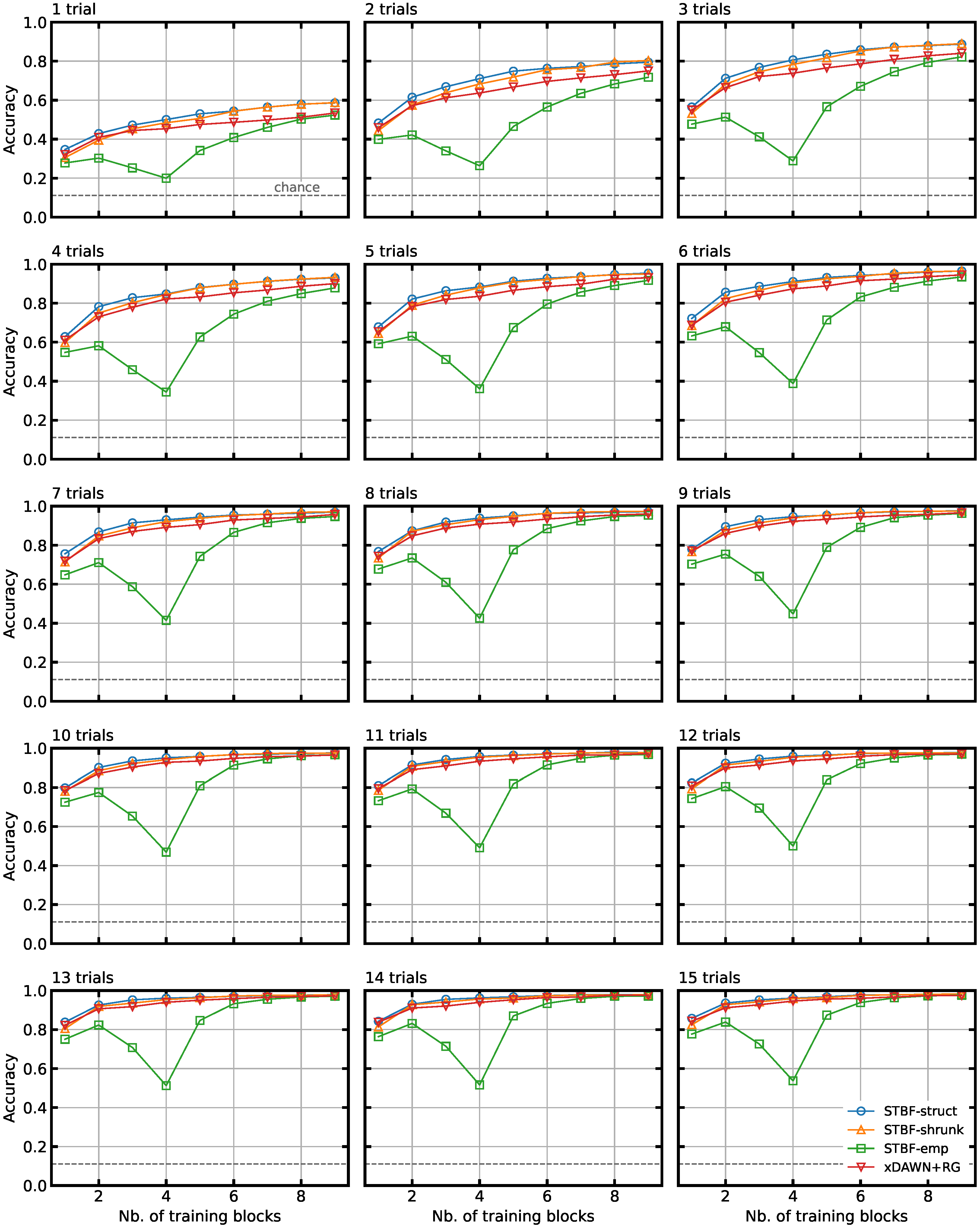
3.2. Classifier Accuracy for Limited Training Data

It is of interest to keep the calibration time before BCI operation as short as possible. We mimic this problem by training the classifier with as few training epochs as possible. We evaluate the performance of all classifiers for different levels of available training data and apply the cross-validation procedure nine times (the number of blocks in the training fold) for all subjects, keeping the corresponding number of blocks in the training folds and dropping the rest. Figure 3 and Figure A1 show each classifier’s accuracy relative to the data availability. We statistically compare the two newly proposed classifiers, stbf-struct and stbf-shrunk, for different levels of training data availability using a one-sided paired Wilcoxon rank-sum test with Holm correction for the multiple pairwise comparisons between classifiers. We performed this analysis three times: by only using the first trial of a block, by averaging epochs across the first two trials of a block, and across the first five trials of a block. Results validated on one trial are reported in Table 1, two-trial results in Table 2, and five-trial results in Table 3.
The tables show that stbf-struct has a significant advantage over stbf-shrunk when the number of training blocks is low. This effect is present for 1-, 2-, and 5-trial evaluations. This advantage decreases (the p-value increases) when adding more training blocks. Both stbf-struct and stbf-shrunk perform significantly better than stbf-emp for all evaluated settings. Compared to xdawn+rg, stbf-struct also has significantly higher accuracy in almost all evaluated settings, except when using only one training block. stbf-shrunk does not outperform xdawn+rg when training data are scarce but gains a significant advantage when using more training data.

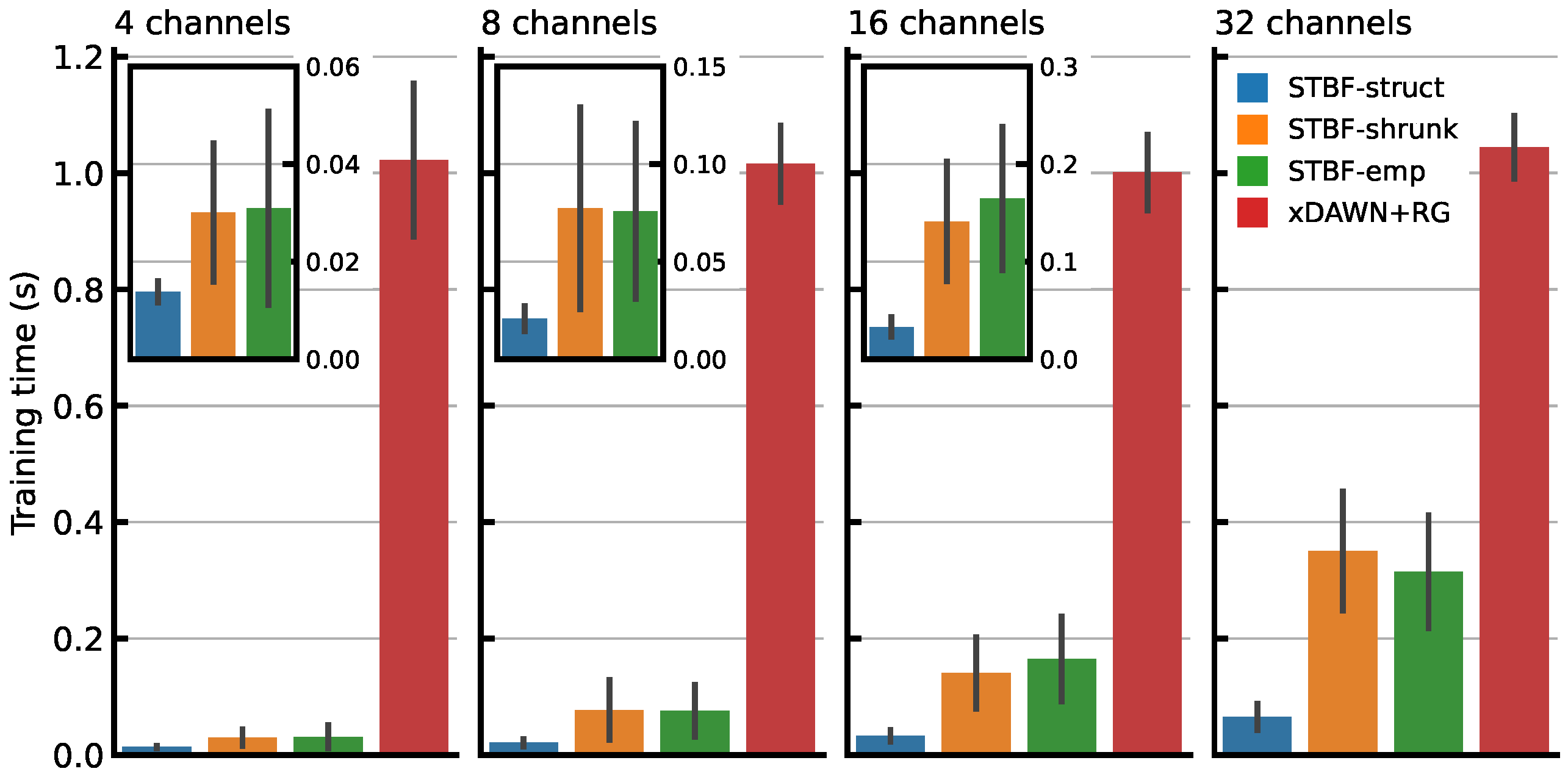
3.3. Classifier Training Time

In order to evaluate the training time of the investigated classifiers, the cross-validation scheme was run four times for each subject, each time with an increasing number of EEG channels retained in the analysis, to explore the scalability of each classifier for analyses with higher spatial resolutions. The temporal resolutions were not varied, but we expect that increasing the temporal resolution has a similar effect on training time, since the training times for the STBF-based classifiers are primarily dependent on the number of parameters in their respective covariance matrix estimators, as evidenced by the complexity calculations in Section 4.2. Figure 4 shows the measured training times. These results were obtained using a laptop with an Intel® Core™ i7-8750H CPU (Intel Corporation, Santa Clara, CA, USA) and 16 GB of RAM.
Figure 4 shows that the training time of stbf-struct increased less steeply than that of stbf-shrunk and stbf-emp. The training time of all three STBF-based classifiers was much lower than that of xdawn+rg, which appears nearly constant when using 4, 8, 16, or 32 channels.

4. Discussion

4.1. Classification Accuracy

As evidenced by Figure 3 and Table 1, Table 2 and Table 3, the regularized classifiers stbf-shrunk and stbf-struct significantly improve the classification accuracy compared to the original stbf-emp for all the numbers of training blocks indicated. We believe there are three reasons for this. First and foremost, the empirical covariance matrix in stbf-emp becomes ill-conditioned when the number of available training epochs is smaller than the number of features ( n < c s ), rendering its inversion with the Moore–Penrose pseudoinverse unstable. This is the case for stbf-emp when n = c s = 32 × 17 = 544 , after which the accuracy of stbf-emp starts to increase. This effect is visible in Figure 3, where the accuracy starts increasing when using more than four training blocks, amounting to 540 epochs. The noticeable dip in accuracy when using around 540 epochs can be explained by numerical effects in the pseudoinverse for very small eigenvalues [60,61,62,63]. Regularization of the covariance matrix with shrinkage ensures that the covariance matrix is non-singular and better conditioned so that it can stably be inverted. Second, covariance regularization introduces a trade-off between the variance and bias of the model [32]. Better performance on unseen data can be achieved when some model variance is traded for extra bias. Regularization reduces the extreme values present, as shown in Figure 1, resulting in a classifier with better generalization. Third, the true spatiotemporal covariance matrix may vary throughout BCI sessions, e.g., due to movement of the EEG-cap, changing impedances of electrodes, subject fatigue, the introduction of new spatiotemporal noise sources, and other possible confounds. A regularized covariance matrix should better account for changes in true covariance. Note that the LOOCV method in principle assumes that the covariances of the training data and unseen data are the same. Because the covariance might have changed for unseen data, the shrinkage estimate obtained with LOOCV is probably still an underestimation of the optimal—but unknown—shrinkage coefficient that would yield the best classification accuracy for the unseen data.
Another observation is the significantly better accuracy score of stbf-struct over stbf-shrunk when the amount of available training data is small. This property is an attractive advantage in a BCI setting since it is desirable to keep the calibration (training) phase as short as possible without losing accuracy. The accuracy advantage of the structured estimator is a consequence of the Kronecker–Toeplitz covariance structure, which is informative for the underlying process generating the epochs, if it is assumed that the EEG signal is a linear combination of stationary activity generated by random dipoles in the brain with added noise [24,35,41]. Hence, stbf-struct can utilize this prior information to better estimate the inverse covariance. The increase in accuracy for small training set sizes can also be explained by the smaller number of parameters necessary to estimate the inverse covariance (see Section 4.2), increasing the stability of matrix inversions.
When compared to the state-of-the-art xdawn+rg classifier, we conclude that stbf-struct reaches similar accuracy when using only one block of training data. The authors suspect this is due to both classifiers having insufficient training information to reach satisfactory classification accuracy. When more data are available, stbf-struct reaches significantly better accuracies. Combined with the benefits laid out in Section 4.2 and Section 4.3, this makes it an attractive option for ERP classification. stbf-shrunk does not show decisive accuracy improvements over xdawn+rg using a few training blocks, but this improves as the training data increases.

4.2. Time and Memory Complexity

As mentioned above, inverting the full c s × c s dimensional covariance matrix to construct stbf-emp and stbf-shrunk can be costly and unstable, in particular in high-resolution settings with many EEG channels or time samples. Constructing the full covariance and inverse covariance matrices also requires a considerable amount of memory. The structured covariance estimator of stbf-struct has two advantages here.
First, because of Properties 1 and 2 there is no need to calculate the full c s × c s symmetric covariance and inverse covariance matrices for stbf-struct or keep them in memory; they can instead be replaced by two smaller symmetric matrices of dimensions c × c and s × s , respectively. Furthermore, since the temporal component of the Kronecker product is Toeplitz-structured, it only requires s parameters to estimate. Although the inverse covariance of stbf-emp and stbf-shrunk is defined by c s ( c s + 1 ) 2 = 32 × 17 ( 32 × 17 + 1 ) 2 = 122.128 parameters accounting for the symmetric nature of covariance, the structured estimator only requires c ( c + 1 ) 2 + s = 32 ( 32 + 1 ) 2 + 17 = 545 unique parameters. This reduction in parameters to estimate reduces memory usage and contributes to the regularization effect for low-data-availability settings. The inverse covariances of stbf-emp and stbf-struct, represented as 32 × 17 × 32 × 17 symmetric matrices of single-precision real floating point numbers for weight calculation, use 9.03 MiB of memory. The 32 × 32 and 17 × 17 matrices of stbf-struct only require 5.12 KiB.
Second, structured estimation has better time complexity. Covariance estimation and inversion occupy the largest part of the STBF training time. For stbf-emp and stbf-shrunk, the time complexity of this process is O ( n c 2 s 2 + c 3 s 3 ) . Thanks to Property 1, the complexity can be reduced to O ( n c 2 s 2 + c 3 + s 3 ) for the structured estimator of stbf-struct. The results presented in Figure 4 confirm these calculations. It can be observed that the training time of stbf-struct stays low compared to stbf-emp and stbf-shrunk when dimensionality increases.
The results shown in Figure 4 also confirm that the STBF-based estimators are very fast to train compared to the state-of-the-art estimator xdawn+rg, which confirms the results in [21]. Since the training times of all STBF-based classifiers are already of the order of tenths of seconds, the question arises as to whether the improvements achieved using the structured estimator would be relevant in practice. However, the authors believe that these results could significantly impact some use-cases of the spatiotemporal beamformer, such as high-spatial- or temporal-resolution ERP analyses. One example is single-trial ERP analysis with a high temporal resolution to extract ERP time features. Such higher-resolution analyses can later be incorporated into an ERP classification framework. In addition, the speed provided by structured estimation yields a faster off-line evaluation of the STBF ERP classifier, in which multiple cross-validation folds, subjects, and hyperparameter settings often need to be explored, which can quickly increase runtime. Improvements in computation speed and memory usage can remove the need for dedicated computation hardware and enable group analyses to be run on a personal computer.

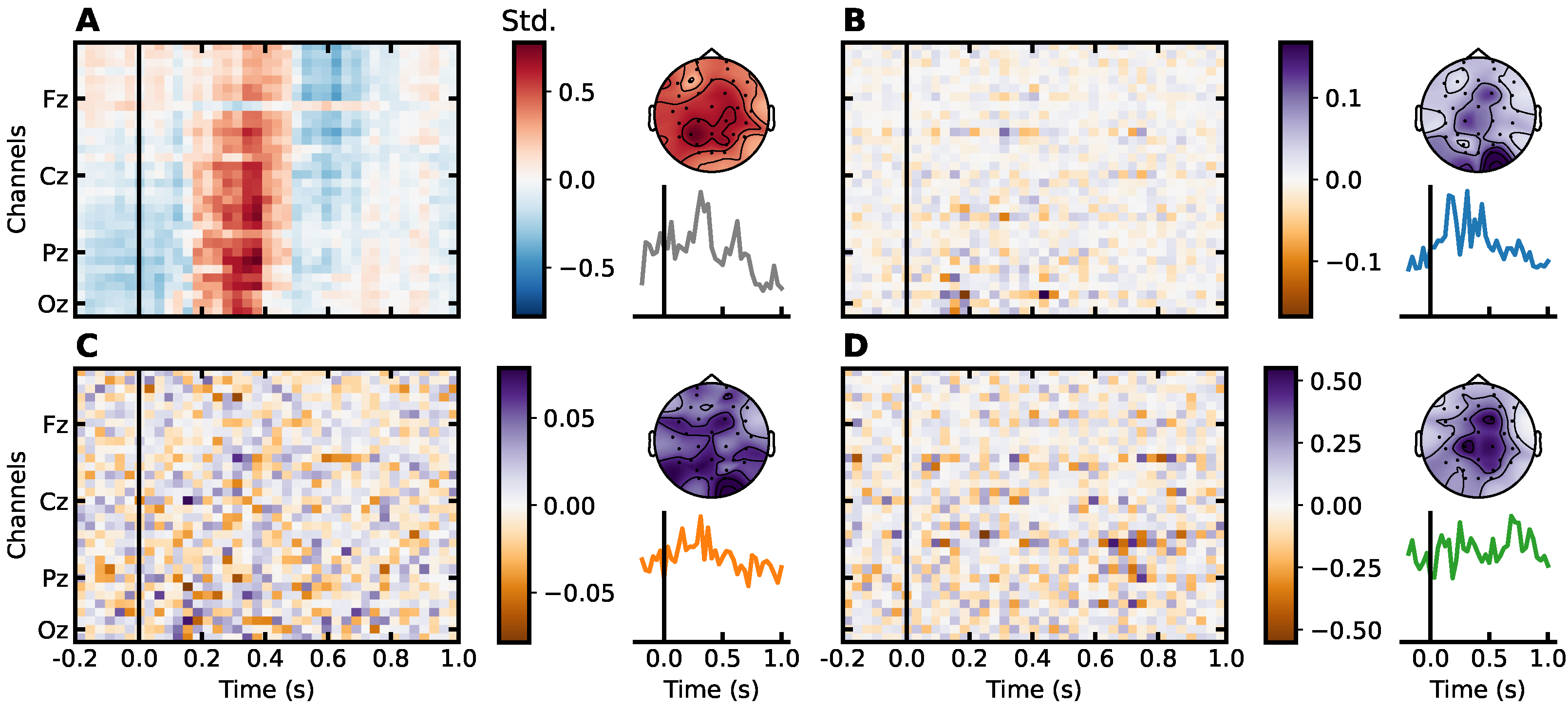
4.3. Interpreting the Weights

The weight matrix of the STBF determines how each spatiotemporal feature of a given epoch should contribute to enhancing the SNR of the discriminating signal in the classification task. Alternatively, the activation pattern can be regarded as a forward EEG model of the activity, generating the discriminating signal and the weights as a backward model [60,64]. Regularization enables a researcher to interpret better the distribution of the weight over space and time after reshaping the weight vector w to its spatiotemporal matrix equivalent, W, such that vec ( W ) = w . Figure 5 compares the weights calculated in stbf-emp and stbf-shrunk with the weights from stbf-struct.
Since the linear filter’s noise suppression and signal amplification functions are deeply entangled, it is not necessarily true that features with a high filter weight directly correlate to features containing discriminatory information [64]. However, it is still possible to interpret the weights in terms of which features contribute most to the classification process, be it through noise suppression, signal amplification, or—most likely—a combination of both. The weights obtained by stbf-emp seem to be randomly distributed over space and time; the regularized estimator used by stbf-shrunk and stbf-struct reveal a more interpretable weight distribution. The stbf-shrunk weights show a sparse spatial distribution, whereas the stbf-struct weights show a sparse distribution in both space and in time.
As expected, Figure 5b and d exhibit weight around the central and parietal regions, where the P300 ERP component is present. Especially the spatial weights of stbf-shrunk in Figure 5d correspond to the spatial activation pattern in Figure 5a. This is not surprising, since shrinkage transforms the covariance matrix closer to the identity matrix and assuming identity covariance in Figure 4 yields weights identical to the activation pattern (up to a scaling factor). Additionally, Figure 5b shows that weights in the baseline interval and after 0.6 s, which should contain no response information, are close to zero for the structured estimator. Meanwhile, these weights are high in the occipital region between 0.1 s and 0.2 s, containing early visual components with relatively low SNR. This high weight for the early visual components confirms the results from Treder and Blankertz [65] that state that, in addition to the P300, the early N1 and P2 ERP components are also modulated by oddball attention and contain discriminatory information between attended and non-attended stimuli.
Using an interpretable classification model has many advantages. For instance, one can use the weight matrix to determine relevant time samples and EEG channels for per-subject feature selection to refine the model further. The number of channels is also an important cost factor in practical BCI applications. Determining which channels do not contribute to the classification accuracy helps to reduce the number of required electrodes. Spatially clustered weights indicate that some electrodes are not used by the classifier and can be discarded accordingly with no substantial accuracy reduction. As another example, information about the timing and spatial distribution of the discriminatory information in the response can be extracted from the weights and linked to neurophysiological hypotheses.

5. Conclusions

Although it is possible to regularize the spatiotemporal LCMV beamformer classifier for ERP detection through other methods, such as by employing feature selection, by adding regularizing penalties to the cost function beamforming problem, or by crafting a cleaner activation pattern, our work focused on estimation methods for spatiotemporal covariance. We introduced a covariance estimator using adaptive shrinkage and an estimator exploiting prior knowledge about the spatiotemporal nature of the EEG signal. We compared these estimators with the original spatiotemporal beamformer and a state-of-the-art method in an off-line P300 detection task. Our results show that the structured estimator performs better when training data are sparsely available and that results can be computed faster and with substantially less memory usage. Since these algorithms are not paradigm-specific, the conclusions can be generalized to other ERP-based BCI settings.
Future work should focus on introducing more robust regularization strategies using prior knowledge, such as shrinking the spatial covariance to a population mean or a previously known matrix based on sensor geometry or characterizing the temporal covariance as a wavelet or autoregressive model. More accurate results could be obtained by expressing the covariance as the sum of multiple Kronecker products to account for spatial variation in temporal covariance. It could also be interesting to explore the impact of covariance regularization on transfer learning of the STBF between subjects to alleviate calibration entirely. Finally, it could be insightful to evaluate the proposed algorithms in a real-world on-line BCI setting.

Author Contributions

Conceptualization, A.V.D.K.; methodology, A.V.D.K., A.L., B.W. and M.M.V.H.; software, A.V.D.K., validation, A.V.D.K.; formal analysis, A.V.D.K. and B.W.; investigation, A.V.D.K. and B.W.; resources, M.M.V.H. and B.W.; data curation, A.V.D.K.; writing—original draft preparation, A.V.D.K.; writing—review and editing, A.V.D.K., A.L., B.W. and M.M.V.H.; visualization, A.V.D.K.; supervision, M.M.V.H.; project administration, A.V.D.K. and M.M.V.H.; funding acquisition, M.M.V.H. All authors have read and agreed to the published version of the manuscript.

Funding

A.V.D.K. is supported by the special research fund of the KU Leuven (GPUDL/20/031). A.L. is supported by the Belgian Fund for Scientific Research—Flanders (1SC3419N). M.M.V.H. is supported by research grants received from the European Union’s Horizon 2020 research and innovation programme under grant agreement No. 857375, the special research fund of the KU Leuven (C24/18/098), the Belgian Fund for Scientific Research—Flanders (G0A4118N, G0A4321N, G0C1522N), and the Hercules Foundation (AKUL 043).

Institutional Review Board Statement

The study was conducted according to the guidelines of the Declaration of Helsinki, and approved by the Ethics Committee of KU Leuven’s university hospital (UZ Leuven) (S62547 approved 11 June 2019).

Informed Consent Statement

Informed consent was obtained from all subjects involved in the study.

Data Availability Statement

No new data were created or analyzed in this study. Data sharing is not applicable to this article. Source code is available at https://github.com/kul-compneuro/stbf-erp (accessed 7 March 2022).

Acknowledgments

The authors acknowledge François Cabestaing and Hakim Si-Mohammed for their valuable input in the development of this article.

Conflicts of Interest

The authors declare no conflict of interest. The funders had no role in the design of the study; in the collection, analyses, or the interpretation of data; in the writing of the manuscript, or in the decision to publish the results.

Appendix A

Figure A1. Accuracy of the different classifiers for all 21 subjects relative to the number of blocks available for training. One block consists of 135 epochs and corresponds to 27 s of stimulation. Accuracies are shown for the evaluation settings, averaging over different numbers of trials, ranging from 1 to 15.
Applsci 12 02918 g0a1

References

  1. Wolpaw, J.R.; Birbaumer, N.; McFarland, D.J.; Pfurtscheller, G.; Vaughan, T.M. Brain–computer interfaces for communication and control. Clin. Neurophysiol. 2002, 113, 767–791. [Google Scholar] [CrossRef]
  2. Naci, L.; Monti, M.M.; Cruse, D.; Kübler, A.; Sorger, B.; Goebel, R.; Kotchoubey, B.; Owen, A.M. Brain–computer interfaces for communication with nonresponsive patients. Ann. Neurol. 2012, 72, 312–323. [Google Scholar] [CrossRef] [PubMed]
  3. Chaudhary, U.; Birbaumer, N.; Ramos-Murguialday, A. Brain-computer interfaces for communication and rehabilitation. Nat. Rev. Neurol. 2016, 12, 513–525. [Google Scholar] [CrossRef] [PubMed] [Green Version]
  4. Abiri, R.; Borhani, S.; Sellers, E.W.; Jiang, Y.; Zhao, X. A comprehensive review of EEG-based brain–computer interface paradigms. J. Neural Eng. 2019, 16, 11001. [Google Scholar] [CrossRef] [PubMed]
  5. Mellinger, J.; Schalk, G.; Braun, C.; Preissl, H.; Rosenstiel, W.; Birbaumer, N.; Kübler, A. An MEG-based brain–computer interface (BCI). NeuroImage 2007, 36, 581–593. [Google Scholar] [CrossRef] [PubMed] [Green Version]
  6. Hong, K.S.; Naseer, N.; Kim, Y.H. Classification of prefrontal and motor cortex signals for three-class fNIRS–BCI. Neurosci. Lett. 2015, 587, 87–92. [Google Scholar] [CrossRef] [PubMed]
  7. Paek, A.Y.; Kilicarslan, A.; Korenko, B.; Gerginov, V.; Knappe, S.; Contreras-Vidal, J.L. Towards a Portable Magnetoencephalography Based Brain Computer Interface with Optically-Pumped Magnetometers. In Proceedings of the 2020 42nd Annual International Conference of the IEEE Engineering in Medicine Biology Society (EMBC), Montreal, QC, Canada, 20–24 July 2020; pp. 3420–3423. [Google Scholar] [CrossRef]
  8. Schalk, G.; Leuthardt, E.C. Brain-computer interfaces using electrocorticographic signals. IEEE Rev. Biomed. Eng. 2011, 4, 140–154. [Google Scholar] [CrossRef] [PubMed]
  9. Maynard, E.M.; Nordhausen, C.T.; Normann, R.A. The Utah Intracortical Electrode Array: A recording structure for potential brain-computer interfaces. Electroencephalogr. Clin. Neurophysiol. 1997, 102, 228–239. [Google Scholar] [CrossRef]
  10. Willett, F.R.; Avansino, D.T.; Hochberg, L.R.; Henderson, J.M.; Shenoy, K.V. High-performance brain-to-text communication via handwriting. Nature 2021, 593, 249–254. [Google Scholar] [CrossRef]
  11. Gao, S.; Wang, Y.; Gao, X.; Hong, B. Visual and Auditory Brain–Computer Interfaces. IEEE Trans. Biomed. Eng. 2014, 61, 1436–1447. [Google Scholar] [CrossRef]
  12. Kapgate, D.; Kalbande, D. A Review on Visual Brain Computer Interface. In Advancements of Medical Electronics; Lecture Notes in Bioengineering; Gupta, S., Bag, S., Ganguly, K., Sarkar, I., Biswas, P., Eds.; Springer India: New Delhi, India, 2015; pp. 193–206. [Google Scholar] [CrossRef]
  13. Farwell, L.A.; Donchin, E. Talking off the top of your head: Toward a mental prosthesis utilizing event-related brain potentials. Electroencephalogr. Clin. Neurophysiol. 1988, 70, 510–523. [Google Scholar] [CrossRef]
  14. Sellers, E.W.; Donchin, E. A P300-based brain–computer interface: Initial tests by ALS patients. Clin. Neurophysiol. 2006, 117, 538–548. [Google Scholar] [CrossRef] [PubMed]
  15. Barachant, A.; Congedo, M. A Plug&Play P300 BCI Using Information Geometry. arXiv 2014, arXiv:1409.0107. [Google Scholar]
  16. Philip, J.T.; George, S.T. Visual P300 Mind-Speller Brain-Computer Interfaces: A Walk through the Recent Developments with Special Focus on Classification Algorithms. Clin. EEG Neurosci. 2020, 51, 19–33. [Google Scholar] [CrossRef] [PubMed]
  17. Tayeb, S.; Mahmoudi, A.; Regragui, F.; Himmi, M.M. Efficient detection of P300 using Kernel PCA and support vector machine. In Proceedings of the 2014 Second World Conference on Complex Systems (WCCS), Agadir, Morocco, 10–12 November 2014; pp. 17–22. [Google Scholar] [CrossRef]
  18. Vařeka, L. Evaluation of convolutional neural networks using a large multi-subject P300 dataset. Biomed. Signal Process. Control. 2020, 58, 101837. [Google Scholar] [CrossRef] [Green Version]
  19. Borra, D.; Fantozzi, S.; Magosso, E. Convolutional neural network for a P300 brain-computer interface to improve social attention in autistic spectrum disorder. In Mediterranean Conference on Medical and Biological Engineering and Computing—MEDICON 2019; Henriques, J., Neves, N., de Carvalho, P., Eds.; Springer International Publishing: Cham, Switzerland, 2020; pp. 1837–1843. [Google Scholar] [CrossRef]
  20. Van Vliet, M.; Chumerin, N.; De Deyne, S.; Wiersema, J.R.; Fias, W.; Storms, G.; Van Hulle, M.M. Single-trial erp component analysis using a spatiotemporal lcmv beamformer. IEEE Trans. Biomed. Eng. 2015, 63, 55–66. [Google Scholar] [CrossRef] [PubMed]
  21. Wittevrongel, B.; Van Hulle, M.M. Faster p300 classifier training using spatiotemporal beamforming. Int. J. Neural Syst. 2016, 26, 1650014. [Google Scholar] [CrossRef]
  22. Wittevrongel, B.; Van Hulle, M.M. Spatiotemporal Beamforming: A Transparent and Unified Decoding Approach to Synchronous Visual Brain-Computer Interfacing. Front. Neurosci. 2017, 11, 630. [Google Scholar] [CrossRef] [Green Version]
  23. Libert, A.; Wittevrongel, B.; Van Hulle, M.M. Effect of stimulus direction on motion-onset visual evoked potentials decoded using spatiotemporal beamforming Abstract. In Proceedings of the 2021 10th International IEEE/EMBS Conference on Neural Engineering (NER), Virtual, 4–6 May 2021; pp. 503–506. [Google Scholar] [CrossRef]
  24. Gonzalez-Navarro, P.; Moghadamfalahi, M.; Akçakaya, M.; Erdogmus, D. Spatio-temporal EEG models for brain interfaces. Signal Process. 2017, 131, 333–343. [Google Scholar] [CrossRef] [PubMed] [Green Version]
  25. Van Vliet, M.; Salmelin, R. Post-hoc modification of linear models: Combining machine learning with domain information to make solid inferences from noisy data. NeuroImage 2020, 204, 116221. [Google Scholar] [CrossRef]
  26. Van Veen, B.D.; Van Drongelen, W.; Yuchtman, M.; Suzuki, A. Localization of brain electrical activity via linearly constrained minimum variance spatial filtering. IEEE Trans. Biomed. Eng. 1997, 44, 867–880. [Google Scholar] [CrossRef] [PubMed]
  27. Treder, M.S.; Porbadnigk, A.K.; Avarvand, F.S.; Müller, K.R.; Blankertz, B. The LDA beamformer: Optimal estimation of ERP source time series using linear discriminant analysis. NeuroImage 2016, 129, 279–291. [Google Scholar] [CrossRef] [PubMed]
  28. Wittevrongel, B.; Hulle, M.M.V. Frequency- and Phase Encoded SSVEP Using Spatiotemporal Beamforming. PLoS ONE 2016, 11, e0159988. [Google Scholar] [CrossRef] [PubMed] [Green Version]
  29. Wittevrongel, B.; Van Wolputte, E.; Van Hulle, M.M. Code-modulated visual evoked potentials using fast stimulus presentation and spatiotemporal beamformer decoding. Sci. Rep. 2017, 7, 15037. [Google Scholar] [CrossRef] [PubMed] [Green Version]
  30. Stein, C. Inadmissability of the usual estimator for the mean of a multivariate normal distribution. In Contribution to the Theory of Statistics; University of California Press: Berkeley, CA, USA, 1956; Volume 1, pp. 197–206. [Google Scholar] [CrossRef]
  31. Khatri, C.; Rao, C. Effects of estimated noise covariance matrix in optimal signal detection. IEEE Trans. Acoust. Speech, Signal Process. 1987, 35, 671–679. [Google Scholar] [CrossRef]
  32. Ledoit, O.; Wolf, M. A well-conditioned estimator for large-dimensional covariance matrices. J. Multivar. Anal. 2004, 88, 365–411. [Google Scholar] [CrossRef] [Green Version]
  33. Chen, Y.; Wiesel, A.; Eldar, Y.C.; Hero, A.O. Shrinkage algorithms for MMSE covariance estimation. IEEE Trans. Signal Process. 2010, 58, 5016–5029. [Google Scholar] [CrossRef] [Green Version]
  34. Tong, J.; Hu, R.; Xi, J.; Xiao, Z.; Guo, Q.; Yu, Y. Linear shrinkage estimation of covariance matrices using low-complexity cross-validation. Signal Process. 2018, 148, 223–233. [Google Scholar] [CrossRef] [Green Version]
  35. De Munck, J.; Vijn, P.; Lopes da Silva, F. A random dipole model for spontaneous brain activity. IEEE Trans. Biomed. Eng. 1992, 39, 791–804. [Google Scholar] [CrossRef]
  36. De Munck, J.C.; Van Dijk, B.W. The Spatial Distribution of Spontaneous EEG and MEG; Springer Series in Synergetics; Springer: Berlin/Heidelberg, Germany, 1999; pp. 202–228. [Google Scholar] [CrossRef]
  37. Huizenga, H.M.; De Munck, J.C.; Waldorp, L.J.; Grasman, R.P. Spatiotemporal EEG/MEG source analysis based on a parametric noise covariance model. IEEE Trans. Biomed. Eng. 2002, 49, 533–539. [Google Scholar] [CrossRef]
  38. Bijma, F.; de Munck, J.C.; Huizenga, H.M.; Heethaar, R.M. A mathematical approach to the temporal stationarity of background noise in MEG/EEG measurements. NeuroImage 2003, 20, 233–243. [Google Scholar] [CrossRef] [Green Version]
  39. Langville, A.N.; Stewart, W.J. The Kronecker product and stochastic automata networks. J. Comput. Appl. Math. 2004, 167, 429–447. [Google Scholar] [CrossRef]
  40. Loan, C.F.V. The ubiquitous Kronecker product. J. Comput. Appl. Math. 2000, 123, 85–100. [Google Scholar] [CrossRef] [Green Version]
  41. De Munck, J.C.; Huizenga, H.M.; Waldorp, L.J.; Heethaar, R. Estimating stationary dipoles from MEG/EEG data contaminated with spatially and temporally correlated background noise. IEEE Trans. Signal Process. 2002, 50, 1565–1572. [Google Scholar] [CrossRef]
  42. Beltrachini, L.; von Ellenrieder, N.; Muravchik, C.H. Shrinkage Approach for Spatiotemporal EEG Covariance Matrix Estimation. IEEE Trans. Signal Process. 2013, 61, 1797–1808. [Google Scholar] [CrossRef]
  43. Gonzalez-Navarro, P.; Moghadamfalahi, M.; Akcakaya, M.; Erdogmus, D. A kronecker product structured EEG covariance estimator for a language model assisted-BCI. In International Conference on Augmented Cognition; Springer: Cham, Switzerland, 2016; pp. 35–45. [Google Scholar] [CrossRef]
  44. Lu, N.; Zimmerman, D.L. The likelihood ratio test for a separable covariance matrix. Stat. Probab. Lett. 2005, 73, 449–457. [Google Scholar] [CrossRef]
  45. Werner, K.; Jansson, M.; Stoica, P. On estimation of covariance matrices with Kronecker product structure. IEEE Trans. Signal Process. 2008, 56, 478–491. [Google Scholar] [CrossRef]
  46. Wirfält, P.; Jansson, M. On Toeplitz and Kronecker structured covariance matrix estimation. In Proceedings of the 2010 IEEE Sensor Array and Multichannel Signal Processing Workshop, Jerusalem, Israel, 4–7 October 2010; pp. 185–188. [Google Scholar] [CrossRef] [Green Version]
  47. Wiesel, A. Geodesic Convexity and Covariance Estimation. IEEE Trans. Signal Process. 2012, 60, 6182–6189. [Google Scholar] [CrossRef]
  48. Wiesel, A. On the convexity in Kronecker structured covariance estimation. In Proceedings of the 2012 IEEE Statistical Signal Processing Workshop (SSP), Ann Arbor, MI, USA, 5–8 August 2012; pp. 880–883. [Google Scholar] [CrossRef]
  49. Greenewald, K.; Hero, A.O. Regularized block Toeplitz covariance matrix estimation via Kronecker product expansions. In Proceedings of the 2014 IEEE Workshop on Statistical Signal Processing (SSP), Gold Coast, Australia, 29 June–2 July 2014; pp. 9–12. [Google Scholar] [CrossRef] [Green Version]
  50. Breloy, A.; Sun, Y.; Babu, P.; Ginolhac, G.; Palomar, D. Robust rank constrained kronecker covariance matrix estimation. In Proceedings of the 2016 50th Asilomar Conference on Signals, Systems and Computers, Pacific Grove, CA, USA, 6–9 November 2016; pp. 810–814. [Google Scholar] [CrossRef]
  51. Xie, L.; He, Z.; Tong, J.; Liu, T.; Li, J.; Xi, J. Regularized Estimation of Kronecker-Structured Covariance Matrix. arXiv 2021, arXiv:2103.09628. [Google Scholar]
  52. Chen, Y.; Wiesel, A.; Hero, A. Robust Shrinkage Estimation of High-Dimensional Covariance Matrices. IEEE Trans. Signal Process. 2010, 59, 4097–4107. [Google Scholar] [CrossRef] [Green Version]
  53. Pedregosa, F.; Varoquaux, G.; Gramfort, A.; Michel, V.; Thirion, B.; Grisel, O.; Blondel, M.; Prettenhofer, P.; Weiss, R.; Dubourg, V.; et al. Scikit-learn: Machine learning in Python. J. Mach. Learn. Res. 2011, 12, 2825–2830. [Google Scholar]
  54. Virtanen, P.; Gommers, R.; Oliphant, T.E.; Haberland, M.; Reddy, T.; Cournapeau, D.; Burovski, E.; Peterson, P.; Weckesser, W.; Bright, J.; et al. SciPy 1.0: Fundamental Algorithms for Scientific Computing in Python. Nat. Methods 2020, 17, 261–272. [Google Scholar] [CrossRef] [PubMed] [Green Version]
  55. Gramfort, A.; Luessi, M.; Larson, E.; Engemann, D.A.; Strohmeier, D.; Brodbeck, C.; Goj, R.; Jas, M.; Brooks, T.; Parkkonen, L.; et al. MEG and EEG Data Analysis with MNE-Python. Front. Neurosci. 2013, 7, 267. [Google Scholar] [CrossRef] [PubMed] [Green Version]
  56. Pernet, C.R.; Appelhoff, S.; Gorgolewski, K.J.; Flandin, G.; Phillips, C.; Delorme, A.; Oostenveld, R. EEG-BIDS, an extension to the brain imaging data structure for electroencephalography. Sci. Data 2019, 6, 103. [Google Scholar] [CrossRef] [PubMed] [Green Version]
  57. Appelhoff, S.; Sanderson, M.; Brooks, T.L.; Vliet, M.V.; Quentin, R.; Holdgraf, C.; Chaumon, M.; Mikulan, E.; Tavabi, K.; Höchenberger, R.; et al. MNE-BIDS: Organizing electrophysiological data into the BIDS format and facilitating their analysis. J. Open Source Softw. 2019, 4, 1896. [Google Scholar] [CrossRef] [Green Version]
  58. Barachant, A. MEG Decoding Using Riemannian Geometry and Unsupervised Classification; Grenoble University: Grenoble, France, 2014. [Google Scholar]
  59. Castaneda, M.H.; Nossek, J.A. Estimation of rank deficient covariance matrices with Kronecker structure. In Proceedings of the 2014 IEEE International Conference on Acoustics, Speech and Signal Processing (ICASSP), Florence, Italy, 4–9 May 2014; pp. 394–398. [Google Scholar] [CrossRef]
  60. Blankertz, B.; Lemm, S.; Treder, M.; Haufe, S.; Müller, K.R. Single-trial analysis and classification of ERP components—A tutorial. NeuroImage 2011, 56, 814–825. [Google Scholar] [CrossRef]
  61. Raudys, S.; Duin, R.P.W. Expected classification error of the Fisher linear classifier with pseudo-inverse covariance matrix. Pattern Recognit. Lett. 1998, 19, 385–392. [Google Scholar] [CrossRef]
  62. Schäfer, J.; Strimmer, K. An empirical Bayes approach to inferring large-scale gene association networks. Bioinformatics 2004, 21, 754–764. [Google Scholar] [CrossRef]
  63. Kraemer, N. On the Peaking Phenomenon of the Lasso in Model Selection. arXiv 2009, arXiv:0904.4416. [Google Scholar]
  64. Haufe, S.; Meinecke, F.; Görgen, K.; Dähne, S.; Haynes, J.D.; Blankertz, B.; Bießmann, F. On the interpretation of weight vectors of linear models in multivariate neuroimaging. NeuroImage 2014, 87, 96–110. [Google Scholar] [CrossRef] [Green Version]
  65. Treder, M.S.; Blankertz, B. (C)overt attention and visual speller design in an ERP-based brain-computer interface. Behav. Brain Funct. 2010, 6, 28. [Google Scholar] [CrossRef] [PubMed] [Green Version]
Figure 1. Different estimators of the covariance and inverse covariance of 100 epochs of data from Subject 01 for channels Fz, Cz, Pz, and Oz and time samples between 0.1 s and 0.6 s. Regularized estimators of the inverse covariance exhibit less extreme values and have a sparser structure. (A,B) Empirical covariance and inverse covariance matrices. (C,D) Shrunk covariance and inverse covariance matrices with α = 0.14 as determined by the closed-form leave-one-out cross-validation (LOOCV) method. (E,F) Kronecker–Toeplitz-structured covariance and inverse covariance matrices. (G,H) Spatial Kronecker factor of the Kronecker–Toeplitz-structured shrunk estimator and its inverse. (I,J) Temporal Kronecker factor of the Kronecker–Toeplitz-structured shrunk estimator and its inverse.
Applsci 12 02918 g001
Figure 2. Average cross-validated stbf-struct accuracy using one trial per block for validation over all 21 subjects relative to the number of iterations used to estimate the Kronecker–Toeplitz-structured shrunk covariance. Error bars represent the first and third quartiles. The accuracy does not improve when using more than one iteration. (A) Results for 1, 2, and 5 trials using only the first block in each training fold for training. (B) Results for 1, 2, and 5 trials using all nine training blocks in the training folds.
Applsci 12 02918 g002
Figure 3. Accuracy of the different classifiers for all 21 subjects relative to the number of blocks available for training. One block consists of 135 epochs and corresponds to 27 seconds of stimulation. Accuracies are shown for the evaluation settings averaging over 1, 2, and 3 trials of testing stimuli. Figure A1 contains results for all numbers of trials. Although stbf-emp is unstable when few training data are available, regularization of the covariance matrix (stbf-shrunk and stbf-struct) drastically improves performance.
Applsci 12 02918 g003
Figure 4. Median fold training time for different classifiers at different spatial resolution levels evaluated over all training folds for all subjects. Error bars represent standard deviation. The training time of stbf-shrunk increased more steeply with resolution compared to stbf-struct. All stbf classifiers were able to be trained significantly faster than xdawn+rg.
Applsci 12 02918 g004
Figure 5. Spatiotemporal beamformer weights calculated using four blocks of data (of 1215 epochs) from Subject 01 from 0.2 s before until 1.0 s after stimulus onset. Regularized weights show an interpretable sparse pattern, whereas the empirical weights appear noisier. (A) Spatiotemporal activation pattern with spatial and temporal global field power. (B) stbf-struct weights with spatial and temporal averages of absolute values. (C) stbf-shrunk weights. The shrinkage factor α = 0.05 was determined with the closed-form LOOCV method. (D) stbf-emp weights.
Applsci 12 02918 g005
Table 1. p-values calculated via the one-sided paired Wilcoxon rank-sum test with Holm correction using one testing trial for different classifiers and levels of data availability. p-values < 0.05 are considered significant and marked bold.
1 TrialNb. of Training Blocks
123456789
stbf-struct > stbf-shrunk 0.005 0.030 0.015 0.543 0.284 0.159 0.952
stbf-struct > stbf-emp< 0.001 < 0.001 < 0.001 < 0.001 < 0.001 < 0.001 < 0.001 < 0.001 < 0.001
stbf-struct > xdawn+rg 0.086 0.002 < 0.001 < 0.001 < 0.001 < 0.001 < 0.001 < 0.001 < 0.001
stbf-shrunk > stbf-emp< 0.001 < 0.001 < 0.001 < 0.001 < 0.001 < 0.001 < 0.001 < 0.001 < 0.001
stbf-shrunk > xdawn+rg 0.499 0.071 < 0.001 < 0.001 < 0.001 < 0.001 0.001 0.001
Table 2. p-values as in Table 1, averaging over two testing trials.
2 TrialsNb. of Training Blocks
123456789
stbf-struct > stbf-shrunk 0.014 0.006 0.040 0.040 0.004 0.846 0.888
stbf-struct > stbf-emp< 0.001 < 0.001 < 0.001 < 0.001 < 0.001 < 0.001 < 0.001 < 0.001 < 0.001
stbf-struct > xdawn+rg 0.103 0.004 < 0.001 < 0.001 < 0.001 < 0.001 < 0.001 < 0.001 < 0.001
stbf-shrunk > stbf-emp< 0.001 < 0.001 < 0.001 < 0.001 < 0.001 < 0.001 < 0.001 < 0.001 < 0.001
stbf-shrunk > xdawn+rg 0.163 0.001 0.001 < 0.001 < 0.001 < 0.001 < 0.001
Table 3. p-values as in Table 1, averaging over five testing trials.
5 TrialsNb. of Training Blocks
123456789
stbf-struct > stbf-shrunk 0.005 0.030 0.015 0.543 0.284 0.159 0.952
stbf-struct > stbf-emp< 0.001 < 0.001 < 0.001 < 0.001 < 0.001 < 0.001 < 0.001 < 0.001 < 0.001
stbf-struct > xdawn+rg 0.086 0.002 < 0.001 < 0.001 < 0.001 0.004 0.006 < 0.001 < 0.001
stbf-shrunk > stbf-emp< 0.001 < 0.001 < 0.001 < 0.001 < 0.001 < 0.001 < 0.001 < 0.001 < 0.001
stbf-shrunk > xdawn+rg 0.499 < 0.001 < 0.001 < 0.001 < 0.001 < 0.001 0.001 0.001
Publisher’s Note: MDPI stays neutral with regard to jurisdictional claims in published maps and institutional affiliations.

