
Autonomous Prostate Segmentation in 2D B-Mode Ultrasound Images


1
Department of Electrical and Software Engineering, University of Calgary, 2500 University Drive NW, Calgary, AB T2N 1N4, Canada
2
Department of Oncology, Cross Cancer Institute, 11560 University Avenue, Edmonton, AB T6G 1Z2, Canada
3
Department of Electrical and Computer Engineering, University of Alberta, Edmonton, AB T6G 1H9, Canada
*
Author to whom correspondence should be addressed.
Appl. Sci. 2022, 12(6), 2994; https://0-doi-org.brum.beds.ac.uk/10.3390/app12062994
Submission received: 6 November 2021
/
Revised: 25 January 2022
/
Accepted: 2 February 2022
/
Published: 15 March 2022
(This article belongs to the Special Issue Innovations in Ultrasound Imaging for Medical Diagnosis)
Abstract
:Prostate brachytherapy is a treatment for prostate cancer; during the planning of the procedure, ultrasound images of the prostate are taken. The prostate must be segmented out in each of the ultrasound images, and to assist with the procedure, an autonomous prostate segmentation algorithm is proposed. The prostate contouring system presented here is based on a novel superpixel algorithm, whereby pixels in the ultrasound image are grouped into superpixel regions that are optimized based on statistical similarity measures, so that the various structures within the ultrasound image can be differentiated. An active shape prostate contour model is developed and then used to delineate the prostate within the image based on the superpixel regions. Before segmentation, this contour model was fit to a series of point-based clinician-segmented prostate contours exported from conventional prostate brachytherapy planning software to develop a statistical model of the shape of the prostate. The algorithm was evaluated on nine sets of in vivo prostate ultrasound images and compared with manually segmented contours from a clinician, where the algorithm had an average volume difference of 4.49 mL or 10.89%.
1. Introduction
Prostate brachytherapy is a procedure to treat prostate cancer where long flexible needles, containing radioactive seeds, are inserted into the prostate. This procedure is an attractive treatment option used in early-stage locally-confined prostate cancers [1,2]. In current practice, prostate brachytherapy requires a planning stage where the entire volume of the prostate is imaged and the 3D contour of the prostate is created. The 3D prostate contour is used for dosimetric calculation and, traditionally, is manually segmented by a clinician in software. While either MR or CT imaging modalities can be used for the dosimetric planning, the typical imaging modality used is ultrasound, both for cost-effectiveness and to match the imaging modality used by the clinician during the insertion procedure. This manual segmentation of the prostate from axial image slices is time-consuming, and thus algorithmic prostate segmentation poses an attractive option to reduce the amount of time that a clinician is required during prostate brachytherapy preplanning. In addition to therapeutic intervention planning, prostate gland contours can also be used for medical diagnostics, through measuring parameters such as gland asymmetry [3] or gland image appearance [4].
To assist a clinician when segmenting the prostate, we propose a fully-autonomous segmentation algorithm, shown in Figure 1, that consists of three main parts: a statistics-based active shape model, superpixel image clustering, and graph-cut-based segmentation. First, a 3D prostate contour model is defined that will be used to model, and later segment, the shape of the prostate in TRUS images. Utilizing a dataset of previously gathered manually segmented prostate contours, a Gaussian-distribution-based statistical model of prostate shapes will be created. This Gaussian distribution model thus forms the active shape prostate model and is used to estimate the range of values (and corresponding probability) for each parameter in the shape model. With the active shape model found, the next step in the prostate segmentation algorithm involves the image processing of a full set of axial images for a patient (capturing the 3D shape of the prostate). A novel superpixel algorithm is used on each TRUS image in the set to cluster contiguous pixels together, based on statistical similarity, into large regions of superpixels. By utilizing the statistical dissimilarity between neighbouring superpixel regions after processing, the edges of the prostate in each axial image can be found.
The final 3D prostate contour segmentation is carried out through a graph-cut based method, to find the most likely prostate contour based on the active shape model and informed by edge features detected by the superpixel algorithm. This algorithm is thus a hybrid method which incorporates information from an active shape model into a graph-cut based segmentation system. The work of [5] proposed a similar style of hybrid system, where an active contour model is progressively moved and deformed through graph-cut-based optimization. This hybrid method was shown to be robust to image noise and large edge discontinuities. This robustness to edge discontinuities is of particular interest in medical imaging, where [6] applied a similar hybrid active contour graph-cut model, and used a series of graph-cut-based expansion and contraction steps to move the contour and segment out a kidney in CT image slices. In a similar vein to our proposed method, ref. [7] proposed augmenting an active shape–active appearance model (incorporating both contour and image statistics for the organ of interest) with a graph-cut-based optimization to delineate 3D contours of livers, kidneys, and spleens in CT image volumes. This hybrid segmentation methodology has the significant advantage that it can match the “contouring style” of a particular clinician and is significantly robust to the poor contrast and prostate edge definition seen in TRUS prostate images.
Contributions and Outline
The proposed prostate segmentation algorithm within this paper specifically provides the three following contributions:
- It incorporates a novel superpixel-based pixel clustering algorithm that includes a secondary graph-based hierarchy to allow for graph-cut image segmentation at the superpixel level.
- A probabilistic prostate model is introduced, and through the use of this probabilistic modeling, the algorithm is highly flexible and can produce contours which statistically resemble the input manual contours from a particular clinician or group of clinicians.
- The prostate contouring algorithm is fully autonomous, and does not require any user input for the segmentation process, nor any manual post-algorithm contour correction.
This paper is laid out as follows. A brief overview of the literature is provided in Section 2. The prostate contour model and statistical prostate shape model are presented in Section 3. The proposed superpixel algorithm for the ultrasound image processing is covered in Section 4 and the graph cutting segmentation is discussed in Section 5. The experimental setup and evaluation of the proposed algorithm as applied to in vivo patient images are given in Section 6. The conclusions and results are summarized in Section 7.
2. Background
There are several artifacts and limitations inherent in ultrasound images that must be compensated for in computer-aided tissue segmentation [8]. In the specific case of prostate segmentation, the well-known shadowing and edge enhancement artifacts, which obscure the edge of the prostate in US images, have motivated the use of active shape, active contour, texture-based, and other methods for segmentation. Regardless of segmentation modality, algorithmic prostate segmentation can be grouped into two general methods, semi-autonomous and fully-autonomous systems. Semi-autonomous systems require some user input for each patient in order to perform prostate segmentation. Fully-autonomous systems, in contrast, require no such user input. The field of prostate segmentation in multiple imaging modalities, including ultrasound, CT, and MRI, has been well explored in the literature, with [9,10] providing comprehensive surveys. A more recent survey focusing on the automated diagnosis of prostate cancers based on algorithmic prostate contouring in ultrasound images is given in [11].
In active contour model segmentation, a simple contour model is deformed through some forcing function such that the contour will come to rest on the edge of the prostate. Active contour segmentation is typically semi-autonomous, requiring user input for the initial contour placement, and can be particularly sensitive to areas of low contrast or shadowing/enhancement in US images. One of the first active contour segmentation systems was presented by [12], wherein an initial user-defined 2D contour model (later extended to 3D by [13,14]) is fit to the edge of the prostate, with the user editing the segmented contour in areas affected by US artifacts. To compensate for incomplete edge information algorithmically, ref. [15] used an active contour model which incorporates a Kalman filter to probabilistically detect the edge of the prostate around user input seed points. To avoid the instability caused by the forcing functions in standard active contour model methods, ref. [16] enforced constraints on the contour utilizing a 1D wavelet transform, and [17] used nonlinear warping of the axial image to an ellipse-based contour model. The work of [18] represented the contour of the prostate with 2D superellipses. This concept was further developed in [19], where information from a full series of these 2D axial superellipses was refined into a single 3D ellipsoid contour.
To enhance the robustness of contour-based segmentation algorithms in the presence of shadowing/enhancement and low organ-to-background contrast, a statistics-based approach known as active shape modelling has been employed. In active shape segmentation, a large number of manually segmented contours (or feature points) are input into a system to derive the probability that the contour will take a particular shape (or has particular feature point locations) [20]. By incorporating both contour and image information from manually segmented contours in a hybrid method, refs. [21,22] used non-rigid registration to warp an input US image to all of the manually segmented US images in a database. A series of warped manually-segmented images which strongly matched the input image is then used to calculate the contour statistics, with the mean of this statistic being used as the contour for segmentation. The work of [23] presented a 2D prostate contouring algorithm using weak membrane that is deformed to segment the prostate based on edge information, enhanced by an edge-preserving filter, in TRUS images. A spline-based discrete dynamic contour model was presented in [24] and was used by [25] to segment the prostate after filtering with a dyadic wavelet transform.
Using the statistical inference from a series of prostate contours, ref. [26] created a point distribution model and [27] used a spherical harmonics model, which were fit to a series of user input points and then updated based on the likelihood that nearby prostate edges in the US image correspond to the statistical model. A Gabor filter method was proposed in [28] to create a smoothed and rotation-invariant shape statistical model of the prostate. Machine learning methods have also been used to create discrete statistical models of the prostate, which can then be actively deformed based on edges as found through multiresolution image-pyramid analysis [29]. In a similar manner, an adaptive learning method was used to refine patient-specific shape statistics in an online manner during segmentation using deep learning methods on a large TRUS image dataset [30].
3. Active Shape Prostate Contour Model
For planning in a clinical prostate brachytherapy procedure, a series of ultrasound images are taken as a transrectal ultrasound (TRUS) probe is translated forward along the z-axis (towards the head of the patient); see Figure 2. The prostate images are taken at regular distances apart to obtain a 3D volume and shape of the prostate. The goal of this work is to automate the 3D prostate contouring process through segmentation of the prostate in all of the TRUS image slices, , for a particular patient. Each TRUS image, denoted by , within the image set captures an axial slice of the prostate (in the - plane). The image set is described in terms of its placement and size in the patient attached frame, , with distances measured using millimetres. Each axial image slice is taken at a depth , where, for the patient image sets used in this work, the slices are spaced at 5 mm intervals. The placement of the patient-attached coordinate frame is chosen such that the first image in the set is located at . When using axial US images to create the surgical plan, planning software allows the clinician to select points in each axial TRUS image which correspond to the edge of the prostate, thereby contouring the prostate. This prostate contour can, in general, be represented by a polygon that comprises a number of vertices, , with v being an index for the vertices, in the axial image slice i (from the index of the TRUS image ). For each axial slice, the polygon can be represented by the vectors
where is the number of the vertices in the polygon. The position point vector is defined in terms of the patient-attached frame, , and can be converted, for a particular image slice i, to the pixel locations in the US image frame, denoted by , where the full set of image slices taken for a particular patient is given by , and consists of a number, , of image slices taken at depths , where is the i-th element of .
To smooth out the point-based contour, we propose a model which describes the shape of the prostate in an axial TRUS image. For each image slice i, the prostate contour model, , describes the radius of a curve, within the cylindrical coordinate system, as a weighted sum-of-sines (a finite-length Fourier series). The general form of the model is given by
where is the number of sine components in the model, j controls the frequency of sine components in the model (), is a positive constant (), the terms weight the magnitude of each of the sine functions, and the terms are phase offsets for the sine functions. The model consists of a number of modes, where the j-th mode refers either to the constant, for mode 0, or weighted sine component of the model (). In the patient frame, the model describes the curve
for a particular image slice i, and the model can thus be seen as imposing a dependence onto the radius of a planar curve. The output value of must be strictly positive over the domain of theta, where . This sliced-based contour model is designed to incorporate physical and geometric attributes of the prostate in axial images, by enforcing the constraint that is strictly positive ensures that the contour model is both smooth, continuous, and has no self-intersections in the patient-attached frame.
3.1. 3D Prostate Contour Model Fitting
To evaluate the proposed contour model, a constrained least-squares optimization will be used to fit manually segmented prostate contour points to the model. While the model is defined with respect to the prostate in a single image slice, , the model fitting optimization incorporates information from the entire patient dataset, where all slice-based contours in will be used. Each slice’s contour will be represented through a model, , with the parameters of the model being estimated for that particular slice. By evaluating the goodness-of-fit for all of the slice models across the patient image set, an optimal, patient-specific, centre point and rotation offset for the model will found.
Contour points of the prostate, segmented by the clinician, are given in the point vector form described by (1). For contour fitting, a rotation offset is considered. This rotation offset aims to reduce any fitting artefacts caused by the chosen constant values in the model and allows multiple prostate contours to be easily compared, which will be important when creating the statistical shape model. As the model is formulated in cylindrical coordinates, the prostate contour points, for image slice i, are defined in terms of the patient-attached frame and must be transformed by
with ,, and being the clinician-segmented points; the values of , and come from the augmented centre point vector, and , , and are the transformed contour points. The individual elements of the transformed contour point vectors are given by
with each set of points being mapped from the set of contour points.
The parameters of the model are denoted by and are found through the least squares optimization
where is the model, incorporating parameters , and the optimization is constrained, such that
holds for the fit parameters. A second least-squares optimization will be performed in order to find the optimal augmented centre point, , for fitting the 3D model. The augmented centre point corresponds to the centre point of the prostate for each patient. Having an optimal allows for the prostate shape model to be found directly, as finding removes the relative translation and rotation between two prostate contours in different image sets. Here, the parameters to be optimized are . The least-squares optimization, under the constraint given in (7), is then
where, and are the transformed points calculated from (4). Thus, the optimal augmented centre point is found, which minimizes the slice contour model error across all slices, i, in the image set (). This fitted contour model, incorporating the prostate contour information from all 2D slices, thus describes the 3D contour of the prostate. The resulting 3D contour model, after fitting to all of the patient contour slices, is shown in Figure 3, where input contour points are the red dots and the blue curves are the resulting prostate contour model.
To evaluate the accuracy of the prostate contour model, the mean-squared difference and maximum absolute error between the output model and the input contour points will be used. The mean-squared error is given as
where is the total number of clinician-segmented contour points that the model was fit to. The maximum absolute error is given as
with v being the index of a vertex point within the input slice contour points; hence the MAE is the maximum absolute error between the model and all of the input contour points. These two metrics were evaluated for a set of 100 3D clinician-segmented contours (consisting of 7 to 13 2D slice contours each) based on a TRUS images of the prostate and a set of 100 3D clinician-segmented contours (consisting of 7 to 16 2D contours each) based on MR images of the prostate. While this work is focused on US prostate segmentation, the second MR dataset was evaluated to see if the model had any bias with respect to input imaging modality. In these results, and for the prostate contour after graph cutting segmentation, only four modes were used in the model (), and the constant phase offset values, , were chosen to be and . Therefore, for each contour slice, this four mode model is given by
where the parameters to be fit for slice i are . The mean value and standard deviation of the MSE and MAE across the 100 contours and the range (minimum-to-maximum) of the MAE for the two datasets is presented in Table 1. The results show that the contour model has an average sub-millimetre mean-square error accuracy and a mean maximum absolute error less than 1.6 mm, regardless of imaging modality. The results also indicate that, by using only four modes, the clinician-segmented contours are modelled with acceptable accuracy, where the largest discrepancy (maximum absolute error) between the input clinician contour point and the contour model across the two datasets was under 2.2 mm.
3.2. Statistical Prostate Shape Model
For the prostate segmentation algorithm, a 3D probabilistic shape model of the prostate will be created. This shape model is used to find the likelihood of the edge of the prostate being at a particular point. To generate the prostate shape model, a statistical distribution of the prostate contour locations is found by analysis of the prostate shape information contained in a number of 3D contour models from different patients (image sets). The resulting shape model characterizes the average prostate shape, and variance of the prostate shape, measured across a large number of 3D contour models.
After fitting in (8), a particular 3D contour model, given an index m, will be denoted by
where contains the model parameters of all the slices, for a particular prostate, such that .
The probabilistic prostate shape model will incorporate many, , 3D contour models from different patient TRUS images, and is created using linear interpolation of Gaussian distributions. The radius R, from the 3D contour models, will be evaluated at a discrete number of points to build the probability model for each slice. The probabilistic prostate shape model will then be in the same slice-based 3D form as the contour model, in the cylindrical coordinate system. Each Gaussian component of the shape model will be centred at points with the vector
giving points sampled at regular intervals in the range . The Gaussian normal distribution for a single point, , in contour slice i, is
where is a normalization constant, is the mean radius, and is the standard deviation for all of the shape model at the point. Note that the points are used for all slices of the shape model. The CDF of this distribution is given by
where is the error function, and the normalization constant is given by
such that the probability of as desired. With this normalization constant, the mean and standard deviation of the radius at , across all contour models, are calculated by
and
in the same manner as a standard Gaussian distribution.
To find the contour edge probability for any value of in the slice, linear interpolation between the two closest distributions is used. For a point , let be the closest point that is less than and be the closest which is greater than . If is between the largest and (), then and , so that the contour probabilities at and are the same. The interpolated probability for all values is then
where normalization of (14) means that the interpolated shape model value is also a normalized (standard) probability. The CDF of the probability for the shape model for any point is given by
where is the probability that the edge of the prostate is located at some point less than r for a given value of . The resulting mean and standard deviation of the probabilistic prostate shape model, from a set of 100 prostate contours segmented by clinicians from TRUS images, is shown in Figure 4.
When creating the shape model, the number of contour slices between 3D models may vary; may or may not equal , for instance. The number of slices, , in the prostate shape model will be limited to the smallest number of slices, , across all of the 3D contour models. To line up the slices, the prostate shape model components are calculated for all models with images. For any contour model with more than images, components of the 3D contour model are compared to the mean prostate shape components, such that
with being a slice index offset. The model difference is evaluated starting at index , the first components are compared to the mean 3D contour in the prostate shape model, then the next components, , are evaluated, continuing until . The set of slices with the lowest model difference, starting at , will be incorporated into the prostate shape model by updating and . Essentially, the components from each 3D contour model which best match the prostate shape model are used.
4. Superpixel Algorithm Incorporating Image Statistics
In this section, we propose a superpixel algorithm which incorporates statistical information from an image to detect edges and salient features. Superpixel algorithms, such as the SLIC algorithm [31], group individual pixels within an image into large clusters (or superpixels). An iterative method is used to update which pixels are grouped into each cluster to minimize a score or distance function. This work will follow a similar design for pixel-based clustering and proposes an additional optimization (or clustering) layer that is built on top of, and groups together, the pixel-based clusters. The regions in the input image delineated by this second layer will be considered the output superpixels of the algorithm, and will be used as the basis for the prostate contouring and segmentation. The algorithm updates and optimizes the pixel clusters and superpixel regions in an iterative manner, where in each iteration the pixel clusters will first be updated (Section 4.1) and then the superpixel regions are updated (Section 4.2).
4.1. Pixel Clustering
At the pixel level, superpixel clustering will be performed on an input image , where and are the width and height of the image. An iterative method will be used to group individual pixels, i, in into clusters . A pixel may only belong to a single cluster, and from the work of [31], a label image, , is created to indicate which cluster the pixel is grouped into. The label image is identical in size (width and height) to the input image , where signifies that pixel i is a member of cluster . The pixel-based clustering will be described in two separate stages, the initialization stage, where initial pixel clusters are created from the input image, and the update stage, which is performed iteratively to optimize which cluster a particular pixel belongs to.
At initialization, the label image is divided into a regular grid of squares (or approximately a regular grid for a non-square input image). The chosen height and width of each grid, , breaks the input image into square sections, where (or when the input image is non-square). To assign the pixels to an initial set of clusters, each grid square is given a unique index, j, where . The label for all of the pixels within a grid square is then updated, , to match.
With the label image created and the initial pixel clustering performed, an array of cluster elements, , will be created. The array takes the form
where each element is a pixel cluster, , containing a set of parameters to be calculated. The cluster parameters are expressed as
with being the centroid of the cluster and denoting the average intensity of the pixels in the cluster. The values of ,, and are computed through
where and are the x–y coordinates of the pixel i and is the number of pixels (the set of all pixels i in the cluster ).
The distance of an individual pixel i with respect to the cluster to which it belongs, , will be stored in a distance image, , which is of the same size as the input image, , and which will be used when updating the pixel label image . Before clustering, preprocessing was used to restrict the area of the US image to a region of interest (ROI); see Appendix A. To ignore regions in the US image which contain invalid pixels, for instance, those pixels in the warped US image that are outside the desired ROI (, see Figure A1b), the distance image will be initialized to allow only valid pixels to be considered during cluster updating. The pixel value in the distance image will be set to infinity (or a large positive value) for pixels inside of the ROI and for pixels outside of the ROI, such that
with and being the pixels inside of and outside of the ROI, respectively. The invalid pixels are removed from their respective clusters through modifying the label image, such that . If there are large areas outside of the ROI then there may be several clusters which no longer contain any pixels. In this case, the clusters without any pixels are removed from the cluster array so that only contains valid pixel clusters.
4.2. Superpixel Regions
The input image pixels are now grouped into SLIC style clusters, as proposed in [31], through the creation of the label image. We now propose our extension to the SLIC superpixel algorithm with a second optimization layer. This additional layer is the mechanism through which image statistics will be incorporated into the superpixel algorithm. The underlying implementation of the second layer incorporates a graph component, which will allow for the output of the superpixel algorithm to be segmented by graph cutting in a straightforward manner. The components of this second layer will be referred to as superpixel regions, which will be stored in a list , given by
with denoting the individual regions. In a similar manner to a pixel cluster, , being composed of a number of individual pixels, a region is composed of a number of pixel clusters (), thus building a second optimization layer on top of the pixel clusters. This second layer creates a pyramid-type hierarchy in this superpixel implementation, as diagrammed in Figure 5.
Each region consists of a series of calculated values, given by
where is the list of indexes to the pixel clusters () which make up the superpixel region, is the centroid of the region, and is the empirical cumulative density function (CDF) of all of the pixels contained within the region. As a region is made up of a number of pixel clusters, all of the pixels belonging to the region’s subordinate clusters are defined to be pixels of the region. Formally, this is described as the union of all of the pixels in the component clusters of , given as
where are the component clusters of the region. The centroid values of the region, and , are calculated as follows:
with being the number of pixels in a cluster and being the total number of pixels within the region. The empirical CDF, , allows for a metric based on pixel intensity (image) statistics within a region; the CDF is calculated through
given a counting function, , which returns the number of pixels within a set, in this case, the set of pixels in the region with an intensity value, , less than I. This is essentially the cumulative summation of all the elements in the image intensity histogram, for all of the pixels in the region .
The superpixel region optimization uses a graph-based component, , to keep track of which regions are adjacent to one another, called neighbours. For this work, an undirected graph of the form
is used. Here, are the vertices of the graph which are interconnected by edges . The vertices of the graph will be the superpixel regions, and edges define which regions are neighbours to one another; the vertices and edges have the form
with being a set of all of the region indexes (k). The edges in the graph are described by a set of double-valued elements, and , with an individual line edge element connecting two vertices given by , where and are the indexes of two neighbouring regions and . With the graph being undirected, the ordering of the elements in an edge is ignored, such that . Additionally, under this independence from element ordering, the connection between two vertices and is described by a single edge without duplication. For example, only one of the two edge elements and are allowed to be a member of the set .
The adjacency graph is used to definite a region’s neighbours and will be used when optimizing region placement and size. The neighbourhood of a region will also be used as part of the weighting to determine the optimal prostate segmentation graph-cut. The neighbours to a region, , are defined as a set of all of the regions, , which have a graph edge connected to . The set of neighbours, , is derived from the elements in the edge set , where is given by
such that contains all of the and regions that are paired with (connected to) k in any edges of the graph .
To initialize the regions and the graph, a region is created for each cluster such that , resulting in an initial one-to-one mapping between the clusters and regions. As pixel clusters are created in a grid pattern (see Section 4.1 and Figure 6a), the graph can be easily created by finding the (four-connected) grid squares that adjoin each other; see Figure 6b,c. With the pixel clusters, superpixel regions, and graph structure created, the algorithm will then work to reduce the number of superpixel regions while simultaneously enlarging the area (number of pixels) contained within those regions. The relationship between the individual pixels, the pixel clusters, and superpixel regions, along with the graph structure, are shown in Figure 5. Explicitly, in Figure 5, is a superpixel region comprising three pixel clusters, and , with neighbouring regions and connected via graph edges.
4.3. Superpixel Algorithm Outline
After both the pixel clusters and superpixel regions have been initialized, the algorithm will step through a series of update steps, such that large superpixel regions will be created. These update steps work to reduce the number of regions in an image by increasing the area (number of pixels) belonging to each region. Using the region layer and its associated graph, the algorithm works to decrease the number of regions by joining together statistically similar regions, returning a smaller number of larger regions each process iteration. This statistics-based approach creates regions from which edges and salient features can be found in a straightforward manner.
Each update step can be broken into two sub-steps, the first of which works at the individual pixel level to determine which pixels belong to a particular cluster, acting to increase or decrease the size of the clusters with each step. The second sub-step controls the growth of the superpixel regions by increasing the number of clusters belonging to each region and grouping together pixel clusters to maximize region size. This region update step incorporates the region statistics to only group together regions which have comparable image statistics, thus separating regions which vary in average pixel intensity and standard deviation (or covariance) of pixel intensity. This statistical separation uses the premise developed in [32], where edge and corner features in a generic image have been shown to have distinct statistical properties from smooth features in the image. During the region update step, a hard limit is placed on how dissimilar two regions can be when joined together, with small regions being retained if they are distinct enough from neighbouring regions.
The algorithm uses a few parameters which can be tuned to control how the pixel clusters and superpixel regions are modified during updating. The use of these parameters will be described in full in the text for the cluster update and region update sub-steps. One of the parameters of the algorithm is a weighting vector, , used to determine the goodness-of-fit for a particular pixel to a cluster and to limit region-to-region statistical similarity. The values within this vector are
with and being used in the cluster update step to weight a distance function (score) between a pixel and nearby clusters. The value will be described in the region update step and defines the limit on how dissimilar two regions must be before they cannot be merged.
There are a few constraints on the output superpixels of the algorithm which will either be enforced by the algorithm or be checked at the end of each iteration to determine when the optimization is complete (to be discussed below). The desired size of the output superpixel regions is defined as with constraints on the minimum pixel cluster and region area, and , respectively. The minimum acceptable size for the regions is chosen to be equivalent to or larger than the size of the initial grid squares such that with the clusters being required to be larger than , where with being a scaling constant taking values within the range . For this work, a value of was found to be sufficient. A limit is also placed on the maximum number of pixel clusters, , allowed within each region. The desired number of regions returned by the algorithm is controlled by the parameter , where, nominally, there will be or fewer regions when the algorithm terminates.
4.3.1. Cluster Update
Two distance functions are used during the pixel cluster update operations which score which cluster, , an individual pixel, i, should belong to. The calculation of this score is based on two different distance metrics, and . The metric is the absolute difference between the pixel’s intensity (in the input image ) with respect to the average pixel intensity, , of a cluster. The other metric is defined as the Euclidean distance from the pixel’s coordinates, , to the centroid, , of the cluster. A distance score, , for a pixel is calculated as
with and being two tunable parameters that weight the importance of the average intensity distance and Euclidean distance. The distance value of each pixel, with respect to the cluster to which it currently belongs, is stored in the distance image .
The goal of the cluster update step is to minimize the total of the distance score for all (valid) pixels in the image. Here, the method for updating the clusters is similar in most respects to the SLIC superpixel algorithm [31]. Minimization of the total distance score is achieved by moving a pixel to a different cluster if the pixel’s score, with respect to that new cluster, is less than its current score value . To determine if a pixel should be moved, the distance score for each pixel, i, is calculated with respect to each cluster . This calculation is evaluated individually for all of the clusters within the cluster array in a loop. If, during the loop, the distance score, , for a cluster, , is less than the current value in , then the pixel is relabelled through the function
so that the pixel is now a member of the cluster . To speed up processing, only the distance values for pixels within a square region (of size ) around each cluster’s centroid are evaluated, based on the suggested method in [31]. After all of the clusters have been iterated through, with pixels relabelled to minimize the distance scores, the values in the cluster array, , are updated using (24). Note that the distance image value for invalid pixels, those outside of the ROI, was set to when the distance image was created. As the distance score is positive semi-definite (), invalid pixels will never be incorporated into a cluster and do not need to be considered separately.
4.3.2. Region Update
With the cluster update sub-step completed, the region update sub-step is then performed. Region updating incorporates pixel cluster information and the calculation of image statistics to modify the individual regions and the region adjacency graph . The goal of the region update sub-step is to join neighbouring regions together so that, at the termination of the superpixel algorithm, large, statistically similar regions in the input image will be delineated. In a similar manner to the pixel cluster update, a distance metric, , will be used to inform the region update process. The distance metric used is the Kolmogorov–Smirnov (KS) test, which gives a distance between two empirical CDFs [33]. The KS test is the mechanism through which changes in image statistics in the input image will be incorporated into the region update process. Using the KS test, regions with similar statistical properties (or equivalently similar empirical CDFs) will be joined together and, conversely, dissimilar regions will remain separated, thus creating regions with distinct image statistics. The region update step consists of two separate optimizations, a region-statistic optimization through performing a region union operation, and a subsequent optimization of the pixel cluster through cluster merging.
Conceptually, measuring the statistical dissimilarity between superpixel regions is a form of texture discrimination and edge feature extraction. In [34], a model incorporating pixel cluster covariance was used to create a line and edge feature extractor for generic images. This concept was incorporated in the work of [32], where a line/edge detector was formulated based only on the gradient of the pixel region covariance (change between covariance in neighbouring pixel regions). Expanding on the use of covariance for edge extraction, ref. [35] showed that a statistical distance measurement, the Bhattacharyya space, allowed for the discrimination of various textures within an image. The Bhattacharyya space was applied to large-scale region of interest (ROI) finding and feature segmentation in [36]. Refs. [37,38] demonstrate that comparable ROI and feature segmentation can be performed on ultrasound images using speckle and image statistics.
Region Union:
The first operation, the region union, will incorporate the adjacency information stored in the graph to evaluate the KS distance between neighbouring regions and to choose which regions a union operation should be performed on. As each region consists of a pixel cluster (or pixel clusters after the first iteration of the algorithm), the values in the region list must be updated to incorporate the changes to the pixel clusters during their update step. Values of the centroid of each region, given in (29), and the empirical CDF of each region, given in (30), need to be calculated. Using these new region list values, the distance metric is computed for each edge in the graph . The edges describe the interconnection between the region elements, a region’s neighbours, and the score measures how statistically similar neighbouring regions are. The score is stored in an array,
which contains the same number of entries as the edge structure, where is the largest index of edges . The distance score is then calculated along each edge via the function
which returns the largest mismatch between the values of the empirical CDFs, (stored in ), across all of the input pixel intensities, , seen in the input image . The KS test has several useful properties, in that it is symmetric and does not require the data to be modelled as belonging to some underlying distribution. The symmetry property of the KS test allows for the distance values to be evaluated only once per graph edge irrespective of the order of elements in an edge . The second property, the independence from an underlying distribution, is critical in the context of ultrasound image processing as the pixel intensities seen in B-mode images have been shown to follow a number of different statistical distributions varying with tissue type, location in the body, ultrasound intensity, and transducer focusing [39].
A low KS score between two regions indicates that they are statistically similar. In a loop, each region and its neighbours will be compared to see if they are statistically similar enough, and if so, a union operation will be performed. For each , the neighbour with the minimum KS distance,
giving the index m of the neighbouring region with the minimum statistical difference to is identified. A binary threshold is then used to determine if a union will be performed:
which results in a new region when and are either similar to one another, or forcing a union, when the area of is smaller than the minimum allowable region size . When , the threshold prevents unions between statistically dissimilar regions. If neither condition is met, then will be ignored and the next region in the set will be tested.
When either of the the union conditions are met, the union results in the two regions being combined to create one larger region; . This new region, , takes ownership over all of the pixel clusters that originally belonged to and . From (27), the region is described by its parameters, . The indexes for the all of the pixel clusters in this new region, , are given by
where are indexes for the clusters and, likewise, are indexes for the clusters . The values in the rest of are then updated, from (29) and (30), to incorporate all of the information from the pixel clusters in the new region. A diagram of the region union operation is given in Figure 7, where a union is performed on the two regions in Figure 7a (indicated in yellow), combining them into the single region in Figure 7b.
As shown in Figure 7, after the union operation, the region list R and the adjacency graph, , need to be updated. For simplicity, the newly created region will replace the parameters of (at row k) in the region list, , and the row m, corresponding to , is removed from . To update the graph, the m vertex is deleted and the edge is removed. Any additional edges, , which originally connected to m, , will be updated to connect to k. Any duplicate edges in will also be cleaned up to ensure that there is only a single edge between vertices connected to one another.
This procedure can continue until all of the regions have been tested. From empirical observation, however, it is advantageous to limit the number of unions performed during one algorithm iteration. This allows more time for the pixel cluster layer to converge, where the base SLIC algorithm in [31] was shown to require a number of iterations before satisfactory cluster convergence. For this work, a subset of all of the regions is evaluated for union operations in each iteration. The subset of regions to analyze was chosen to encourage regions to grow in size and to guarantee that small regions, those with an area less than , had a union performed on them. To do this, the size values in the superpixel region list were sorted such that the smallest regions are investigated first. A limit, , was placed on the number of unions performed at each iteration and, empirically, the superpixels were found to converge well when regions per iteration. Using the list of region indexes sorted according to size, all regions smaller than are evaluated. If removing those small regions does not exceed the unions-per-iteration limit, then the algorithm continues working through the sorted list to evaluate regions until union operations have been performed. This ensures all regions have an area larger that while achieving adequate convergence of the pixel clusters and growth of the superpixel regions.
Cluster Merge:
After the cluster update and region union operations, the optimization constraints for the pixel cluster size and number of clusters per region must be enforced. After the region union procedure, all regions smaller than are placed into nearby regions and the following cluster merge operation works on the pixel cluster components inside of the updated regions. Regions may also now contain more than the maximum allowable number of clusters, which will be corrected through the use of the cluster merge operation. In a similar manner to the region update method, the cluster merge method works to join together neighbouring pixel clusters to create new, larger, and contiguous pixel clusters. The cluster merge operation respects the pixel cluster–superpixel region hierarchy, such that a pixel cluster belongs only to a single region, and the merge operation does not move clusters between regions.
The cluster merge update loops through all of the individual pixel clusters, , with the size of the cluster, , being calculated. Any regions smaller than are merged with their nearest neighbouring clusters inside of their respective regions. The neighbours of a cluster belonging to a region are defined to be all of the other clusters within that region, . The nearest neighbour to the cluster is defined as the neighbouring cluster with the minimum Euclidean distance between their respective centroids,
where are pixel coordinates of the centroids, and returns the index i of the nearest neighbour to . The merge operation is performed by updating the label image such that,
which relabels all of the pixels in the cluster to belong to the cluster . Lastly, the row j in the pixel cluster list and the pointer in the parameters of region are then removed. Note that the scaling constant between the minimum region size and minimum cluster size is within the region . This ensures that, at the output of the region union operation, any region containing a cluster of size will necessarily have a second cluster that it can be merged with. An example of the cluster merge operation is shown in Figure 8, with the two clusters in Figure 8a (indicated in yellow) being combined into the single cluster in Figure 8b.
After all the pixel clusters smaller than have been merged, a second loop is used which calculates the number of cluster components within a region , where , the number of indexes in . If is greater than , then the smallest clusters will be merged with their nearest neighbouring cluster. After evaluating the loop for all of the superpixel regions in the image, the last step is to update the parameters of each of the pixel clusters in the cluster list using (24). The parameter update recalculates the position of the centroids and average pixel intensity of the cluster for use in the distance-image-based cluster optimization in the next iteration of the algorithm.
4.4. Algorithm Iteration and Output
With all of the cluster merging having been performed and the parameters of the pixel clusters updated, the current iteration step of the superpixel algorithm is completed. The next and subsequent algorithm iterations will start again at the cluster update step, followed by the region update step (consisting of the region union and cluster merge operations). The algorithm will continue iterating until a stopping condition occurs, thus terminating the algorithm. There are three cases under which the algorithm will be stopped, with the first case occurring when the statistical dissimilarity between all regions is greater than the threshold , as no further region union operations can be performed. The second case arises when all of the superpixel regions within the image are larger than the desired superpixel size , and the third case happens when the current number of superpixel regions (in ) is less than or equal to . The algorithm will be stopped whenever any of the cases occur and the condition can be given as a Boolean value:
with the first case being evaluated for all of the edges in the graph, and the second and third cases being evaluated for all of the regions in the image. When the algorithm terminates, the resulting output is a label image that indicates the corresponding superpixel region for each pixel in the input image and the superpixel adjacency graph. The region image is created by initializing a new image of the same size as the input image, initializing all pixel values to zero, and then updating the label (value) of all of the pixels based on which superpixel (region) they are contained within, with the labelling given by
such that all of the pixels i in the component clusters of the superpixel are labelled with an index k.
The results of running the superpixel algorithm on an input TRUS image, showing the pixel cluster, superpixel regions, and adjacency graph during multiple algorithm iterations, are given in Figure 6. The boundaries of the pixel clusters are indicated with blue lines and the centroids of the pixel clusters are shown as blue dots in Figure 6a,d,g. The superpixel region boundaries are designated with green lines and the region centroids are shown in Figure 6b,e,h. Red dots are used to indicate the centroids of each of the regions (which are also the graph vertices) in Figure 6b,c,e,f,h,i. The region adjacency graph is drawn in Figure 6c,f,i, where a red line between two region centroids represents a graph edge.
5. Graph-Cut Segmentation
The last step in the prostate segmentation algorithm, as shown in Figure 1, combines the output of the superpixel processing with the statistical prostate shape model. The prostate shape model, described in Section 3.2, can be used to find the likelihood that a particular pixel will be on the edge of the prostate. The superpixel image processing algorithm returns an image which has been divided into a large number of superpixel regions, with each superpixel region being a large area of pixels which have particular pixel intensity distributions. The superpixel algorithm also returns an associated graph describing the adjacency between the superpixel regions. A graph-cut algorithm will be used to merge the contour position information with statistical properties of the superpixel regions in order to segment the prostate.
Given an input set of TRUS ultrasound images slices, , containing images, the first step in segmentation is to preprocess each image, as covered in Appendix A, to obtain the ROI for segmentation. After preprocessing, each of the ROI images in the set, , will be input into the superpixel processing algorithm. Each image i in the set will then have a corresponding superpixel region image and graphs describing the neighbours of each region . For final segmentation, the superpixel region image is warped back into the ultrasound image frame by inverting the transform given in (A1). To do this, the location of each pixel inside of the ROI in will be used to find the corresponding pixel in , and the region label for that pixel, at , will be transferred to a new region image , and any pixels outside of the ROI are given a label of 0. For a region , the pixels inside of that region are defined to be ; the result of this warping procedure is shown in Figure 9. Warping the region images back in the frame is required in order to use the prostate shape model, as it was derived based on the prostate contour segmented by clinicians in standard TRUS images. The probabilistic prostate shape model is generated offline before segmentation and so the prostate can be segmented in all of the input images.
For segmentation, an energy-based cost function [40] will be minimized to perform the final segmentation (contouring) of the prostate in the TRUS images. The segmentation and contouring will be performed by labelling pixel regions as being inside of the prostate, , or outside of the prostate, . For a single image i, the cost function is given by
where is a labelling for the images. The cost function contains a data term
for each region in the image corresponding to the vertices in , and a smoothness term
which incorporates a score based on the neighbours connected by an edge , of the region . The values and weight the data terms and smoothing terms, respectively, and this cost function will be minimized through the graph-cut procedure.
The data term will incorporate the contour location probabilities from the prostate shape model and a prostate appearance term into the graph-cut score. For this, the probability from the prostate shape model, given in (19), will be discretized to give a pixel-based probability score which will be stored in an image, , of the same size as the TRUS images (with a height and width ). For mapping between the ultrasound image set and prostate, a centre point, , will be used. Only a single contour point is used for the entire image set and, in a similar manner to the contour fitting procedure, this centre point will be optimized during the graph-cut procedure. Using a given centre point, the location of a pixel in the TRUS image, , is converted to the contour coordinate system through the transform
where and are the pixel coordinates in the patient attached frame, using the constants in the transform (A1), giving the output values and in the contour coordinate system. Using this transform, the probability image, , is created by evaluating the CDF of the prostate shape, given in (20), for every pixel within the ROI of in the input image, such that
where is the probability that the prostate contour is smaller than the pixel’s radial distance , relative to the centre point, and the value of 1 will prevent the prostate contour from being outside the ROI.
With the probability image defined, the data term components for the cost function (47) are given as
and
with being the number of pixels in the region k, and weighting contour probabilities. The value is an input constant corresponding to the average pixel intensity of pixels inside the prostate, and weights this pixel intensity term. The two weighting components are represented in (47) as , such that . The smoothness terms within the cost function use the KS distance to weight the statistical distances between regions with the same and different labels, given by
with and being the empirical CDFs of the neighbouring regions and .
Each TRUS image slice i is then labelled to optimize the cost function using graph cutting [40]. The cost of the particular labelling L is calculated using (47) for all of the slices. To obtain the most accurate contour probability in the images from the prostate shape model, the centre point is optimized to remove any translational and rotational offset between the TRUS image and the prostate shape model. The centre point is found through the optimization
where the corresponds to the graph-cut procedure, and the optimization is carried out through a pattern search algorithm. Once the optimal centre point has been found, with a minimal labelling cost across all of the slices, the prostate segmentation is complete, as shown in Figure 10. All regions labelled with after graph cutting are inside of the prostate, which could be represented in a binary image where all of the pixels inside of the regions have a value of one and all other pixels are zero. To smooth out the segmented prostate contour, the contour model is fit to the pixels on the perimeter of the binary region . The perimeter pixels are transformed to the contour model coordinate system using (50), and then the model is fit to these pixel points from the least-squares fitting given in (6), thus creating a 3D contour model for the segmented prostate; see Figure 11. The results of the segmentation on a number of patient image sets is given in Section 6.
6. Results
The input dataset used to create the probabilistic prostate contour model was a series of contours exported from Variseed (Varian Medical Systems Inc., Palo Alto, CA, USA) after preplanning for clinical prostate brachytherapy (approval for study granted from Alberta Cancer Research Ethics Committee under reference 25837). For this work, the prostate segmentation algorithm was tested on the clinical ultrasound images collected from nine patients during a prostate brachytherapy procedure. The ultrasound images were taken using a B&K Medical Pro Focus 2202 ultrasound machine with a B&K Medical Type 8808 Biplane Transducer (B&K Medical Systems, Peabody, MA, USA). The image processing, model fitting, and graph-cut algorithms were all programmed or implemented in Matlab 2018a (The Mathworks Inc., Natwick, MA, USA) and run using the Simulink Real-Time environment, on an Intel Core i7-3930K running at 3.20 GHz (Intel Corporation, Santa Clara, CA, USA).
The mean absolute difference (MAD), max absolute difference (MaxD), segmented prostate volume, Jaccard index, and prostate contour width–height are used to compare the 3D contour volumes returned by algorithm, , to the target clinician segmented 3D contours, , to evaluate the effectiveness and accuracy of the algorithm. The mean absolute difference (MAD) and max absolute difference (MaxD) are commonly used performance metrics in the literature which provide a measure of how closely the component 2D algorithm and clinician segmented contours match across all slices in the 3D contour. The difference between corresponding points, with the same i and values, on the algorithm segmented contour and clinician segmented contours are given by
where and are the corresponding points between the algorithm and clinician contours in Cartesian coordinates, respectively, where the Cartesian coordinates are found from (3). A set of points sampled at regular intervals in the range , where , is used for calculating the MAD and MaxD values; the value is the number of points to be compared ( for the presented results). The mean absolute difference and max absolute difference metrics are given by
where and . The height and width of the prostate contour, measured in mm in the ultrasound image frame and axes, are found from the height and width of a bounding box containing the prostate contour; see Figure 12. The average width and height of the algorithmic and clinician segmented prostate contours, with respect to image depth, are presented in Figure 13. For measuring the area and volume of the prostate, a polygon is fit to points on the prostate contour model or clinician-segmented contour for each slice i, as shown in Figure 12, with the resulting polygon areas, and for the algorithmic and clinician contours respectively, calculated in metric units (mm2). To calculate the volume of the prostate for the algorithm and clinician contours , the area of each slice was multiplied by the 5 mm TRUS image slice stepping distance and summed for all of the slices in the image set, such that
with the factor of 1000 used to scale the output volumes to mL. The calculated prostate volumes, for each of the nine prostates incorporated in the experimental results, are shown in Figure 14. For the results presented in Table 2, the volume difference in mL and % were calculated by
where a positive value for the prostate contour volume difference indicates that the algorithm segmented prostate contour was larger than the clinician-segmented contour, and a negative difference indicates that the algorithmic segmented contour was smaller.
As an additional metric to evaluate the performance of the prostate contouring algorithm, the Jaccard index was also analyzed. The Jaccard index gives a measure between 0 and 1 that indicates how well the algorithmic output of the prostate contour matches with the clinician-segmented contour, with a value of 1 indicating a perfect match. The Jaccard index is given by
where is the output contour of our proposed prostate segmentation algorithm, for a particular TRUS image set, and is the clinician-segmented contour for the same image set. Figure 15 shows the average Jaccard index score values with respect to the z-axis depth of the TRUS image, where the first image slice at a depth of 0 mm corresponds to the base of the prostate, the midgland of the prostate is located at 15 mm, and the apex of the prostate is at a depth of 30 mm, as indicated in Figure 11.
Table 2 and Table 3 show the resulting values of the metrics, comparing the output contours from our proposed prostate segmentation algorithm (the input parameters used for the superpixel algorithm for the results given in Table 2 were , and the parameters for the graph-cut segmentation were ) for nine patient TRUS image sets, where each image set consisted of seven images slices. Table 2 presents the mean absolute difference, max absolute difference, and prostate volume difference, and Table 3 presents the contour difference, Jaccard index, and prostate volume.
The average mean absolute difference (average MAD) for all of the trials was 2.52 (±1.66) mm and the average maximum absolute difference (average MaxD) was 7.19 (±1.22) mm. For context, using values reported by [9], we will discuss these results with respect to three semi-autonomous 3D prostate TRUS segmentation algorithms within the literature [14,26,27] that are the most comparable to our proposed method. The active contour model algorithm proposed by [14] reported an MAD of mm and an MaxD of mm. The active-shape-model-based contouring algorithm of [26] provided an MAD of mm and an MaxD of mm. The hybrid active contour/active shape model system developed in [27] had an MaxD of . While the mean absolute difference of our algorithm is slightly larger than comparable results presented in the literature, the maximum absolute difference is in line with those reported in the literature. A major factor which may account for this discrepancy in mean absolute difference performance between our approach and those in the literature is that many methods, including [14,26], require a clinician to manually correct the algorithmic prostate contours after segmentation [9,10,11], and report only the post-corrected segmentation values. In many cases in the literature, this manual clinician correction is required in up to 30% of the input set TRUS images for segmentation.
As a deep comparison, in the literature it is well known that there is a high amount of variation between clinicians when manually segmenting the prostate in TRUS images [41,42]. Therefore, the performance of the algorithm can also be compared to clinician segmentation of TRUS images, where [41,42] analyzed the interobserver clinician segmentation accuracy between observers (clinicians) and intraobserver repeatability from a single observer (a clinician segmenting the same TRUS image set multiple times). Interestingly, the difference between the prostate volume measured from the algorithm and clinician-segmented contours is directly comparable to the interobserver variance reported in [41,42], indicating that the segmented contours from the proposed algorithm are within the accuracy range accepted by clinicians in practice.
The average Jaccard index values across all images slices are slightly lower than those reported for clinicians [42], indicating that some additional work to increase contouring accuracy may be required. The per-slice Jaccard index values presented in Figure 15 indicate that the contouring has roughly the same contouring performance across all prostate image slices, with the exceptions of the base image slice (0 mm), which has slightly lower than average accuracy, and the apex image slice (30 mm), which has higher than average accuracy. These per-slice results compare favourably with the variances reported in [42], with the base slice segmentation variance being higher for both the algorithm and between clinicians. The accuracy of the prostate midgland contouring is the primary area where the algorithm performs slightly worse than clinicians [42] and indicates the primary area where the algorithm accuracy can be improved.
7. Conclusions
In this work, we have outlined a method for prostate segmentation which incorporates a prostate contour model, active shape probabilistic model of the prostate, a superpixel image processing algorithm, and graph-cut-based contour optimization. The proposed contour model was validated independently of the prostate segmentation algorithm by comparing the mean-squared error and maximum absolute error between input, clinician-segmented, prostate contours and the resulting contour models after parameter fitting. Two sets of 100 3D clinician-segmented prostate contours were used for validation, with one set consisting of 3D contours containing 7 to 13 2D TRUS image-derived contours of the prostate and the second set having 3D contours with each containing 7 to 16 2D contours segmented using MR images of the prostate. The results of this validation, given in Table 1, show that the clinician-segmented contours, from either imaging modality, can be represented in the contour model with sub-millimetre accuracy on average. The average mean-squared error across the two input contour sets was 0.61 (±0.16) mm and the average maximum absolute error was 1.54 (±0.31) mm. The largest absolute error observed in parameter fitting of all 200 contours was 2.12 mm. With these results, the prostate contour model was shown to be unaffected by imaging modality and capable of modelling a variety of prostate shapes with an acceptable accuracy.
The prostate contour model was then incorporated, using interpolation between Gaussian normal distribution models, into an active shape statistical contour model of the prostate. This statistical shape model describes the probability of the edge of the prostate being at a particular location in a TRUS image slice. The CDF for the statistical shape model was incorporated as a parameter within the graph-cutting cost function to utilize prior prostate contour information for algorithmic prostate segmentation. The graph to be segmented was output by a novel superpixel image processing algorithm which uses a hierarchical structure to simultaneously optimize pixel clusters, with respect to pixel intensity and Euclidean-based distance metrics, and superpixel regions, which are composed of a number of pixel clusters. These superpixel regions separate an input image into areas with similar image statistics, in a type of edge and texture discrimination, with the statistical similarity between two superpixel regions being another parameter within the graph-cutting cost function.
The superpixel image processing algorithm created and updated a graph structure, with the superpixel regions corresponding to the vertices of the graph and neighbouring superpixel regions being interconnected by a graph edge. Graph-cuts are performed on the resulting superpixel adjacency graph, after image processing, in order to segment out superpixel regions which are inside of the prostate in the TRUS image. This prostate segmentation algorithm was tested on nine prostate TRUS image sets, consisting of six or seven prostate image slices, to assess the algorithmic segmentation accuracy. The output of the prostate segmentation algorithm was compared to prostate segmentation performed by a clinician, in those TRUS image sets, with an average mean absolute difference of 2.52 (±1.66) mm and an average maximum absolute difference of 7.19 (±1.22) mm. The average Jaccard index of the algorithm was 0.79 (±0.07). The average Jaccard index result is satisfactory for the limited number of TRUS image sets that were tested; however, the continuation of this work will require a significantly larger number of the TRUS prostate image sets to fine-tune the optimization parameters used during superpixel image processing and segmentation.
Author Contributions
All authors contributed to paper conceptualization; paper preparation and experimentation was performed by J.C.; paper review and editing, R.S., N.U., and M.T. All authors have read and agreed to the published version of the manuscript.
Funding
This work was supported by the Canada Foundation for Innovation (CFI) under grants LOF 28241 and JELF 35916, the Government of Alberta under grants IAE RCP-12-021 and EDT RCP-17-019-SEG, the Government of Alberta’s grant to Centre for Autonomous Systems in Strengthening Future Communities (RCP-19-001-MIF), the Natural Sciences and Engineering Research Council (NSERC) of Canada under grant CHRPJ 523797-18, and the Canadian Institutes of Health Research (CIHR) under grant CPG 158266.
Institutional Review Board Statement
Approval for study granted from Alberta Cancer Research Ethics Committee under reference 25837.
Informed Consent Statement
Informed consent was obtained from all subjects involved in the study.
Conflicts of Interest
The authors declare no conflict of interest.
Appendix A. Appendix Ultrasound Image Preprocessing
A point within the patient attached frame, , can be transformed by a matrix, , to a point in the the ultrasound frame, , given by
with the pixel-to-millimetre scaling of the US image (for the ultrasound images used in this work, the pixel-to-millimetre scaling values are and ). The origin of was defined to be the origin of the ROI coordinate frame, , giving a translation offset from the origin of to of and given by and and a translational offset between the origin of with respect to the origin of , expressed as and .
As the frame is used to describe the coordinates of a pixel within an image, the position vector of the pixel will instead be denoted by . The coordinate in this notation is omitted for brevity as the image warp, and subsequent superpixel image processing, work on a single 2D image slice at a time. Since the and coordinates describe image pixel locations, for an image , the values of and will be restricted to being positive whole numbers and limited by the height, , and width, , of the image, such that and . A function will first limit and then round any input position value such that it is returned as a valid pixel position. The grayscale intensity (brightness) of an individual pixel in the TRUS image at the location is denoted as .
For computational efficiency, we will use an image warp as a preprocessing step on all of the ultrasound images. This preprocessing step is performed to limit the prostate segmentation algorithm to operate within a region of interest (ROI) in the TRUS image. The ROI includes only the actual US image (and excludes any background pixels outside of the ultrasound image field of view). The superpixel algorithm, described in Section 4, will then operate only on pixels within this ROI. Due to the small diameter of the TRUS probe, the ultrasound transducer elements have significant curvature, and the desired ROI consists of a large arc of pixels in the TRUS image; see Figure A1a.
To isolate the ROI, the input B-mode TRUS image is warped through the use of a modified 2D Cartesian coordinate to polar coordinate transform. The resulting image, , will be referred to as the ROI image. The pixels of the ROI image are referred to by , where a new coordinate frame is defined for the pixels with the ROI image. The transformation between a pixel in the TRUS image frame and the ROI image frame is given by
with the point being the origin of the new ROI (polar coordinate system). The output and values of the transformation are converted to whole pixel index values that lie within a desired ROI image width, , and height,, using the function . Thus, the coordinates of a pixel in the ROI image are in the sets and . The constants and implement a scaling component within the transformation, so that the output ROI image will be of a desired size, and in the same manner, the and constants are chosen to translate the warped pixels to be within valid ROI image locations. The result of this warping on pixels within the TRUS image ROI can be seen in Figure A1b, with the coordinate frame shown in Figure A1d. The warped TRUS images will be input into the superpixel algorithm, covered in Section 4, to identify edges and salient features that will be used for prostate segmentation.
Figure A1.
Ultrasound image preprocessing region of interest and warping. (a) TRUS image with region of interest indicated by the shaded blue area; (b) Warped TRUS image with region of interest indicated by the shaded blue area; (c) TRUS image axes; (d) Warped TRUS region of interest image axes.
Figure A1.
Ultrasound image preprocessing region of interest and warping. (a) TRUS image with region of interest indicated by the shaded blue area; (b) Warped TRUS image with region of interest indicated by the shaded blue area; (c) TRUS image axes; (d) Warped TRUS region of interest image axes.

References
- Potters, L.; Morgenstern, C.; Calugaru, E.; Fearn, P.; Jassal, A.; Presser, J.; Mullen, E. Adult Urology: Oncology: Prostate/Testis/Penis/Urethra: 12-year outcomes following permanent prostate brachytherapy in patients with clinically localized prostate cancer. J. Urol. 2005, 173, 1562–1566. [Google Scholar] [CrossRef] [PubMed] [Green Version]
- Bowes, D.; Crook, J. A critical analysis of the long-term impact of brachytherapy for prostate cancer: A review of the recent literature. Curr. Opin. Urol. 2011, 21, 219–224. [Google Scholar] [CrossRef] [PubMed]
- Salembier, C.; Lavagnini, P.; Nickers, P.; Mangili, P.; Rijnders, A.; Polo, A.; Venselaar, J.; Hoskin, P. Tumour and target volumes in permanent prostate brachytherapy: A supplement to the ESTRO/EAU/EORTC recommendations on prostate brachytherapy. Radiother. Oncol. 2007, 83, 3–10. [Google Scholar] [CrossRef] [PubMed]
- Rampun, A.; Tiddeman, B.; Zwiggelaar, R.; Malcolm, P. Computer aided diagnosis of prostate cancer: A texton based approach. Med. Phys. 2016, 43, 5412. [Google Scholar] [CrossRef] [PubMed] [Green Version]
- Xu, N.; Ahuja, N.; Bansal, R. Object segmentation using graph cuts based active contours. Comput. Vis. Image Underst. 2007, 107, 210–224. [Google Scholar] [CrossRef] [Green Version]
- Zhang, P.; Liang, Y.; Chang, S.; Fan, H. Kidney segmentation in CT sequences using graph cuts based active contours model and contextual continuity. Med. Phys. 2013, 40, 081905. [Google Scholar] [CrossRef] [PubMed]
- Chen, X.; Udupa, J.K.; Alavi, A.; Torigian, D.A. GC-ASM: Synergistic Integration of Graph-Cut and Active Shape Model Strategies for Medical Image Segmentation. Comput. Vis. Image Underst. 2013, 117, 513–524. [Google Scholar] [CrossRef] [Green Version]
- Kremkau F, W.; Taylor K, J. Artifacts in ultrasound imaging. J. Ultrasound Med. 1986, 5, 227–237. [Google Scholar] [CrossRef]
- Noble, J.; Boukerroui, D. Ultrasound image segmentation: A survey. Med. Imaging IEEE Trans. 2006, 25, 987–1010. [Google Scholar] [CrossRef] [Green Version]
- Ghose, S.; Oliver, A.; Martí, R.; Lladó, X.; Vilanova, J.C.; Freixenet, J.; Mitra, J.; Sidibé, D.; Meriaudeau, F. A survey of prostate segmentation methodologies in ultrasound, magnetic resonance and computed tomography images. Comput. Methods Programs Biomed. 2012, 108, 262–287. [Google Scholar] [CrossRef] [Green Version]
- Singh, R.P.; Gupta, S.; Acharya, U.R. Segmentation of prostate contours for automated diagnosis using ultrasound images: A survey. J. Comput. Sci. 2017, 21, 223–231. [Google Scholar] [CrossRef]
- Ladak, H.M.; Mao, F.; Wang, Y.; Downey, D.B.; Steinman, D.A.; Fenster, A. Prostate boundary segmentation from 2D ultrasound images. Med. Phys. 2000, 27, 1777–1788. [Google Scholar] [CrossRef] [PubMed]
- Wang, Y.; Cardinal, H.N.; Downey, D.B.; Fenster, A. Semiautomatic three-dimensional segmentation of the prostate using two-dimensional ultrasound images. Med. Phys. 2003, 30, 887–897. [Google Scholar] [CrossRef] [PubMed]
- Hu, N.; Downey, D.B.; Fenster, A.; Ladak, H.M. Prostate boundary segmentation from 3D ultrasound images. Med. Phys. 2003, 30, 1648–1659. [Google Scholar] [CrossRef]
- Abolmaesumi, P.; Sirouspour, M.R. An interacting multiple model probabilistic data association filter for cavity boundary extraction from ultrasound images. IEEE Trans. Med. Imaging 2004, 23, 772–784. [Google Scholar] [CrossRef]
- Knoll, C.; Alcañiz, M.; Grau, V.; Monserrat, C.; Juan, M.C. Outlining of the prostate using snakes with shape restrictions based on the wavelet transform (Doctoral Thesis: Dissertation). Pattern Recognit. 1999, 32, 1767–1781. [Google Scholar] [CrossRef]
- Badiei, S.; Salcudean, S.E.; Varah, J.; Morris, W. Prostate Segmentation in 2D Ultrasound Images Using Image Warping and Ellipse Fitting. In Medical Image Computing and Computer-Assisted Intervention–MICCAI 2006; Larsen, R., Nielsen, M., Sporring, J., Eds.; Springer: Berlin/Heidelberg, Germany, 2006; Volume 4191, pp. 17–24. [Google Scholar] [CrossRef] [Green Version]
- Gong, L.; Pathak, S.D.; Haynor, D.R.; Cho, P.S.; Kim, Y. Parametric shape modeling using deformable superellipses for prostate segmentation. IEEE Trans. Med. Imaging 2004, 23, 340–349. [Google Scholar] [CrossRef]
- Mahdavi, S.S.; Chng, N.; Spadinger, I.; Morris, W.J.; Salcudean, S.E. Semi-automatic segmentation for prostate interventions. Med. Image Anal. 2011, 15, 226–237. [Google Scholar] [CrossRef] [Green Version]
- Cootes, T.; Taylor, C.; Cooper, D.; Graham, J. Active Shape Models-Their Training and Application. Comput. Vis. Image Underst. 1995, 61, 38–59. [Google Scholar] [CrossRef] [Green Version]
- Nouranian, S.; Mahdavi, S.; Spadinger, I.; Morris, W.; Salcudean, S.; Abolmaesumi, P. A Multi-Atlas-Based Segmentation Framework for Prostate Brachytherapy. Med. Imaging IEEE Trans. 2015, 34, 950–961. [Google Scholar] [CrossRef]
- Nouranian, S.; Ramezani, M.; Spadinger, I.; Morris, W.J.; Salcudean, S.E.; Abolmaesumi, P. Learning-Based Multi-Label Segmentation of Transrectal Ultrasound Images for Prostate Brachytherapy. IEEE Trans. Med. Imaging 2016, 35, 921–932. [Google Scholar] [CrossRef] [PubMed]
- Pathak, S.D.; Haynor, D.R.; Kim, Y. Edge-guided boundary delineation in prostate ultrasound images. IEEE Trans. Med. Imaging 2000, 19, 1211–1219. [Google Scholar] [CrossRef] [PubMed]
- Ding, M.; Chen, C.; Wang, Y.; Gyacskov, I.; Fenster, A. Prostate segmentation in 3D US images using the cardinal-spline-based discrete dynamic contour. In Medical Imaging 2003: Visualization, Image-Guided Procedures, and Display; Galloway, R.L., Jr., Ed.; International Society for Optics and Photonics, SPIE: San Diego, CA, USA, 2003; Volume 5029, pp. 69–76. [Google Scholar] [CrossRef]
- Chiu, B.; Freeman, G.H.; Salama, M.M.A.; Fenster, A. Prostate segmentation algorithm using dyadic wavelet transform and discrete dynamic contour. Phys. Med. Biol. 2004, 49, 4943–4960. [Google Scholar] [CrossRef] [PubMed]
- Hodge, A.C.; Fenster, A.; Downey, D.B.; Ladak, H.M. Prostate boundary segmentation from ultrasound images using 2D active shape models: Optimisation and extension to 3D. Comput. Methods Programs Biomed. 2006, 84, 99–113. [Google Scholar] [CrossRef]
- Tutar, I.B.; Pathak, S.D.; Gong, L.; Cho, P.S.; Wallner, K.; Kim, Y. Semiautomatic 3-D Prostate Segmentation from TRUS Images Using Spherical Harmonics. IEEE Trans. Med. Imaging 2006, 25, 1645–1654. [Google Scholar] [CrossRef]
- Shen, D.; Zhan, Y.; Davatzikos, C. Segmentation of prostate boundaries from ultrasound images using statistical shape model. IEEE Trans. Med. Imaging 2003, 22, 539–551. [Google Scholar] [CrossRef]
- Yan, P.; Xu, S.; Turkbey, B.; Kruecker, J. Discrete Deformable Model Guided by Partial Active Shape Model for TRUS Image Segmentation. IEEE Trans. Biomed. Eng. 2010, 57, 1158–1166. [Google Scholar] [CrossRef]
- Qin, X.; Li, X.; Liu, Y.; Lu, H.; Yan, P. Adaptive Shape Prior Constrained Level Sets for Bladder MR Image Segmentation. IEEE J. Biomed. Health Inform. 2014, 18, 1707–1716. [Google Scholar] [CrossRef]
- Achanta, R.; Shaji, A.; Smith, K.; Lucchi, A.; Fua, P.; Süsstrunk, S. SLIC Superpixels Compared to State-of-the-Art Superpixel Methods. IEEE Trans. Pattern Anal. Mach. Intell. 2012, 34, 2274–2282. [Google Scholar] [CrossRef] [Green Version]
- Ando, S. Image field categorization and edge/corner detection from gradient covariance. IEEE Trans. Pattern Anal. Mach. Intell. 2000, 22, 179–190. [Google Scholar] [CrossRef]
- Kaltenbach, H.M. A Concise Guide to Statistics; Springer: Berlin/Heidelberg, Germany; Basel, Switzerland, 2012. [Google Scholar]
- van der Heijden, F. Edge and line feature extraction based on covariance models. IEEE Trans. Pattern Anal. Mach. Intell. 1995, 17, 16–33. [Google Scholar] [CrossRef]
- Reyes-Aldasoro, C.; Bhalerao, A. The Bhattacharyya space for feature selection and its application to texture segmentation. Pattern Recognit. 2006, 39, 812–826. [Google Scholar] [CrossRef] [Green Version]
- Donoser, M.; Bischof, H. Using covariance matrices for unsupervised texture segmentation. In Proceedings of the 2008 19th International Conference on Pattern Recognition, Tampa, FL, USA, 8–11 December 2008; pp. 1–4. [Google Scholar] [CrossRef] [Green Version]
- Tsui, P.H.; Wan, Y.L.; Tai, D.I.; Shu, Y.C. Effects of Estimators on Ultrasound Nakagami Imaging in Visualizing the Change in the Backscattered Statistics from a Rayleigh Distribution to a Pre-Rayleigh Distribution. Ultrasound Med. Biol. 2015, 41, 2240–2251. [Google Scholar] [CrossRef] [PubMed]
- Tsui, P.H. Current status and future prospects of scattering statistics in ultrasound imaging. J. Med. Ultrasound 2016, 24, 83–85. [Google Scholar] [CrossRef] [Green Version]
- Destrempes, F.; Cloutier, G. A Critical Review and Uniformized Representation of Statistical Distributions Modeling the Ultrasound Echo Envelope. Ultrasound Med. Biol. 2010, 36, 1037–1051. [Google Scholar] [CrossRef]
- Boykov, Y.; Veksler, O. Graph Cuts in Vision and Graphics:Theories and Applications. In Handbook of Mathematical Models in Computer Vision; Springer: Boston, MA, USA, 2006. [Google Scholar]
- Smith, W.L.; Lewis, C.; Bauman, G.; Rodrigues, G.; D’Souza, D.; Ash, R.; Ho, D.; Venkatesan, V.; Downey, D.; Fenster, A. Prostate volume contouring: A 3D analysis of segmentation using 3DTRUS, CT, and MR. Int. J. Radiat. Oncol. 2007, 67, 1238–1247. [Google Scholar] [CrossRef]
- Liu, D.; Usmani, N.; Ghosh, S.; Kamal, W.; Pedersen, J.; Pervez, N.; Yee, D.; Danielson, B.; Murtha, A.; Amanie, J.; et al. Comparison of prostate volume, shape, and contouring variability determined from preimplant magnetic resonance and transrectal ultrasound images. Brachytherapy 2012, 11, 284–291. [Google Scholar] [CrossRef]
Figure 1.
Overview of prostate segmentation algorithm.

Figure 2.
Ultrasound axial image slices being taken during the preplanning phase of prostate brachytherapy. Each axial slice is taken 5 mm apart as the probe is translated along the z-axis.
Figure 2.
Ultrasound axial image slices being taken during the preplanning phase of prostate brachytherapy. Each axial slice is taken 5 mm apart as the probe is translated along the z-axis.

Figure 3.
Input clinician contour points and resulting 3D prostate contour model curves.

Figure 4.
Probabilistic prostate shape model for entire prostate with the blue lines representing the mean contour location and the red lines showing one standard deviation away from the mean.
Figure 4.
Probabilistic prostate shape model for entire prostate with the blue lines representing the mean contour location and the red lines showing one standard deviation away from the mean.

Figure 5.
Hierarchy created by the superpixel algorithm, showing individual pixels, pixel clusters (, and ), and superpixel regions ( and ), where the regions are the graph verticies interconnected with graph edges.
Figure 5.
Hierarchy created by the superpixel algorithm, showing individual pixels, pixel clusters (, and ), and superpixel regions ( and ), where the regions are the graph verticies interconnected with graph edges.

Figure 6.
Pixel clusters, superpixel regions, and adjacency graph at initialization of superpixel algorithm, after five cluster update and region update iterations, and after the final update iteration. (a) Pixel clusters at algorithm initialization; (b) Superpixel regions at algorithm initialization; (c) Superpixel region adjacency graph at algorithm initialization; (d) Pixel clusters after 5 update iterations; (e) Superpixel regions after 5 update iterations; (f) Superpixel region adjacency graph after 5 update iterations; (g) Pixel clusters at termination of algorithm; (h) Superpixel regions at termination of algorithm; (i) Superpixel region adjacency graph at termination of algorithm.

Figure 7.
Union on yellow superpixel regions, showing regions and connections before and after operation. (a) Superpixel regions before union operation; (b) Superpixel region after union operation.
Figure 7.
Union on yellow superpixel regions, showing regions and connections before and after operation. (a) Superpixel regions before union operation; (b) Superpixel region after union operation.

Figure 8.
Union on pixel clusters, showing features before and after operation. (a) Pixel clusters before merge operation; (b) Pixel cluster after union operation.
Figure 8.
Union on pixel clusters, showing features before and after operation. (a) Pixel clusters before merge operation; (b) Pixel cluster after union operation.

Figure 9.
Output of superpixel algorithm in TRUS image frame with region borders shown in green and region centroids indicated with red dots.
Figure 9.
Output of superpixel algorithm in TRUS image frame with region borders shown in green and region centroids indicated with red dots.

Figure 10.
Superpixel regions after graph-cut procedure. The centroids of regions labelled as being inside of the prostate, , are displayed with green dots, and the centroids of the superpixel regions outside of the prostate, , are displayed with red dots.
Figure 10.
Superpixel regions after graph-cut procedure. The centroids of regions labelled as being inside of the prostate, , are displayed with green dots, and the centroids of the superpixel regions outside of the prostate, , are displayed with red dots.

Figure 11.
Segmented prostate contours in TRUS image slice from our proposed algorithm, , shown as solid green line and compared with input clinician-segmented contour, , indicated with dashed blue line.
Figure 11.
Segmented prostate contours in TRUS image slice from our proposed algorithm, , shown as solid green line and compared with input clinician-segmented contour, , indicated with dashed blue line.


Figure 12.
Bounding box, indicated in red, and shaded-blue polygon contour area used for prostate contour height, width, and volume measurements.
Figure 12.
Bounding box, indicated in red, and shaded-blue polygon contour area used for prostate contour height, width, and volume measurements.

Figure 13.
Average width and height of the algorithmic and clinician segmented prostate contours, measured in the and axes, respectively.
Figure 13.
Average width and height of the algorithmic and clinician segmented prostate contours, measured in the and axes, respectively.

Figure 14.
The volume of prostate measured from the algorithm segmented contours compared with clinician-segmented contours for the same prostate image sets.
Figure 14.
The volume of prostate measured from the algorithm segmented contours compared with clinician-segmented contours for the same prostate image sets.

Figure 15.
Jaccard index score of prostate contouring algorithm with respect to contour depth in the z-axis.
Figure 15.
Jaccard index score of prostate contouring algorithm with respect to contour depth in the z-axis.


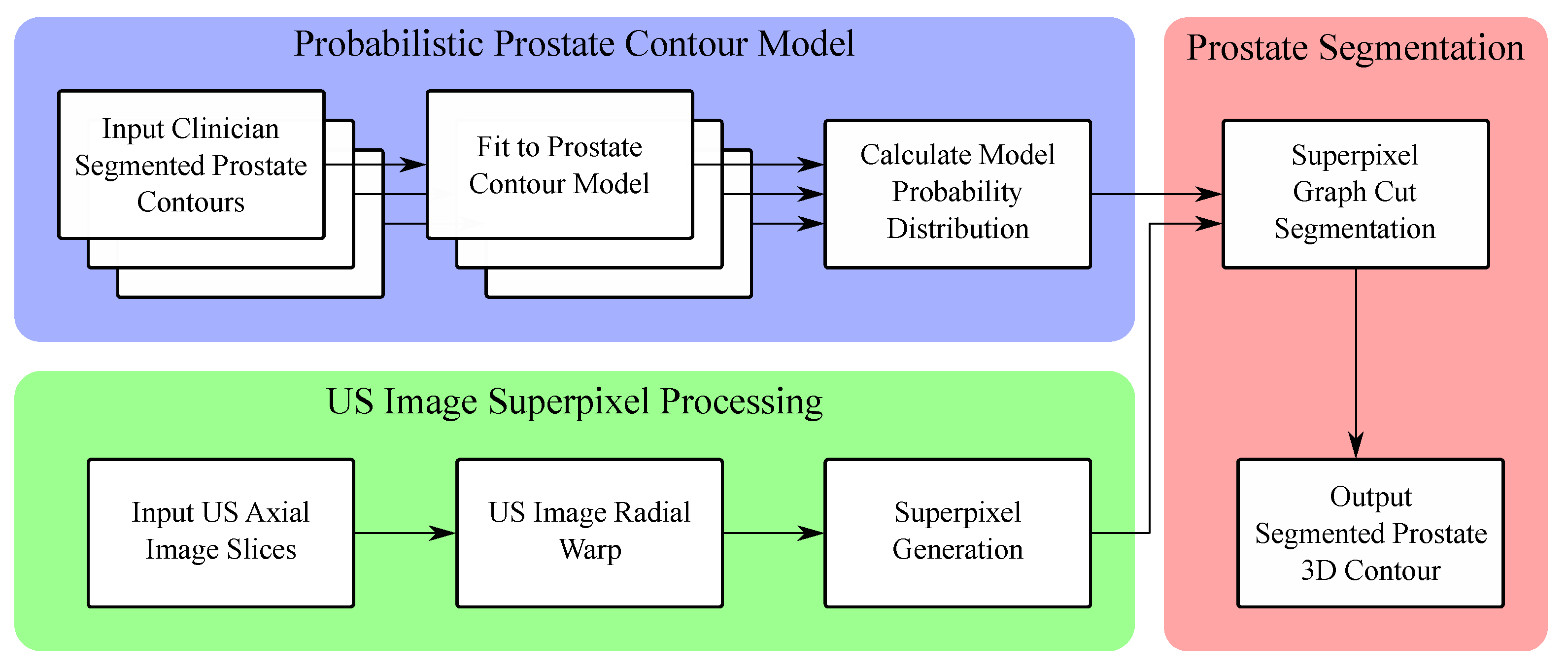
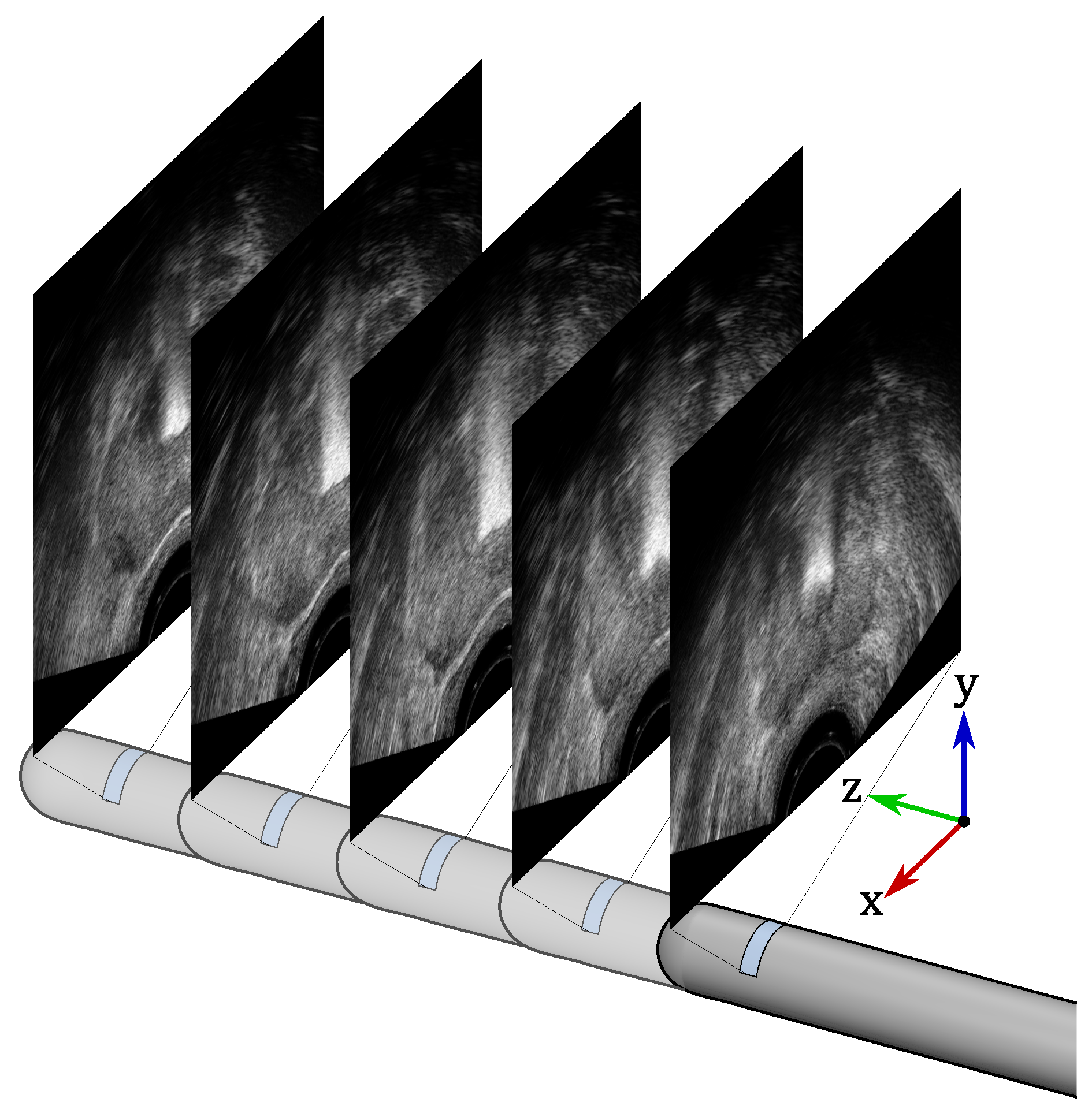
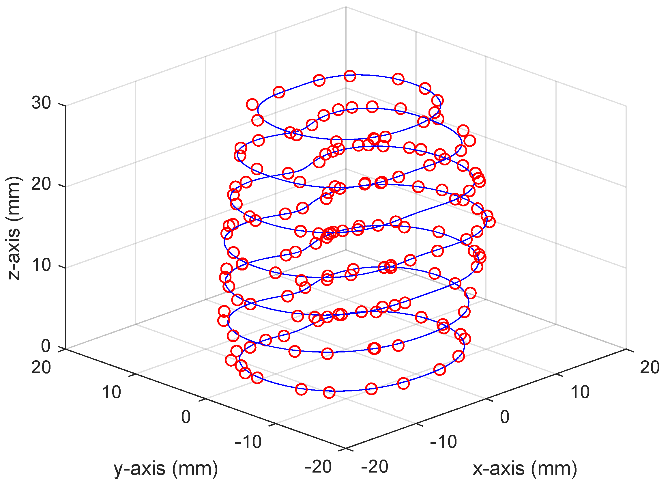
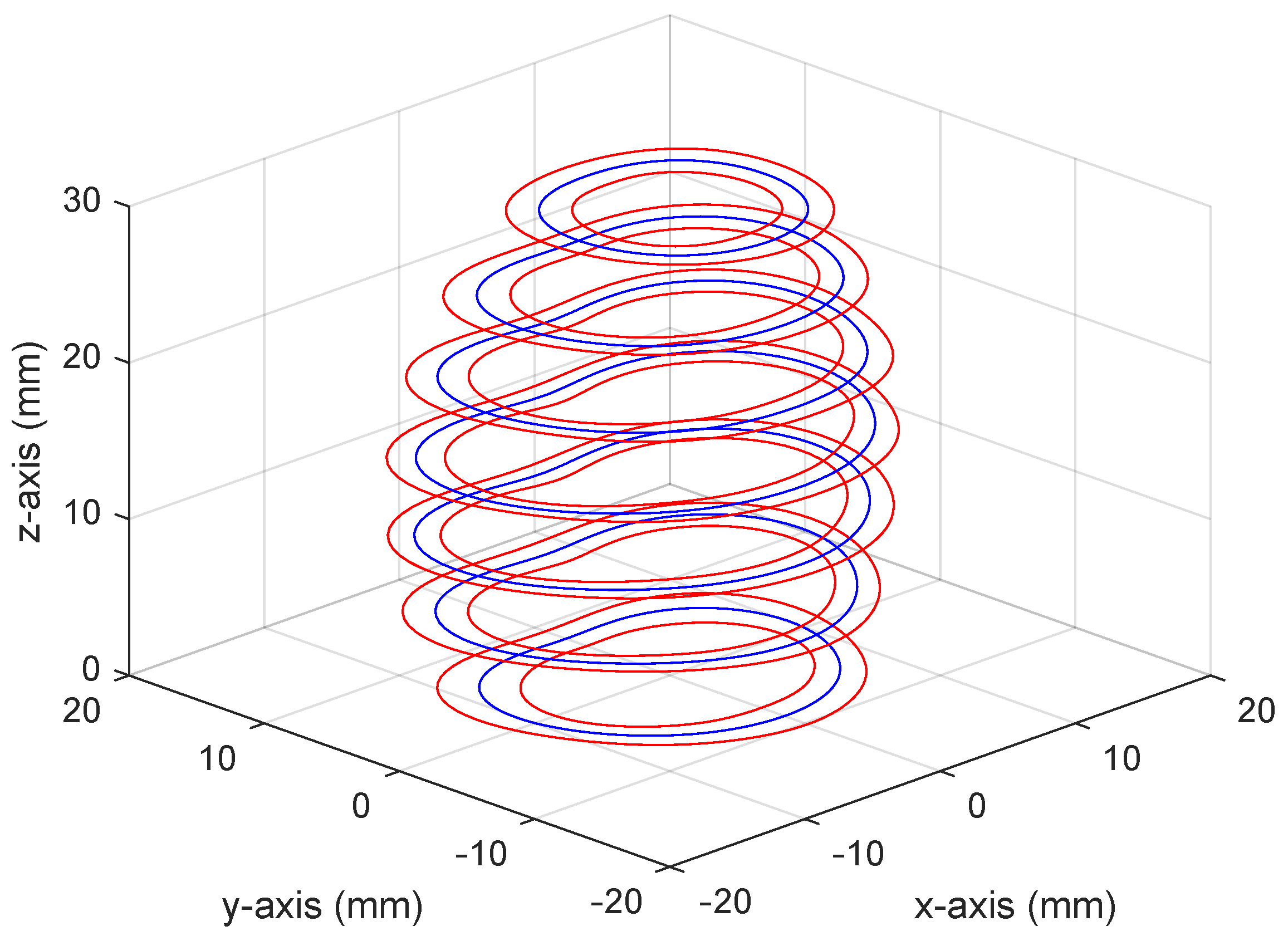
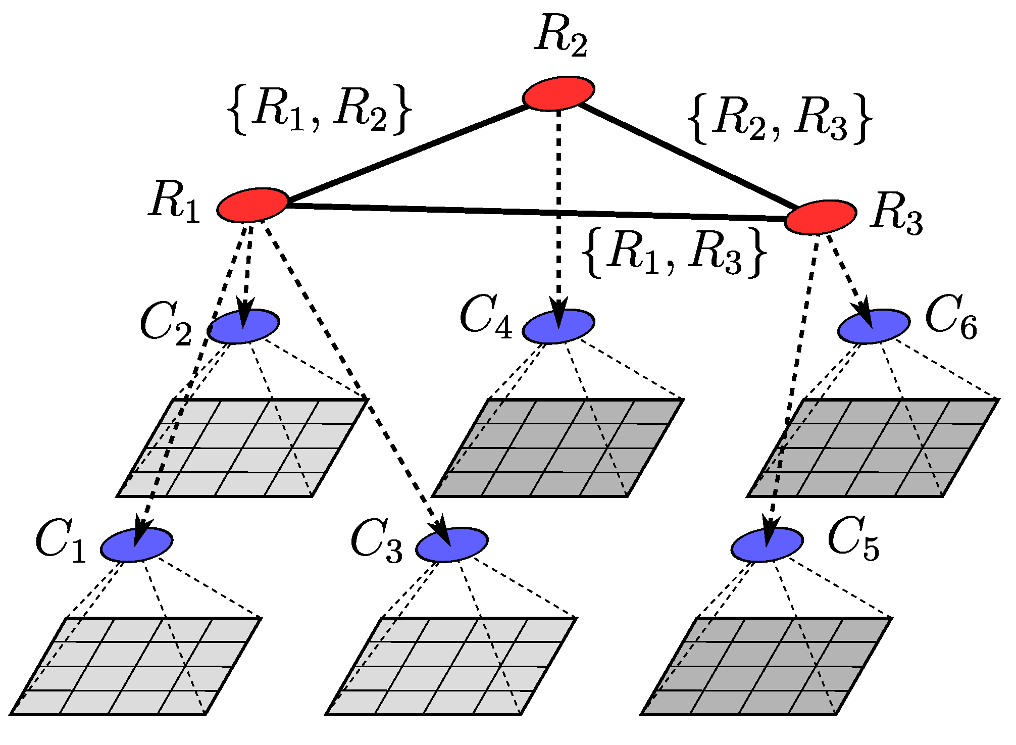
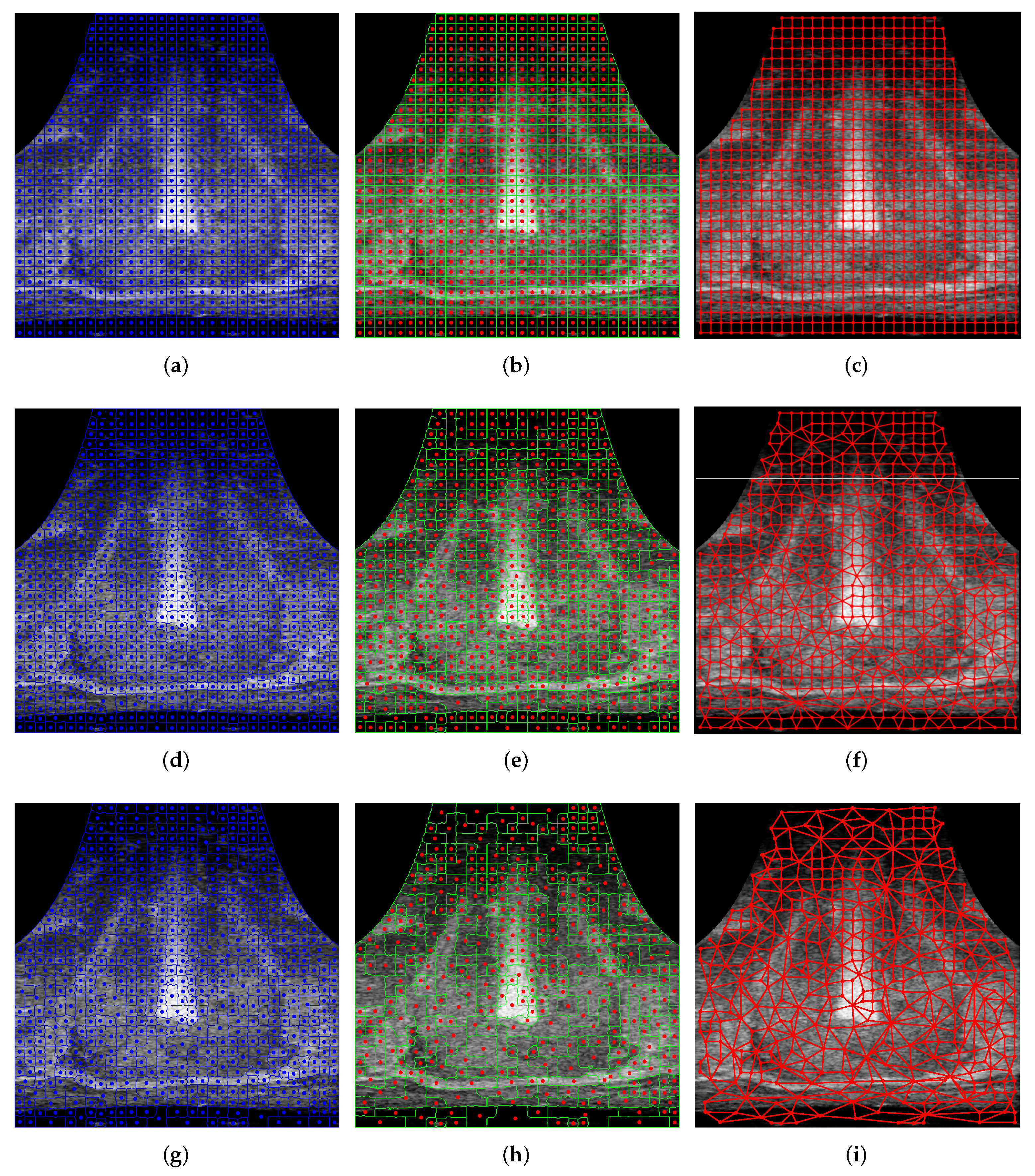
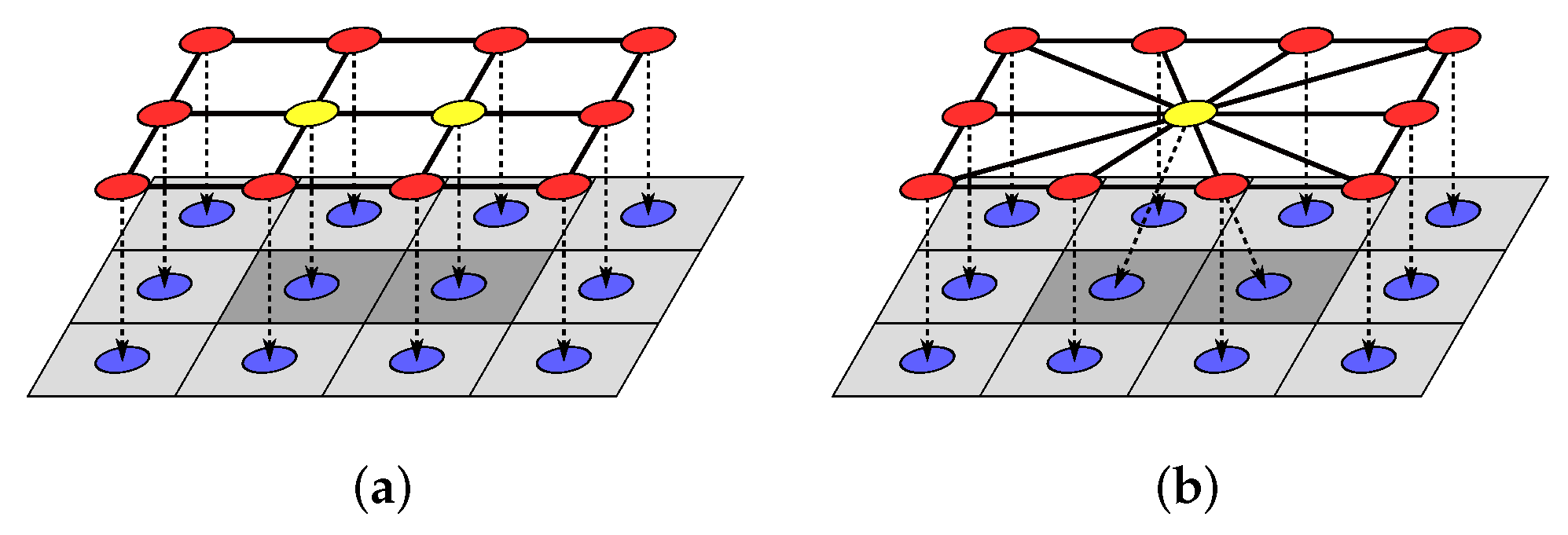
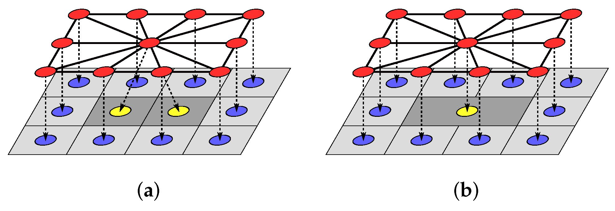
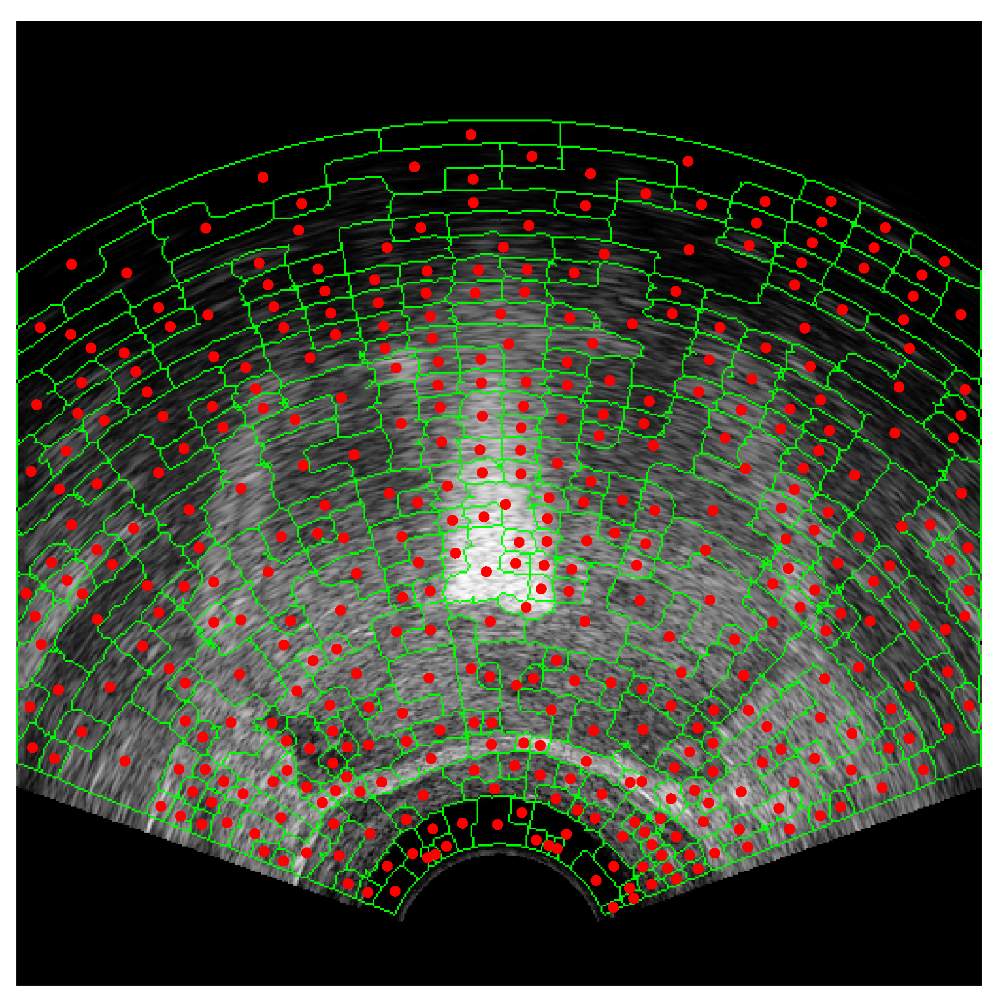
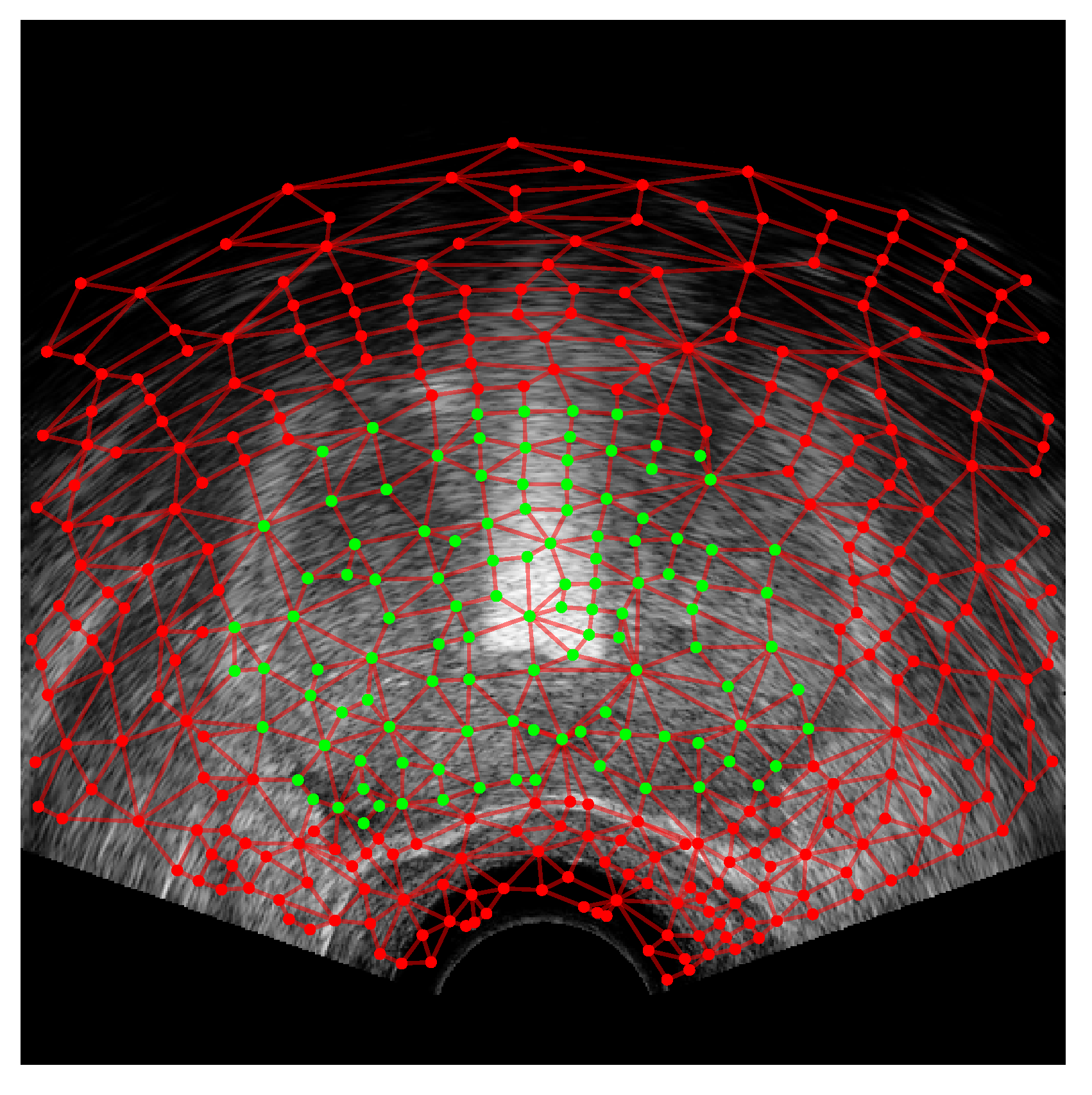
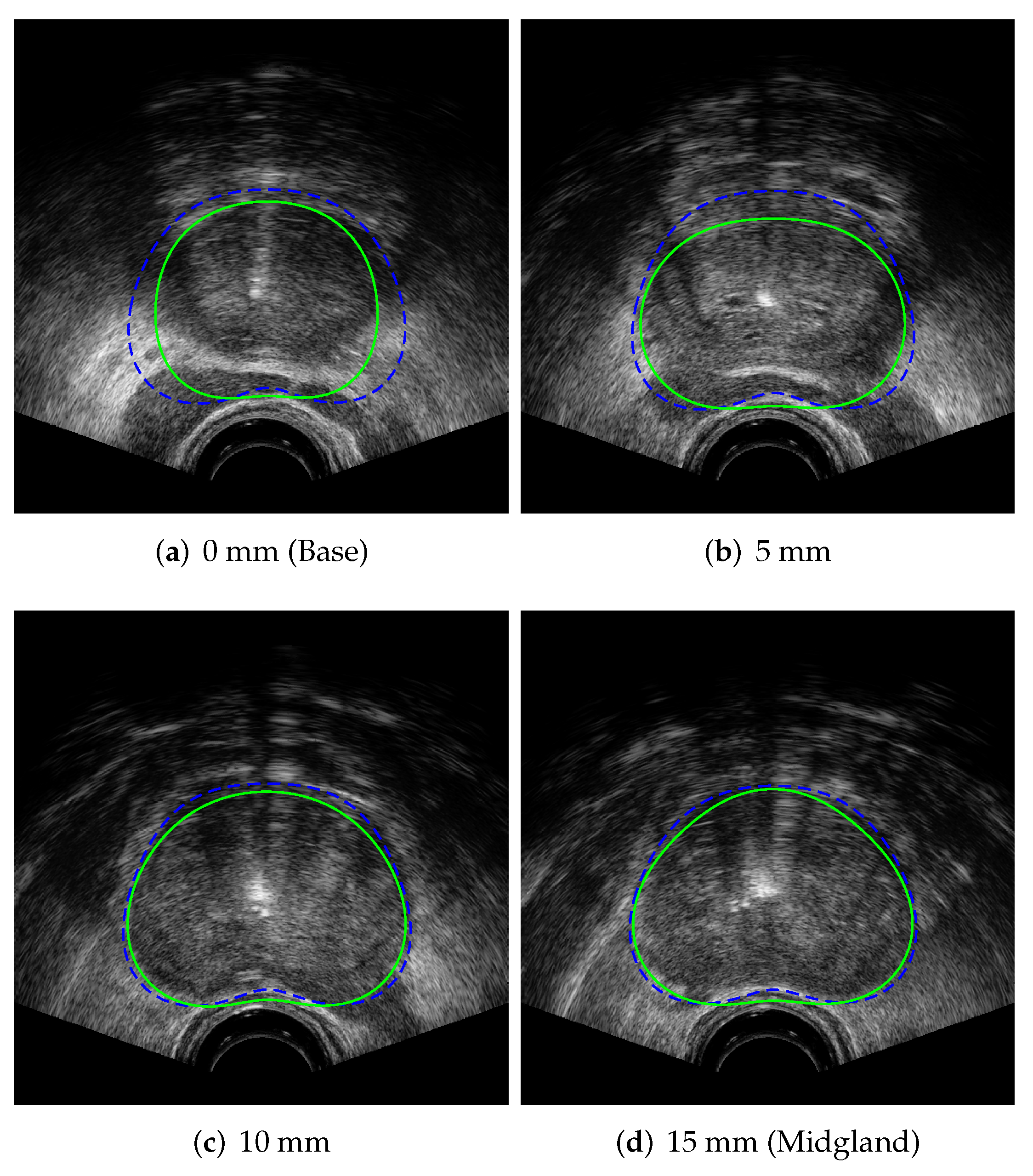
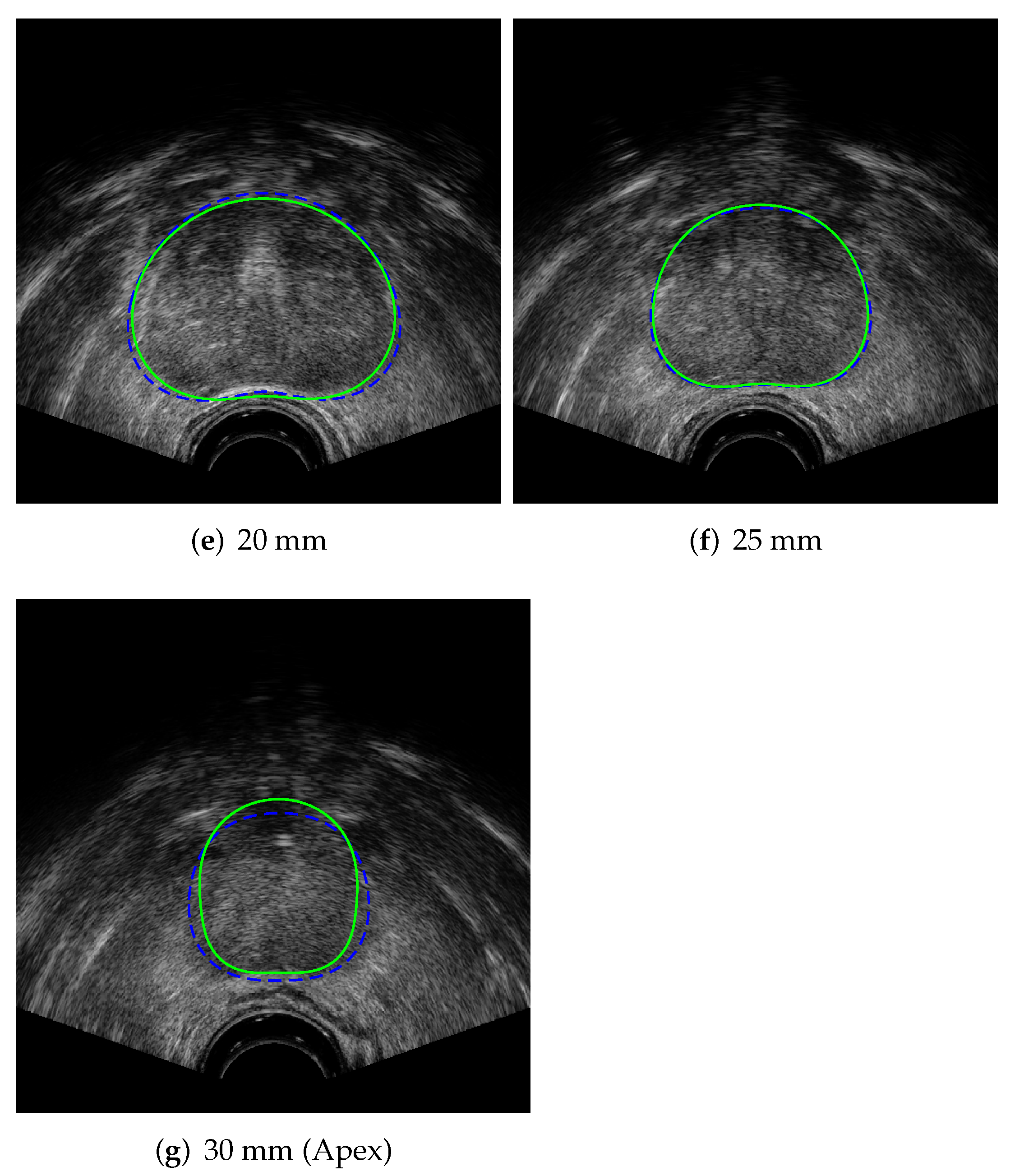
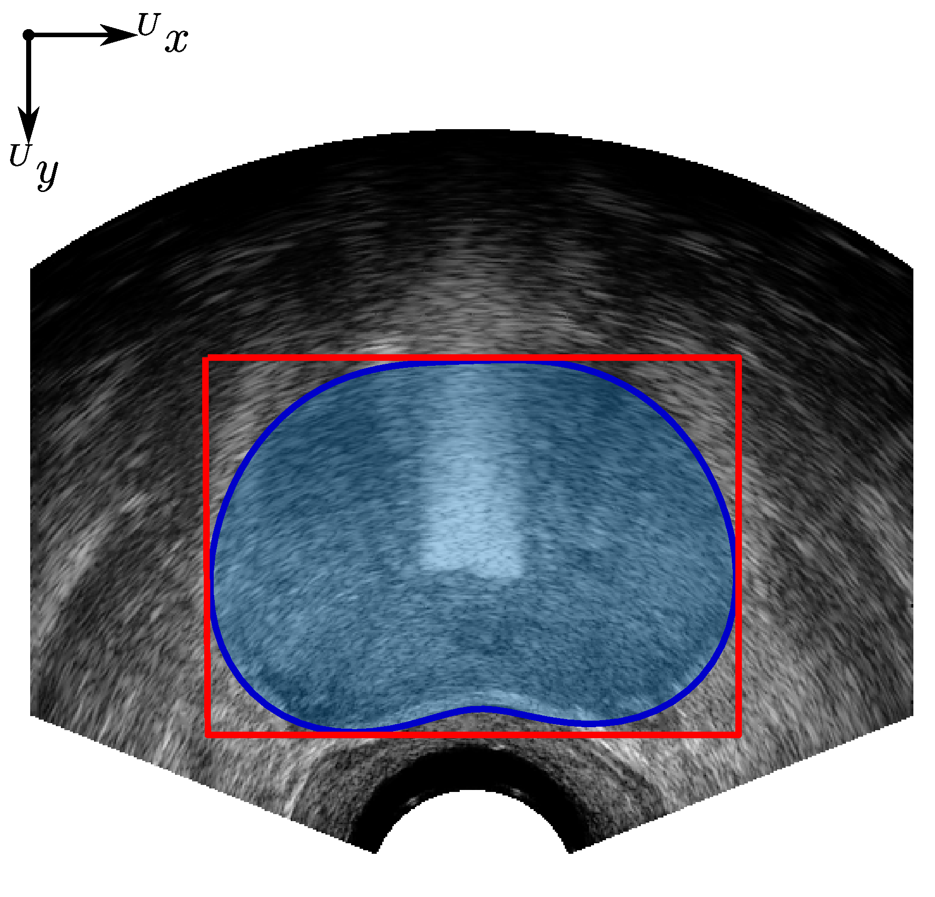
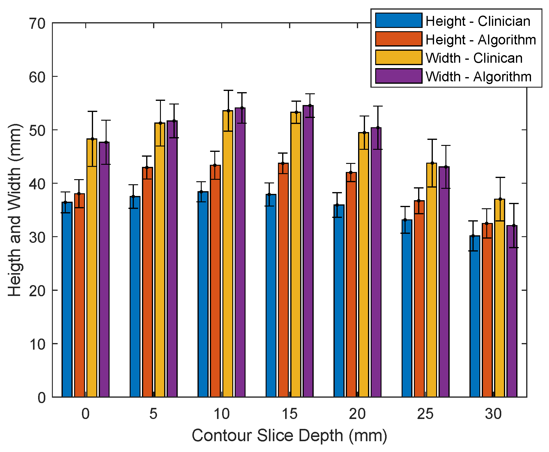
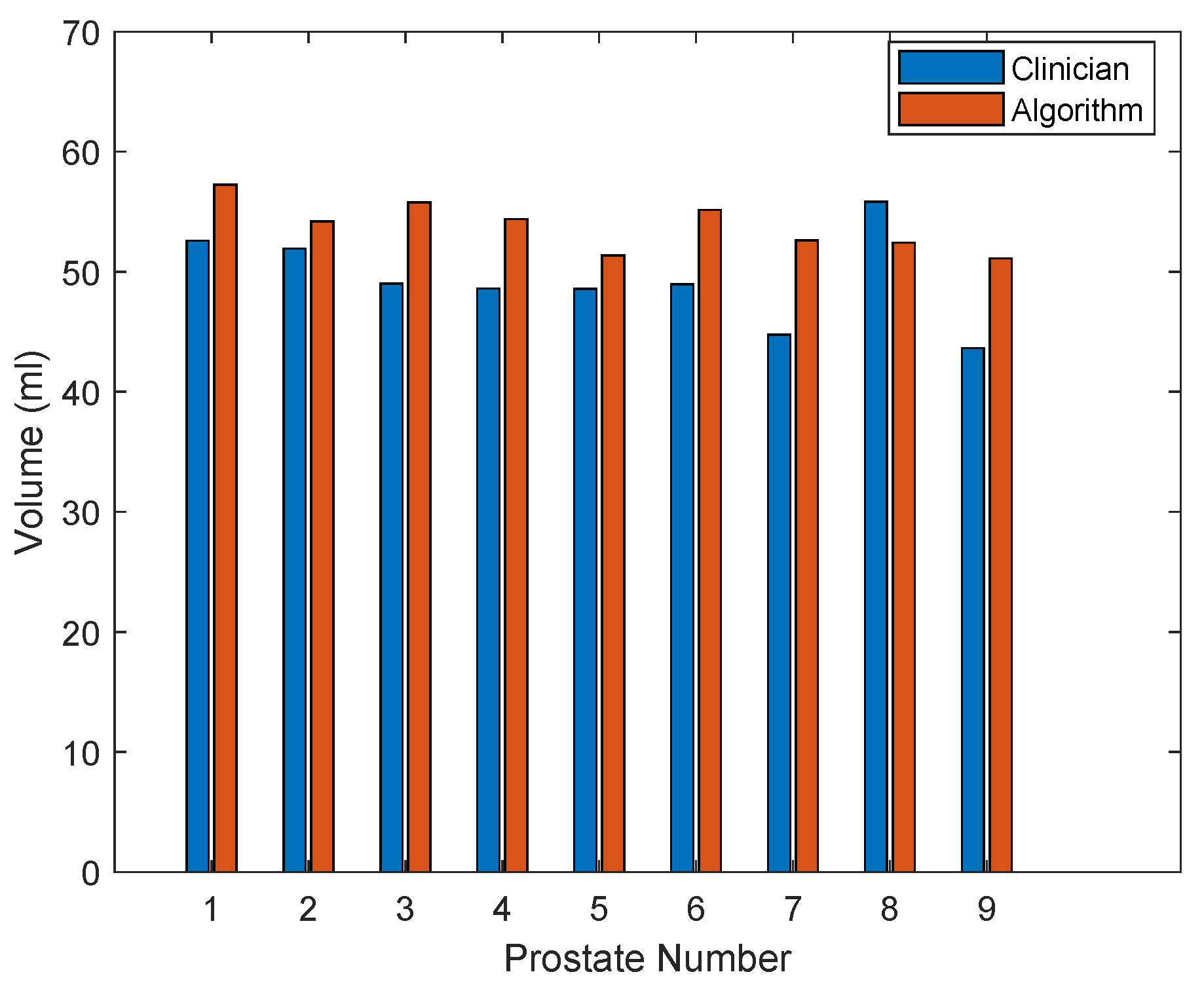
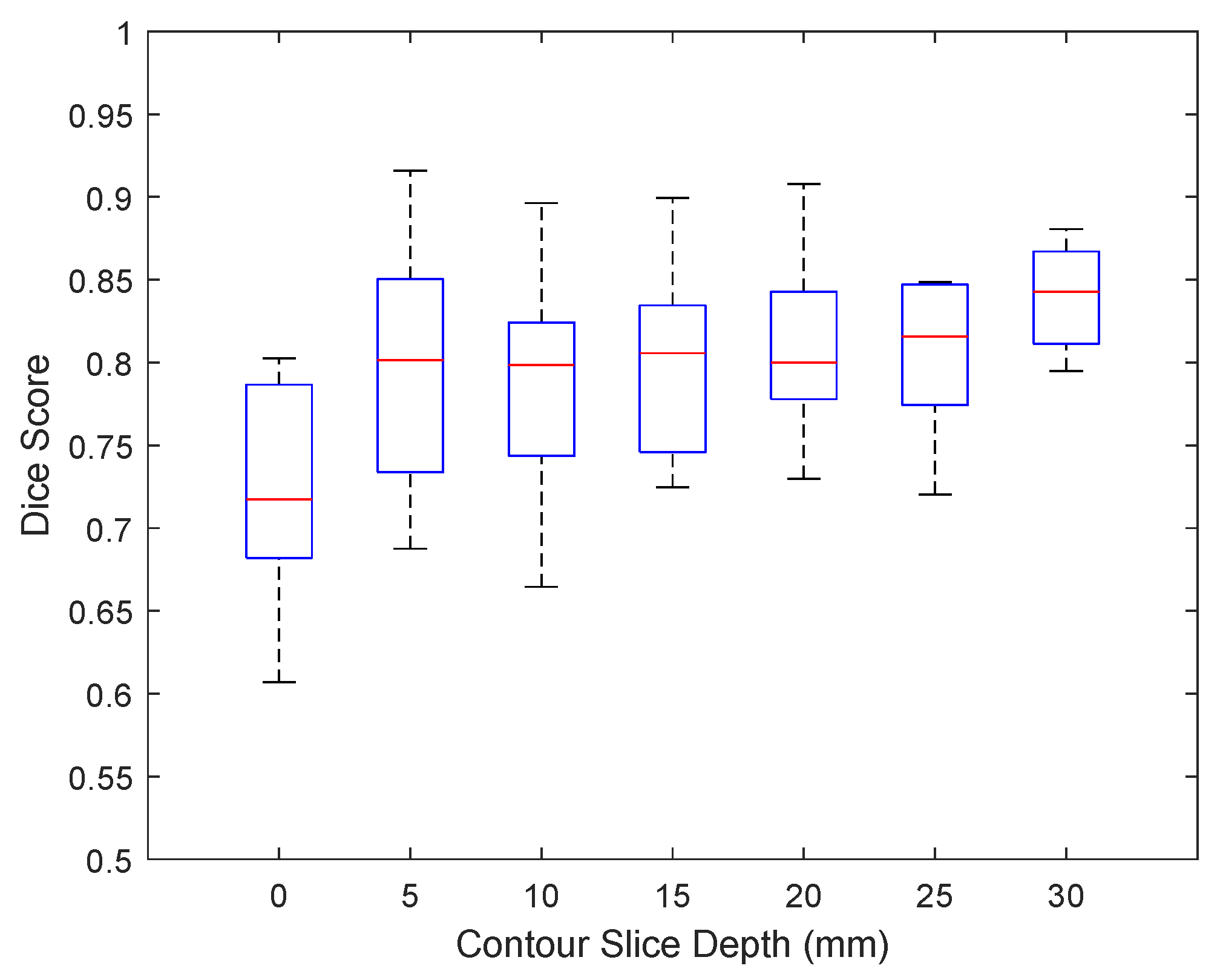
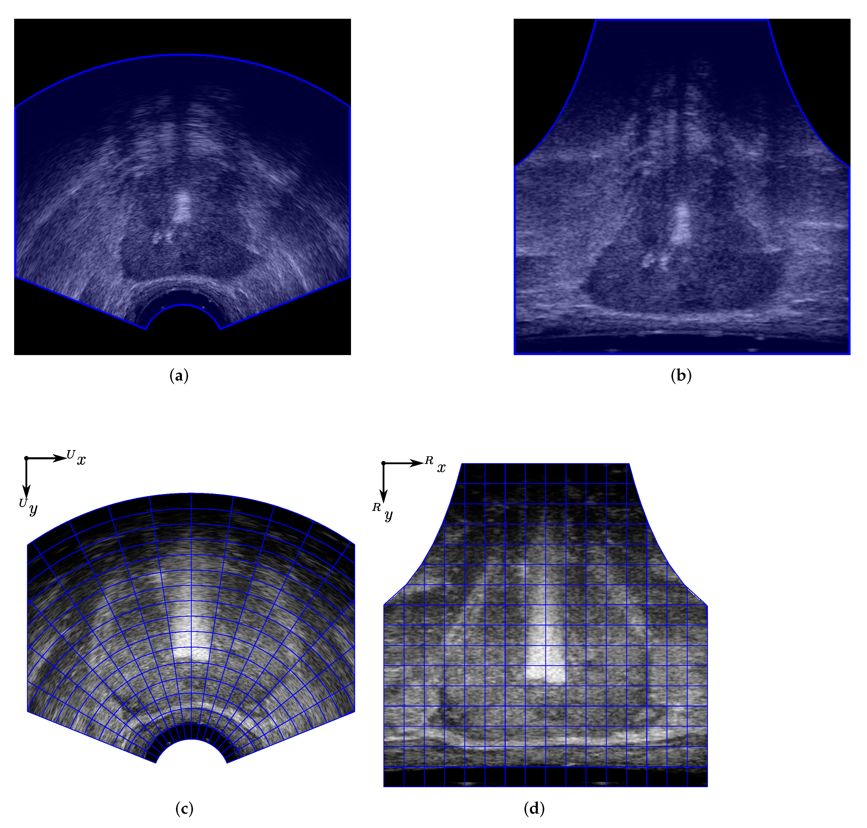
Table 1.
Prostate model fitting results.
| Data Set | Average MSE (mm) | Average Max Abs Error (mm) | Range of Max Abs Error (mm) |
|---|---|---|---|
| US Contours | 0.611 (±0.165) | 1.519 (±0.310) | 0.679–2.031 |
| MR Contours | 0.616 (±0.167) | 1.565 (±0.305) | 0.794–2.124 |
Table 2.
Prostate segmentation contour results.
| Dataset | Mean Absolute Difference (mm) | Max Absolute Difference (mm) | Volume Difference (mL) | Volume Difference |
|---|---|---|---|---|
| Prostate 1 | 2.01 (±1.30) | 5.89 | 4.65 | 8.85 |
| Prostate 2 | 1.87 (±1.29) | 6.91 | 2.27 | 4.37 |
| Prostate 3 | 3.03 (±2.21) | 8.50 | 6.75 | 13.77 |
| Prostate 4 | 2.54 (±1.48) | 6.00 | 5.77 | 11.88 |
| Prostate 5 | 2.46 (±1.60) | 6.82 | 2.80 | 5.76 |
| Prostate 6 | 2.24 (±1.43) | 6.70 | 6.20 | 12.68 |
| Prostate 7 | 3.08 (±2.06) | 8.82 | 7.86 | 17.56 |
| Prostate 8 | 2.73 (±1.71) | 8.90 | -3.39 | 6.07 |
| Prostate 9 | 2.76 (±1.65) | 6.20 | 7.47 | 17.11 |
| Average | 2.52 (±1.66) | 7.19 (±1.22) | 4.49 (±3.53) | 10.89 (±4.90) |
Table 3.
Prostate segmentation Jaccard index results.
| Dataset | Average Jaccard Index | Min Jaccard Index | Max Jaccard Index |
|---|---|---|---|
| Prostate 1 | 0.84 (±0.04) | 0.79 | 0.92 |
| Prostate 2 | 0.85 (±0.06) | 0.75 | 0.91 |
| Prostate 3 | 0.77 (±0.02) | 0.73 | 0.79 |
| Prostate 4 | 0.79 (±0.06) | 0.73 | 0.87 |
| Prostate 5 | 0.79 (±0.04) | 0.72 | 0.83 |
| Prostate 6 | 0.82 (±0.06) | 0.71 | 0.90 |
| Prostate 7 | 0.74 (±0.07) | 0.66 | 0.85 |
| Prostate 8 | 0.77 (±0.07) | 0.66 | 0.84 |
| Prostate 9 | 0.77 (±0.09) | 0.61 | 0.89 |
| Average | 0.79 (±0.07) | 0.71 (±0.05) | 0.87 (±0.04) |
Publisher’s Note: MDPI stays neutral with regard to jurisdictional claims in published maps and institutional affiliations. |
© 2022 by the authors. Licensee MDPI, Basel, Switzerland. This article is an open access article distributed under the terms and conditions of the Creative Commons Attribution (CC BY) license (https://creativecommons.org/licenses/by/4.0/).
Share and Cite
MDPI and ACS Style
Carriere, J.; Sloboda, R.; Usmani, N.; Tavakoli, M. Autonomous Prostate Segmentation in 2D B-Mode Ultrasound Images. Appl. Sci. 2022, 12, 2994. https://0-doi-org.brum.beds.ac.uk/10.3390/app12062994
AMA Style
Carriere J, Sloboda R, Usmani N, Tavakoli M. Autonomous Prostate Segmentation in 2D B-Mode Ultrasound Images. Applied Sciences. 2022; 12(6):2994. https://0-doi-org.brum.beds.ac.uk/10.3390/app12062994
Chicago/Turabian StyleCarriere, Jay, Ron Sloboda, Nawaid Usmani, and Mahdi Tavakoli. 2022. "Autonomous Prostate Segmentation in 2D B-Mode Ultrasound Images" Applied Sciences 12, no. 6: 2994. https://0-doi-org.brum.beds.ac.uk/10.3390/app12062994
Note that from the first issue of 2016, this journal uses article numbers instead of page numbers. See further details here.