TTCNN: A Breast Cancer Detection and Classification towards Computer-Aided Diagnosis Using Digital Mammography in Early Stages

Abstract

Breast cancer is a major research area in the medical image analysis field; it is a dangerous disease and a major cause of death among women. Early and accurate diagnosis of breast cancer based on digital mammograms can enhance disease detection accuracy. Medical imagery must be detected, segmented, and classified for computer-aided diagnosis (CAD) systems to help the radiologists for accurate diagnosis of breast lesions. Therefore, an accurate breast cancer detection and classification approach is proposed for screening of mammograms. In this paper, we present a deep learning system that can identify breast cancer in mammogram screening images using an “end-to-end” training strategy that efficiently uses mammography images for computer-aided breast cancer recognition in the early stages. First, the proposed approach implements the modified contrast enhancement method in order to refine the detail of edges from the source mammogram images. Next, the transferable texture convolutional neural network (TTCNN) is presented to enhance the performance of classification and the energy layer is integrated in this work to extract the texture features from the convolutional layer. The proposed approach consists of only three layers of convolution and one energy layer, rather than the pooling layer. In the third stage, we analyzed the performance of TTCNN based on deep features of convolutional neural network models (InceptionResNet-V2, Inception-V3, VGG-16, VGG-19, GoogLeNet, ResNet-18, ResNet-50, and ResNet-101). The deep features are extracted by determining the best layers which enhance the classification accuracy. In the fourth stage, by using the convolutional sparse image decomposition approach, all the extracted feature vectors are fused and, finally, the best features are selected by using the entropy controlled firefly method. The proposed approach employed on DDSM, INbreast, and MIAS datasets and attained the average accuracy of 97.49%. Our proposed transferable texture CNN-based method for classifying screening mammograms has outperformed prior methods. These findings demonstrate that automatic deep learning algorithms can be easily trained to achieve high accuracy in diverse mammography images, and can offer great potential to improve clinical tools to minimize false positive and false negative screening mammography results.

1. Introduction

Cancer is considered to be the gradual expansion and growth of abnormal cells in the human body. Breast cancer has been among the major cause of death among women worldwide [1,2]. Breast cancer has a higher death rate than any other disease, i.e., malaria or tuberculosis. The World Health Organization (WHO) cancer research institute (International agency for research on Cancer (IARC) and the American Cancer Society) reported that in 2018, there were 17.1 million cancer cases globally and it is expected to double by 2025 [3]. Although extensive research has been done by medical professionals and researchers, they cannot provide the best method of treating breast cancer to obtain the long-awaited treatment and guarantee the potential for reliable evidence for its prevention [4]. In addition, some important parts of cancerous tissue related to breast cancer are aggressive and pose the greatest threat to the lives of patients, because they are more likely to cause infections in other vital organs of the human body [5,6]. The enormous growth of the area of the mammary cells can cause tumors in women. Depending on the area, size, and location, these large tumor cells divide into cancer cells and non-cancer cells based on breast cancer reporting and data system (BI-RAD) scores [7,8]. Non-cancerous tumors are known as benign which is signified to the primary tumor area and the cancerous tumors are known as malignant and secondary tumor area. Benign tumors are treatable and their expansion can be restrained by taking the proper medications and will not endanger the lives of women [9,10]. Secondary tumors can spread to distant metastases or adjacent tissues. When cancer cells penetrate the lymphatic system or blood, malignant tumors can escalate to different parts of the body. The tumor stems from uncontrolled cell proliferation in the breast [11,12]. A malignant tumor can be treated only if the patient acquires appropriate treatment with surgery or radiation [13,14].

In the breast, cancer cells can increase to the lymph nodes and affect other body parts, i.e., lungs. Breast cancer usually begins with ductal dysfunction (invasive ductal carcinoma). Although, it can also originate in glandular tissues and other cells called lobules and breast tissue [15]. The researchers also found that changes in hormones, lifestyle, and the environment also increase the risk of breast cancer [16,17]. Low dose X-ray examination of the breast is utilized to envisage the internal structure of the breast. This process is medically called mammography. This is evaluated as the best suitable approach for the detection of breast cancer. Compared to previously used equipment, mammography shows the breast to a much lower radiation dose [18]. 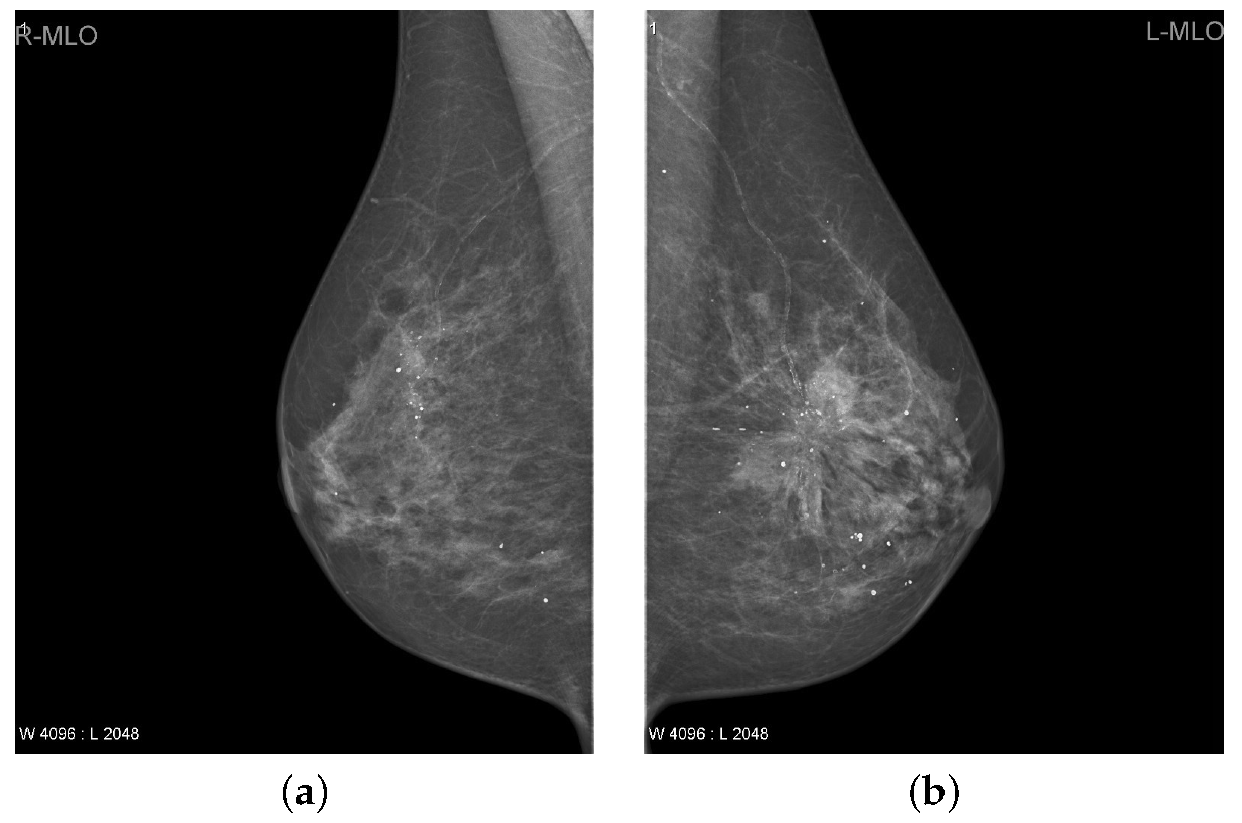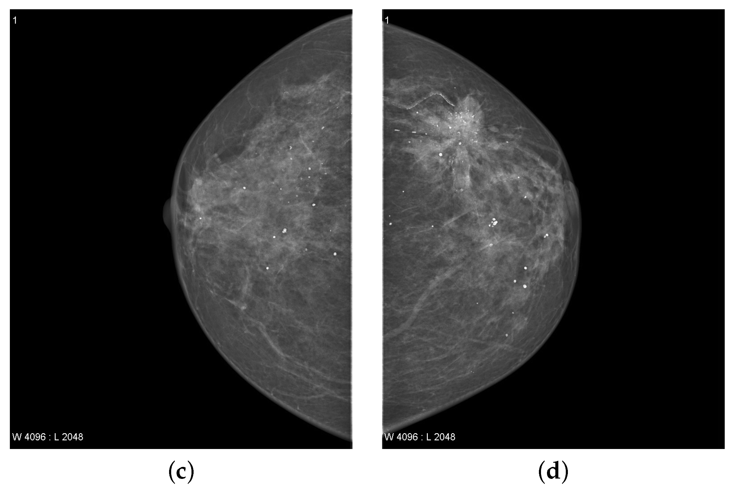It is one of the most reliable screening tools and has been shown to be a significant approach for early breast cancer detection in recent times [19]. A mammogram of each breast was recorded in two different views, namely the medial-lateral oblique (MLO) view and the cranio-caudal (CC) view as shown in Figure 1. Estimated new cases recorded in 2021 were 281,550 and the percentage of all the new cancer cases was 14.8% in the U.S. The estimated deaths in 2021 was around 43,600 having a percentage of 7.2%. The 5-year relative survival rate of breast cancer from 2014 to 2019 was 92.16% in the U.S [20].

Many researchers focus on biomedical imaging to assist specialist radiologists. Early detection of tumors has a significant role in the diagnosis and analysis of breast cancer. Detection of breast cancer malignancies in early stages is important. Various biomedical imaging methods have been utilized to determine breast cancer, i.e., magnetic resonance imaging (MRI), ultrasound, and mammography [22]. Owing to the huge number of images,  radiologists face many problems identifying suspicious areas or cancer. Therefore, to reduce the load, an efficient automated method is required to help radiologists significantly. A computer-aided diagnostic (CAD) model is used to assist radiologists detect malignant breast cancer tumors [23,24].

Recently, some research based on deep learning methods has addressed the concept of medical imaging on automated CAD systems [8,25,26,27,28,29,30]. In fact, deep learning approaches are the best option for medical image recognition and classification. A CAD system based on deep learning requires three successive phases: the pre-processing, parameters initialization, extraction of deep features and diagnosis [8,25]. Deep learning methods can be utilized to directly derive the large low–high levels deep hierarchical feature maps from the identical source breast image (mammogram) [8]. This shows that deep learning is the most efficient and dependable medical imaging method [8,25,31]. Recently, several CAD systems based on deep learning have been introduced to detect the breast lesions and are superior to traditional systems [32,33]. Automated detection of the breast lesions is the main task for the automatic evolution of CAD approaches to improve the diagnosis of breast cancer [8]. Accurate diagnosis of skeptical breast lesions plays an important part in obtaining a high true positive rate and enhancing the breast cancer final diagnosis [8,26]. Detecting breast lesions is a difficult task because these lesions are so diverse in shape, texture, size, and position. The use of image processing and deep learning methods to detect the breast lesions using traditional methods are proposed in [11,26]. Traditional technology relies on low-level manual functions and does not yet have the ability to perform identification tasks automatically [25]. Low contrast of mammogram images and detecting asymptomatic breast cancer through mammography is a difficult image classification task from the view of machine learning (ML) because the tumor itself only makes up a small part of the complete breast image. Recently, numerous new approaches based on deep learning recognition have been introduced to solve the problem of poor diagnosis performance of CAD approaches [8,31]. Classification of breast lesions is the last phase in the CAD model. The aim of this stage is to identify breast lesions that are considered benign or malignant [25,34]. The importance of the method of classification of breast lesions leans on the validity of the hypothetical characteristics which indicate the leading characteristics [8]. Deep features must have an appropriate feature distribution in order to identify the malignant and benign breast lesions [8,9].

The existing breast cancer detection system is time consuming, expensive, and requires additional work to operate the equipment for radiologists. From an image processing perspective, accurate and automatic detection of breast cancer is not easy. Hence, it is deemed a requisite to diagnose breast cancer at an early stage and treated properly. However, breast cancer detection requires proper screening system and automation because of the following reasons [5]:

• False diagnosis and prediction.
• The tumor appears in an area with significantly lower contrast.
• Lack of reliability of human experience in diagnosis.
• Overload of the radiologists.
• High complexity of memory.
• Degree of human inaccuracy in diagnosis.
• Current deep learning algorithms need large amounts of training data to overcome the problems of overfitting.
• Existing breast cancer detection methods are computationally complex and require more treatment time to identify accurate tumors.

In addition, manual breast cancer diagnosis can take months and the localized stage of cancer infection can progress to a critical stage where survival cannot be achieved. Therefore, an accurate automated breast cancer detection method is required to diagnose cancer [35]. Today, deep learning approaches have been introduced for breast lesion detection and classification to enhance their accuracy, and have become an important element of CAD systems. The CAD techniques based on image processing are becoming more popular to accelerate the work of doctors for breast cancer diagnosis and reduce diagnosis time [8,36]. The proposed TTCNN system is effectual for early detection of breast cancer, however, the proposed system is effective for all stages of cancer. Detecting the small tumor in a whole breast is a more difficult task as compared to detecting the large area of tumor at a later stage. To this end, we propose a new approach of early breast cancer detection, which has the following contributions.

• As a pre-processing step, a modified contrast-limited adaptive histogram equalization (CLAHE) algorithm is utilized to refine the edge details of the source image.
• We propose a new transferable texture convolutional neural network (TTCNN) for the classification of breast cancer.
• We use the energy layer (EL) in the proposed TTCNN framework. This allows us to preserve texture information, limit the size of the output vector, and refine the model’s overall learning ability.
• We perform the detailed functions of the most advanced CNN model for breast cancer classification i.e., InceptionResNet-V2, Inception-V3, VGG-16, VGG-19, GoogLeNet, ResNet-18, ResNet-50, and ResNet-101.
• A convolutional sparse image decomposition approach is implemented for the feature fusion and entropy controlled firefly approach is employed to optimize the feature selection.
• Aiming to check the stability of the proposed system, a comprehensive statistical analysis and comparison with the latest algorithms is performed.
• The proposed approach minimizes the time required for radiologists to diagnose cancer while assuring reliable accuracy of detection. The proposed approach takes less processing time and provides accurate results.

The rest of the article is structured as follows: Section 2 briefly expresses the literature review involved in the detection and classification of breast cancer. The detailed methodology of the proposed system is presented in Section 3. Section 4 analyzes the proposed approach performance in comparison with other modern approaches. Finally, we conclude this work with the direction of future research in Section 5.

2. Related Work

Modern medical procedures actively use mammography images for breast cancer diagnosis [37]. This section systematically reviews the esteem achievement and performance on breast cancer detection and classification.

Over the past few years, deep learning methods in the field of image recognition, segmentation, detection, and computer vision have received much attention and interest [8,28,38]. In fact, deep learning has been utilized to address the inadequacies of traditional CAD approaches [8]. This is because conventional CAD approaches are based on manually developed functions and have limited diagnostic accuracy [35]. The similarity between benign and malignant lesions and their enormous changes in size, shape, color, and texture have challenged traditional methods [19,25]. CAD approaches have demonstrated the ability to use deep learning to discover complex hierarchical deep features automatically to improve diagnostic operation [8,32,35]. Many CAD approaches use conventional image processing and deep learning methods, but the use of deep learning detection and classification in breast imaging is inadequate for breast lesion diagnosis.

In recent years, AlexNet [39], ResNet [40], VGG16 [41], Inception [42], GoogleNet [43], DenseNet [44] deep learning models provide improve performance of classification as compared to the shallower ones. The overall classification accuracy of VGG16, ResNet50, and Inception-V3 reached 95%, 92.5%, and 95.5% respectively. The performance of classification of these deep learning methods is much better than that of the shallow model, but manually detection and memory complexity during training still remain challenges.

Several scholars have worked on the automatic detection and classification of breast cancer aiming to enhance the accuracy. For example, Al-antari et al. [4] evaluated the use of the YOLO detector to perceive breast injury from mammograms. Three deep learning classifiers, i.e., Inception ResNet-V2, ResNet-50, and feedforward CNN are used to assess classification of breast lesions using a digital database for screening mammography (DDSM) and the INbreast database. With these classifiers, the method acquired an accuracy rate of 95.32%. Al-antari et al. [8] used a CAD model (four-fold cross-validation) to estimate a full resolution convolutional network (FrCN) with X-ray mammograms using INbreast dataset. This approach achieved an accuracy of 95.96%, F1 score of 99.24%, and matthews correlation coefficient of 98.96%.

Chouhan et al. [19] proposed a diverse features (DFeBCD) method for breast cancer detection to classify mammograms as normal or abnormal. The IRMA mammography dataset uses two classifiers, a support vector machine (SVM) and an emotion learning-inspired integrated classifier (ELiEC). The ELiE classifier performance is superior to SVM and the accuracy rate reaches 80.30%. Muduli et al. [45] used the lifting wavelet transform (LWT) to obtain the region of interest features from the breast images. The size of the feature vectors diminish using a fusion of principal component analysis (PCA) and linear discriminant analysis (LDA) approaches. The extreme learning machine (ELM) and moth flame optimization approach is used for the classification using the DDSM and mammographic image analysis society (MIAS) databases. This approach attained an accuracy of 98.76% and 95.80% for DDSM and MIAS databases respectively. Junior et al. [46] presented a breast cancer method based on diversity analysis, geostatistics and alpha form using the SVM classifier on DDSM and MIAS datasets and achieved the detection accuracy of 96.30%. Ghosh et al. [47] presented an algorithm for segmentation utilizing intuitionistic fuzzy soft set and multigranulation rough set. The intuitionistic fuzzy soft set takes information from input images through various fuzzy membership operations. This approach deals with ambiguity between damaged and undamaged pixels when forming the membership function. This reduces the distant pixels that are not in the region of interest, the diseased tissue in the mammogram is separated by a rough approximation of the fuzzy concept of the multiregional granulation space. Zheng et al. [48] developed an efficient adaboost deep learning method for the recognition of breast cancer. This work focused on the combination of various deep learning approaches with feature extraction and selection using classification and segmentation methods to evaluate the result and focus on finding the most suitable method and obtained an accuracy of 97.2%.

Harefa et al. [49] utilized the gray level co-occurrence matrix (GLCM) and SVM classifier to detect breast cancer abnormalities on the MIAS database and achieved an accuracy of 93.88% and outperformed k-Nearest Neighbour (kNN). Samala et al. [50] presented a use of the deep neural network for multilevel transfer learning for digital breast tomosynthesis. ImageNet knowledge first records mammogram information and then optimizes it during multi-step transmission of digital breast tomosynthesis information. Then the freezing of most of the convolution neural network (CNN) framework was compared to two transmission systems with the first convolution layer. Qi et al. [51] proposed a deep active learning approach for the classification of breast cancer with the aim of maximizing the precision of learning with very limited labels. This approach manually annotates the most valuable unlabeled samples and integrates them into the training set. Then update the system repeatedly as the training set grows. Two deep active learning framework selection strategies are proposed i.e., confidence boosting strategy and an entropy based strategy on the breast cancer histopathological (BreakHis) database. This approach reduced the cost of annotation by up to 66.67%, which is more accurate than the standard query strategy. Agarwal et al. [52] developed a patch-based CNN algorithm for the identification of lesions in breast in the full-field digital mammograms (FFDM) using a pre-trained CNN models (VGG16, ResNet50, and InceptionV3) for the extraction of features and attained the results of detection with a true positive rate (TPR) of 98%.

Irfan et al. [53] developed an algorithm based on dilated semantic segmentation network (DICNN) with morphological operation. A DenseNet201 is used for the feature extraction. The feature vectors acquired from DenseNet201 and 24 layer CNN employing parallel fusion were fused to categorize the nodules. These feature vectors are merged with the SVM classification and attained an accuracy of 98.9%. Rajinikanth et al. [54] developed a breast cancer detection method using breast thermal images. The two image features GLCM and local binary pattern (LBP) with heterogeneous weights are used to classify the breast thermal images into healthy and DCIS class by using the SVM and decision tree (DT) classifier. This algorithm had an accuracy of 92%. Kadry et al. [55] presented a joint thresholding (slime mould method and Shannon’s entropy) and watershed segmentation method to improve and obtain the breast tumor from 2D MRI slices. The extracted breast tumor and ground truth image is executed and the essential image performance values (IPV) are calculated. Some of the existing works with dataset information and results are illustrated in

Table 1. Detailed summary of recent related works on breast cancer detection and classification.

References	Approach and Methods Used	Modality	Dataset	Results
Al-antari et al. [4]	YOLO detector, Inception ResNet-V2, ResNet-50, and feedforward CNN	Mammography	DDSM, INbreast	Accuracy = 95.32%
Al-antari et al. [8]	Full Resolution Convolutional Network (FrCN)	Mammography	INbreast	Accuracy = 95.96%
Chouhan et al. [19]	Diverse Features (DFeBCD), SVM, and ELiEC	Mammography	IRMA	Accuracy = 80.30%
Muduli et al. [45]	Lifting Wavelet Transform (LWT)	Mammography	DDSM, MIAS	Accuracy = 98.76% and 95.80%
Junior et al. [46]	Diversity Analysis, Geostatistics, and Alpha Form	Mammography	DDSM, MIAS	Accuracy = 96.30%
Ghosh et al. [47]	Intuitionistic fuzzy soft and Multigranulation rough set	Mammography	MIAS, MedPix	Accuracy = 87.22%
Zheng et al. [48]	Efficient Adaboost	Mammography	ACRIN	Accuracy = 97.2%
Harefa et al. [49]	GLCM and SVM	Mammography	MIAS	Accuracy = 93.88%
Samala et al. [50]	Multi-stage transfer learning	Mammography	DDSM	AUC = 0.92
Qi et al. [51]	Deep active learning	Histopathology	BreaKHis	-
Agarwal et al. [52]	Patch-based CNN	Mammography	DDSM, INbreast	TPR = 0.93
Rajinikanth et al. [54]	GLCM and LBP	Thermography	DITI-India	Accuracy = 92%

.

From literature research, previous breast cancer detection and classification approaches have led to better information extraction. However, there are still numerous problems that require serious attention, i.e., (i) the tumor appears in a location with significantly lower contrast, (ii) memory complexity is high, (iii) existing approaches are computationally complex and require more treatment time to identify the accurate tumor, (iv) current deep learning approaches require a large amount of training data to overcome the problems of overfitting and high computational cost, and (v) practical implementation.

To resolve the above mentioned problems, we have proposed a new breast cancer detection and classification approach. This will be discussed in more detail in the next section.

3. The Proposed Transferable Texture Convolutional Neural Network (TTCNN) Method

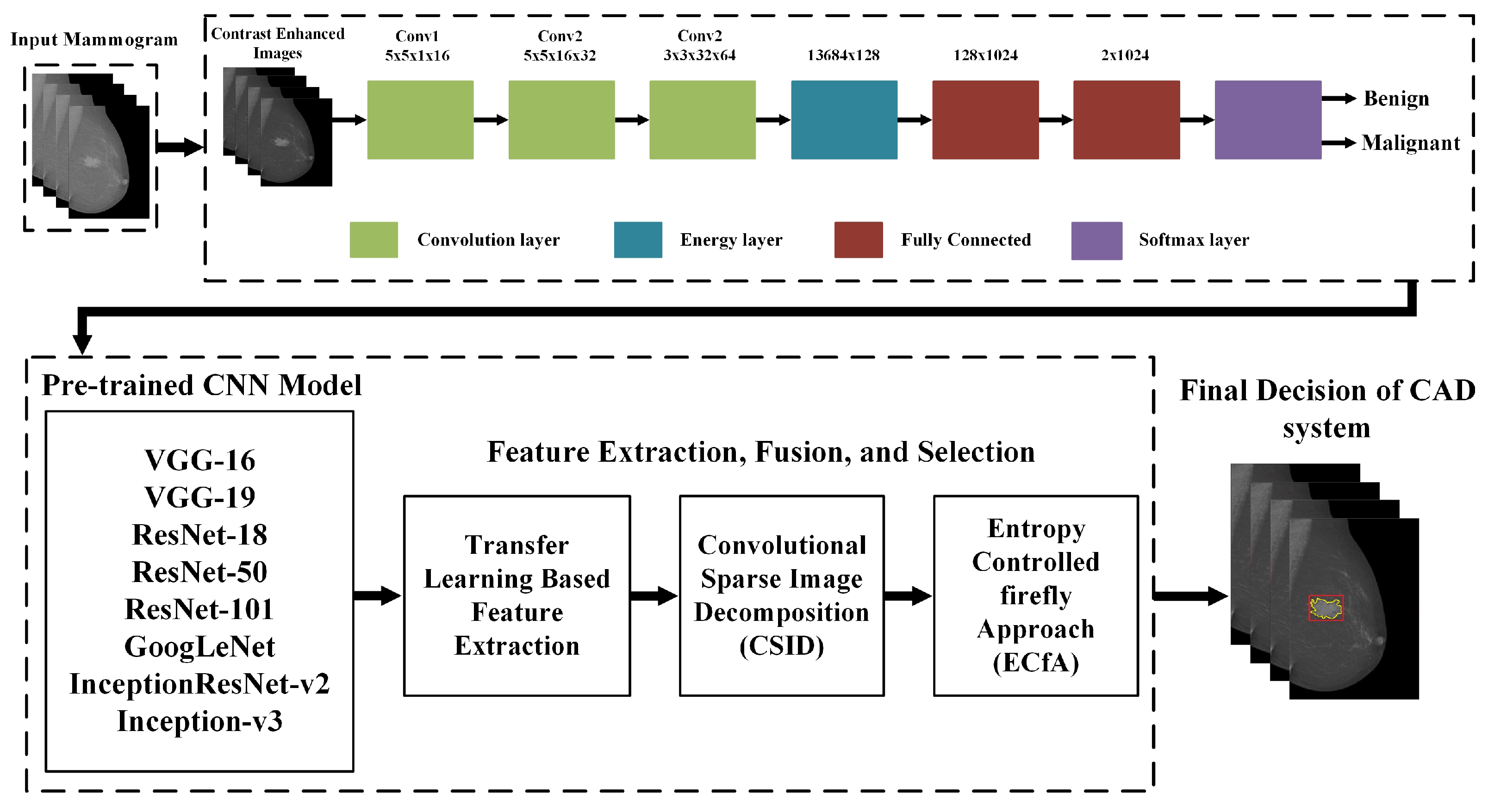
In this paper, a deep learning based Transferable Texture Convolutional Neural Network (TTCNN) method is proposed for breast cancer diagnosis and classification using digital X-ray mammograms. Firstly, a pre-processing approach is executed for contrast enhancement on the source image to improve the contrast. After that, the proposed TTCNN is applied on the pre-processed images for breast cancer malignant and benign classification. The proposed TTCNN classification then perform on the latest deep features from the deep convolutional neural network (DCNN) models, i.e., InceptionResNet-V2, Inception-V3, GoogLeNet, VGG-16, VGG-19, ResNet-18, ResNet-50, and ResNet-101 for the feature extraction and executes transfer learning to redeem the selected databases. The proposed method contains six phases that include the materials and methods, contrast enhancement, proposed TTCNN architecture, transfer learning based deep feature extraction, feature fusion and the feature selection. These steps are elaborated in the following subsections. A schematic diagram of the proposed approach is presented in Figure 2.

3.1. Materials and Methods

3.1.1. Dataset

This work used three digital breast X-ray databases to assess the proposed CAD approach. The datasets are DDSM [56], INbreast [57] and MIAS [58].

DDSM

The DDSM database was compiled by a team of experts from the University of South Florida [56]. The DDSM dataset consists of digitized images in joint photographic experts group (jpeg) format compressed scanned mammography film. In this work, we have used CBIS-DDSM (Curated Breast Imaging Subset of DDSM) which is a modernized version of DDSM decompressed in DICOM format. The DDSM database includes 2620 breast cases divided into 43 different volumes. In each case, each breast uses two different slide views (MLO and CC) to collect four mammograms [7]. The average size of a DDSM database is 3000 × 4800 pixels [4]. This contains the cancer type (benign or malignant) and the location of the wound [56]. Mammograms in the DDSM dataset are categorized in three sets i.e., normal, benign, and malignant by experts based on the BI-RAD score [7]. The CBIS-DDSM database consists of pixel-by-pixel annotations for regions of interest (ROI), i.e., tumor, calcification and disease pathology (benign or malignant). Additionally, each ROI is marked as calcification or mass. Most mammograms consist of only one ROI. The motive of this work is to anticipate the benign and malignant state of each image.

INbreast

The INbreast database consists of digital mammograms and was obtained from the Portuguese University Hospital (Centro Hospitalar de S. Joao [CHSJ], Breast Centre, Porto) with the consent of the National Data Protection Commission of Portugal and Hospital’s Ethics Committee [57]. The average size of an INbreast database is 3328 × 4084 pixels. A total of 115 cases or patients were taken from INbreast dataset using both breast views (MLO and CC). In the 90 affected cases of both breasts (i.e., 360 mammograms), each person had 4 mammograms, but in the other 25 mastectomy patients (i.e., 50 mammograms) in only two mammograms were performed [57]. Therefore, a total of 410 mammograms were generated with MLO and CC images from 115 patients. This includes normal, benign and malignant cases [57]. All mammograms with breast lesions (107 cases in a total) were used for evaluation from both the MLO and the CC perspectives. Multiple mammograms showed various lesions and the BI-RAD score was used to classify a total of 112 breast lesions. Therefore, by using the BI-RAD 36 mammograms were collected to indicate benign cases and 76 mammograms were collected to explain malignant cases using BI-RAD. This dataset consists of pixel-level batch annotations and histological information on cancer types. The dataset also contains some mammograms with multiple qualities.

MIAS

The MIAS dataset consists of 326 mammograms images and has three categories of tissue types (fatty, fatty-glandular, and dense-glandular). Among the 326 images, normal are 207, abnormal are 119, 68 were benign, and 51 were malignant. The size of all the images used in this dataset is 1024 × 1024 pixels and are physically formatted in portable gray map (pgm) format.

After the cessation of this subsection, the proposed approach commences the second phase, which is explained in the next subsection.

3.2. Contrast Enhancement

Improving the contrast is an important preliminary step in the diagnostic process [59]. Due to the lack of illumination, the contrast of the source mammogram image is low. The histogram equalization method appears to be a more efficacious way of enhancing the low contrast images. The modified CLAHE [59] is implemented to adjust the contrast and maintain the standard brightness of the input image. This contrast enhancement method affects small parts of the image (mosaics). The histogram in the output part harmonizes the identified histogram because the contrast of each mosaic is emphasized, rather than the absolute mammogram image. After leveling, use linear interpolation to connect adjacent tiles and remove artificial boundaries. CLAHE uses a custom clipping threshold to limit the enhancement of histogram clipping. The clipping level diminishes the noise level and sets the contrast level to enhance the histogram. We use 0 to 0.01 for this activity.

Firstly, we divide the input image into correlated areas that do not overlap. The total number of image tiles is R×S. The histogram of the non-overlapping correlation area is calculated as the level of gray present in the image matrix. Equation (1) calculated the contrast limit histogram of the relevant area that does not overlap according to the clipping limit as follows.

$$I{n}_{avg}=\frac{S_p\times S_q}{S_{gray}},$$

(1)

where $I{n}_{avg}$ is the average number of pixels, $S_{gray}$ is the number of related gray levels that do not overlap, $S_p$ and $S_q$ is the number of pixels in dimensions that do not overlap p and q. The clipping limit is given in Equation (2) as:

$$I{n}_{LC}=S_{clipping}\times I_{av},$$

(2)

where $I{n}_{LC}$ is the clipping limit, $S_{clipping}$ is the normalized clipping limit in the range of [0, 1]. If the number of pixels is greater than $I{n}_{LC}$, the pixels will be clipped. The remaining average pixels are allocated in each gray level as follows:

$$I{n}_{av,gry}=\frac{S_{pcw}}{S_{gry}},$$

(3)

where $S_{pcw}$ denotes the integer number of pixels after truncation. Move the remaining pixels till all the pixels are connected. The pixel redistribution is given in Equation (4) as:

$$I{n}_{pace}=\frac{S_{gry}}{S_{tp}},$$

(4)

where $S_{tp}$ is the number of remaining clipped pixels. Also, using the Rayleigh transformation in each part, the intensity values are rectified in Equation (5) as:

$$I{n}_q=I{n}_{mi}+\sqrt{2{\zeta }^{2}ln\left(\frac{1}{1-C_{in}}\right)I_{pace}},$$

(5)

where $C_{in}$ represents the cumulative probability which develops the transfer function, $I{n}_{mi}$ is the lower limit of the pixel value, and $\zeta$ is the scale parameter. The value of each intensity, the output probability density is given by Equation (6) as:

$$I{n}_{\varrho }=\frac{(I{n}_q-I{n}_{mi})}{{\zeta }^2}.exp\left(-\frac{{(I{n}_q-I{n}_{mi})}^2}{2{\zeta }^2}\right)for I{n}_q\ge I{n}_{mi}.$$

(6)

Increasing the value of $\zeta$ will significantly improve the contrast of the image, but will increase the saturation value and the noise level. Linear contrast stretching can be used to rearrange the output of the resulting transfer function to reduce the effects of sudden changes. The expansion of the linear contrast can be demonstrated in Equation (7) as:

$$I{n}_x=\frac{I_{\varrho }-w_{mi}}{w_{ma}-w_{mi}},$$

(7)

where $I_{\varrho }$ is the transfer function obtained, $w_{mi}$ and $w_{ma}$ are the minimal and maximum transfer functions value respectively. $I{n}_x$ is used to extract the source image to acquire an image with enhanced contrast. Contrast enhancement refined the edges of the input image.

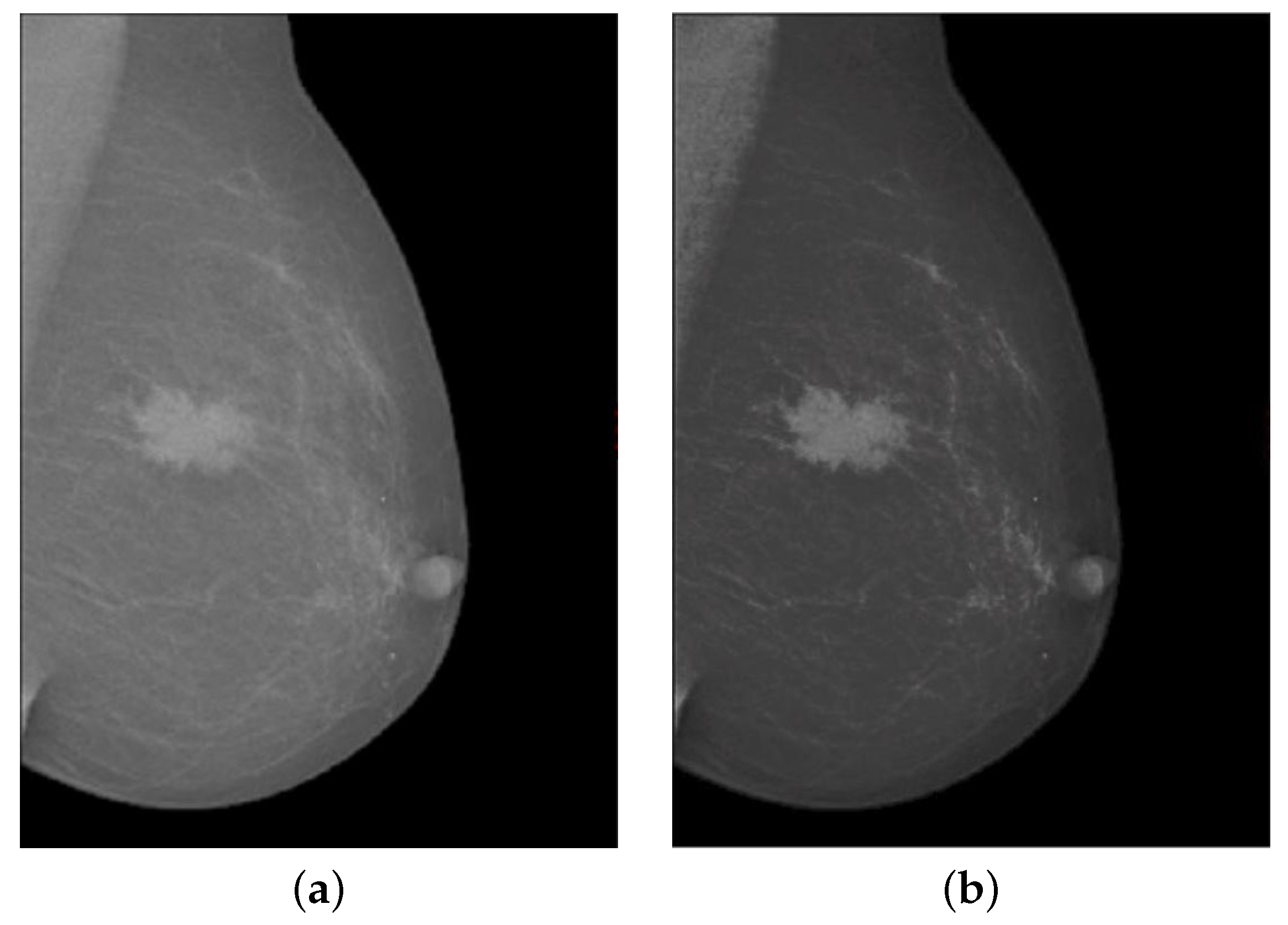
Figure 3 shows the contrast enhancement of the input image. In Figure 3a, the source mammogram image having a tumor is not visible as the tumor in the breast image has no sharp edges. Whereas in Figure 3b image shows that after using the modified contrast enhancement approach, the image gradient has been significantly improved and the disease part is prominently highlighted in the breast mammogram image. Upon closing of this phase, the proposed approach moves to the third phase, which is detailed in the next subsection.

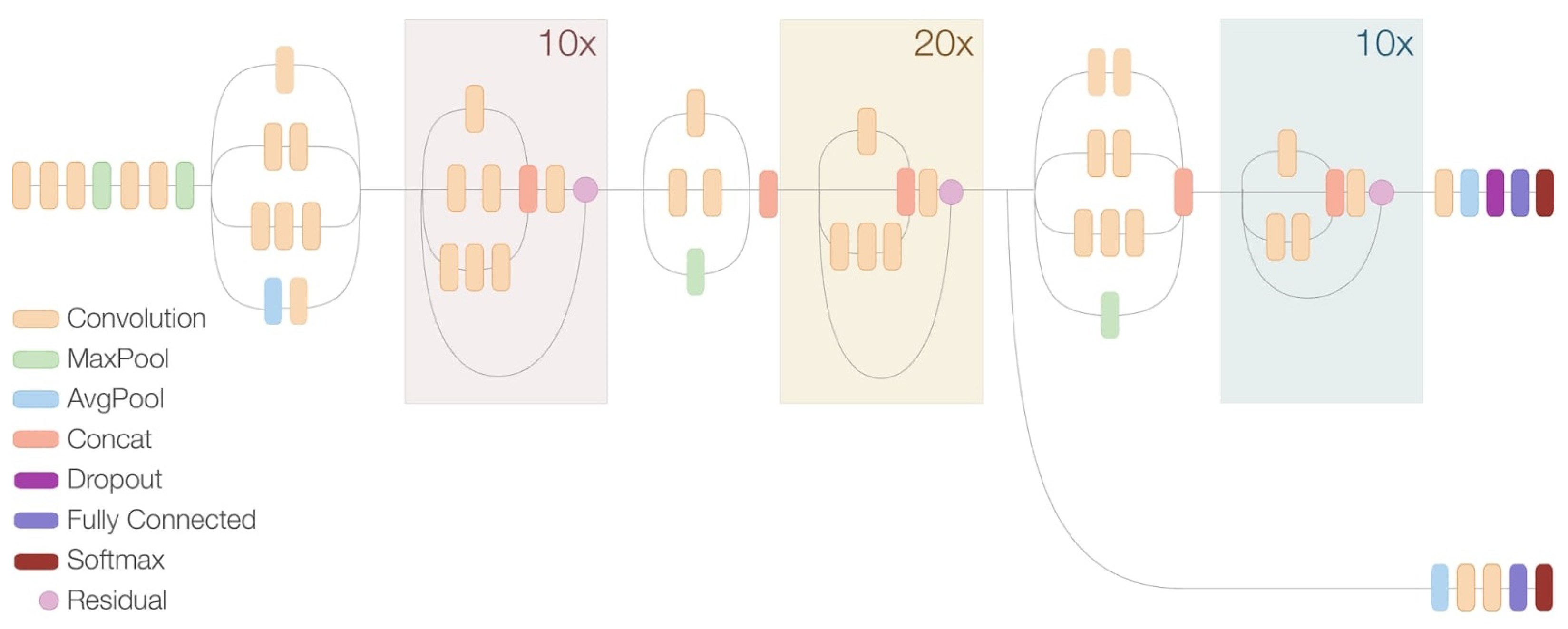
3.3. Network Architecture

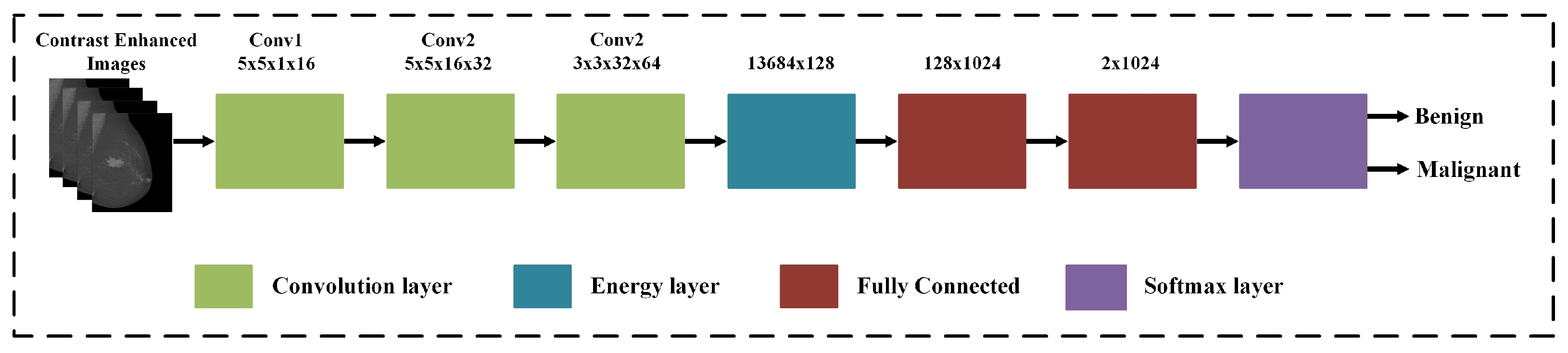
The TTCNN architecture is presented for breast cancer classification. The proposed deep CNN considers the three important features of the image: Firstly, the size of some description patterns is much smaller than the source image, but if their size is equal to the convolution filter mask size, the convolution filter can find the pattern. Secondly, certain shapes or patterns can be used in different parts of the mammogram image. These models can also be defined by convolving the entire source mammogram image. Thirdly, downsampled pixels are very important for the max-pooling layer and do not change the shape of the source mammogram image. The proposed TTCNN framework for the breast cancer classification is illustrated in Figure 4.

The proposed TTCNN contains two convolution layers, followed by the pooling layers and the third convolution layer directs the EL. Then, a softmax layer is used with the fully connected (FC) layer. EL summarizes the feature maps of the last convolutional layer by averaging the rectified activation output. This returns a value for each feature map, equivalent to the energy response to a filter bank. In addition to reducing the number of layers, this architecture offers excellent performance in learning texture functions and requires less computation time and memory. EL enables this trade-off between performance and computation time. This layer is implemented to conserve the data flow of the original layer. The flattened output of EL is redirected to the concatenation layer immediately after the last pooling layer. This connection creates a new flattened vector that contains information about the shape and texture of the image and spreads it to the fully connected layer. The complete description of the proposed network with both the input and output dimensions is given in

Table 2. Proposed texture CNN architecture layers.

Layers	Types	Input Size	Kernel Size to Form Each Feature Map	Stride	Padding	Output Size
1	Convolutional Layer 1	64 × 64 × 1	5 × 5	[1 1]	[1 1 1 1]	62 × 62 × 16
2	Max Pooling Layer 1	62 × 62 × 16	2 × 2	[2 2]	[1 1 1 1]	32 × 32 × 16
3	Convolutional Layer 2	32 × 32 × 16	5 × 5	[1 1]	[1 1 1 1]	30 × 30 × 32
4	ReLU
5	Max Pooling Layer 2	30 × 30 × 32	2 × 2	[2 2]	[1 1 1 1]	16 × 16 × 32
6	Convolutional Layer 3	16 × 16 × 32	3 × 3	[1 1]	[1 1 1 1]	16 × 16 × 64
7	ReLU
8	EL	16 × 16 × 64	-	-	-	128 × 1
9	Dropout	128 × 1	-	-	-	128 × 1
10	FC1	128 × 1	-	-	-	1024 × 1
11	Dropout	1024 × 1	-	-	-	1024 × 1
12	FC2	1024 × 1	-	-	-	2 × 1
13	Softmax Layer		-	-	-
14	Classification Layer		-	-	-

. The output size of the convolution layer is mathematically computed in Equation (8) as:

$$Output=\frac{I_a-I_b+2S}{\varrho +1},$$

(8)

where $I_a$ and $I_b$ represents the input and filter size respectively, S denotes the padding, and $\varrho$ is the stride value.

Afterwards, the three convolution layers are utilized with kernel size of 5 × 5 for the first two layers and the output of these channels are 16 and 32, respectively. The third convolution layer is examined as an intermediate layer for extracting texture properties with kernel size of 3 × 3 having the output channels 64. Only 31,744 parameters can be learned from the convolution layer and these parameters are calculated using the following formulas in Equations (9) and (10) as:

$${\xi }_v={\zeta }_V\times (I_k\times \varrho +1),$$

(9)

$${\xi }_v={\zeta }_V+X_k\times \varrho \times {\zeta }_V,$$

(10)

where ${\xi }_v$ denotes the CNN layer learnable parameters, $I_k$ represents the kernel size, and ${\zeta }_V$ denotes the channel number.

Each convolution layer computes the output of the neuron connected to the input. The calculation is the dot product between its weight and the smallest input field attached to it. The first convolution layer constructs a 16-kernel 32 × 32 × 16 size output. Equation (11) gives the output of the neurons in the first convolution layer as:

$$S_{\vartheta }=\sum _{\vartheta }{C}_{\vartheta }\times T_{\vartheta }+P_{\vartheta },$$

(11)

where $S_{\vartheta }$ represents the output feature maps, $C_{\vartheta }$ represents the input feature maps, and T denotes the weighted map. Afterwards, an energy descriptor is utilized for the output of the final convolution layer. Energy layers are combined after the third convolution layer, taking into account the requirements of the energy descriptor. Its functionality is similar to a dense, messy texture descriptor. The connection is given in Equation (12) as:

$$EL(\xi ,\vartheta )=\rho \left[\sum _{i=1}^j{T}_i^{\omega }{\vartheta }_i+P\right],$$

(12)

where $EL(\xi ,\vartheta$) represents the EL output layer, j represents the input connections, and T represents the EL weighted vector. Compared to the last conventional convolution layer interconnection, the interconnection between the EL and FC layers is much smaller and leads to a reduction in learnable parameters. In addition, EL retains energy information from the preceding layer and learns during forward and backward propagation. Furthermore, to reduce the vector size of the next FC layer, EL also improves the overall learning ability of the network and diminish the complication of the proposed system. Use Equation (13) to calculate the learnable parameters of EL as:

$${\xi }_{EL}={\eta }^m\times {\eta }^{m-1},$$

(13)

where ${\xi }_{EL}$ is the EL learnable parameters, ${\eta }^m$ is the current FC layer neuron, and ${\eta }^{m-1}$ is the previous FC layer neuron.

To speed up the training process the batch normalization and activation function is used between the convolution layer and rectified linear unit (ReLU) layer. Batch normalization is used to remove the internal covariate shift [50]. This can be done by normalizing the mean and standard deviation. The bulk normalization calculation uses the following Equations (14) and (15) to calculate mean and variance.

$${\tau }_Q=\frac{1}{n}\sum _i^n{\iota }_i,$$

(14)

$${\upsilon }_Q=\frac{1}{n}\times \sum _i^n{({\iota }_i-{\tau }_Q)}^2,$$

(15)

where ${\tau }_Q$ and ${\upsilon }_Q$ represents the mean and variance respectively, n is the mini batch size of ${\iota }_i$ element of features. In our work the value of n is 64. The batch normalization is calculated in Equation (16) as:

$${\lambda }_i=\frac{{\vartheta }_i-\tau }{\sqrt{{\upsilon }^2+\varphi }}\alpha +A,$$

(16)

where $\alpha$ and A are initial learnable parameter values of each output layer. ReLU is used as an activation function which is computed in Equation (17) and the output of the ReLU layer is calculated in Equation (18) as:

$${\lambda }_{i,j,k}=max0,{\vartheta }_{i,j,k},$$

(17)

$${\lambda }_{ReLU}=ReLU\left(Bnorm\left(Conv(w,x)\right)\right),$$

(18)

where ${\lambda }_{i,j,k}$ denotes the output element features and ${\vartheta }_{i,j,k}$ denotes the feature of the input element. Afterwards, the pooling layer reduces the size of feature maps, weights, and computations which shows overfitting of the control network. The max pooling layer is mathematically computed in Equation (19) as:

$$M_{pool}=max\left(0,\sum _Q{\vartheta }^{k-1}{T}_{\vartheta }\right),$$

(19)

where $M_{pool}$ represents the output feature maps, $\vartheta$ indicates the input feature maps, Q denotes the pooling size, and T represents the max pooling layer for kernel vector. In this work, two max pooling layers are used with each layer kernel size 2 × 2.

The dropout layer is used to remove a subset of random parameters repeatedly through the weighted update process to avoid overfitting training data. Drop editing is used to remove a subset of random parameters repeatedly during the weighted update process to avoid overfitting training data. FC layers have the most parameters across the network and are therefore subject to over-compatibility of training data. Hence, the dropout layer is determined after the FC layer. The softmax layer is utilized as a classifier which uses the loss function. The range of probability values for softmax is [0, 1]. The mathematical expression of loss function is given in Equation (20) as:

$${\kappa }_l={\delta }_j+log\sum _{i}exp\left({\delta }_i\right),$$

(20)

where ${\kappa }_l$ denotes the total loss and ${\delta }_i$ having the class $\delta$ which is i-th vector element. The purpose of the classifier is to reduce the probability difference between the real label and the estimated label which is calculated using the softmax function in Equation (21) as:

$${\lambda }_i=\frac{ex{p}^{{\delta }_j}}{{\sum }_{i}exp\left({\delta }_i\right)}.$$

(21)

Upon completion of this stage, TTCNN proceeds to the fourth phase, which is explained in the following subsection.

3.4. Deep Feature Extraction Using Transfer Learning

Transfer learning is a deep learning (and machine learning) method that transfers expertise from one model to another. Transfer learning allows us to solve all or part of a specific task by using an already pre-trained model to complete another task. Machines use what they have learned from previous tasks to improve predictions for new tasks in transfer learning. Transfer learning has many benefits, but the most significant is that it reduces training time, enhances the performance of neural networks, and does not make large amounts of data available. Below is a concise description of the state-of-the-art CNN deep feature extraction model which is selected in our work.

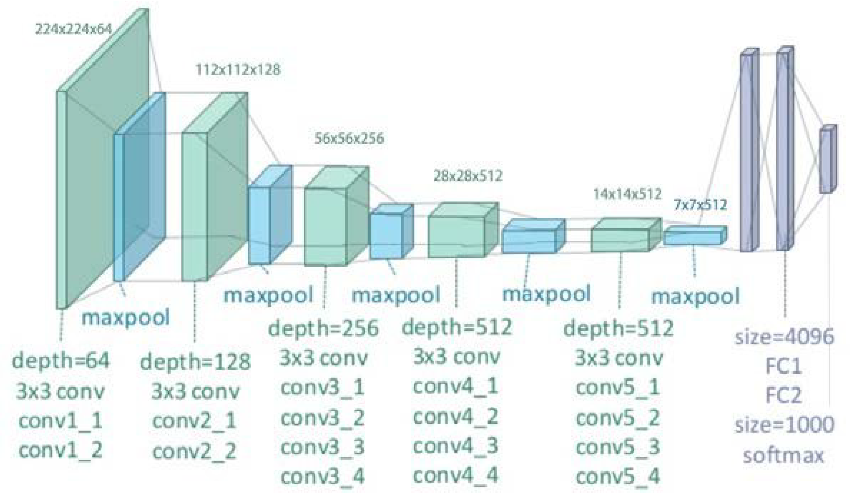
3.4.1. VGGNet

VGGNet is a CNN architecture presented by Andrew Zisserman and Karen Simonyan from the Oxford University in 2014 [41]. It is formulated by intensifying the depth of the accessible CNN architecture to 16 or 19 called VGG-16 and VGG-19, respectively as illustrated in Figure 5.

The VGG-16 architecture contains 138 million parameters and the VGG-19 contains 144 million parameters. The VGG-16 model has 13 convolutional layers, five max pooling layers, and three fully connected layers. VGG has a small filter (3 × 3) instead of a larger filter. It has the same effectual receptive field as having only one 7 × 7 convolutional layer. The VGG-19 model has 16 convolutional layers, five max pooling layers, and three fully connected layers. In the two variants of VGGNet, there are two fully connected layers, each with 4096 channels, and then another fully connected layer with 1000 channels to anticipate 1000 labels.

3.4.2. ResNet

ResNet was founded in 2015 by Kaiming He and the idea behind that is each layer of the framework is determined from the residuary function by referring to its own input layer. This network won the ILSVRC 2015 competition with a lower error rate of 3.57%. In this degree, the ResNet model is certainly optimized and the precision can be greatly improved [40]. For this task, we have used three pre-trained ResNet-18, ResNet-50 and ResNet-101 networks.

Table 3. The RestNet-18, RestNet-50 and RestNet-101 architectures.

Layer Name	Size of Output	ResNet-18	ResNet-50	ResNet-101
Conv1	112 × 112	$7\times 7$, 64 Stride 2 3 × 3 maxpool, Stride 2	$7\times 7$, 64 Stride 2 $3\times 3$ maxpool, Stride 2	$7\times 7$, 64 Stride 2 $3\times 3$ maxpool, Stride 2
Conv2_x	56 × 56	$\left[\begin{array}{c}3\times 3,64\\ 3\times 3,64\end{array}\right]$× 2	$\left[\begin{array}{c}1\times 1,64\\ 3\times 3,64\\ 1\times 1,256\end{array}\right]$× 3	$\left[\begin{array}{c}1\times 1,64\\ 3\times 3,64\\ 1\times 1,256\end{array}\right]$× 3
Conv3_x	28 × 28	$\left[\begin{array}{c}3\times 3,128\\ 3\times 3,128\end{array}\right]$× 2	$\left[\begin{array}{c}1\times 1,128\\ 3\times 3,128\\ 1\times 1,512\end{array}\right]$× 4	$\left[\begin{array}{c}1\times 1,128\\ 3\times 3,128\\ 1\times 1,512\end{array}\right]$× 4
Conv4_x	14 × 14	$\left[\begin{array}{c}3\times 3,256\\ 3\times 3,256\end{array}\right]$× 2	$\left[\begin{array}{c}1\times 1,256\\ 3\times 3,256\\ 1\times 1,1024\end{array}\right]$× 6	$\left[\begin{array}{c}1\times 1,256\\ 3\times 3,256\\ 1\times 1,1024\end{array}\right]$× 23
Conv5_x	7 × 7	$\left[\begin{array}{c}3\times 3,512\\ 3\times 3,512\end{array}\right]$× 2	$\left[\begin{array}{c}1\times 1,512\\ 3\times 3,512\\ 1\times 1,2048\end{array}\right]$× 3	$\left[\begin{array}{c}1\times 1,512\\ 3\times 3,512\\ 1\times 1,2048\end{array}\right]$× 3
Pooling	1 × 1 × 512		Average pooling
FC	512 × 10		Fully connected
Softmax	1000		Softmax

illustrated the basic architecture of all these networks.

The input size of the network is 224 × 224. In the three architectures described, the first convolutional layer and the final three layers, i.e., pooling, FC and the softmax are affixed. If the internal convolution layers number is increased, the depth of the deep network changes.

3.4.3. GoogLeNet

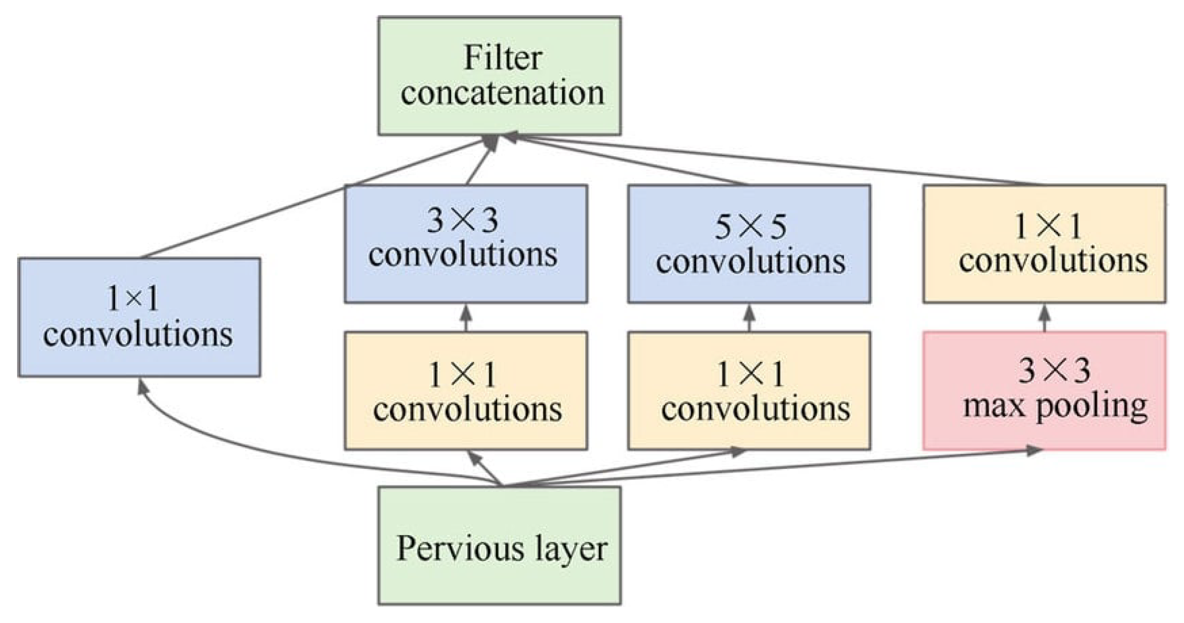
GoogLeNet [43] is a CNN based on the Inception architecture. GoogLeNet (Inception V1) won the ILSVRC 2014 challenge. It reached an error rate of 6.67% which is very near to the human-level performance that challenge organizers must currently assess. The architecture of the Inception block is displayed in Figure 6. It uses the Inception module, which allows the network to choose between several convolution filter sizes for each block. The Inception network occasionally stacks these modules together and uses the maximum max-pooling layer with stride 2 to bisect the resolution of the grid.

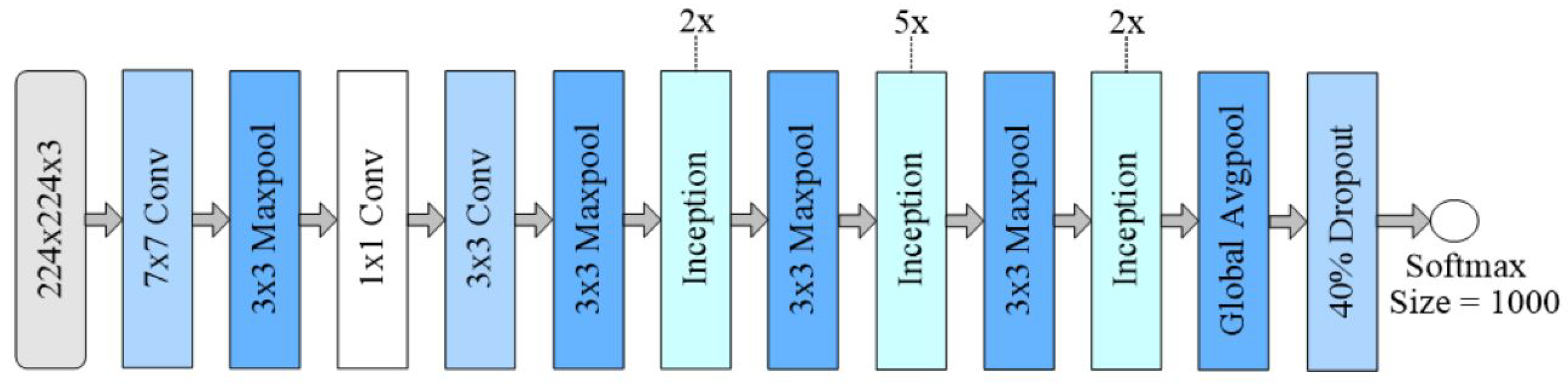
The architecture of GoogLeNet consists of 22 deep CNN layers, but the parameters number is diminished to 4 million from 60 million (AlexNet). It consists of four simultaneous boughs. Convolution layers with kernel sizes of 1 × 1, 3 × 3, and 5 × 5 are used in the first three boughs. The intricacy of the frame can be diminished by convolving two intermediate branches in the input channel with a window size of 1 × 1. Appropriate padding is employed for all four boughs so that the height and width of the inputs and outputs are the same. The final inception block is created after linking the output of each bough. It contains almost 6.8 million parameters. GoogLeNet architecture has nine inception blocks containing 6 convolutional layers, 3 convolutional layers of 1 × 1 (for dimensionality reduction), 3 × 3, and 7 × 7, 4 layers of max-pooling, two layers of normalization layers, average pooling, and FC layer. The ReLU activation function is utilized by all the convolution layers and drop regularization is applied to the FC layer. The softmax function is used in the output layer. The block of GoogleNet is shown in Figure 7.

3.4.4. Inception-ResNet-v2

This network is a form of Inception-v3 [43] which combines a certain design from the ResNet [40]. Inception-ResNet-v2 only uses batch normalization at the traditional layers. To increase the depth of the networks and the number of inception blocks the residual modules are used. The Inception-ResNet-v2 architecture contains one stem block (six convolutional blocks and one max pooling layer) and three different sets of inception blocks. The first block has five inception modules, each with seven convolution blocks. The first block has 10 inception modules, each with five convolution blocks, and the third and last block has five inception modules, each with four blocks of convolution, also contain two depletion blocks with different convolutional layers, average pooling, and FC layers. At the output layer softmax activation function is utilized. Figure 8 illustrates the model of Inception-ResNet-v2.

3.4.5. Inception-v3

This network is also the CNN architecture of the Inception series, including label smoothing, 7 × 7 factoring convolution, and the use of auxiliary classifiers to further propagate label information over the network (batch use), and have been made some improvements, standardization for the sidehead layer. Inception-v3 used 1 million training images from thousands classes of ImageNet datasets for training. Inception v3 showed more than 78.1% accuracy rate on the ImageNet dataset. Over the years, this architecture is the climax of many ideas established by various researchers. The architecture comprises symmetric and asymmetric building blocks, such as convolutional layer, average pooling, max pooling layers, concatenation layer, dropout layer, and FC layer. Batchnorm is widely used throughout the architecture and is suitable for activation input. The loss is calculated using Softmax. This model truncates the number of parameters that can be learned and also truncates the complication of the network. The general framework of the Inception-v3 model is illustrated in Figure 9.

Upon completion of this stage, TTCNN moves to the fifth stage, which is elaborated in the following subsection.

3.5. Feature Fusion

This is the most highlighted field in the pattern recognition [60]. Feature fusion combines the features from different layers or branches. Feature fusion performed from different operations i.e., concatenation and summation. In this regard, the convolutional sparse image decomposition (CSID) fusion approach [28] is employed to interconnect the selected feature vectors in the matrix to obtain feature vectors. The feature fusion is evaluated in Equation (22) as:

$${\chi }_{o,p}=mi{n}_{{\xi }_{o,p}}\frac{1}{2}\parallel O_{\iota }-\sum _{p=1}^{Q_t}{h}_{t,p}\ast {\xi }_{t,p}-\sum _{m=1}^{M_o}{l}_{o,p}\ast {\xi }_{o,p}{\parallel }_2^2+{\diamond }_o\sum _{p=1}^{Q_t}\left|\right|{\xi }_{t,o}{\left|\right|}_1.$$

(22)

This operation continues till all pairs are compared. ${\chi }_{o,p}$ is the final fused vector. Upon termination of this stage, TTCNN approach move to the sixth and last phase, which is discussed in the next subsection.

3.6. Feature Selection

In the last few years, feature selection methods have successfully enhanced the system efficiency and exhibit a prominent improvement in medical imaging [61]. Feature selection is employed to enhance the classification accuracy, annihilate the redundancy among the features, and use only robust features for perfect classification. This allows us to truncate prediction numbers and complete the testing process rapidly. In this regard, an entropy controlled firefly approach (ECfA) for optimal feature selection is used. First, the firefly approach selects the function, then proposes an entropy based activation function, and passes the function to the final selection stage. Yang et al. [62] proposed a firefly approach which is a modern and extensive metaheuristic optimization method caused by the glowing behavior of fireflies. Compared to the particle swarm optimization (PSO) and genetic approach (GA) [63], the firefly approach uses the flicker behavior of fireflies to optimize multimodal problems for robust performance.

The glow of a firefly with original brightness $\gamma$ is expressed in Equation (23) as:

$$\gamma \left(u\right)={\gamma }_{\diamond }{e}^{-\varrho u},$$

(23)

where ${\gamma }_{\diamond }$ represents the original brightness, u represents the distance between two fireflies, and $\varrho$ represents the optical coefficient that causes the brightness and the number of individuals. As we all know, brightness is directly proportional to attractiveness. Therefore, the attractive force $\beta$ is expressed in Equation (24) as:

$$\beta \left(u\right)={\beta }_{\diamond }{e}^{-\varrho u},$$

(24)

when u = 0, the attraction is ${\beta }_{\diamond }$. The firefly attraction s and t is shown in Equation (25) as:

$$H_s^{i+1}={\beta }_{\diamond }{e}^{-\varrho u_{st}^2}(H_t^i-H_s^i)+\eta (Rand-\frac{1}{2}),$$

(25)

where $\eta$ denotes the randomness of the parameters, i is the number of iterations, and $Rand$ initiates random numbers from 0 to 1. The distance between $sth$ and $tth$ fireflies is represented by ${\varsigma }_{st}$ and is calculated in Equation (26) as:

$${\varsigma }_{st}=\parallel H_t-H_s\parallel =\sqrt{\sum _{j=1}^J{(H_{sj}-H_{tj})}^2}.$$

(26)

The minimum distance characteristic is evaluated. The next iteration is executed based on the error rate. We have chosen a total number of iterations n = 100 in our work. After each iteration, the feature vectors ${\phi }_N^{j1}$ and ${\phi }_N^{j2}$ are obtained for the optimal vectors of N × 1746 and N × 1822 dimensions, respectively. The activation function based on entropy is employed for all the features. At this phase, we use an entropy based activation function to further enhance the function. The activation function is determined as:

$$B\left(\phi \right)=-\sum _{i=1}^{j}H\left({\phi }^j\right)lo{g}_{2}H\left({\phi }^j\right),$$

(27)

$$\widehat{{\phi }_N^{j1}}=\{\forall {\phi }_N^{j1}\ge B\left(\phi \right)\},$$

(28)

$$\widehat{{\phi }_N^{j2}}=\{\forall {\phi }_N^{j2}\ge B\left(\phi \right)\},$$

(29)

where j∈($j1$,$j2$), $\widehat{{\phi }_N^{j1}}$ and $\widehat{{\phi }_N^{j2}}$ is an optimal feature for ${\phi }_N^{j1}$ and ${\phi }_N^{j2}$ respectively. In our work, the optimal length of the feature vector after applying the activation function is N × 1346 and N × 1322 respectively.

The ECfA based feature selection approach is also detailed in Algorithm 1.

Algorithm 1 Feature Optimization based on Entropy Controlled Firefly

Input: Results from CSID fusion approach. Output: Optimal features selection. Step 1. Fitness function $p\left(x\right)$, x = ($x_1$,$x_2$,$x_3$,…,$x_m$) Step 2. Generate initial firefly populations $H_s$, where $s=1,2,3,\dots ,n$ Step 3. Calculate brightness ${\gamma }_{\diamond }{e}^{-\varrho u}$ Step 4. Absorption coefficient $\varrho$     while (r ≤ Maximum Generation) do         for s = 1:t do                for t = 1:s do                        if (${\gamma }_s$ > ${\gamma }_t$) then                                    ∘ Attraction depends on distance $\varsigma$, $e^{\varrho u}$                                    ∘ Move the firefly s in the direction of t using $H_s^{i+1}={\beta }_{\diamond }{e}^{-\varrho u_{st}^2}(H_t^i-H_s^i)+\eta (Rand-\frac{1}{2})$                                    ∘ Estimate new solutions and upgrade brightness                        end if                end for s         end for t         Step 5. Find the best fireflies         Step 6. The activation function based on entropy is employed B($\phi )$         Step 7. Best optimal feature vector are selected $\widehat{{\phi }_N^j}$     end while     Step 8. Processing and visualization of results end

4. Performance Evaluation

This section examines the experiment and validation of the proposed TTCNN approach for mammogram imaging. Descriptions of benchmark datasets, evaluation metrics and comparison with other state-of-the-art approaches have also been discussed.

4.1. Simulation Setup

The experiments are implemented in MATLAB R2021a (MathWorks Inc., Natick, MA, USA) on a laptop for simulation results. The hardware platform comprises the Intel(R) Core(TM) i7 9750H CPU 2.59 GHz processor (Intel Corporation, San Francisco, CA, USA) with 12 GB RAM and GPU of NVIDIA GeForce GTX 1650 (NVidia Corporation, Santa Clara, CA, USA) in Microsoft Windows 11 (Microsoft, WA, USA).

4.2. Image Acquisition

In this study, the digitized mammogram images from DDSM [56], INbreast [57] and MIAS [58] datasets are used to evaluate the performance of the proposed method. In fact, all the databases are utilized to show the reliability and effectiveness of the proposed method in diagnosing breast cancer. The DDSM database consists of 1500 mammogram images having 519 normal images and 981 abnormal images. The INbreast database contains 336 mammogram images having 69 normal images and 269 abnormal images, whereas the MIAS database consists of 326 total mammogram images having 207 normal images and 119 abnormal images. In this work, a total of 1369 breast mammogram images were utilized for abnormal, in which the DDSM dataset have 479 benign and 502 malignant out of 981 mammogram images, the INbreast dataset contain 269 mammogram images having 220 benign and 49 malignant, and the MIAS dataset contain 119 mammogram images having 68 benign and 51 malignant [56]. To evaluate the supremacy and effectiveness of the proposed method. Experts collect ground truth labels and diagnose these cases (via labels) using a variety of tests including experimental screening and mammography.

Table 4. Database specifications (normal and abnormal).

Database	Total Number of Images		Training		Testing
	Normal	Abnormal	Normal	Abnormal	Normal	Abnormal
DDSM	519	981	311	589	208	392
INbreast	67	269	40	162	27	107
MIAS	207	119	125	71	82	48

and

Table 5. Database specifications (benign and malignant).

Database	Total Number of Images		Training		Testing
	Benign	Malignant	Benign	Malignant	Benign	Malignant
DDSM	479	502	287	302	192	200
INbreast	220	49	132	29	88	20
MIAS	68	51	40	31	28	20

illustrated the mammography images distribution from the used databases. During the assessment, the images in each database are divided into two sets, a training set and a testing set.

4.3. Performance Evaluation Criteria

The cross-validation approach is developed to enhance the efficiency, validity of performance and to verify the outcome of each database. To analyze the classification efficiency of our proposed approach several metrics are used i.e., accuracy ($Acc$), sensitivity ($Sen$), specificity ($Spe$), error rate ($Er$), matthews correlation coefficient ($Mcc$), Jaccard ($Jac$), positive predicted value ($PPV$), F1 score ($F1$), and area under receiver operating characteristic (ROC) curve also called the area under curve (AUC). These parameters are utilized as measurable elements to compare the proposed method performance with state-of-the-art algorithms. These measured values are defined as follows:

$$Accuracy\left(Acc\right)=\frac{(TP+TN)}{(TP+FP+TN+FN)}\times 100\%,$$

(30)

$$Sensitivity\left(Sen\right)=\frac{TP}{(TP+FN)}\times 100\%,$$

(31)

$$Specificity\left(Spe\right)=\frac{TN}{(TN+FP)}\times 100\%,$$

(32)

$$ErrorRate\left(Er\right)=\frac{FP+FN}{(TN+FP+FN+TN)}\times 100\%,$$

(33)

$$Mcc=\frac{TP\ast TN-FP\ast FN}{\sqrt{(TP+FP)(TP+FN)(TN+FP)(TN+FN)}}\times 100\%,$$

(34)

$$Jaccard\left(Jac\right)=\frac{TP}{(TP+FP+FN)}\times 100\%,$$

(35)

$$PPV=\frac{TP}{(TP+FP)}\times 100\%,$$

(36)

$$F1score\left(F1\right)=2\times \frac{Precision\times Recall}{Precision+Recall},$$

(37)

where $TP$ represents true positive values which correctly recognized the disease cases, $TN$ stand for true negative values which correctly identified the healthy cases, $FP$ stand for false positive values which incorrectly identified the disease cases, and $FN$ stand for false negative values which incorrectly identified the healthy cases.

4.4. Breast Cancer Classification Using Extracted Deep Features with TTCNN

The proposed TTCNN classification approach extracts deep CNN features. The results are acquired by the feature extraction from the optimal layers of every deep CNN model. We selected the best features for all deep CNN frameworks by determining the best feature extraction layer that can deliver the finest performance on TTCNN. To do this, we extract features from different layers, assess the performance of each deep CNN and identify the best layer.

Table 6. Best performance from optimal layers.

Model	Layer	Optimal Layer
InceptionResNet-V2	813	‘activation_203’
Inception-V3	313	‘predictions’
VGG-16	33	‘fc6’
VGG-19	39	‘fc6’
GoogLeNet	140	‘pool5-7x7_s1’
ResNet-18	64	‘res5b_branch2b’
ResNet-50	169	‘activation_48_relu’
ResNet-101	342	‘res5c’

illustrates the best performance results for deep feature extraction from the optimal layers.

The TTCNN classifier from optimal layers features are also analyzed using the evaluation metrics.

Table 7. Best performance from optimal layers. Best values are emphasized in bold.

Model	Sensitivity (%)	PPV (%)	Accuracy (%)	Error rate (%)
InceptionResNet-V2	82.69	85.53	81.74	18.26
Inception-V3	85.43	87.69	84.03	15.97
VGG-16	76.98	77.09	81.41	18.59
VGG-19	77.83	81.51	84.38	15.62
GoogLeNet	82.37	90.04	88.54	11.46
ResNet-18	87.25	83.02	87.68	12.32
ResNet-50	83.38	87.31	82.87	18.58
ResNet-101	89.51	87.64	88.12	11.88

illustrates the classification result with features from the optimal layers.

From the above Table 7, it can be perceived that the GoogLeNet provides the best performance than the other deep CNN models with an accuracy rate of 88.54% and an error rate of 11.46%. Although ResNet-101 is also very close to GoogLeNet with an accuracy rate of 88.12% and an error rate of 11.88%. ResNet-18 also provides very decent performance with an accuracy rate of 87.68% and an error rate of 12.32%. Among all the models, VGG-16 comes last with an accuracy rate of 81.41% and an error rate of 18.59%.

4.5. Classification Results

The proposed TTCNN method classifies mammogram images of breast tumors as benign or malignant. The experiments are performed on DDSM, INbreast, and MIAS databases. The classification accuracy of the proposed TTCNN approach using three different databases is illustrated in

Table 8. Summary of breast cancer detection.

Database	Total Number of Images		Correctly Detected		Accuracy (%)
	Benign	Malignant	Benign	Malignant
DDSM	479	502	474	498	99.08
INbreast	220	49	215	47	96.82
MIAS	68	51	66	49	96.57

. The total training samples of 287 benign and 302 malignant are selected and the total testing samples of 192 benign and 200 malignant are selected for the DDSM dataset and obtained an accuracy of 99.08%. Similarly, the total training samples selected for INbreast are 132 benign and 29 malignant while testing samples are 88 benign and 20 malignant and achieved an accuracy of 96.82%. The total training samples of 40 benign and 31 malignant are selected and the total testing samples of 28 benign and 20 malignant are selected for the MIAS dataset and achieved an accuracy of 96.57%.

The quantitative comparison of the proposed TTCNN method is also compared with other existing state-of-the-art algorithms for each database. The proposed approach appears to outperform other state-of-the-art approaches with high values of accuracy, specificity, sensitivity, and F1 score as illustrated in

Table 9. Performance comparison with respect to DDSM database. Best values are emphasized in bold. N.A—the data is not provided.

Authors	Method	Accuracy (%)	Specificity (%)	Sensitivity (%)
Sadad et al. [22]	Ensemble	93.1	88	95
Muduli et al. [45]	MFO-ELM	98.8	97.22	96.2
Mohanty et al. [64]	ANN	98.18	N.A.	N.A.
Xie et al. [65]	ELM	95.73	97.16	94.88
Mohanty et al. [66]	WC-SSA	98.63	97.37	98.77
Zhang et al. [67]	AdaBoost	90.91	97.38	82.96
Our Proposed Method	TTCNN	99.08	98.96	99.19

,

Table 10. Performance comparison with respect to INbreasrt database. Best values are emphasized in bold. N.A.—data not provided.

Authors	Method	Accuracy (%)	Specificity (%)	Sensitivity (%)
Al-antari et al. [4]	CNN	95.32	N.A.	N.A.
Dhungel et al. [7]	AlexNet	91.0	N.A.	N.A.
Al-antari et al. [8]	AlexNet	95.64	N.A.	N.A.
Carneiro et al. [34]	AlexNet	86	N.A.	N.A.
Zhang et al. [67]	AdaBoost	87.93	97.73	57.20
Our Proposed Method	TTCNN	96.82	97.68	95.99

and

Table 11. Performance comparison with respect to MIAS database. Best values are emphasized in bold. N.A.—data not provided.

Authors	Method	Accuracy (%)	Specificity (%)	Sensitivity (%)
Mohanty et al. [64]	SVM	95.5	96.65	95.81
Xie et al. [65]	ELM	96.02	94.32	95.29
Pezeshki et al. [68]	ANN	61	77	95.03
Tatikonda et al. [69]	MLP	93.37	92.43	94.18
Pashoutan et al. [70]	ANN	94	96.67	90
Our Proposed Method	TTCNN	96.57	97.03	96.11

. The best value is highlighted in bold text.

Table 9 illustrates the quantitative comparison of our proposed approach with existing state-of-the-art algorithms for the DDSM database. The proposed method results yielded superior performance for the DDSM dataset and achieved an accuracy of 99.08%, specificity of 98.96%, and sensitivity of 99.19%. Mohanty et al. [66] also exhibit better performance than the remaining methods as it has the accuracy of 98.63%. However, our approach has better accuracy, specificity, and sensitivity when compared with other algorithms as indicated by the bold text. Table 10 illustrates the comparison for the INbreast database where the proposed approach showed enriched performance and attained an accuracy of 96.82%, specificity of 97.68%, and sensitivity of 95.99%. and outperformed other methods quantitatively. The accuracy result obtained by Al-antari et al. [8] is slightly better than the other approaches which is 95.64%. But still the proposed approach exhibits best performance for the INbreast database when compared with other approaches. Table 11 displays the comparison for the MIAS database where the proposed approach still reveals superior performance and surpasses all the existing state-of-the-art approaches and achieved an accuracy of 96.57%, specificity of 97.03%, and sensitivity of 96.11%. The proposed approach improves breast cancer detection and classification performance in comparison. The proposed approach can be utilized for real-time assessment and assist radiologists for automated analysis of mammogram images.

There may be performance differences when performing the same method on different datasets for specific reasons, i.e., background noise of a source image, illumination, occlusion, model overfitting, unrepresentative data samples, or the probability of the method. Inadequate evaluation of the model can lead to poor performing methods being pushed into production or suppressed under the assumption that the model is overfitted.

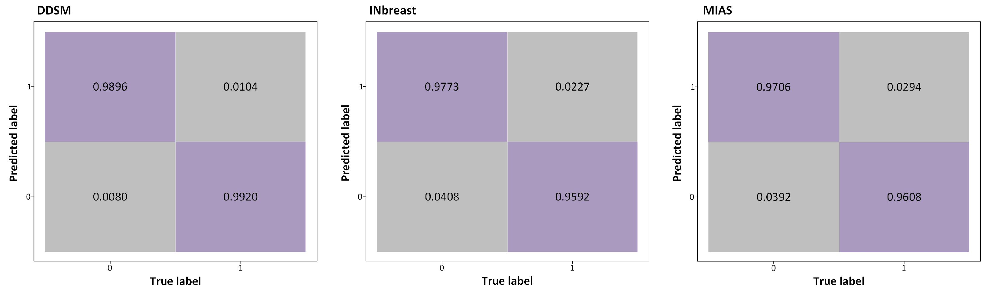
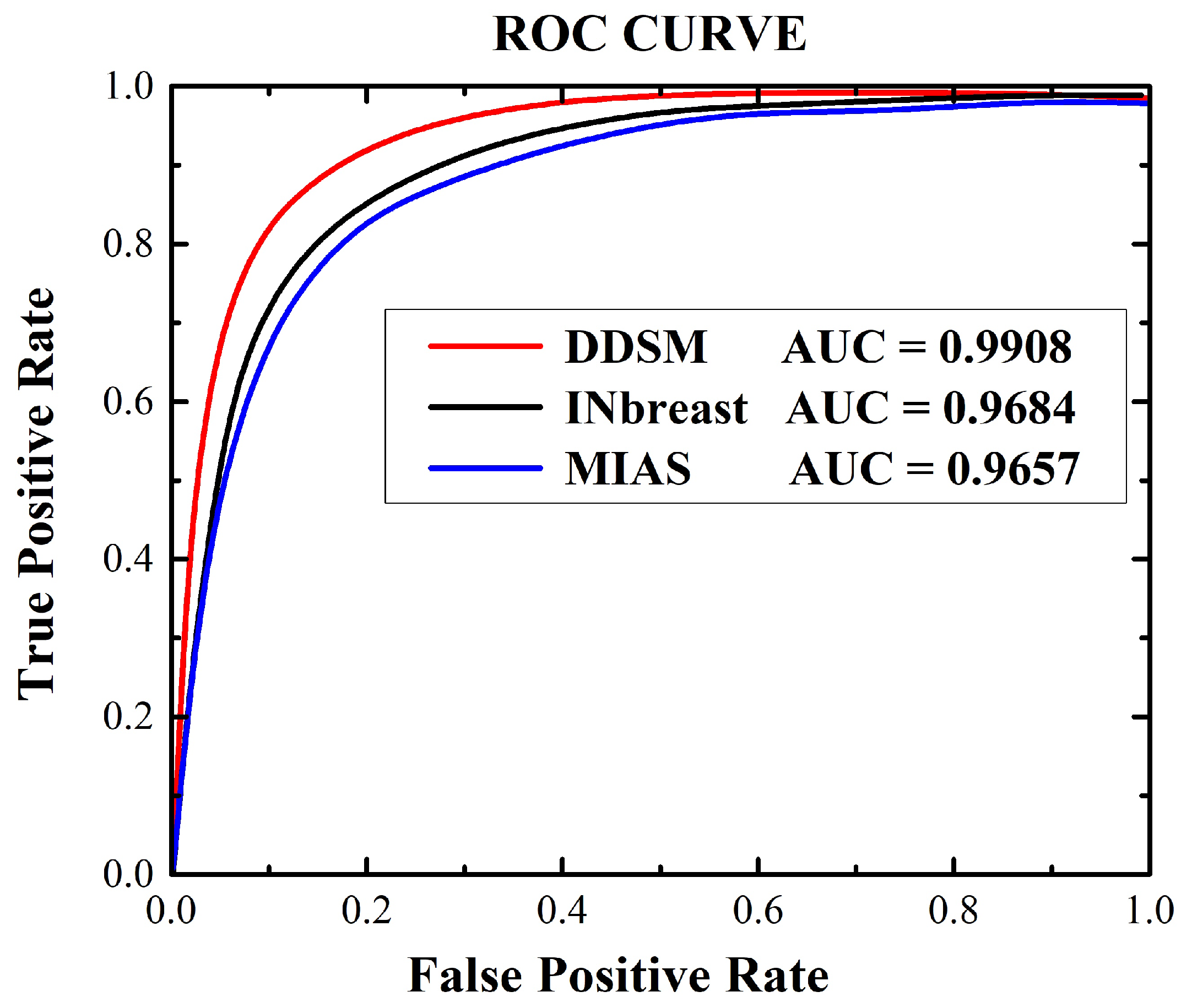
The performance of the proposed approach is also determined utilizing the ROC curves and Confusion Matrix. The confusion matrix of DDSM, INbreast, and MIAS datasets is illustrated in Figure 10. AUC is an important quantitative metric in the ROC curve. The ROC curves were drawn for false positive (1-specificity) and true positive (sensitivity) rates controlling the thresholds of the obtained probability maps. The AUC computations values are estimated for the DDSM, INbreast, and MIAS databsets. The ROC curve graph is illustrated in Figure 11.

The results of breast cancer detection grading (with 95% confidence intervals) are presented in

Table 12. Results of breast cancer detection and classification with 95% confidence interval (CI).

Database	Accuracy (%)	Sensitivity (%)	Specificity (%)	PPV (%)	F1 score (%)	Jaccard (%)	Mcc (%)	AUC (%)
DDSM	99.08 (99.05–99.11)	99.19 (99.16–99.21)	98.96 (98.94–98.99)	98.96 (98.94–98.98)	99.06 (99.03–99.09)	98.19 (98.17–98.21)	98.16 (98.12–98.19)	99.08 (99.07–99.09)
INbreast	96.82 (96.79–96.86)	95.99 (95.96–96.12)	97.68 (97.66–97.70)	97.73 (97.70–97.76)	96.85 (96.83–96.87)	93.89 (93.86–93.92)	93.66 (93.64–93.68)	96.84 (96.80–96.88)
MIAS	96.57 (96.55–96.59)	96.11 (96.10–96.13)	97.03 (97.01–97.05)	97.06 (97.03–97.09)	96.58 (96.53–96.63)	93.39 (93.35–93.43)	93.14 (93.10–93.17)	96.57 (96.54–96.61)

that exhibits the data from aforesaid datasets (DDSM, INbreast, and MIAS). The proposed approach gives the PPV, F1, Jac, Mcc, Er, and AUC of 98.96%, 99.06%, 98.19%, 98.16%, 0.92%, and 99.08% on DDSM, 98.96%, 99.06%, 98.19%, 98.16%, 3.17%, and 99.08% on INbreast, and 97.06%, 96.58%, 93.39%, 93.14%, 3.43%, and 96.57% on MIAS datasets, respectively.

Over the past decade, non-invasive applications such as breast cancer detection and classification have become very prevalent among medical professionals, making the diagnostic process simpler and more accurate [71,72]. TTCNN aims to improve clinical diagnosis by improving breast cancer detection and classification. Based on the accuracy produced by a certain algorithm, we obtained the opinion of two medical experts (one radiologists and one physician). These experts praised the improved results of TTCNN compared to other state-of-the-art approaches.

4.6. Computational Efficiency of Deep Learning Classification

Table 13. Computational time for breast cancer classification.

Database	Time of Training/Epoch (s)	Time of Testing/Image (s)
DDSM	102	1.2
INbreast	31	1.7
MIAS	27	0.4

shows the time execution (in seconds) of the training and testing for each dataset image. In the training set, the number of mammogram images directly alter the time it takes to finish the learning process. Using the TTCNN approach the DDSM dataset takes longer time to train than the INbreast and MIAS datasets. It takes approximately 3.2, 1.4 and 1.1 h to complete the 120 epoch training process on the DDSM, INbreast and MIAS datasets, respectively. For the testing process, the proposed approach took only 1.2 (s) for DDSM, 1.7 (s) for INbreast, and 0.4 (s) for MIAS to classify a single mammogram image. The runtime minimization will be further enhanced in future work, as our main goal is to enhance the detection and classification accuracy.

In general, the proposed approach improves the performance in comparison. The proposed approach can be employed for real-time assessment and assist the radiologists in automated evaluation of mammogram images.

5. Conclusions

In the last few years, diagnostic computer systems based on image processing have been extensively used. This can help radiologists, and minimize the time of diagnosis. Several breast cancer detection and classification algorithms have been presented to enhance medical image analysis. These algorithms have various deficiency, i.e., false diagnosis and prediction; the tumor appears in a area with significantly lower contrast, high complexity of memory, computationally complex approach and require more treatment time to identify the accurate tumor, and current deep learning algorithm need extensive training data to overcome the problems of overfitting and high computational cost.

This article intended to resolve the aforementioned issues by the proposed TTCNN-based classification approach for breast cancer detection and classification. Firstly, the source mammogram images are pre-processed by employing the modification to the legacy CLAHE approach. Then, by using TTCNN architecture, the breast cancer regions that are malignant and benign are classified from the mammogram images and the EL examines the texture features and extracts the general information of shape, limit the size of the output vector, and refines the model’s overall learning ability. Deep features are extracted from eight state-of-the-art DCNN models and optimal layers for feature extraction are determined by monitoring fluctuations in classification performance using a succession of experiments to select the best deep features. Afterwards, the features are fused using the CSID fusion algorithm, and for the robust feature selection an ECfA approach is used.

The proposed approach was applied to DDSM, INbreast, and MIAS datasets, and obtained an accuracy of 99.08%, 96.82%, and 96.57%, respectively. In addition, the proposed approach is visually gratifying, provides better results, and is more capable in the detection and classification of breast mammograms and outperforms other systems. Breast images are accurately detected and classified in less computation time and give pleasant results. In the future, this work will be explored for other application areas of biomedical imaging such as brain tumor detection.