1. Introduction
Thailand is a biodiverse country with a vast array of flora and fauna. Fungi, commonly known as mushrooms, make up a significant portion of these species and play a role in the lifecycles of many living organisms. Moreover, mushrooms are highly nutritious, a good source of protein, low in calories and unsaturated fats, and a rich source of vitamins and iron [
1]. The most popular species are eaten as vegetables in several meals. Mushrooms are also economically important, as wild mushrooms are gathered and sold. Mushrooms can be found after 2–3 days of rain between May and September. Mushrooms appear in large numbers in the dipterocarp forests, mixed forests, and dry evergreen forests in the north and northeastern parts of Thailand. There are between two and three million different species of mushrooms in the world, and these can be divided into two types: poisonous and edible [
2,
3,
4]. Certain poisonous mushrooms have very similar appearances to edible mushrooms. According to folk wisdom, classifying mushrooms as poisonous or edible involves boiling mushrooms in the same pot as rice: a change in the color of the rice demonstrates that the mushrooms are poisonous. A silver spoon changing from silver to black when used to stir a pot of boiling mushrooms is another folk method used to identify poisonous mushrooms. However, the above experiments are not precise, as certain poisonous mushrooms do not respond to these tests. The basic morphological characteristics of poisonous mushrooms are the presence of bright, colorful scales on the cap and a circle under the cap. Inexperienced gatherers can easily make a mistake. Poisonous mushrooms affect the nervous system, leading to death if consumed in high quantities [
5]. Every year, people die from eating poisonous mushrooms in Thailand.
Deep learning, which is part of the machine learning (ML) concept, automates learning by mimicking the operation of the human brain. It involves the implementation of multiple layers of neural networks, allows for complex processing, and is highly accurate. Additionally, deep learning methods are more accurate than human classifiers because they are trained by large datasets. A model can be trained using sample data, and its accuracy depends on the amount of sample data used. Presently, deep learning is used in various fields, such as facial recognition [
6,
7], plant disease detection [
8,
9], and autonomous vehicles, for object classification to increase the speed of work [
10,
11]. Deep learning consists of three components: the input layer, the hidden layer, and the output layer.
The proposed model was used to improve the AlexNet convolutional neural network in order to increase the speed and maintain the accuracy when classifying poisonous and edible mushrooms. The authors hope that this may reduce the number of deaths caused by the consumption of poisonous mushrooms. The results of the proposed model were compared with those of three pretrained architectures, AlexNet, ResNet-50, and GoogLeNet, for the classification of five species of poisonous and edible mushrooms: Inocybe rimosa, Amanita phalloides, Amanita citrina, Russula delica, and Phaeogyroporus portentosus.
2. Related Work
2.1. Convolutional Neural Network (CNN)
A convolutional neural network, a multiple-layer neural network model, is a popular deep learning algorithm that is used for image analysis and object recognition [
12]. The CNN contains convolutional layers, pooling layers, a rectified linear unit, fully connected layers, and a softmax layer [
13,
14,
15]. The structure of the CNN is shown in
Figure 1.
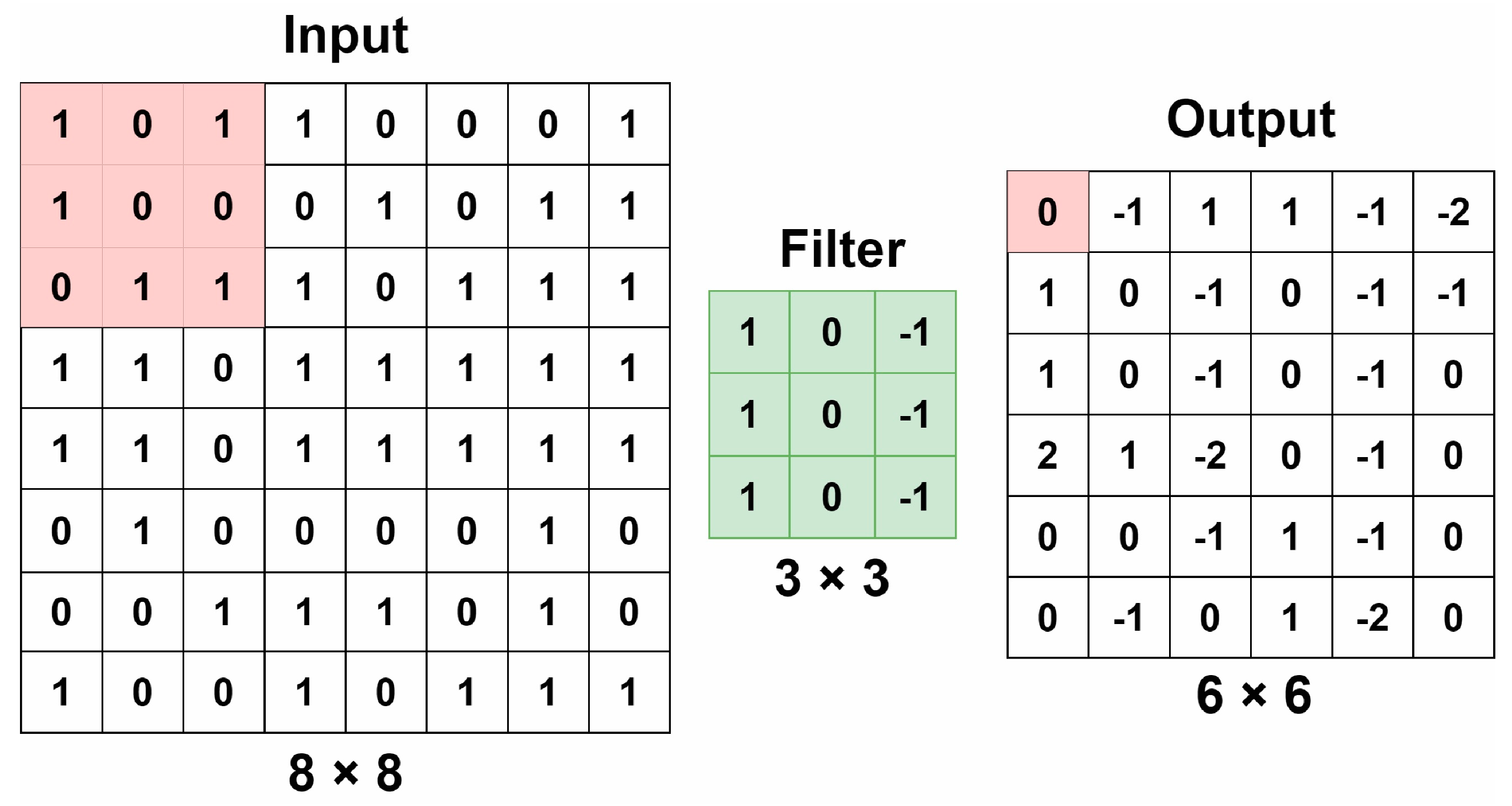
The convolution layer uses filters to extract features from an image [
16]. The filters are smaller than the input because they scroll through each portion of the image to detect features. An example using a 3 × 3 filter is shown in
Figure 2.
The rectified linear unit (ReLU) is a nonlinear activation function. This layer has a value of zero if the input is negative, but it will return the value
x when the input is positive [
17]. ReLU is defined by the following equation:
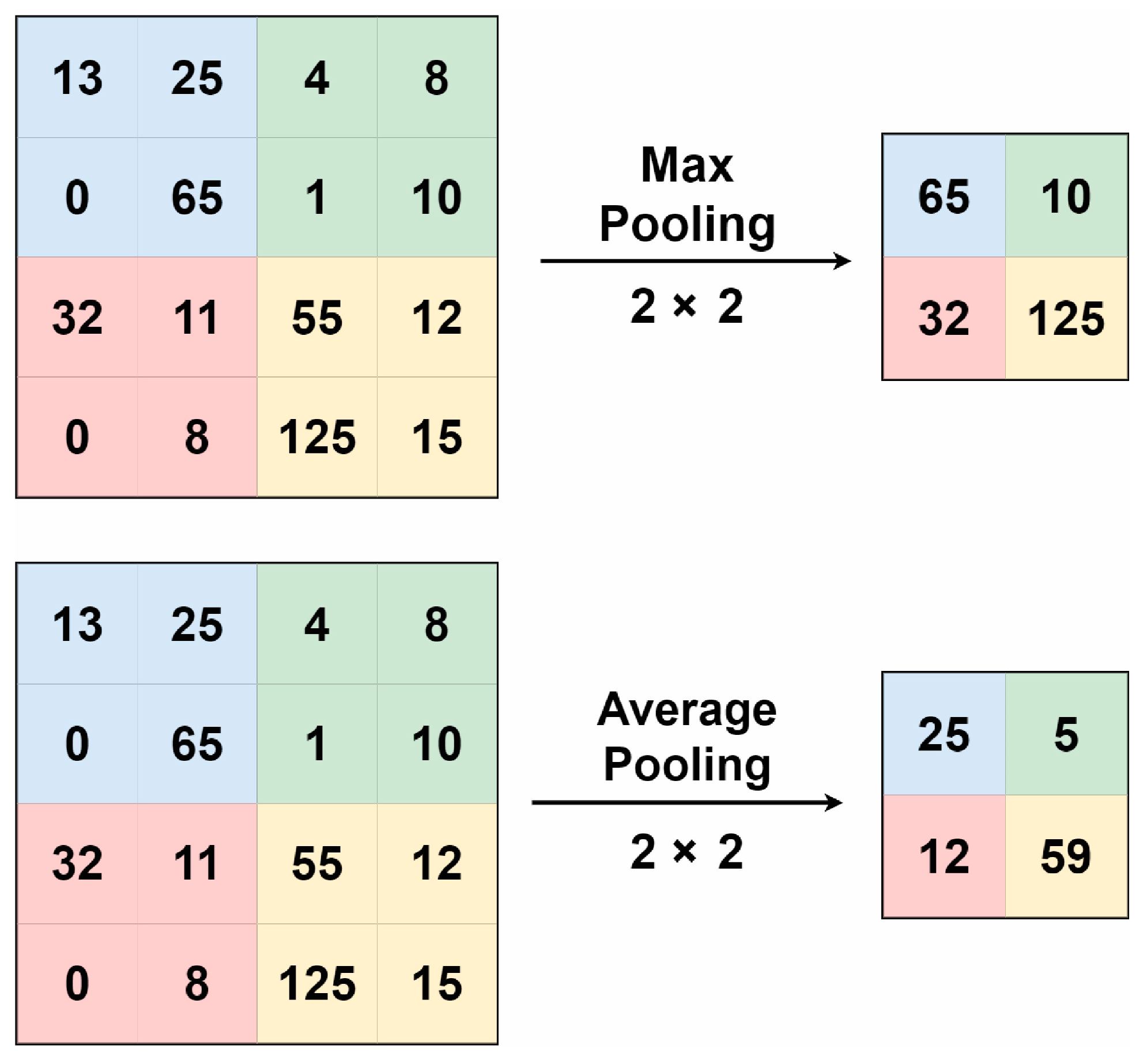
The pooling layer reduces the number of parameters and, depending on the pool size, minimizes the complexity of the output and reduces the training time [
12,
18,
19]. There are different types of pooling: max pooling, average pooling, global average pooling, global max pooling, mixed pooling, L
p pooling, stochastic pooling, spatial pyramid pooling, and region of interest pooling [
20,
21,
22,
23]. An example of max pooling, with a pooling size of 2 × 2, is shown in
Figure 3.
The flattened layer converts the multidimensional data to one dimension before forwarding them to a fully connected layer.
The fully connected layer connects all of the neurons by combining all properties extracted from the previous layer for use in classifying the following layer [
16,
24].
The softmax layer is a functional layer that takes the input and returns the probability of classifying objects [
17].
2.2. Region Convolutional Neural Network (R-CNN)
A CNN is designed to classify objects; however, it does not detect objects or draw bounding boxes around objects. Therefore, the R-CNN method was proposed for object detection and to draw bounding boxes around objects [
25]. In addition to the R-CNN method, there are many other models, such as Fast-RCNN and Faster-RCNN. In this research, the R-CNN method was used because it is a basic method that can detect objects without complexity, and it can easily be modified. The R-CNN consists of four operational steps: first, a selective search of the image is used to extract 2000 region proposals, and each proposal is reshaped to the same size and passed on as an input to a CNN. Second, the CNN uses feature extraction for each region proposal [
26]. Third, upon obtaining the extractions, these features are used to classify region proposals using the SVM. Finally, bounding boxes are created around objects. The R-CNN architecture is shown in
Figure 4.
2.3. AlexNet Architecture
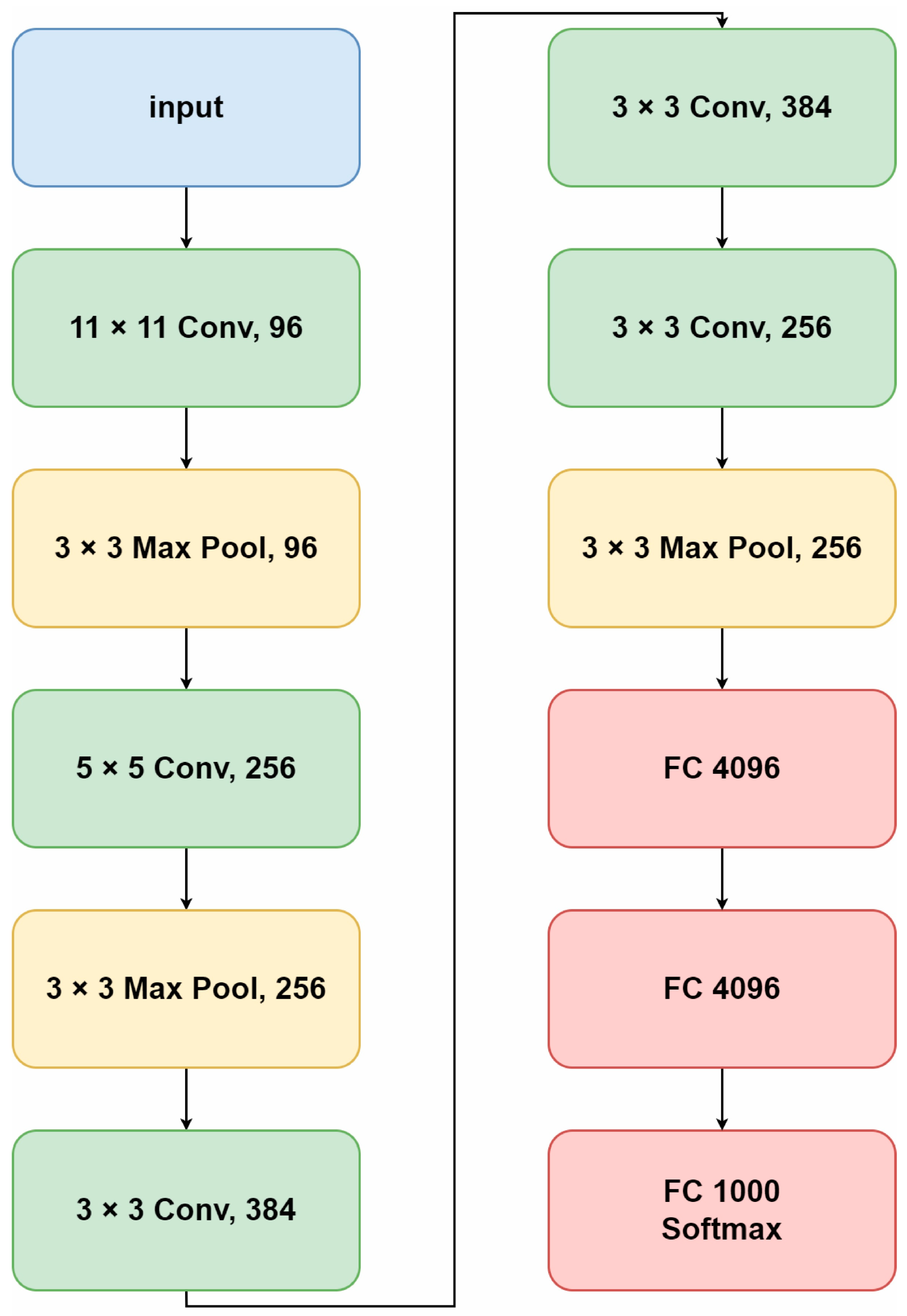
AlexNet is a CNN with eight layers; the architecture has five convolution layers, three max pooling layers, and three fully connected layers [
27,
28]. AlexNet was trained on more than one million images and over 1000 categories from the ImageNet database. It has an image input size of 227 × 227 × 3 pixels: 227 refers to the width and height of the input images and 3 distinguishes the images as RGB color images. The first convolution layer consists of 96 filters with a filter size of 11 × 11 and four strides. The second convolution layer consists of 256 filters with a filter size of 5 × 5 and one stride. The third convolution layer consists of 384 filters with a filter size of 3 × 3 and one stride. The fourth convolution layer consists of 384 filters with a filter size of 3 × 3 and one stride. The fifth convolution layer consists of 256 filters with a filter size of 3 × 3 and one stride. The convolution layer is shown in
Table 1. Afterwards, each convolutional layer is normalized using ReLU and max pooling with a pool size of 3 × 3 [
29,
30]. The AlexNet architecture is shown in
Figure 5.
2.4. ResNet-50 Architecture
ResNet-50 is a CNN that is fifty layers deep. The architecture has an image input size of 224 × 224 × 3 pixels, 16 bottleneck building blocks, 48 convolution layers, and 1 fully connected layer [
31,
32]. It contains both the same and different bottleneck building blocks, as shown in
Figure 6. Bottleneck building blocks numbers 1 to 3 contain convolution layers with 64 filters with a filter size of 1 × 1, another layer with 64 filters with a filter size of 3 × 3, and 256 filters with a filter size of 1 × 1. Building block numbers 4 to 7 contain two convolution layers with 128 filters with filter sizes of 1 × 1 and 3 × 3, respectively, and a convolution layer with 512 filters with a filter size of 1 × 1. Building block numbers 8 to 13 contain two convolution layers with 256 filters with filter sizes of 1 × 1 and 3 × 3, respectively, and another layer with 1024 filters with a filter size of 1 × 1. Building block numbers 14 to 16 contain two convolution layers with 512 filters with filter sizes of 1 × 1 and 3 × 3, respectively, and another layer with 2048 filters with a filter size of 1 × 1 [
33]. There are various ResNet models, e.g., ResNet-18, ResNet-50, and ResNet-101. The ResNet-50 architecture is shown in
Figure 7.
2.5. GoogLeNet Architecture
GoogLeNet is a CNN that is 22 layers deep [
34]. It has an image input size of 224 × 224 × 3 pixels and was designed to incorporate the concept of an inception module [
35]. The inception module contains a convolutional filter with a filter size of 1 × 1, a convolutional filter with a filter size of 3 × 3, a convolutional filter with a filter size of 5 × 5, and a 3 × 3 max pooling pool [
36,
37,
38]. GoogLeNet was designed to have nine inception modules, as shown in
Figure 8. When data are sent to a module, they are divided into four groups and merged into one set when leaving the module. The inception module is shown in
Figure 9.
3. Experimental Section
This section discusses the architecture used for learning and presents the mushroom dataset. The study was performed on MATLAB R2021b, using Windows 10 64-bit, on a CPU with Intel core i5-12600, GPU NVIDIA GeForce RTX 3060, and 12 GB of Ram.
3.1. Proposed Model
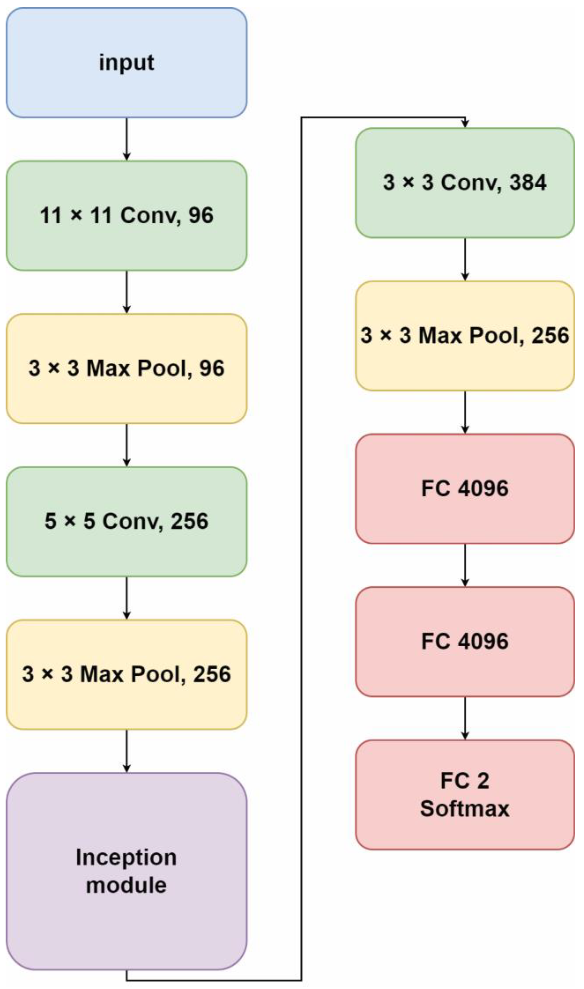
Learning technique transfer involves taking a model that has been pretrained for one task and adapting it to the new task so that the model does not have to be retrained entirely. This reduces the training time. The proposed model was developed to transfer learning and improve AlexNet by removing the fourth and fifth convolution layers from the original AlexNet Model and adding the GoogLeNet inception module layer. The proposed model consists of an image input size of 227 × 227 × 3 pixels, three convolution layers, one inception module, and three fully connected layers. The first convolution layer consists of 96 filters with a filter size of 11 × 11, ReLU, and a max pooling size of 3 × 3. The second convolution layer consists of 256 filters with a filter size of 5 × 5, ReLU, and a max pooling size of 3 × 3. The third layer is the inception module, as shown in
Figure 9. The fourth convolution layer consists of 384 filters with a filter size of 3 × 3, ReLU, and a max pooling size of 3 × 3. The proposed architecture is shown in
Figure 10.
3.2. Mushroom Dataset
The mushroom dataset used in this research included 5 species, 623 images, and an image size of 227 × 227 × 3 pixels. It was divided into two parts. The mushroom data were composed of poisonous and edible mushrooms including the edible types
Amanita citrina (A),
Russula delica (B), and
Phaeogyroporus portentosus (C) and the poisonous types
Inocybe rimosa (D) and
Amanita phalloides (E). The data are presented in
Table 2 and shown in
Figure 11.
Deep learning is a highly accurate method because it uses a large dataset for training; however, if the size of the dataset used in the training is insufficient, unreliable answers can be produced. Therefore, data augmentation is used to increase the amount of data used in training in order to avoid overfitting and ensure the model’s accuracy [
39].
From the mushroom dataset of 623 images, the authors generated a dataset containing 2000 images and divided it into 10 equal groups; these were used in training and testing based on the K-fold cross-validation method, as shown in
Table 3. The dataset was divided into training and test sets using a ratio of 90:10 [
40].
3.3. Confusion Matrix
Before implementing a model, it is necessary to measure its performance to determine whether it is effective enough to be developed or used. A confusion matrix is a tool that describes the performance results for the predictions made by models built with machine learning. The authors measured accuracy using Equation (3), precision using Equation (4), recall using Equation (5), and the F1 score using Equation (2) as the standard metrics to evaluate the results. The Confusion matrix is shown in
Figure 12.
TP indicates a True Positive, where the prediction matched with what happened and the event was true.
TN indicates a True Negative, where the prediction matched what happened and the event was not true.
FP indicates a False Positive, where the prediction did not match what happened and the event was true.
FN indicates a False Negative, where the prediction did not match what happened and the event was not true.
4. Discussion
The mushroom dataset containing 2000 images was divided into two sets: a poisonous mushroom set containing 527 images and an edible mushroom set containing 1473 images. The dataset was divided into training and test sets in a ratio of 90:10.
4.1. Mushroom Classification Using the CNN
As is shown in
Table 4, in training, each architecture used a learning rate = 0.001, MaxEpochs = 10, MiniBatchSize = 40, and was processed with a single GPU.
Figure 13 shows the training results and validation test accuracy for each model. As shown in
Figure 13a, AlexNet achieved a stable training accuracy after 160 iterations with an average training accuracy of 99.60%. As shown in
Figure 13b, GoogLeNet achieved a stable training accuracy after 125 iterations with an average training accuracy of 99.70%. As can be seen in
Figure 13c, ResNet-50 achieved a stable training accuracy after 40 iterations with an average training accuracy of 99.55%. In addition,
Figure 13d shows that the proposed model achieved stable training accuracy after 340 iterations with an average training accuracy of 97.95%.
As can be observed in
Table 5, ResNet-50 was found to be the most accurate model with an accuracy of 99.50%, a precision of 99.33%, a recall of 100%, an F1 score of 99.66%, and a training time of 5 min 50 s. This was followed by GoogLeNet with an accuracy of 99.50%, a precision of 99.35%, a recall of 100%, an F1 score of 99.97%, and a training time of 2 min 20 s. Next came AlexNet with an accuracy of 99.00%, a precision of 98.61%, a recall of 100%, an F1 score of 99.30%, and a training time of 1 min 42 s. Finally, the proposed model exhibited an accuracy of 98.50%, a precision of 99.39%, a recall of 98.79%, an F1 score of 99.09%, and a training time of 1 min 10 s. The confusion matrix accuracy is shown in
Figure 14.
4.2. Mushroom Classification Using the R-CNN
As is shown in
Table 6, in training, each architecture utilized a learning rate of 0.001, MaxEpochs = 1, MiniBatchSize = 20, and was processed with a single GPU. An example of detection using the R-CNN is shown in
Figure 15.
As is shown in
Table 7, ResNet-50 was found to be the most accurate model with an accuracy of 96.50%, precision of 100%, recall of 95.24%, an F1 score of 97.56%, and a training time of 13 min 44 s. GoogLeNet followed with an accuracy of 96.50%; 99.30% precision; 95.92% recall; an F1 score of 97.58%; and a training time of 7 min 28 s. Next, the proposed model had an accuracy of 95.50%; 94.59% precision; 99.29% recall; an F1 score of 96.89%; and a training time of 4 min 37 s. Finally, AlexNet demonstrated an accuracy of 95.00%; 97.24% precision; 95.92% recall; an F1 score of 96.58%; and a training time of 5 min 7 s. The confusion matrix accuracy is shown in
Figure 16.
5. Conclusions
In this study, a method for the classification of edible and poisonous mushrooms was proposed. The experimental results show that the proposed model can accurately classify poisonous and edible mushrooms and can shorten training and testing times. Moreover, the testing time and accuracy of the proposed model were compared with three pretrained models: AlexNet, ResNet-50, and GoogLeNet.
In the mushroom classification experiment carried out using CNN, the proposed model provided the result the fastest, in 1 min 10 s, while maintaining an accuracy level of 98.50%. This was less accurate than ResNet-50, and GoogLeNet at 99.50%; however, they took 5 min 50 s and 2 min 20 s, respectively.
In the mushroom detection experiment using R-CNN, ResNet-50 also demonstrated the highest accuracy level of 96.50%, but took the longest time for training, i.e., 13 min 44 s. The proposed model again produced the training results the fastest in only 4 min 37 s, with an accuracy of 95.50%. However, there was a different of 1% in the accuracy levels of ResNet-50 and the proposed model, and ResNet-50 took 9 min 7 s to obtain a result.
In the future, more varieties of mushrooms and different backgrounds can be added to the dataset to provide greater coverage and develop improved applications for mushroom classification.
Author Contributions
Conceptualization, W.K. and U.K.; methodology, W.K.; software, W.K.; validation, W.K., U.K. and S.B.; formal analysis, W.K.; investigation, S.B.; resources, S.B.; data curation, S.B.; writing—original draft preparation, W.K. and U.K.; writing—review and editing, W.K., U.K. and S.B.; visualization, W.K.; supervision, U.K.; project administration, U.K.; funding acquisition, U.K. All authors have read and agreed to the published version of the manuscript.
Funding
This research was funded by the research capability enhancement program through a graduate student scholarship at the Faculty of Science, Khon Kaen University (No. SCG-2018-3).
Institutional Review Board Statement
Not applicable.
Informed Consent Statement
Not applicable.
Data Availability Statement
Acknowledgments
The authors would like to thank the Department of Microbiology for their support with the data collection and the Applied Intelligence & Data Analytics Laboratory, College of Computing, Khon Kaen University for providing the research location and equipment used in this study.
Conflicts of Interest
The authors declare no conflict of interest.
References
- Ria, N.J.; Badhon, S.M.S.I.; Khushbu, S.A.; Akter, S.; Hossain, S.A. State of art Research in Edible and Poisonous Mushroom Recognition. In Proceedings of the International Conference on Computing Communication and Networking Technologies, Kharagpur, India, 6–8 July 2021; pp. 1–5. [Google Scholar]
- Wibowo, A.; Rahayu, Y.; Riyanto, A.; Hidayatulloh, T. Classification algorithm for edible mushroom identification. In Proceedings of the International Conference on Information and Communications Technology, Yogyakarta, Indonesia, 6–7 March 2018; pp. 250–253. [Google Scholar]
- Mešić, A.; Šamec, D.; Jadan, M.; Bahun, V.; Tkalčec, Z. Integrated morphological with molecular identification and bioactive compounds of 23 Croatian wild mushrooms samples. Food Biosci. 2020, 37, 100720. [Google Scholar] [CrossRef]
- Chitayae, N.; Sunyoto, A. Performance Comparison of Mushroom Types Classification Using K-Nearest Neighbor Method and Decision Tree Method. In Proceedings of the International Conference on Information and Communications Technology, Yogyakarta, Indonesia, 24–25 November 2020; pp. 308–313. [Google Scholar]
- Zahan, N.; Hasan, M.Z.; Malek, M.A.; Reya, S.S. A Deep Learning-Based Approach for Edible, Inedible and Poisonous Mushroom Classification. In Proceedings of the International Conference on Information and Communication Technology for Sustainable Development, Dhaka, Bangladesh, 27–28 February 2021; pp. 440–444. [Google Scholar]
- Khan, S.; Ahmed, E.; Javed, M.H.; Shah, S.A.A.; Ali, S.U. Transfer Learning of a Neural Network Using Deep Learning to Perform Face Recognition. In Proceedings of the International Conference on Electrical, Communication and Computer Engineering, Swat, Pakistan, 24–25 July 2019; pp. 1–5. [Google Scholar]
- Lin, M.; Zhang, Z.; Zheng, W. A Small Sample Face Recognition Method Based on Deep Learning. In Proceedings of the IEEE 20th International Conference on Communication Technology, Nanning, China, 28–31 October 2020; pp. 1394–1398. [Google Scholar]
- Rahman, A.; Islam, M.; Mahdee, G.M.S.; Kabir, W.U. Improved Segmentation Approach for Plant Disease Detection. In Proceedings of the International Conference on Advances in Science, Engineering and Robotics Technology, Dhaka, Bangladesh, 3–5 May 2019; pp. 1–5. [Google Scholar]
- Militante, S.V.; Gerardo, B.D.; Dionisio, N.V. Plant Leaf Detection and Disease Recognition using Deep Learning. In Proceedings of the IEEE Eurasia Conference on IOT, Communication and Engineering, Yunlin, Taiwan, 3–6 October 2019; pp. 579–582. [Google Scholar]
- Alhabshee, S.M.; bin Shamsudin, A.U. Deep Learning Traffic Sign Recognition in Autonomous Vehicle. In Proceedings of the IEEE Student Conference on Research and Development, Batu Pahat, Malaysia, 27–29 September 2020; pp. 438–442. [Google Scholar]
- Tarmizi, I.A.; Aziz, A.A. Vehicle Detection Using Convolutional Neural Network for Autonomous Vehicles. In Proceedings of the International Conference on Intelligent and Advanced System, Kuala Lumpur, Malaysia, 13–14 August 2018; pp. 1–5. [Google Scholar]
- Dominguez-Catena, I.; Paternain, D.; Galar, M. A Study of OWA Operators Learned in Convolutional Neural Networks. Appl. Sci. 2021, 11, 7195. [Google Scholar] [CrossRef]
- Lee, C.; Hong, S.; Hong, S.; Kim, T. Performance analysis of local exit for distributed deep neural networks over cloud and edge computing. ETRI J. 2020, 5, 658–668. [Google Scholar] [CrossRef]
- Sajanraj, T.D.; Beena, M. Indian Sign Language Numeral Recognition Using Region of Interest Convolutional Neural Network. In Proceedings of the International Conference on Inventive Communication and Computational Technologies, Coimbatore, India, 20–21 April 2018; pp. 636–640. [Google Scholar]
- Naranjo-Torres, J.; Mora, M.; Hernández-García, R.; Barrientos, R.J.; Fredes, C.; Valenzuela, A. A Review of Convolutional Neural Network Applied to Fruit Image Processing. Appl. Sci. 2020, 10, 3443. [Google Scholar] [CrossRef]
- Dong, J.; Zheng, L. Quality Classification of Enoki Mushroom Caps Based on CNN. In Proceedings of the IEEE 4th International Conference on Image, Vision and Computing, Xiamen, China, 5–7 July 2019; pp. 450–454. [Google Scholar]
- Mostafa, A.M.; Kumar, S.A.; Meraj, T.; Rauf, H.T.; Alnuaim, A.A.; Alkhayyal, M.A. Guava Disease Detection Using Deep Convolutional Neural Networks: A Case Study of Guava Plants. Appl. Sci. 2022, 12, 239. [Google Scholar] [CrossRef]
- Arora, D.; Garg, M.; Gupta, M. Diving deep in Deep Convolutional Neural Network. In Proceedings of the International Conference on Advances in Computing, Communication Control and Networking, Greater Noida, India, 18–19 December 2020; pp. 749–751. [Google Scholar]
- Guo, T.; Dong, J.; Li, H.; Gao, Y. Simple convolutional neural network on image classification. In Proceedings of the International Conference on Big Data Analysis, Beijing, China, 10–12 March 2017; pp. 721–724. [Google Scholar]
- Hsiao, T.-Y.; Chang, Y.-C.; Chiu, C.-T. Filter-based Deep-Compression with Global Average Pooling for Convolutional Networks. In Proceedings of the 2018 IEEE International Workshop on Signal Processing Systems, Cape Town, South Africa, 21–24 October 2018; pp. 247–251. [Google Scholar]
- Gholamalinezhad, H.; Khosravi, H. Pooling Methods in Deep Neural Networks, a Review. arXiv 2020, arXiv:2009.07485. [Google Scholar]
- Nirthika, R.; Manivannan, S.; Ramanan, A. An experimental study on convolutional neural network-based pooling techniques for the classification of HEp-2 cell images. In Proceedings of the 2021 10th International Conference on Information and Automation for Sustainability, Negambo, Sri Lanka, 11–13 August 2021; pp. 281–286. [Google Scholar]
- Momeny, M.; Neshat, A.A.; Gholizadeh, A.; Jafarnezhad, A.; Rahmanzadeh, E.; Marhamati, M.; Moradi, B.; Ghafoorifar, A.; Zhang, Y.-D. Greedy Autoaugment for classification of mycobacterium tuberculosis image via generalized deep CNN using mixed pooling based on minimum square rough entropy. Comput. Biol. Med. 2022, 141, 105175. [Google Scholar] [CrossRef] [PubMed]
- Zheng, S. Network Intrusion Detection Model Based on Convolutional Neural Network. In Proceedings of the Advanced Information Technology, Electronic and Automation Control Conference, Chongqing, China, 12–14 March 2021; pp. 634–637. [Google Scholar]
- Kido, S.; Hirano, Y.; Hashimoto, N. Detection and Classification of Lung Abnormalities by Use of Convolutional Neural Network (CNN) and Regions with CNN Features (R-CNN). In Proceedings of the International Workshop on Advanced Image Technology, Chiang Mai, Thailand, 7–9 January 2018. [Google Scholar]
- Yanagisawa, H.; Yamashita, T.; Watanabe, H. A Study on Object Detection Method from Manga Images using CNN. In Proceedings of the International Workshop on Advanced Image Technology, Chiang Mai, Thailand, 7–9 January 2018. [Google Scholar]
- Sun, S.; Zhang, T.; Li, Q.; Wang, J.; Zhang, W.; Wen, Z.; Tang, Y. Fault Diagnosis of Conventional Circuit Breaker Contact System Based on Time–Frequency Analysis and Improved AlexNet. IEEE Trans. Instrum. Meas. 2021, 70, 1–12. [Google Scholar] [CrossRef]
- Beeharry, Y.; Bassoo, V. Performance of ANN and AlexNet for weed detection using UAV-based images. In Proceedings of the International Conference on Emerging Trends in Electrical, Electronic and Communications Engineering, Balaclava, Mauritius, 25–27 November 2020; pp. 163–167. [Google Scholar]
- Wan, S.; Liang, Y.; Zhang, Y. Deep convolutional neural networks for diabetic retinopathy detection by image classification. Comput. Electr. Eng. 2018, 72, 274–282. [Google Scholar] [CrossRef]
- Tariq, H.; Rashid, M.; Javed, A.; Zafar, E.; Alotaibi, S.S.; Zia, M.Y.I. Performance Analysis of Deep-Neural-Network-Based Automatic Diagnosis of Diabetic Retinopathy. Sensors 2022, 22, 205. [Google Scholar] [CrossRef] [PubMed]
- Rahmathunneesa, A.P.; Muneer, K.V.A. Performance Analysis of Pre-trained Deep Learning Networks for Brain Tumor Categorization. In Proceedings of the International Conference on Advances in Computing and Communication, Kochi, India, 6–8 November 2019; pp. 253–257. [Google Scholar]
- Mukti, I.Z.; Biswas, D. Transfer Learning Based Plant Diseases Detection Using ResNet50. In Proceedings of the International Conference on Electrical Information and Communication Technology, Khulna, Bangladesh, 20–22 December 2019; pp. 1–6. [Google Scholar]
- Zhao, X.; Li, K.; Li, Y.; Ma, J.; Zhang, L. Identification method of vegetable diseases based on transfer learning and attention mechanism. Comput. Electron. Agric. 2022, 6, 106703. [Google Scholar] [CrossRef]
- Fu, Y.; Song, J.; Xie, F.; Bai, Y.; Zheng, X.; Gao, P.; Wang, Z.; Xie, S. Circular Fruit and Vegetable Classification Based on Optimized GoogLeNet. IEEE Access 2021, 6, 113599–113611. [Google Scholar]
- Balagourouchetty, L.; Pragatheeswaran, J.K.; Pottakkat, B.; Ramkumar, G. GoogLeNet-Based Ensemble FCNet Classifier for Focal Liver Lesion Diagnosis. IEEE J. Biomed. Health Inform. 2020, 6, 1686–1694. [Google Scholar] [CrossRef] [PubMed]
- Jasitha, P.; Dileep, M.R.; Divya, M. Venation Based Plant Leaves Classification Using GoogLeNet and VGG. In Proceedings of the International Conference on Recent Trends on Electronics, Information, Communication & Technology, Bangalore, India, 17–18 May 2019; pp. 715–719. [Google Scholar]
- Haritha, D.; Swaroop, N.; Mounika, M. Prediction of COVID-19 Cases Using CNN with X-rays. In Proceedings of the International Conference on Computing, Communication and Security, Patna, India, 14–16 October 2020; pp. 1–6. [Google Scholar]
- Lin, C.; Li, Y.; Liu, H.; Huang, Q.; Li, Y.; Cai, Q. Power Enterprise Asset Estimation Algorithm Based on Improved GoogLeNet. In Proceedings of the 2020 Chinese Automation Congress, Shanghai, China, 6–8 November 2020; pp. 883–887. [Google Scholar]
- Xu, P.; Tan, Q.; Zhang, Y.; Zha, X.; Yang, S.; Yang, R. Research on Maize Seed Classification and Recognition Based on Machine Vision and Deep Learning. Agriculture 2022, 12, 232. [Google Scholar] [CrossRef]
- Firdaus, N.M.; Chahyati, D.; Fanany, M.I. Tourist Attractions Classification using ResNet. In Proceedings of the International Conference on Advanced Computer Science and Information Systems, Yogyakarta, Indonesia, 27–28 October 2018; pp. 429–433. [Google Scholar]
Figure 1.
Convolutional neural network architecture.
Figure 1.
Convolutional neural network architecture.
Figure 2.
Convolution layer.
Figure 2.
Convolution layer.
Figure 3.
Example of a pooling layer showing both max pooling and average pooling.
Figure 3.
Example of a pooling layer showing both max pooling and average pooling.
Figure 4.
Region convolutional neural network architecture.
Figure 4.
Region convolutional neural network architecture.
Figure 5.
AlexNet architecture.
Figure 5.
AlexNet architecture.
Figure 6.
Bottleneck building blocks.
Figure 6.
Bottleneck building blocks.
Figure 7.
ResNet-50 architecture.
Figure 7.
ResNet-50 architecture.
Figure 8.
GoogLeNet architecture.
Figure 8.
GoogLeNet architecture.
Figure 9.
Inception module.
Figure 9.
Inception module.
Figure 10.
Proposed architecture.
Figure 10.
Proposed architecture.
Figure 11.
Examples of mushroom images: (A1–A8) Amanita citrina; (B1–B8) Russula delica; (C1–C8) Phaeogyroporus portentosus; (D1–D8) Inocybe rimosa; (E1–E8) Amanita phalloides.
Figure 11.
Examples of mushroom images: (A1–A8) Amanita citrina; (B1–B8) Russula delica; (C1–C8) Phaeogyroporus portentosus; (D1–D8) Inocybe rimosa; (E1–E8) Amanita phalloides.
Figure 12.
Confusion matrix.
Figure 12.
Confusion matrix.
Figure 13.
Training results: (a) AlexNet; (b) GoogLeNet; (c) ResNet-50; (d) proposed model.
Figure 13.
Training results: (a) AlexNet; (b) GoogLeNet; (c) ResNet-50; (d) proposed model.
Figure 14.
The confusion matrix of the CNN analysis: (a) proposed model; (b) AlexNet; (c) GoogLeNet; (d) ResNet-50.
Figure 14.
The confusion matrix of the CNN analysis: (a) proposed model; (b) AlexNet; (c) GoogLeNet; (d) ResNet-50.
Figure 15.
The object detection prediction results: (a) Amanita citrina; (b) Inocybe rimosa; (c) Amanita phalloides; (d) Russula delica; (e) Phaeogyroporus portentosus.
Figure 15.
The object detection prediction results: (a) Amanita citrina; (b) Inocybe rimosa; (c) Amanita phalloides; (d) Russula delica; (e) Phaeogyroporus portentosus.
Figure 16.
The confusion matrix for the R-CNN analysis: (a) proposed model; (b) AlexNet; (c) GoogLeNet; (d) ResNet-50.
Figure 16.
The confusion matrix for the R-CNN analysis: (a) proposed model; (b) AlexNet; (c) GoogLeNet; (d) ResNet-50.
Table 1.
AlexNet Architecture Convolution Layer.
Table 1.
AlexNet Architecture Convolution Layer.
| Layer | Filters | Filter Size | Strides |
|---|
| 1 | 96 | 11 × 11 | 4 |
| 2 | 256 | 5 × 5 | 1 |
| 3 | 384 | 3 × 3 | 1 |
| 4 | 384 | 3 × 3 | 1 |
| 5 | 256 | 3 × 3 | 1 |
Table 2.
Mushroom dataset.
Table 2.
Mushroom dataset.
| Edible Mushrooms | Poisonous Mushrooms |
|---|
| A | B | C | D | E |
| 248 | 88 | 155 | 76 | 56 |
Table 3.
K-Folds cross-validation.
Table 3.
K-Folds cross-validation.
| Group | Amount | Group | Amount |
|---|
| 1 | 200 | 6 | 200 |
| 2 | 200 | 7 | 200 |
| 3 | 200 | 8 | 200 |
| 4 | 200 | 9 | 200 |
| 5 | 200 | 10 | 200 |
Table 4.
CNN parameters used in training.
Table 4.
CNN parameters used in training.
| Parameters | Architecture |
|---|
| AlexNet | ResNet-50 | GoogLeNet | Proposed Model |
|---|
| Learning rate | 0.001 | 0.001 | 0.001 | 0.001 |
| MaxEpochs | 10 | 10 | 10 | 10 |
| MiniBatchSize | 40 | 40 | 40 | 40 |
Table 5.
Analysis of the CNN test results.
Table 5.
Analysis of the CNN test results.
| Architecture | Accuracy | Time |
|---|
| ResNet-50 | 99.50% | 5.50 min |
| GoogLeNet | 99.50% | 2.20 min |
| AlexNet | 99.00% | 1.42 min |
| Proposed Model | 98.50% | 1.10 min |
Table 6.
R-CNN parameters used in training.
Table 6.
R-CNN parameters used in training.
| Parameters | Architecture |
|---|
| AlexNet | ResNet-50 | GoogLeNet | Proposed Model |
|---|
| Learning rate | 0.001 | 0.001 | 0.001 | 0.001 |
| MaxEpochs | 1 | 1 | 1 | 1 |
| MiniBatchSize | 20 | 20 | 20 | 20 |
Table 7.
Analysis of the R-CNN test results.
Table 7.
Analysis of the R-CNN test results.
| Architecture | Accuracy | Time |
|---|
| ResNet-50 | 96.50% | 13.44 min |
| GoogLeNet | 96.50% | 7.28 min |
| Proposed Model | 95.50% | 4.37 min |
| AlexNet | 95.00% | 5.07 min |
| Publisher’s Note: MDPI stays neutral with regard to jurisdictional claims in published maps and institutional affiliations. |
© 2022 by the authors. Licensee MDPI, Basel, Switzerland. This article is an open access article distributed under the terms and conditions of the Creative Commons Attribution (CC BY) license (https://creativecommons.org/licenses/by/4.0/).


