
Air Flow Study around Isolated Cubical Building in the City of Athens under Various Climate Conditions

 ,
,  ,
, 
Abstract
:1. Introduction
2. Configuration and Pollutant Dispersion Modelling
2.1. Problem Configuration
2.2. Governing Equations
2.3. Urban Surface Model (USM) of the PALM Model System
3. Initial and Boundary Conditions
4. Nested Computational Grid
5. Numerical Details
6. Results and Discussion
7. Conclusions
Author Contributions
Funding
Institutional Review Board Statement
Informed Consent Statement
Data Availability Statement
Acknowledgments
Conflicts of Interest
References
- Sini, J.-F.; Anquetin, S.; Mestayer, P.G. Pollutant dispersion and thermal effects in urban street canyons. Atmos. Environ. 1996, 30, 2659–2677. [Google Scholar] [CrossRef]
- Barlow, F.J.; Harman, I.N.; Belcher, S.E. Scalar fluxes from urban street canyons. Part I: Laboratory simulation. Bound. Layer Meteorol. 2004, 113, 369–385. [Google Scholar] [CrossRef]
- Rotach, M.W.; Gryning, S.E.; Batchvarova, E.; Christen, A.; Vogt, R. Pollutant dispersion close to an urban surface—The BUBBLE tracer experiment. Meteorol. Atmos. Phys. 2004, 87, 39–56. [Google Scholar] [CrossRef]
- Vasilopoulos, K.; Mentzos, M.; Sarris, I.E.; Tsoutsanis, P. Computational Assessment of the Hazardous Release Dispersion from a Diesel Pool Fire in a Complex Building’s Area. Computation 2018, 6, 65. [Google Scholar] [CrossRef] [Green Version]
- Kim, D.J.; Lee, D.I.; Kim, J.J.; Park, M.S.; Lee, S.H. Development of a Building-Scale Meteorological Prediction System Including a Realistic Surface Heating. Atmosphere 2020, 11, 67. [Google Scholar] [CrossRef] [Green Version]
- Kovar-Panskus, A.; Louka, P.; Sini, J.F.; Savory, E.; Czech, M.; Abdelqari, A.; Mestayer, P.G.; Toy, N. Influence of Geometry on the Mean Flow within Urban Street Canyons—A Comparison of Wind Tunnel Experiments and Numerical Simulations. Water Air Soil Pollut. Focus 2002, 2, 365–380. [Google Scholar] [CrossRef]
- Dallman, A.; Magnusson, S.; Britter, R.; Norford, L.; Entekhabi, D.; Fernando, H.J. Conditions for thermal circulation in urban street canyons. Build. Environ. 2014, 80, 184–191. [Google Scholar] [CrossRef]
- Madalozzo DM, S.; Braun, A.L.; Awruch, A.M.; Morsch, I.B. Numerical simulation of pollutant dispersion in street canyons: Geometric and thermal effects. Appl. Math. Model. 2014, 38, 5883–5909. [Google Scholar] [CrossRef]
- Chatzimichailidis, A.E.; Argyropoulos, C.D.; Assael, M.J.; Kakosimos, K.E. Implicit Definition of Flow Patterns in Street Canyons—Recirculation Zone—Using Exploratory Quantitative and Qualitative Methods. Atmosphere 2019, 10, 794. [Google Scholar] [CrossRef] [Green Version]
- Chatzimichailidis, A.; Assael, M.; Ketzel, M.; Kakosimos, K.E. Modelling the Recirculation Zone in street canyons with different aspect ratios, using CFD simulation. In Proceedings of the 17th International Conference on Harmonisation within Atmospheric Dispersion Modelling for Regulatory Purposes, Budapest, Hungary, 9–12 May 2016. [Google Scholar]
- Ming, T.; Fang, W.; Peng, C.; Cai, C.; de Richter, R.; Ahmadi, M.H.; Wen, Y. Impacts of Traffic Tidal Flow on Pollutant Dispersion in a Non-Uniform Urban Street Canyon. Atmosphere 2018, 9, 82. [Google Scholar] [CrossRef] [Green Version]
- Chatzimichailidis, A.E.; Argyropoulos, C.D.; Assael, M.J.; Kakosimos, K.E. Qualitative and Quantitative Investigation of Multiple Large Eddy Simulation Aspects for Pollutant Dispersion in Street Canyons Using OpenFOAM. Atmosphere 2019, 10, 17. [Google Scholar] [CrossRef] [Green Version]
- Pisello, A.L.; Pignatta, G.; Castaldo, V.L.; Cotana, F. The Impact of Local Microclimate Boundary Conditions on Building Energy Performance. Sustainability 2015, 7, 9207–9230. [Google Scholar] [CrossRef] [Green Version]
- Blanken, P.D.; Barry, R.G. (Eds.) Urban Climates. In Microclimate and Local Climate; Cambridge University Press: Cambridge, UK, 2016; pp. 243–260. [Google Scholar] [CrossRef]
- Kim, J.-J.; Baik, J.-J. A Numerical Study of Thermal Effects on Flow and Pollutant Dispersion in Urban Street Canyons. J. Appl. Meteorol. 1999, 38, 1249–1261. [Google Scholar] [CrossRef]
- Baik, J.-J.; Kim, J.-J.; Fernando, H. A CFD Model for Simulating Urban Flow and Dispersion. J. Appl. Meteorol. 2003, 42, 1636–1648. [Google Scholar] [CrossRef]
- Kwak, K.H.; Baik, J.J.; Lee, S.H.; Ryu, Y.H. Computational Fluid Dynamics Modelling of the Diurnal Variation of Flow in a Street Canyon. Bound. Layer Meteorol. 2011, 141, 77–92. [Google Scholar] [CrossRef]
- Park, S.B.; Baik, J.J.; Raasch, S.; Letzel, M.O. A Large-Eddy Simulation Study of Thermal Effects on Turbulent Flow and Dispersion in and above a Street Canyon. J. Appl. Meteorol. Climatol. 2012, 51, 829–841. [Google Scholar] [CrossRef]
- Santiago, J.; Krayenhoff, E.; Martilli, A. Flow simulations for simplified urban configurations with microscale distributions of surface thermal forcing. Urban Clim. 2014, 9, 115–133. [Google Scholar] [CrossRef]
- Nazarian, N.; Kleissl, J. CFD simulation of an idealized urban environment: Thermal effects of geometrical characteristics and surface materials. Urban Clim. 2015, 12, 141–159. [Google Scholar] [CrossRef]
- Nazarian, N.; Kleissl, J. Realistic solar heating in urban areas: Air exchange and street-canyon ventilation. Build. Environ. 2016, 95, 75–93. [Google Scholar] [CrossRef] [Green Version]
- Resler, J.; Krč, P.; Belda, M.; Juruš, P.; Benešová, N.; Lopata, J.; Kanani-Sühring, F. PALM-USM v1.0: A new urban surface model integrated into the PALM large-eddy simulation model. Geosci. Model Dev. 2017, 10, 3635–3659. [Google Scholar] [CrossRef] [Green Version]
- Lee, D.-I.; Woo, J.-W.; Lee, S.-H. An analytically based numerical method for computing view factors in real urban environments. Theor. Appl. Climatol. 2018, 131, 445–453. [Google Scholar] [CrossRef]
- Oke, T.R. The energetic basis of the urban heat island. Q. J. R. Meteorol. Soc. 1982, 108, 1–24. [Google Scholar] [CrossRef]
- Tam, B.Y.; Gough, W.A.; Mohsin, T. The impact of urbanization and the urban heat island effect on day to day temperature variation. Urban Clim. 2015, 12, 1–10. [Google Scholar] [CrossRef]
- Brown, M. Urban Parameterizations for Mesoscale Meteorological Models. In Mesoscale Atmospheric Dispersion; WIT Press: England, UK, 2000; pp. 193–255. [Google Scholar]
- Fisher, B.; Kukkonen, J.; Piringer, M.; Rotach, M.W.; Schatzmann, M. Meteorology applied to urban air pollution problems: Concepts from COST 715. Atmos. Chem. Phys. 2006, 6, 555–564. [Google Scholar] [CrossRef] [Green Version]
- Gronemeier, T.; Raasch, S.; Ng, E. Effects of Unstable Stratification on Ventilation in Hong Kong. Atmosphere 2017, 8, 168. [Google Scholar] [CrossRef] [Green Version]
- Wang, W.; Xu, Y.; Ng, E. Large-eddy simulations of pedestrian-level ventilation for assessing a satellite-based approach to urban geometry generation. Graph. Models 2018, 95, 29–41. [Google Scholar] [CrossRef]
- Pfafferott, J.; Rißmann, S.; Sühring, M.; Kanani-Sühring, F.; Maronga, B. Building indoor model in PALM model system 6.0: Indoor climate, energy demand, and the interaction between buildings and the urban climate. Geosci. Model Dev. Discuss. 2020, 14, 199. [Google Scholar] [CrossRef]
- Resler, J.; Eben, K.; Geletič, J.; Krč, P.; Rosecký, M.; Sühring, M.; Belda, M.; Fuka, V.; Halenka, T.; Huszár, P.; et al. Validation of the PALM model system 6.0 in real urban environment; case study of Prague-Dejvice, Czech Republic. Geosci. Model Dev. Discuss. 2020, 14, 175. [Google Scholar] [CrossRef]
- Allwine, K.J.; Leach, M.J.; Stockham, L.W.; Shinn, J.S.; Hosker, R.P.; Bowers, J.F.; Pace, J.C. Overview of Joint Urban 2003: An atmospheric dispersion study in Oklahoma City. In Proceedings of the 84th AMS Annual Meeting, Seattle, WA, USA, 11–15 January 2004. [Google Scholar]
- Park, M.S.; Park, S.H.; Chae, J.H.; Choi, M.H.; Song, Y.; Kang, M.; Roh, J.W. High-resolution urban observation network for user-specific meteorological information service in the Seoul Metropolitan Area, South Korea. Atmos. Meas. Tech. 2017, 10, 1575–1594. [Google Scholar] [CrossRef]
- Gowardhan, A.A.; Brown, M.J.; Pardyjak, E.R. Evaluation of a fast response pressure solver for flow around an isolated cube. Environ. Fluid Mech. 2010, 10, 311–328. [Google Scholar] [CrossRef]
- Lim, H.C.; Thomas, T.G.; Castro, I.P. Flow around a cube in a turbulent boundary layer: LES and experiment. J. Wind. Eng. Ind. Aerodyn. 2009, 97, 96–109. [Google Scholar] [CrossRef] [Green Version]
- Yazid, A.W.M.; Sidik, N.A.C. Prediction of the Flow around a Surface-Mounted Cube Using Two-Equation Turbulence Models. Appl. Mech. Mater. 2013, 315, 438–442. [Google Scholar] [CrossRef]
- Mochida, A.; Tominaga, Y.; Murakami, S.; Yoshie, R.; Ishihara, T.; Ooka, R. Comparison of various k-ε models and DSM applied to flow around a high-rise building—Report on AIJ cooperative project for CFD prediction of wind environment. Wind. Struct. 2002, 5, 227–244. [Google Scholar] [CrossRef] [Green Version]
- Dogan, S.; Yagmur, S.; Goktepeli, I.; Ozgoren, M. Assessment of turbulence models for flow around a surface-mounted cube. Int. J. Mech. Eng. Robot. Res. 2017, 6, 237–241. [Google Scholar] [CrossRef] [Green Version]
- Brown, M.J.; Lawson, R.E.; Decroix, D.S.; Lee, R.L. Mean flow and turbulence measurement around a 2-darray of buildings in a wind tunnel. In Proceedings of the AMS 11th Joint Conference on the Applications of Air Pollution Meteorology, Long Beach, CA, USA, 9–13 January 2000. Report LA-UR-99-5395. [Google Scholar]
- Brown, M.J. Comparison of Centerline Velocity Measurements Obtained around 1d and 3d Building Arrays in a Wind Tunnel. In Proceedings of the International Society of Environmental Hydraulics Conference, Tempe, AZ, USA, 5–8 December 2001. [Google Scholar]
- Uehara, K.; Murakami, S.; Oikawa, S.; Wakamatsu, S. Wind tunnel experiments on how thermal stratification affects flow in and above urban street canyons. Atmos. Environ. 2000, 34, 1553–1562. [Google Scholar] [CrossRef]
- Tseng, Y.-H.; Meneveau, C.; Parlange, M.B. Modeling Flow around Bluff Bodies and Predicting Urban Dispersion Using Large Eddy Simulation. Environ. Sci. Technol. 2006, 40, 2653–2662. [Google Scholar] [CrossRef] [Green Version]
- Richards, P.J.; Hoxey, R.P.; Short, L.J. Wind pressures on a 6m cube. J. Wind. Eng. Ind. Aerodyn. 2001, 89, 1553–1564. [Google Scholar] [CrossRef]
- Richards, P.J.; Hoxey, R.P.; Connell, B.D.; Lander, D.P. Wind-tunnel modelling of the Silsoe Cube. J. Wind. Eng. Ind. Aerodyn. 2007, 95, 1384–1399. [Google Scholar] [CrossRef]
- Zheng, X.; Montazeri, H.; Blocken, B. CFD simulations of wind flow and mean surface pressure for buildings with balconies: Comparison of RANS and LES. Build. Environ. 2020, 173, 106747. [Google Scholar] [CrossRef]
- Franke, J.; Baklanov, A. Best Practice Guideline for the CFD Simulation of Flows in the Urban Environment: COST Action 732 Quality Assurance and Improvement of Microscale Meteorological Models; Meteorological Institute, University of Hamburg: Hamburg, Germany, 2007. [Google Scholar]
- Tominaga, Y.; Mochida, A.; Yoshie, R.; Kataoka, H.; Nozu, T.; Yoshikawa, M.; Shirasawa, T. AIJ guidelines for practical applications of CFD to pedestrian wind environment around buildings. J. Wind. Eng. Ind. Aerodyn. 2008, 96, 1749–1761. [Google Scholar] [CrossRef]
- Li, W.-W.; Meroney, R. Gas dispersion near a cubical model building. Part II. Concentration fluctuation measurements. J. Wind. Eng. Ind. Aerodyn. 1983, 12, 35–47. [Google Scholar] [CrossRef]
- Saathof, P.J.; Stathopoulos, T.; Dobrescu, M. Effects of model scale in estimating pollutant dispersion near buildings. J. Wind. Eng. Ind. Aerodyn. 1995, 54–55, 549–559. [Google Scholar] [CrossRef]
- Bird, R.B.; Stewart, W.E.; Lightfoot, E.N. Transport Phenomena; Wiley: Hoboken, NJ, USA, 2006. [Google Scholar]
- Krayenhoff, E.S.; Voogt, J.A. A microscale three-dimensional urban energy balance model for studying surface temperatures. Bound. Layer Meteorol. 2007, 123, 433–461. [Google Scholar] [CrossRef]
- Monin, A.S.; Obukhov, A.M. Basic laws of turbulent mixing in the surface layer of the atmosphere. Contrib. Geophys. Inst. Acad. Sci. USSR 1954, 24, 163–187. [Google Scholar]
- Obukhov, A.M. Turbulence in an atmosphere with a non-uniform temperature. Bound. Layer Meteorol. 1971, 2, 7–29. [Google Scholar] [CrossRef]
- Castro, I.; Robins, A. The flow around a surface-mounted cube in uniform and turbulent streams. J. Fluid Mech. 1977, 79, 307–335. [Google Scholar] [CrossRef]
- Arakawa, A.; Lamb, V.R. Computational Design of the Basic Dynamical Processes of the UCLA General Circulation Model. In Methods in Computational Physics: Advances in Research and Applications; Chang, J., Ed.; Elsevier: Amsterdam, The Netherlands, 1977; pp. 173–265. [Google Scholar] [CrossRef]
- Wicker, L.J.; Skamarock, W.C. Time-Splitting Methods for Elastic Models Using Forward Time Schemes. Mon. Weather. Rev. 2002, 130, 2088–2097. [Google Scholar] [CrossRef]
- Williamson, J.H. Low-storage Runge-Kutta schemes. J. Comput. Phys. 1980, 35, 48–56. [Google Scholar] [CrossRef]
- Deardorff, J.W. Stratocumulus-capped mixed layers derived from a three-dimensional model. Bound. Layer Meteorol. 1980, 18, 495–527. [Google Scholar] [CrossRef]
- Moeng, C.-H.; Wyngaard, J.C. Spectral Analysis of Large-Eddy Simulations of the Convective Boundary Layer. J. Atmos. Sci. 1988, 45, 3573–3587. [Google Scholar] [CrossRef] [Green Version]
- Saiki, E.M.; Moeng, C.-H.; Sullivan, P.P. Large-Eddy Simulation of The Stably Stratified Planetary Boundary Layer. Bound. Layer Meteorol. 2000, 95, 1–30. [Google Scholar] [CrossRef] [Green Version]
- Martinuzzi, R.; Tropea, C. The Flow Around Surface-Mounted, Prismatic Obstacles Placed in a Fully Developed Channel Flow (Data Bank Contribution). J. Fluids Eng. 1993, 115, 85–92. [Google Scholar] [CrossRef]
- Rodi, W. Comparison of LES and RANS calculations of the flow around bluff bodies. J. Wind. Eng. Ind. Aerodyn. 1997, 69, 55–75. [Google Scholar] [CrossRef]
- Hoxey, R.P.; Richards, P.; Short, J.L. A 6 m cube in an atmospheric boundary layer flow—Part 1. Full-scale and wind-tunnel results. Wind. Struct. 2002, 5, 165–176. [Google Scholar] [CrossRef]
- Richards, P.; Norris, S. LES modelling of unsteady flow around the Silsoe cube. J. Wind. Eng. Ind. Aerodyn. 2015, 144, 70–78. [Google Scholar] [CrossRef]
- Hu, J.; Xuan, H.B.; Kwok, K.C.S.; Zhang, Y.; Yu, Y. Study of wind flow over a 6 m cube using improved delayed detached Eddy simulation. J. Wind. Eng. Ind. Aerodyn. 2018, 179, 463–474. [Google Scholar] [CrossRef]


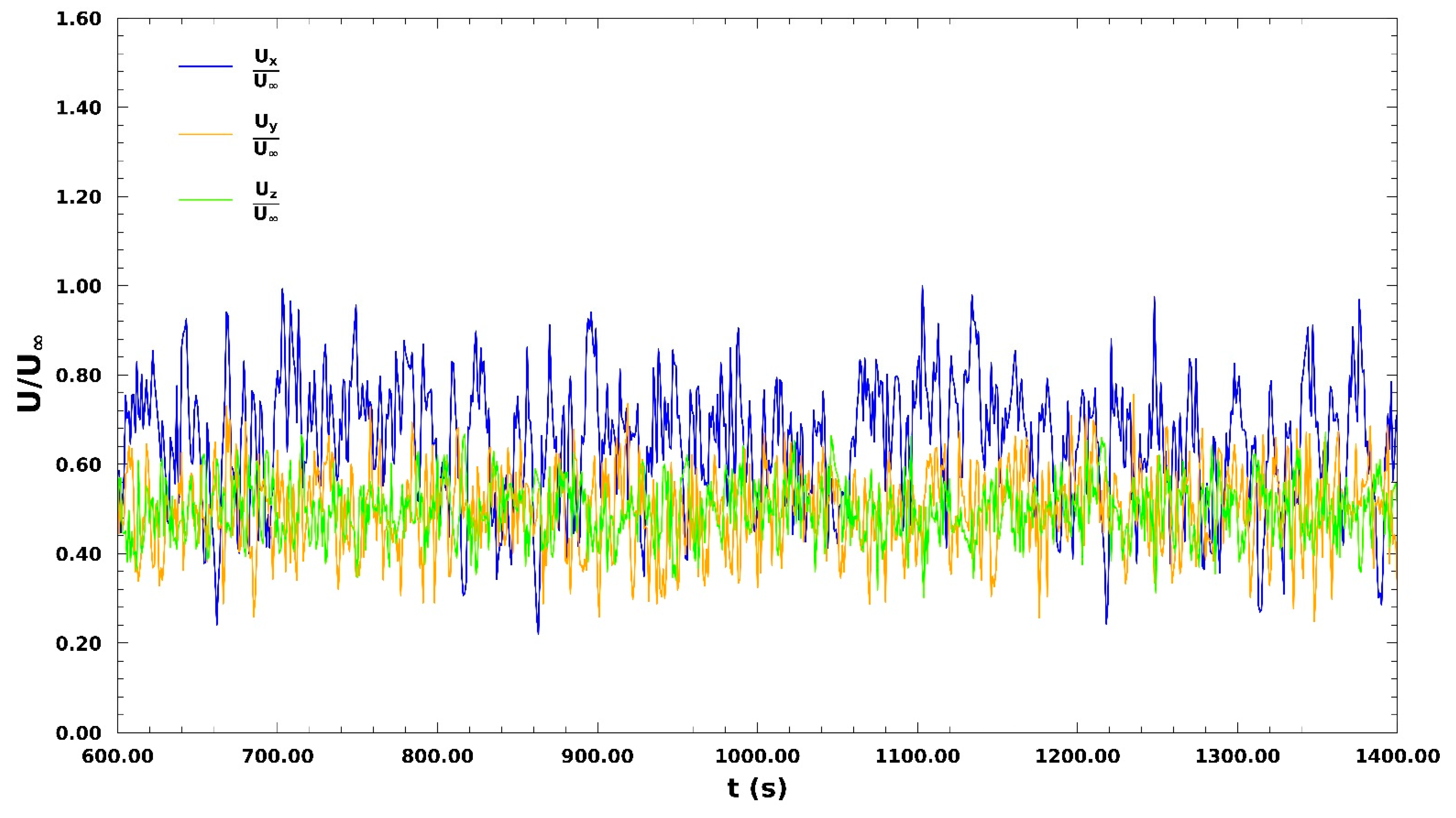
| Averaging Period (s) | Mean Value | Variance | Autocovariance |
|---|---|---|---|
| 600–800 | 1.0806 | 0.0473 | 0.3426 |
| 800–1000 | 1.0851 | 0.0538 | 0.3738 |
| 1000–1200 | 1.0879 | 0.0530 | 0.4316 |
| 1200–1400 | 1.0889 | 0.0524 | 0.4443 |
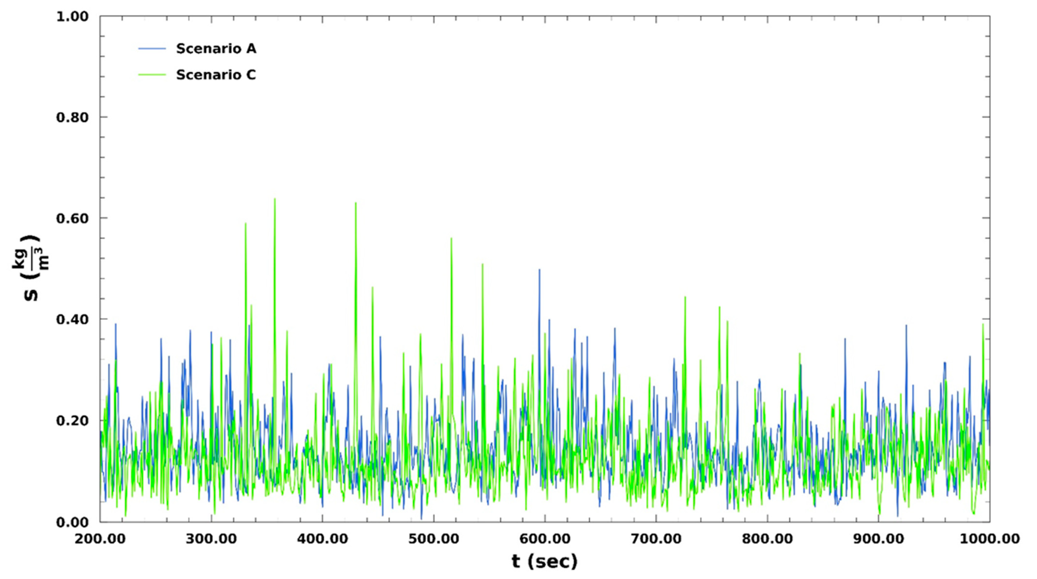
| Averaging Period (s) | Mean Value | Variance | Autocovariance |
|---|---|---|---|
| 200–400 | 0.2449 | 0.0186 | 0.9584 |
| 400–600 | 0.2445 | 0.0198 | 0.9532 |
| 600–800 | 0.2480 | 0.0193 | 0.9548 |
| 800–1000 | 0.2463 | 0.0195 | 0.9524 |
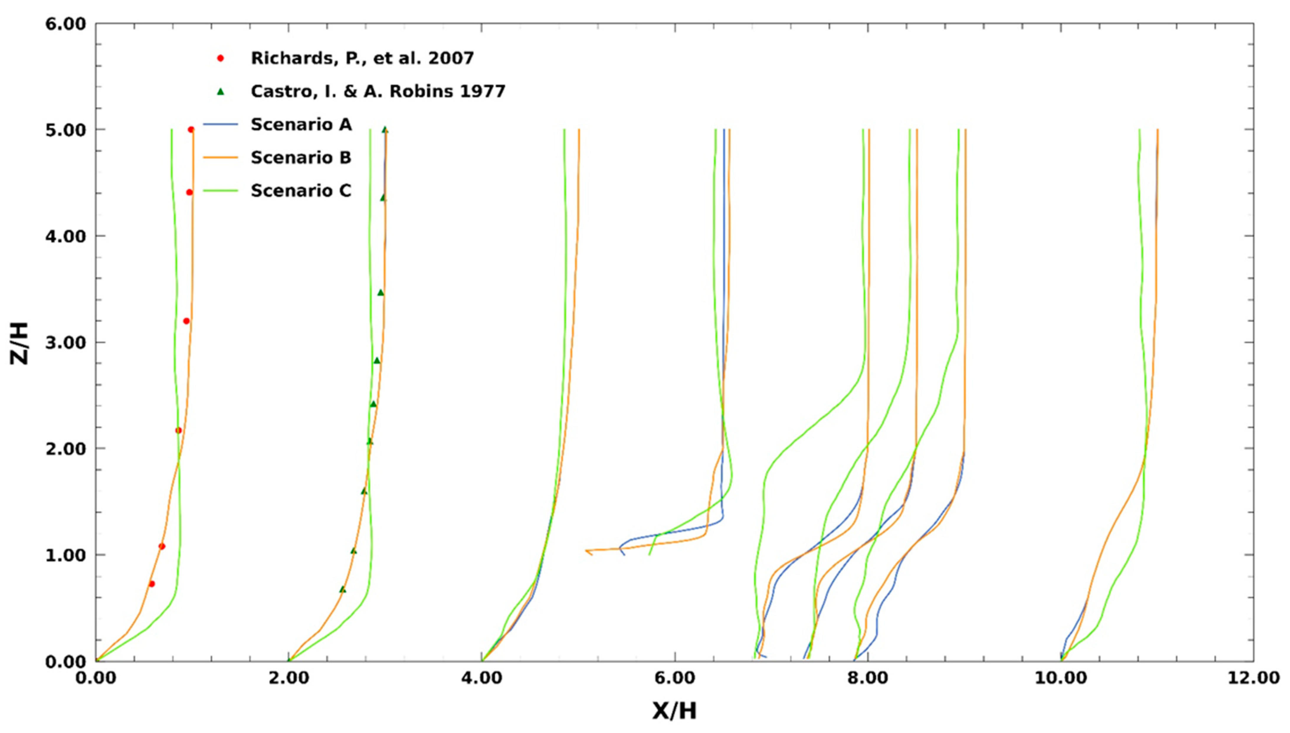
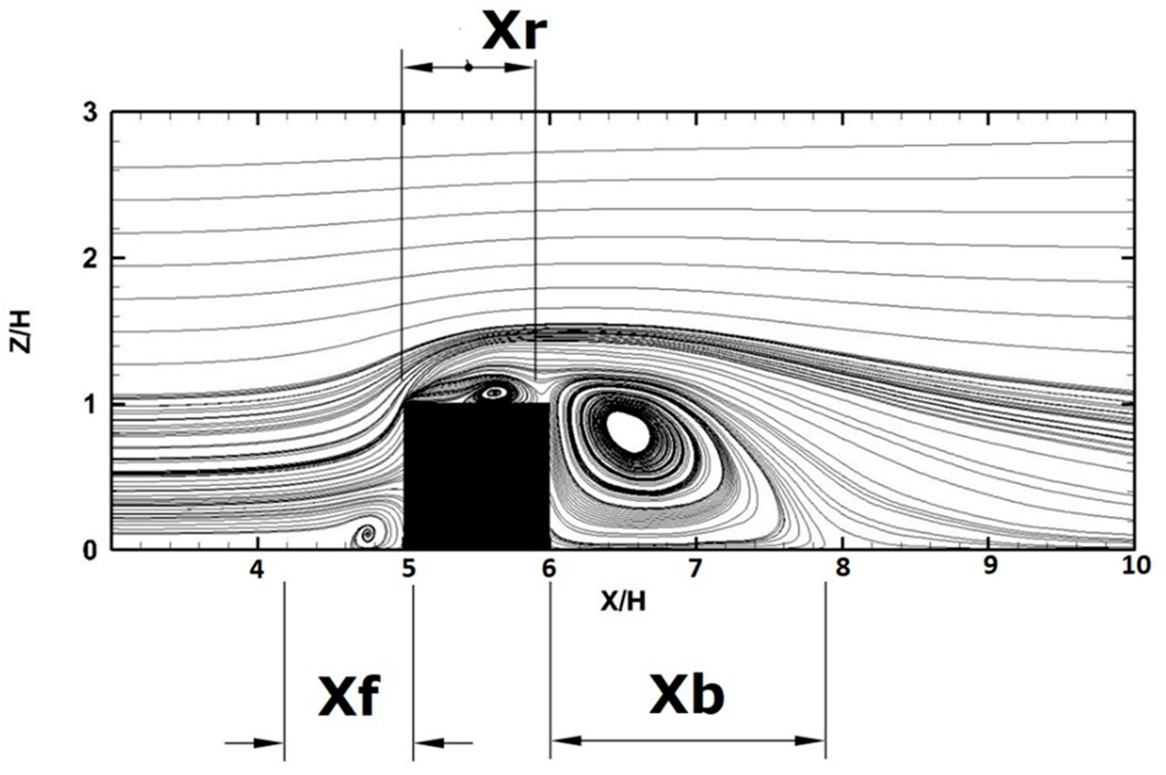
| Xf | Xb | Xr | |
|---|---|---|---|
| Martinuzzi and Tropea [61] | 1.04 H | 1.61 H | - |
| Rodi [62] | 0.651 H | 2.182 H | 0.432 H |
| Hoxey, Richards [63] | 0.75 H | 1.4 H | 0.57 H |
| Richards and Norris [64] | 0.9 H | 1.4 H | 0.9 H |
| Hu, Xuan [65] | - | 1.31 H | 0.94 H |
| Scenario A | 0.79 H | 1.56 H | 0.56 H |
| Scenario B | 0.56 H | 1.97 H | 0.64 H |
| Scenario C | 0.86 H | 2.15 H | 0.73 H |
Publisher’s Note: MDPI stays neutral with regard to jurisdictional claims in published maps and institutional affiliations. |
© 2022 by the authors. Licensee MDPI, Basel, Switzerland. This article is an open access article distributed under the terms and conditions of the Creative Commons Attribution (CC BY) license (https://creativecommons.org/licenses/by/4.0/).
Share and Cite
Pavlidis, C.L.; Palampigik, A.V.; Vasilopoulos, K.; Lekakis, I.C.; Sarris, I.E. Air Flow Study around Isolated Cubical Building in the City of Athens under Various Climate Conditions. Appl. Sci. 2022, 12, 3410. https://0-doi-org.brum.beds.ac.uk/10.3390/app12073410
Pavlidis CL, Palampigik AV, Vasilopoulos K, Lekakis IC, Sarris IE. Air Flow Study around Isolated Cubical Building in the City of Athens under Various Climate Conditions. Applied Sciences. 2022; 12(7):3410. https://0-doi-org.brum.beds.ac.uk/10.3390/app12073410
Chicago/Turabian StylePavlidis, Chariton L., Anargyros V. Palampigik, Konstantinos Vasilopoulos, Ioannis C. Lekakis, and Ioannis E. Sarris. 2022. "Air Flow Study around Isolated Cubical Building in the City of Athens under Various Climate Conditions" Applied Sciences 12, no. 7: 3410. https://0-doi-org.brum.beds.ac.uk/10.3390/app12073410