
Control of Flexible Robot by Harmonic Functions


Department of Mechanics, Biomechanics and Mechatronics, Faculty of Mechanical Engineering, CTU in Prague, Technicka 4, 166 00 Prague, Czech Republic
*
Author to whom correspondence should be addressed.
Appl. Sci. 2022, 12(7), 3604; https://0-doi-org.brum.beds.ac.uk/10.3390/app12073604
Submission received: 24 February 2022
/
Revised: 25 March 2022
/
Accepted: 30 March 2022
/
Published: 1 April 2022
(This article belongs to the Special Issue Sensors, Actuators and Methods in Active Noise and Vibration Control)
Abstract
:This work deals with the control of flexible structures as underactuated systems. The invariant control method performs the control of a flexible robot as a representative of an underactuated system with zero dynamics. The control input is separated into two parts. The arbitrary part of the control input is designed to control the directly actuated part of the dynamic system. The invariant part of the control is selected to steer the system zero dynamics in the desired way. The harmonic functions create the base for the invariant part of the control function. The residual vibration cancellation is the target of the presented invariant control strategy. The harmonic function frequencies are overtaken from the so-called natural motion, amplitudes are the results of the optimization process. The main target of this paper is to show the invariant control approach and its application to the system with flexible elements.
1. Introduction
This paper deals with the control of flexible structures as underactuated systems. The definition of underactuation should be based on the number of blocks in the Brunovsky canonical form [1]. The invariant control—its idea is presented in [2]—is used for flexible robot trajectory tracking with minimal residual oscillations. The desired trajectory is parametrized, exact input–output linearization is applied to the system coordinates (modal coordinates are excluded), and outputs are substituted by function of parametrization variables. This transformation assures that the robot endpoint follows the desired trajectory. Zero dynamics (system flexibility) oscillations are realized only in the perturbation of parametrization variables. The invariant control, based on the harmonic functions [3], is applied to the model of a flexible robotic arm, and its parameters are obtained using predictive optimization.
Many authors have already investigated the control of underactuated mechanical systems. Neurodynamic programming, as a main part of the control in [4], is used for the control of the ball and beam system. In [5], a method of adding the actuators to the underactuated joints and running the swing-up motion with optimization minimizing the action of the added actuators is used. Sliding mode control extended with fuzzy logic is introduced in [6] to control the motion of overhead crane. An approach with optimal control is used in [7]. The adaptive approach used for tracking control is presented in [8]. Partly stable controllers derived using the dynamic model of the manipulator create basis for the optimal switching sequence control in [9]. An energy-based approach used in the design of stabilizing controllers is presented in [10]. Friction forces are used in the energy control strategy in [11]. Authors in [12] introduce an averaging theory for controlling the systems with and without drift terms. In [13], the trajectory tracking controller is used for following the upward trajectory created from the downward simulation (similar to the natural motion in [14] and the natural oscillations in [15] of a parallel robot) and stabilizing trajectory. An active disturbance rejection control is designed in [16] for a pendubot system. The walking-like trajectory tracking of an acrobot is continuously developed in [17]. A 3D bipedal gait walking robot is presented in [18], and the development of humanoid motion design is investigated in [19]. The robust sliding mode control is developed for stabilizing and trajectory tracking of a ballbot system in [20], and the wheel-legged biped robot motion is stabilized using active arm manipulator in [21]. The dynamic balancing of quadruped robot with optimal controller is presented in [22], and a different quadruped robot design is presented in [23]. Ref. [24] presents linear quadratic regulator applied to control vertical take-off and landing (VTOL) multi-rotor vehicle with passive rotor tilting mechanism. A control based on a function approximation technique using the variation of an approximated square system is presented in [25,26]. The cyclic control using sinusoids for nonholonomic systems is presented in [27] (stabilization), and motion planning is presented in [28]. The control of a wheeled, inverted pendulum is transferred into dynamic trajectory planning with a boundary value problem in [29]. State feedback fuzzy system controller, based on , is investigated in [30]. The underactuated mechanisms in the gravity field can be controlled in their equilibrium positions (see [31]), but there are always singularity points between these equilibrium states. To move the mechanism through this region (see [32]) is a challenging task, and the work in [14] shows one possible way to overcome it.
The investigation of system flexibility as a system underactuation is usually investigated with linearized stiffness; the authors of [33] deal with dynamic coupling of such underactuated manipulators. Modelling flexibility in underactuated systems by a rotational spring is presented in [34], and a similar flexibility model is investigated in [35], where the spring stiffness is varied, and a point stabilization control is developed. A model with linear springs is investigated in [36], where input–output linearization is performed along with a PID controller. Sliding mode control is used to control the flexible robotic arm in [37]. The current work aims to introduce the invariant control strategy to the structures with compliancy (chain of flexible robotic arms). The nonlinear system with flexible modes is obtained using the procedure presented in [38].
An invariant control is presented in [2]. The application of such control to the underactuated system (double pendulum, double pendulum on a cart) is shown in [14,39]. The current work does not include the flexible structures and does not deal with trajectory tracking. This paper aims to introduce the control strategy to the structures with compliancy—in our case, the flexible robotic arm. Another contribution of the paper is in its presentation of a control strategy which forces the undesired movements of the system into the desired system endpoint trajectory.
The paper is organized as follows. The exact input–output linearization is presented in Section 2 for underactuated systems. Next, the coordinates are separated into actuated and unactuated. Then, consecutive output parameterization is introduced. Section 2.1 introduces invariant control with harmonic functions and the natural motion used for the Eigen frequency evaluation. Section 3 introduces the presented method to flexible robotic arm: modelling and parameterization with input–output linearization is applied to the flexible robot. Next, the particular control application to the flexible robotic arm and simulation results are presented. Section 4 concludes the work.
2. Materials and Methods
The control of underactuated, flexible structure using invariant control is presented.
2.1. Exact Input–Output Linearization with Parametrization
Let us consider a nonlinear dynamic system (Eigen equations of motion):
where the matrix is an inertia matrix; are coordinates describing the system; and their time derivatives; is a matrix containing forces dependent on velocities and external forces besides control inputs; is the control input distribution matrix; the vector contains the control inputs.
The state vector could be rewritten without loss of generality in the following way:
where has the same dimension as the rank of matrix . Remaining z coordinates in vector represent not directly actuated states (zero dynamics). This coordinate selection is generally not unique. The system (1) could be rewritten as follows:
where the matrix is the largest regular sub-matrix of the matrix with the rank a (the actuator redundancy is not covered, so ). The number of coordinates is . The matrix dimensions in (3) and (4) are dependent on the lower indexes, and matrix has dimensions . Let us consider the vector of system outputs of the same dimension as the vector . There is a relation between system outputs and system coordinates:
with a vector representing the dependence of the output on the system coordinates and . There exist the inverse relation , such that the coordinates and its second time derivative can be uniquely determined:
where , and are matrices resulting the time derivatives. The outputs are often parametrized, especially in robotics applications. The parametrized trajectory is defined:
with the following output acceleration:
where vector is output parametrization and , are time derivative resulting matrices with p equalling the number of parameters. The inputs are expressed from (3) and substituted into (4), and then the second time derivative of , much like from (7) and (9), are substituted, and the final set of equations is obtained:
where
2.2. Invariant Control
In this section, the control variable is assembled. There is a dynamic system to be controlled (derived from the previous section):
The input variable directly influences parameters of . However, how can the zero dynamics coordinates be controlled? The proposed way is to split the input variable into arbitrary part , which controls the parameters , and invariant part , which controls coordinates , with specific influence on parameters .
The arbitrary part is assembled to reach the final configuration at time, T. The invariant part must satisfy invariancy conditions (16). Hence it modifies parameters and their time derivatives only inside the interval . The invariancy conditions are the following:
If the input variable (15) is substituted into the (13), and the system of equations is integrated from to , then the following is obtained:
From (17), it is obvious that parameters and their time derivatives at the end (final) time depend only on the arbitrary part of the control (15). The arbitrary part could be arbitrarily chosen, just to fulfil the end position and velocities of the parameters . After the selection of the arbitrary part of the control, it is a time-dependent part, and (14) changes into (18).
The invariant part of the control must fulfil the conditions of (16), and the control coordinates from (18) must reach the desired states at the end time, T. The suitable functions are the following harmonic functions:
The parameters , of harmonic functions (19) are obtained from the optimization process, and the frequencies, , are based on the so-called natural motion.
2.3. Natural Motion
According to [14], natural motion is derived from the vicinity of an unstable equilibrium to the vicinity of a stable equilibrium. The motion takes place in the gravity field with dissipative members instead of actuators. It is helpful to rearrange the formulation for the flexible systems. For obtaining the natural motion, it is used the simulation with zero invariant part , controlled only with the arbitrary part of the control . The system is moved from the initial position to the end position, where the system stays, and residual (zero dynamics) vibrations are exerted.
All system states are recorded during the motion, and the frequencies, , are obtained from the frequency analysis of the recorded behaviour.
3. Results
The present section introduces the presented procedure with invariant control to the flexible robotic structure.
3.1. Model of Flexible Robot
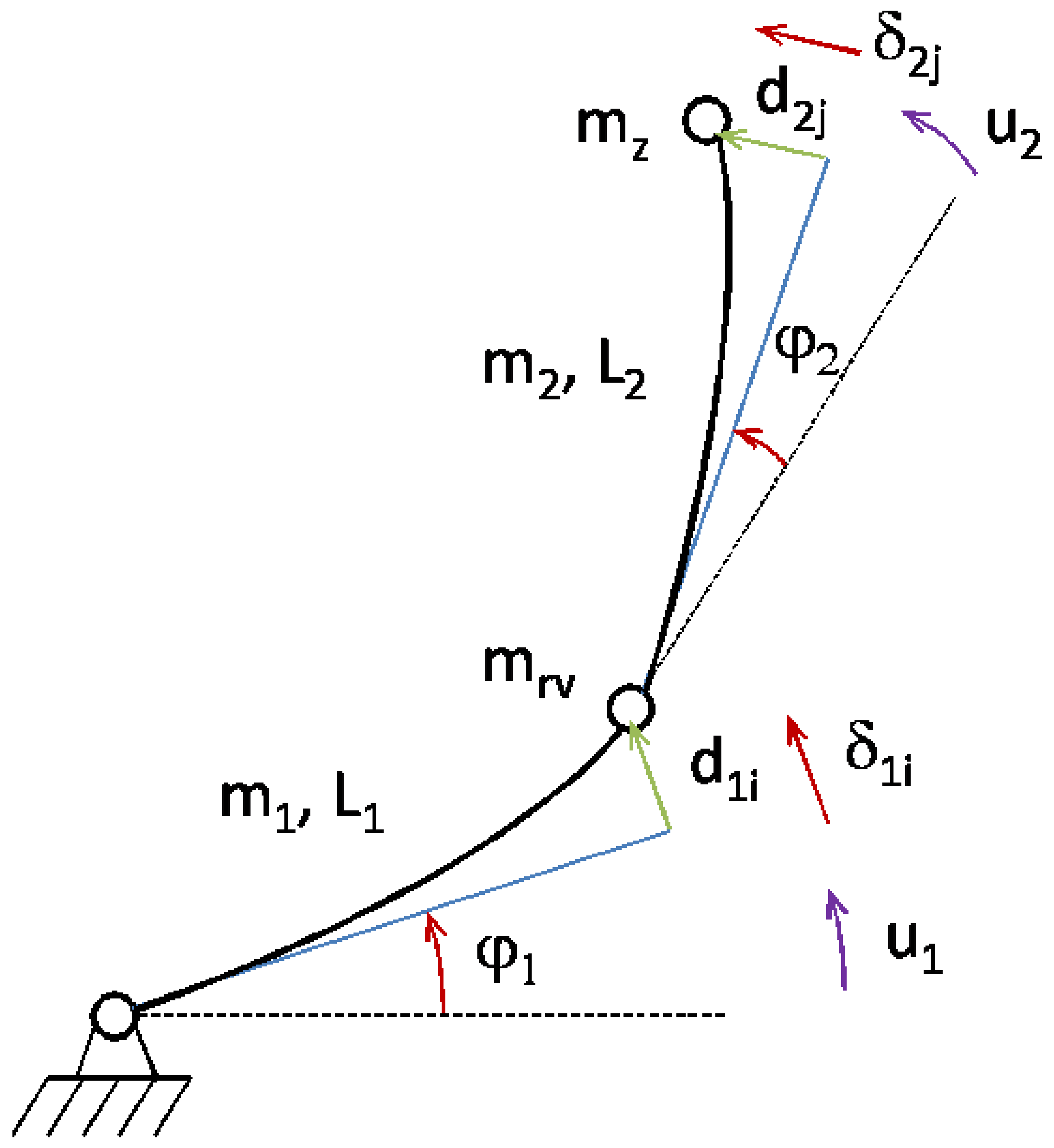
A flexible robot is modelled as a double pendulum with flexible arms. It consists of two flexible beams, interconnected by a revolute joint, and coupled to the base frame with the second revolute joint. Every beam has flexibility modelled by three modes. There are actuators in each revolute joint. The model covers the mass of the actuator, and the endpoint is loaded by extra mass. The system is situated in the gravity field, see Figure 1.
Eigen equations of motion of the flexible double pendulum are obtained using the procedure derived in [38]. The implementation is presented in [40]. The Eigen equations of motion are in the following form:
where
Furthermore, matrix is an inertia matrix, vector covers velocity-dependent forces, gravity forces, and damping forces, and , are actuator moments. Beam k endpoint position is determined by angular rotation and beam deflection . Beam deflection is obtained according to the following equation:
where are dimensionless modal coordinates and are coefficients of modal parameters beam deflection at particular point. The angular deflection of the first beam endpoint is needed for the determination of the second beam position. This endpoint angular deflection is indicated as , and generally
where are coefficients of modal parameters, beam angular deflection at particular point. Angle is the relative angle between the un-deformed shape of the first beam and its endpoint angular deflection (or endpoint tangent to deformed beam shape).
3.2. Input–Output Linearization with Output Parametrization
It is necessary to split the state vector into and according to (2). The claim on the regularity of submatrix derived from matrix in (20) directly implies the splitting of vector :
The flexible double pendulum endpoint coordinates and are system outputs , and it corresponds with the length of vector . Input–output linearization can be accomplished. Outputs are obtained using the following relations:
The coordinates in the vector are now changed to the end effector (double pendulum endpoint) coordinates. Equation (24) is used to obtain coordinates and its time derivatives according to (6) and (7) to be substituted into (20). Following one dimensional parametrization (typically endpoint trajectory, see (25)) ensures the endpoint position and leaves free movement along this parameter. Then, the zero dynamics control actions use this free parameter for realizing its unwanted movements.
The system inputs are obtained from (12), but the following procedure could also be used. Outputs functions (24) and their parametrization (25) are the second-time derivate:
In (26), the coordinates acceleration are substituted from (20), and outputs acceleration , are replaced from (27). The control inputs are obtained from the resulting alternative expression:
The right-hand side of (28) also depends on the state vector and its time derivative . Therefore, inputs could also be evaluated according to (12) in the form with only p and coordinates.
The advantage of such a strategy is that flexible robot endpoint never leaves the prescribed trajectory, and zero dynamics () control actions are realized only along the parameter, p.
3.3. Control of Flexible Robot
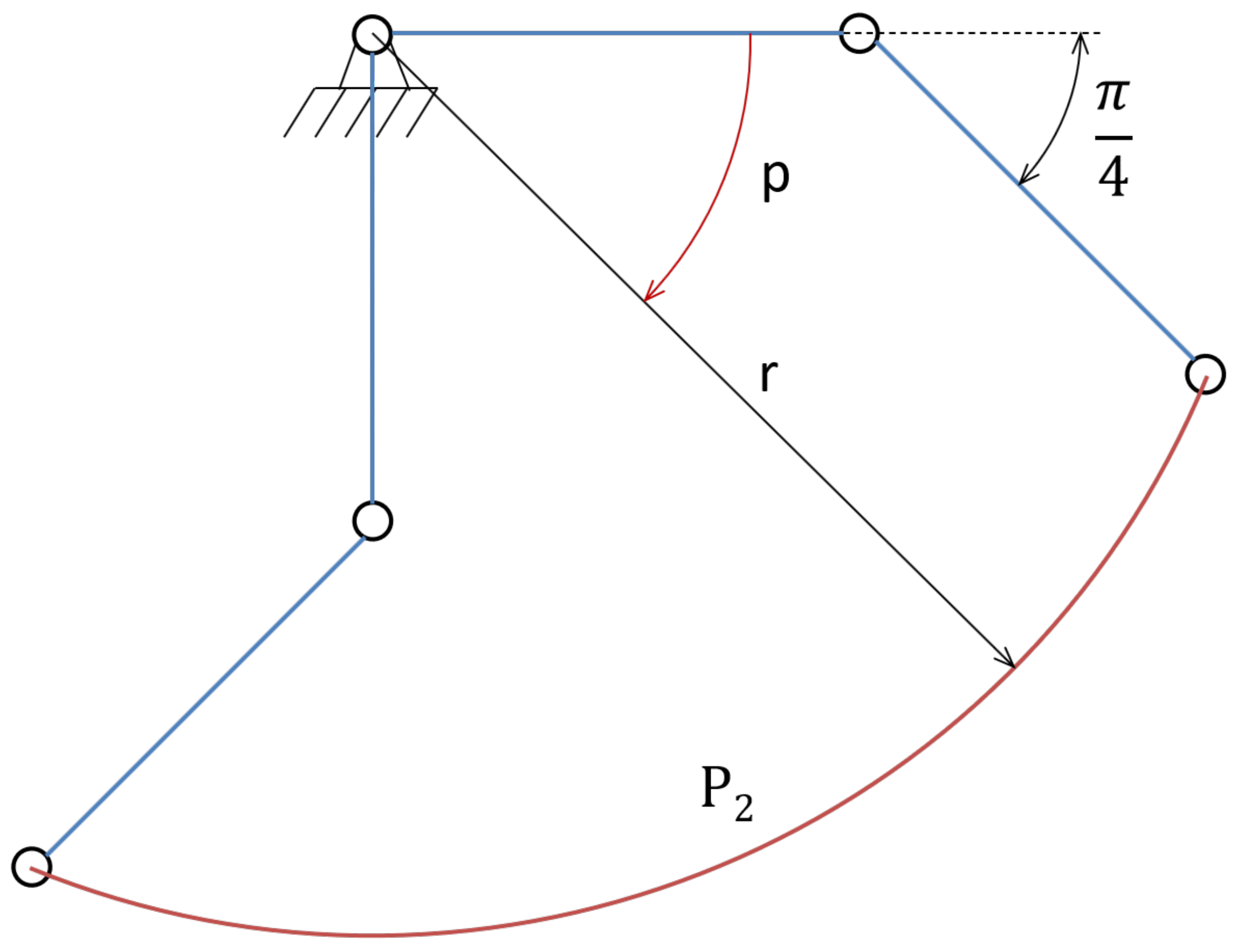
The task is to move the flexible robot endpoint along the circle arc, see Figure 2. The circle centre is in the joint between the base frame and the first arm. The radius is r in (29), and the circle parameter p is angular position measured from the robot’s initial position.
At first, the arbitrary part of the control () is prepared. According to (13), the input is the second time derivative of parameter p. Design of arbitrary part of the control is based on the parameter p behaviour. The initial position and end position have velocities and accelerations selected to be zero. Such conditions satisfy a fifth-order polynomic in function p, see Figure 3. Movement duration is one of the free parameters, but it will be determined by the desired speed of the robot endpoint.
3.3.1. Natural Motion Frequencies
Natural motion is performed only with arbitrary part of the control with the duration of 1 s. When the robot reaches the end position, residual vibrations are measured, see Figure 4, left. It is evident that all system coordinates vibrate at just one natural frequency ( Hz), and this is verified by the frequency analysis in Figure 4, right. For the different simulation times, the resulting natural motion frequency is the same.
3.3.2. Invariant Control Parameters
The invariant part of the control is constructed according to (19). The optimization process is performed to obtain the number of intervals , natural frequency multiplication factors for obtaining particular , phase , and corresponding amplitudes . The phase is same for all frequencies .
The objective function aims to fulfil the prescribed trajectory endpoint position and velocity. Physical coordinates and modal coordinates at end time should be ideally equal to the trajectory endpoint static position and their time derivatives (velocities) should be zero, see (30).
The optimization process minimizes the objective function in (30), where are variable weights, is prescribed movement end time, and are prescribed movement endpoint coordinates.
The extensive optimization brings three frequency multiplication factors , and , with resulting frequency , the 16 intervals of , and amplitudes shown in Table 1.
3.4. Simulation
The applied control forces the robot endpoint to move along the desired trajectory. The difference between the control methods (computed torques method and invariant control) is in the behaviour of the zero dynamics movements from the end time of motion. The computed torque method cannot effectively cancel out zero dynamics oscillations after reaching the final position. The invariant control implies slightly different claim on the system torques and than the computed torque method, but after reaching the final time, the system is still. The influence of invariant control to the desired parameter p behaviour is on Figure 5. The amplitude of the parameter, p, invariant control modification is significantly low in comparison with the desired motion change.
Figure 6 and Figure 7 show the behaviour of and input torques, respectively. The plot of Figure 6 shows the first input torque needed for satisfying the desired motion. There are two curves, one is dedicated for the computed torques method, and the second one corresponds to the torque claim of the invariant control. In the cut is the detailed behaviour after the prescribed motion final time. Invariant control modifies input torque so that there is no residual vibration of zero dynamics, contrary to the computed torque method. The second part of Figure 6 graph shows the difference between computed torques and invariant control behaviour. The red curve represents modification of computed torques , claimed due to the invariant part of the control, and the blue line shows the residual (zero dynamics) vibrations of the system with control using the computed torques method. The corresponding behaviour of input torque is shown on Figure 7.
The advantage of invariant control is that the system moves from one equilibrium to another equilibrium position. The input torque is modified within of the reference torque (computed torque method serves as the reference). The movement within parameter, p, is the only disadvantage of the invariant control, but it is of small amplitude, as shown on Figure 5 (bottom).
4. Conclusions
The control of a flexible robot as a representative of underactuated system with zero dynamics is performed using invariant control method. The basis of invariant control are harmonic functions, which are used for feedforward control of particular flexible system. The harmonic functions provide smooth motion as is needed for vibration cancellation when reaching the desired position. Presented here is an invariant control of flexible underactuated structure in connection with observing the desired trajectory.
The control strategy uses motion frequencies inspired by so-called natural motion. The residual oscillations provide the natural motion frequency, which is used to cancel out unwanted vibrations. The control input is separated into two parts. The arbitrary part of the control input () is designed to control the directly actuated part of the dynamic system. The invariant part of the control () is selected to steer the system zero dynamics in the desired way. The invariant part of the control fulfils the invariant conditions with respect to overall control input behaviour. The amplitudes of chosen periodic functions are obtained by optimization process with the final position in objective function. The achieved accuracy depends on the optimization process inputs, the trajectory length, and the number of used frequencies. The control parameters are predicted using the optimization process and resulting tracking accuracy is the same for the same trajectory.
The main aim of this work was to present the functionality of an invariant control approach to a system with flexible elements. Further research will focus on the extension of the invariant control by feedback to avoid the optimization process. The proposed concept will be enhanced by the model predictive, wave-based or sliding mode control to secure missing feedback. To fulfil the invariance conditions (16) the control strategy will be formulated in discrete form.. The presented control can be practically applied in serial robotics, i.e., robotic manipulators or machine tools.
Author Contributions
Conceptualization, M.V. and M.N.; software experiment, Z.N.; writing—original draft preparation, Z.N. and M.N. All authors have read and agreed to the published version of the manuscript.
Funding
This work was supported by the European Regional Development Fund under the project Robotics for Industry 4.0 (reg. no. CZ.02.1.01/0.0/0.0/15 003/0000470).
Conflicts of Interest
The authors declare no conflict of interest.
References
- Valášek, M. Design and control of under-actuated and over-actuated mechanical systems—Challenges of mechanics and mechatronics. Suppl. Veh. Syst. Dyn. 2002, 40, 37–50. [Google Scholar]
- Valášek, M. Control of elastic industrial robots by nonlinear dynamic compensation. Acta Polytech. 1993, 33, 15–30. [Google Scholar]
- Neusser, Z.; Valášek, M. Control of the underactuated mechanical systems by harmonics. In Proceedings of the ECCOMAS Thematic Conference on Multibody Dynamics, Zagreb, Croatia, 1–4 July 2013; pp. 329–339. [Google Scholar]
- Burghardt, A.; Szuster, M. Neuro-Dynamic Programming in Control of the Ball and Beam System. In Solid State Phenomena; Mechatronic Systems, Mechanics and Materials II; Trans Tech Publications, Ltd.: Freienbach, Switzerland, 2014; Volume 210, pp. 206–214. [Google Scholar] [CrossRef]
- Rubí, J.; Rubio, A.; Avello, A. Swing-up control problem for a self-erecting double inverted pendulum. IEE Proc. Control. Theory Appl. 2002, 149, 169–175. [Google Scholar] [CrossRef]
- Liu, D.; Yi, J.; Zhao, D.; Wang, W. Adaptive sliding mode fuzzy control for a two-dimensional overhead crane. Mechatronics 2005, 15, 505–522. [Google Scholar] [CrossRef]
- Liu, Z.; Yang, T.; Sun, N.; Fang, Y. An Antiswing Trajectory Planning Method with State Constraints for 4-DOF Tower Cranes: Design and Experiments. IEEE Access 2019, 7, 62142–62151. [Google Scholar] [CrossRef]
- Kim, J.; Kiss, B.; Kim, D.; Lee, D. Tracking Control of Overhead Crane Using Output Feedback with Adaptive Unscented Kalman Filter and Condition-Based Selective Scaling. IEEE Access 2021, 9, 108628–108639. [Google Scholar] [CrossRef]
- Udawatta, L.; Watanabe, K.; Izumi, K.; Kiguchi, K. Control of underactuated robot manipulators using switching computed torque method: GA based approach. Soft Comput. 2003, 8, 51–60. [Google Scholar] [CrossRef]
- Fantoni, I.; Lozano, R. Non-linear Control for Underactuated Mechanical Systems; Springer: London, UK, 2002. [Google Scholar] [CrossRef]
- Mahindrakar, A.D.; Rao, S.; Banavar, R. Point-to-point control of a 2R planar horizontal underactuated manipulator. Mech. Mach. Theory 2006, 41, 838–844. [Google Scholar] [CrossRef] [Green Version]
- Vela, P.A. Averaging and Control of Nonlinear Systems. Ph.D. Thesis, California Institute of Technology, Pasadena, CA, USA, 2003. [Google Scholar] [CrossRef]
- Zhang, A.; She, J.; Lai, X.; Wu, M. Motion planning and tracking control for an acrobot based on a rewinding approach. Automatica 2013, 49, 278–284. [Google Scholar] [CrossRef]
- Neusser, Z.; Valášek, M. Control of the underactuated mechanical systems using natural motion. Kybernetika 2012, 48, 223–241. [Google Scholar]
- Idà, E.; Briot, S.; Carricato, M. Natural Oscillations of Underactuated Cable-Driven Parallel Robots. IEEE Access 2021, 9, 71660–71672. [Google Scholar] [CrossRef]
- Ramírez-Neria, M.; Sira-Ramírez, H.; Garrido-Moctezuma, R.; Luviano-Juárez, A.; Gao, Z. Active Disturbance Rejection Control for Reference Trajectory Tracking Tasks in the Pendubot System. IEEE Access 2021, 9, 102663–102670. [Google Scholar] [CrossRef]
- Anderle, M.; Čelikovský, S. Feedback design for the Acrobot walking-like trajectory tracking and computational test of its exponential stability. In Proceedings of the 2011 IEEE International Symposium on Computer-Aided Control System Design (CACSD), Denver, CO, USA, 28–30 September 2011; pp. 1026–1031. [Google Scholar] [CrossRef]
- Da, X.; Harib, O.; Hartley, R.; Griffin, B.; Grizzle, J.W. From 2D Design of Underactuated Bipedal Gaits to 3D Implementation: Walking with Speed Tracking. IEEE Access 2016, 4, 3469–3478. [Google Scholar] [CrossRef]
- Zielinska, T.; Rivera Coba, G.R.; Ge, W. Variable Inverted Pendulum Applied to Humanoid Motion Design. Robotica 2021, 39, 1368–1389. [Google Scholar] [CrossRef]
- Lee, S.M.; Park, B.S. Robust Control for Trajectory Tracking and Balancing of a Ballbot. IEEE Access 2020, 8, 159324–159330. [Google Scholar] [CrossRef]
- Raza, F.; Zhu, W.; Hayashibe, M. Balance Stability Augmentation for Wheel-Legged Biped Robot Through Arm Acceleration Control. IEEE Access 2021, 9, 54022–54031. [Google Scholar] [CrossRef]
- Chignoli, M.; Wensing, P.M. Variational-Based Optimal Control of Underactuated Balancing for Dynamic Quadrupeds. IEEE Access 2020, 8, 49785–49797. [Google Scholar] [CrossRef]
- Kanner, O.Y.; Rojas, N.; Odhner, L.U.; Dollar, A.M. Adaptive Legged Robots Through Exactly Constrained and Non-Redundant Design. IEEE Access 2017, 5, 11131–11141. [Google Scholar] [CrossRef]
- Iriarte, I.; Iglesias, I.; Lasa, J.; Calvo-Soraluze, H.; Sierra, B. Enhancing VTOL Multirotor Performance with a Passive Rotor Tilting Mechanism. IEEE Access 2021, 9, 64368–64380. [Google Scholar] [CrossRef]
- Bai, Y.; Svinin, M. Motion Planning and Control for a Class of Partially Differentially Flat Systems. In Proceedings of the 2019 12th International Conference on Developments in eSystems Engineering (DeSE), Kazan, Russia, 7–10 October 2019; pp. 855–860. [Google Scholar] [CrossRef]
- Bai, Y.; Svinin, M.; Magid, E.; Wang, Y. On Motion Planning and Control for Partially Differentially Flat Systems. Robotica 2020, I, 718–734. [Google Scholar] [CrossRef]
- Teel, A.R.; Murray, R.M.; Walsh, G. Nonholonomic control systems: From steering to stabilization with sinusoids. In Proceedings of the 31st IEEE Conference on Decision and Control, Tucson, AZ, USA, 16–18 December 1992; Volume 2, pp. 1603–1609. [Google Scholar] [CrossRef]
- Murray, R.M.; Sastry, S.S. Nonholonomic motion planning: Steering using sinusoids. IEEE Trans. Autom. Control. 1993, 38, 700–716. [Google Scholar] [CrossRef] [Green Version]
- Kim, S.; Kwon, S. Robust transition control of underactuated two-wheeled self-balancing vehicle with semi-online dynamic trajectory planning. Mechatronics 2020, 68, 102366. [Google Scholar] [CrossRef]
- Elkinany, B.; Alfidi, M.; Chaibi, R.; Chalh, Z. T-S Fuzzy System Controller for Stabilizing the Double Inverted Pendulum. Adv. Fuzzy Syst. 2020, 2020, 8835511. [Google Scholar] [CrossRef]
- Olfati-Saber, R. Nonlinear Control of Underactuated Mechanical Systems with Application to Robotics and Aerospace Vehicles. Ph.D. Thesis, Massachusetts Institute of Technology, Cambridge, CA, USA, 2001. [Google Scholar]
- Aneke, N. Control of Underactuated Mechanical Systems. Ph.D. Thesis, Eindhoven University of Technology, Eindhoven, The Netherlands, 2003. [Google Scholar] [CrossRef]
- Zhao, T.S.; Dai, J.S. Dynamics and Coupling Actuation of Elastic Underactuated Manipulators. J. Robot. Syst. 2003, 20, 135–146. [Google Scholar] [CrossRef]
- He, G.P.; Geng, Z.Y. The nonholonomic redundancy of second-order nonholonomic mechanical systems. Robot. Auton. Syst. 2008, 56, 583–591. [Google Scholar] [CrossRef]
- Xin, X.; Liu, Y. A Set-Point Control for a Two-link Underactuated Robot with a Flexible Elbow Joint. J. Dyn. Syst. Meas. Control. 2013, 135, 051016. [Google Scholar] [CrossRef]
- Chen, W.; Zhao, L.; Zhao, X.; Yu, Y. Control of the Underactuated Flexible Manipulator in the Operational Space. In Proceedings of the 2009 International Conference on Intelligent Human–Machine Systems and Cybernetics, Hangzhou, China, 26–27 August 2009; Volume 2, pp. 470–473. [Google Scholar] [CrossRef]
- Rodriguez-Cianca, D.; Rodriguez-Guerrero, C.; Verstraten, T.; Jimenez-Fabian, R.; Vanderborght, B.; Lefeber, D. A Flexible shaft-driven Remote and Torsionally Compliant Actuator (RTCA) for wearable robots. Mechatronics 2019, 59, 178–188. [Google Scholar] [CrossRef]
- Vampola, T.; Valášek, M. Composite rigid body formalism for flexible multibody systems. Multibody Syst. Dyn. 2007, 18, 413–433. [Google Scholar] [CrossRef]
- Neusser, Z.; Valášek, M. Control of the double inverted pendulum on a cart using the natural motion. Acta Polytech. 2013, 53, 883–889. [Google Scholar] [CrossRef]
- Mráz, L. Symbolické Generování Pohybových Rovnic pro Soustavy Poddajných Těles. Master’s Thesis, Czech Technical University in Prague, Prague, Czech Republic, 2010. (In Czech). [Google Scholar]
Figure 1.
Model of robot with two flexible arms.

Figure 2.
Flexible robot endpoint trajectory.

Figure 3.
Behaviour of parameter p (endpoint angle) and its time derivatives and .

Figure 4.
Natural motion: residual vibrations. (a) Coordinates of time behaviour; (b) power spectra density with significant Eigen frequency of Hz.
Figure 4.
Natural motion: residual vibrations. (a) Coordinates of time behaviour; (b) power spectra density with significant Eigen frequency of Hz.

Figure 5.
Trajectory parameter p behaviour (upper part) for the time interval and its invariant control modification (bottom part).
Figure 5.
Trajectory parameter p behaviour (upper part) for the time interval and its invariant control modification (bottom part).

Figure 6.
System input torque behaviour for two types of control—computed torques and invariant control and their difference.
Figure 6.
System input torque behaviour for two types of control—computed torques and invariant control and their difference.

Figure 7.
System input torque behaviour for two types of control—computed torques and invariant control and their difference.
Figure 7.
System input torque behaviour for two types of control—computed torques and invariant control and their difference.


Table 1.
Amplitudes.
| 1 | −0.0256 | 0.0504 | 0.0050 |
| 2 | −0.0251 | −0.0502 | 0.0051 |
| 3 | 0.0253 | 0.0500 | 0.0050 |
| 4 | 0.0255 | −0.0506 | −0.0050 |
| 5 | −0.0253 | 0.0523 | −0.0050 |
| 6 | −0.0264 | −0.0494 | −0.0050 |
| 7 | 0.0251 | 0.0514 | 0.0051 |
| 8 | 0.0263 | −0.0407 | 0.0051 |
| 9 | −0.0251 | 0.0050 | |
| 10 | −0.0252 | −0.0051 | |
| 11 | 0.0253 | −0.0051 | |
| 12 | 0.0251 | −0.0050 | |
| 13 | −0.0253 | 0.0050 | |
| 14 | −0.0252 | 0.0050 | |
| 15 | 0.0244 | 0.0050 | |
| 16 | 0.0225 | −0.0050 | |
| 17 | −0.0050 | ||
| 18 | −0.0051 | ||
| 19 | 0.0051 | ||
| 20 | 0.0051 | ||
| 21 | 0.0052 | ||
| 22 | −0.0050 | ||
| 23 | −0.0050 | ||
| 24 | −0.0051 |
Publisher’s Note: MDPI stays neutral with regard to jurisdictional claims in published maps and institutional affiliations. |
© 2022 by the authors. Licensee MDPI, Basel, Switzerland. This article is an open access article distributed under the terms and conditions of the Creative Commons Attribution (CC BY) license (https://creativecommons.org/licenses/by/4.0/).
Share and Cite
MDPI and ACS Style
Neusser, Z.; Nečas, M.; Valášek, M. Control of Flexible Robot by Harmonic Functions. Appl. Sci. 2022, 12, 3604. https://0-doi-org.brum.beds.ac.uk/10.3390/app12073604
AMA Style
Neusser Z, Nečas M, Valášek M. Control of Flexible Robot by Harmonic Functions. Applied Sciences. 2022; 12(7):3604. https://0-doi-org.brum.beds.ac.uk/10.3390/app12073604
Chicago/Turabian StyleNeusser, Zdeněk, Martin Nečas, and Michael Valášek. 2022. "Control of Flexible Robot by Harmonic Functions" Applied Sciences 12, no. 7: 3604. https://0-doi-org.brum.beds.ac.uk/10.3390/app12073604
Note that from the first issue of 2016, this journal uses article numbers instead of page numbers. See further details here.