
Efficient Computer-Generated Holography Based on Mixed Linear Convolutional Neural Networks


College of Science, China University of Petroleum (East China), Qingdao 266580, China
*
Author to whom correspondence should be addressed.
Appl. Sci. 2022, 12(9), 4177; https://0-doi-org.brum.beds.ac.uk/10.3390/app12094177
Submission received: 28 March 2022
/
Revised: 17 April 2022
/
Accepted: 18 April 2022
/
Published: 21 April 2022
(This article belongs to the Special Issue Holography, 3D Imaging and 3D Display Volume II)
Abstract
:Imaging based on computer-generated holography using traditional methods has the problems of poor quality and long calculation cycles. However, recently, the development of deep learning has provided new ideas for this problem. Here, an efficient computer-generated holography (ECGH) method is proposed for computational holographic imaging. This method can be used for computational holographic imaging based on mixed linear convolutional neural networks (MLCNN). By introducing fully connected layers in the network, the suggested design is more powerful and efficient at information mining and information exchange. Using the ECGH, the pure phase image required can be obtained after calculating the custom light field. Compared with traditional computed holography based on deep learning, the method used here can reduce the number of network parameters needed for network training by about two-thirds while obtaining a high-quality image in the reconstruction, and the network structure has the potential to solve various image-reconstruction problems.
1. Introduction
Digital holography [1,2,3] can be used in the recording and playback of object waves based on interference and diffraction. The recording process, however, is always affected by many factors since the optical interference is vulnerable to its environment. Computer-generated holography (CGH) is a light field modulation technique that obtains a custom light field distribution by encoding the intensity or phase of the coherent light wave-fronts. Especially for phase-only computational holography, the image displayed can be realized without the disturbance of a zero term and a twin image. The development of spatial light modulator (SLM) technology or a meta-material membrane provides a physical carrier for the realization of this technology. The intensity and phase modulation of spatial light can be realized by loading a specific gray scale image on the intensity or phase modulation SLM, respectively. CGH is also a light field modulation method that has been garnering much interest and has been applied to holographic light traps [4,5], neural light stimulation [6,7], 3D display [8,9,10,11,12], planar solar concentrators [13,14], and near-eye AR displays [15,16].
The goal of CGH is to obtain optimal wave modulation by inversely solving a custom light field. This problem is always a nonlinear, ill-posed non-convex inverse problem, and the solved wave modulation must be a free-space solution of the wave propagation equation. At the same time, the image quality is limited by the modulation accuracy of the SLM. It is usually difficult to represent the target light field. In practice, the solution of computational holograms is always an approximation, and numerical methods are required to determine a feasible hologram to obtain the best encoded wave front.
The computation of CGH often employs iterative algorithms, such as the GS algorithm [17] and its various variants [18]. To save on computation time, non-iterative methods have been designed, such as binary Fraunhofer holography [19]. However, these non-iterative methods always result in poor image quality and low spatial resolution during reconstruction due to speckle noise, down-sampling effects, and conjugate image interference.
In recent years, the rise in deep learning and neural network technology has provided new alternatives to solving these kinds of problems. Deep learning can find optimal solutions or local optimal solutions in non-convex problems, so that it has more potential to solve CGH. It has emerged in optical problems such as those in all-optical machine learning [20], holographic imaging [21,22,23,24], and tomography [25,26,27]. Among them, the U-net deep learning structure [22] has been tried on the CGH problem and has achieved initial success.
In this paper, we design an efficient computer-generated holography (ECGH) structure to improve the CGH efficiency and the image quality by introducing mixed linear convolutional neural networks (MLCNN). The network is trained by a large number of custom light fields as parameters. ECGH can achieve higher quality phase-only holographic images based on a non-iterative calculation of the input custom light field. The simulation results prove that the network structure can save on the number of parameters by 69% but can still be trained to solve the CGH problem with a higher image quality. The merits of the proposed method lie in the following three aspects. First, the mixed linear convolutional neural network structure can reduce the number of parameters used by about two-thirds so that the computing loads can be alleviated correspondingly. Second, the method can save on half the computing time when compared with a conventional U-net structure [21,22]. Compared to the GS algorithm [17], the MLCNN method can reduce significantly more computing time. Lastly, the mixed linear convolutional neural network structure is introduced in ECGH to improve the image quality.
In the following sections, the reconstructed optical configuration of the computer-generated holography is given first, and then, the design for the MLCNN network structure and the network training logic are introduced. Subsequently, the network training results are shown in Section 4, and the stability of the method is analyzed in Section 5, followed lastly by Section 6.
2. Optical Configuration for ECGH
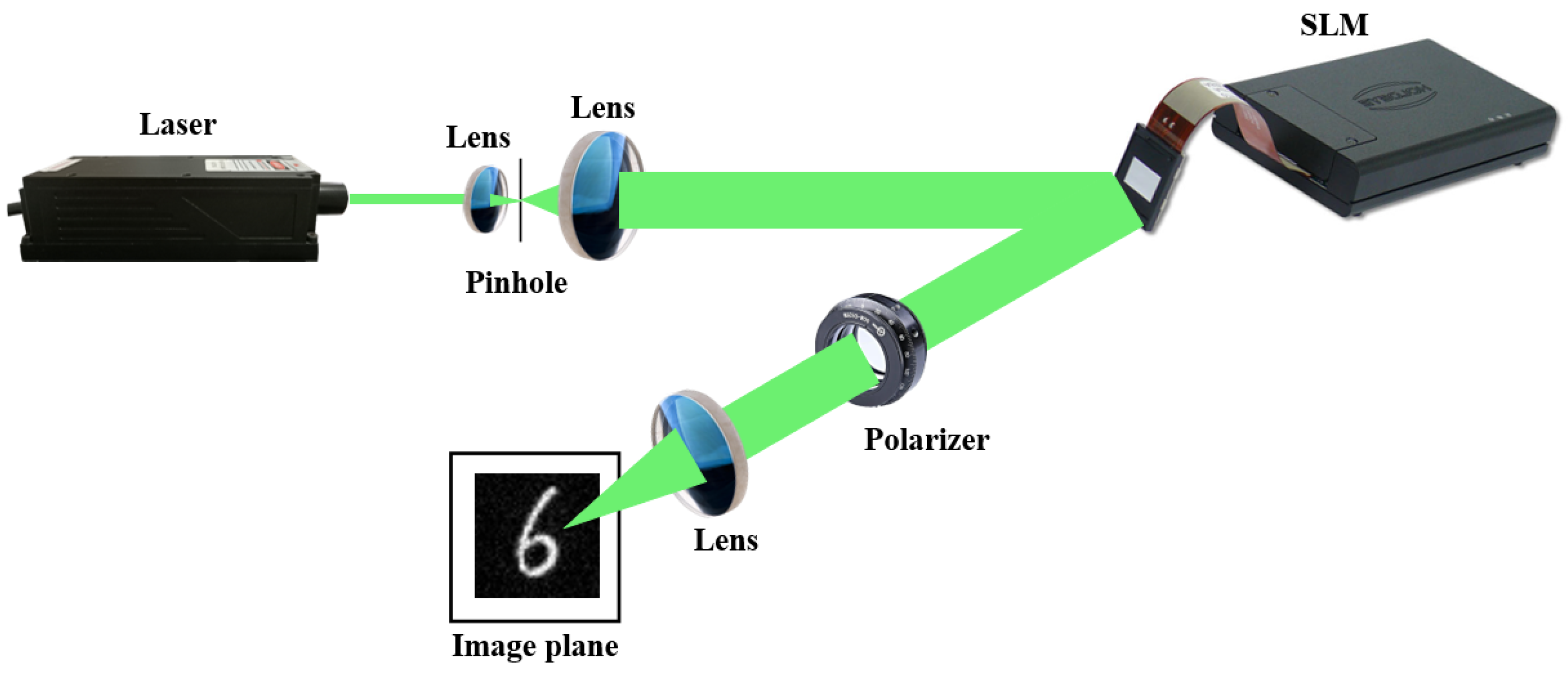
The optical setup for encoding the light wave-front with ECGH is conceptually presented in Figure 1. A beam from a 532 nm laser is collimated and expanded to obtain a plane wave, which irradiates on the SLM encoded by the computer. The encoded light wave-front is adjusted by the polarizer to focus the convex lens, and the encoded image can be displayed at the focal length. A polarizer is used to modulate the polarization angle needed by the reflective phase-modulated SLM.
An 8-bit binary gray scale image is encoded and then loaded on the SLM by the computer. The SLM can modulate the phase by converting the pixel gray level [0, 255] into a phase value of [0, 2π] under a linear transformation.
Through the optical realization setup shown in Figure 1, the corresponding principle of the computational holography, the real amplitude, and the normalized intensity of the target image are denoted as
and
where ϕSLM is the encoded image loaded. FT is a two-dimensional fast Fourier transform with a normalization ability needed to realize gradient back-propagation in deep learning. i is an imaginary unit. I is the optical intensity image with normalization by the maximum value denoted as y(ϕSLM)max. The results of calculating Equation (1) must be normalized to ensure that the calculated result conforms to the physical constraints.
Y (ϕSLM) = |FT (exp (i × ϕSLM/255 × 2π))|,
I = |y (ϕSLM)/y (ϕSLM)max|2
3. Network Structure for ECGH
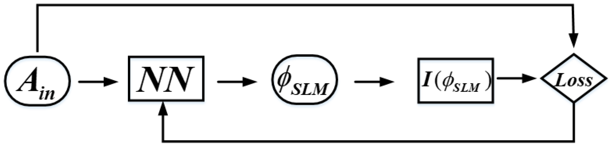
Based on Equations (1) and (2), a deep learning parameter training logic can be constructed based on the following steps:
- First, the input target light field is calculated using the neural network model to obtain the corresponding phase value.
- Second, the phase value is calculated to simulate the optical experimental results.
- Third, the target light field is compared with the simulation results using a loss function.
- Finally, the gradient of the loss value is calculated and backpropagated to update the network parameters. This is shown in Figure 2, where Ain represents the target field and NN is the neural network. Based on the superiority of this structural design, the label image is the input image, and additional label images do not need to be prepared.
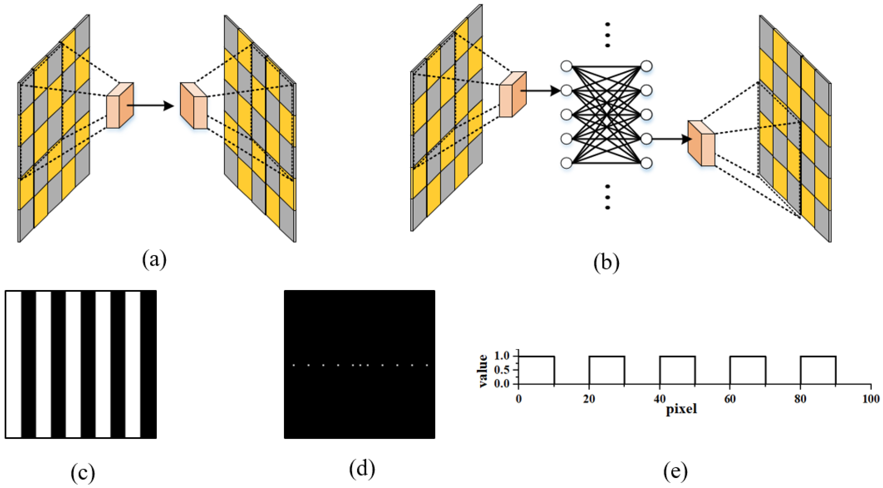
Although the U-net [28] network has shown excellent performance on many problems [29,30,31,32,33], the holograms obtained in the computational holography problem have defects that decrease the quality of the reconstruction image. Traditional convolutional neural networks rely on convolutional filters and non-linear activation functions, which means there is an assumption that the processed data are linearly separable. However, problems such as image encoding, holographic encryption, and frequency analysis are difficult to describe with linearly separable functions, and simple convolution and de-convolution are always limited to a certain area to improve the operational efficiency. The U-net cannot utilize and rewrite global information, which means that the optical image processing is very weak. The interconnected structure of the perceptron is a more efficient functional approximator that obtains more abstract feature information output [34]. A more intuitive description can be shown in Figure 3. Figure 3a gives a simplified image depicting the operations convolution and de-convolution. Figure 3c shows a series of black and white straight stripes, and the numerical distribution of the stripes is shown in Figure 3e. Figure 3d provides the result of the fast Fourier transform as shown in Figure 3c, which is a group of mirror-symmetrical points on the central axis in the frequency domain. It is difficult to obtain the independent points in the frequency domain in Figure 3d if only the spatial stripes are calculated by sampling and data blocks. This drawback can be solved by in-lining the fully connected layer, as in the structure shown in Figure 3b, which realizes the transfer and utilization of data across blocks.
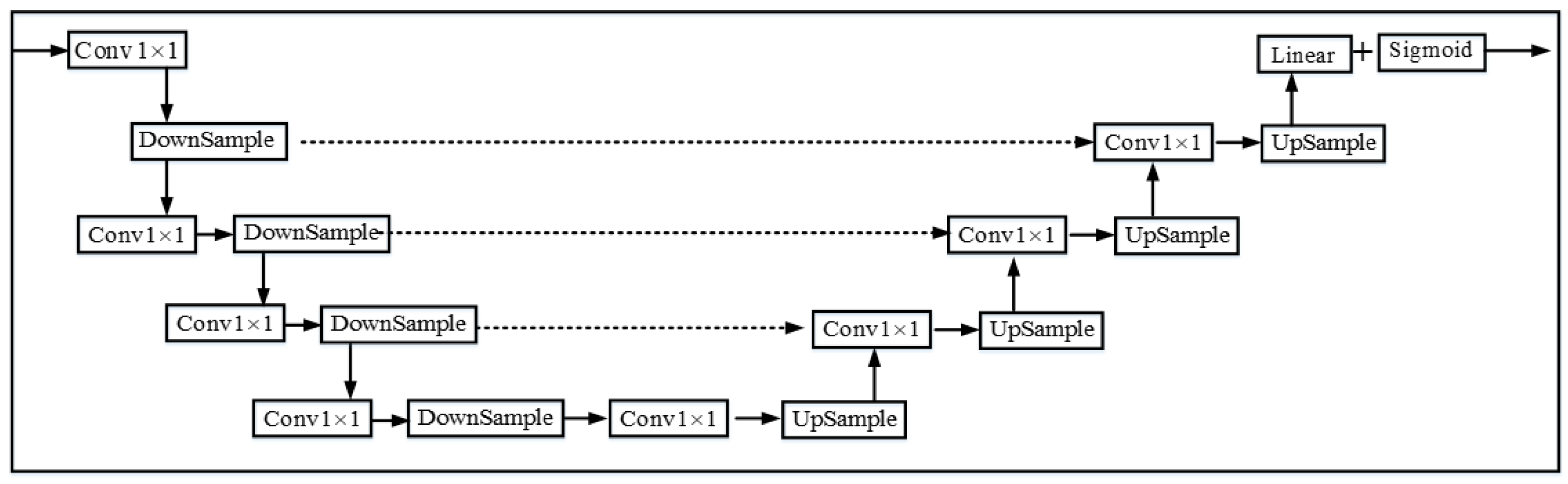
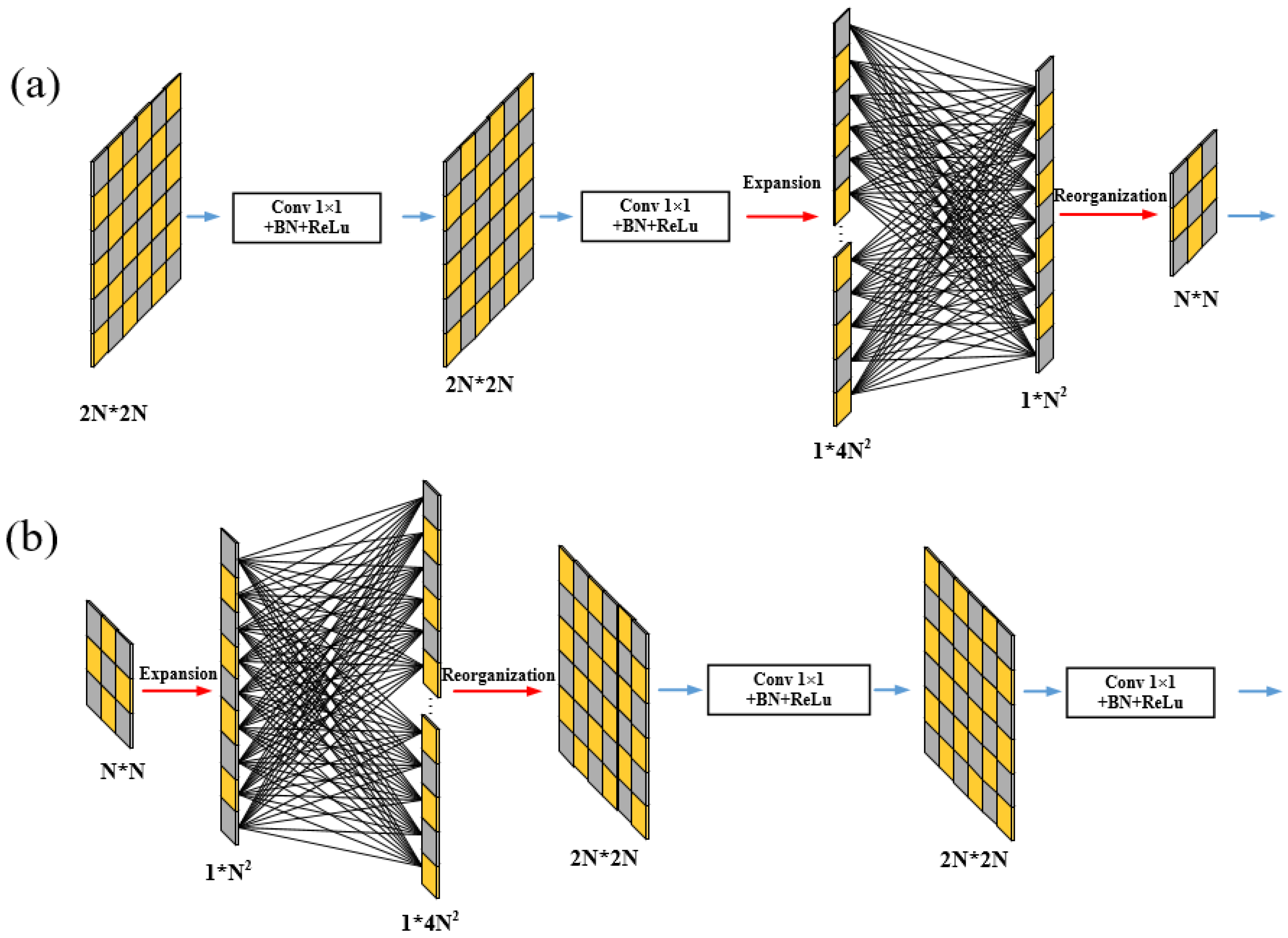
The structure of MLCNN is shown in Figure 4. The convolution kernel is a 1 × 1 convolution operation, which is used to deepen the network. “DownSample” is a down-sampling structure, and “UpSample” is an up-sampling structure, which is described later. “Linear” is a linear layer structure. “Sigmoid” is used as an activation function to constrain the output between 0 and 1. The dotted line is a bridge structure, forming a residual network to accelerate training and to reduce gradient disappearance and gradient explosion.
In order to down-sample the network information, the “DownSample” structure shown in Figure 5a is used to replace the convolution and pooling operations in the traditional neural network. Input data consist of images with sizes of 2N ∗ 2N, and then, the data are tiled into a one-dimensional vector with a size of 1 ∗ 4N2 after 1 × 1 convolution, batch normalization, and ReLu activation function. The vector is then down-sampled by the single-layer perceptron structure to obtain a one-dimensional vector of 1 ∗ N2, and the final recombination size is N ∗ N. To replace the de-convolution operation in the U-net, the “UpSample” structure shown in Figure 5b is used to up-sample the information. The input image size N ∗ N is processed by the “UpSample” structure to obtain an up-sampled image of a size 2N ∗ 2N. It is mirror-symmetrical to the “DownSample” structure.
4. Model Training
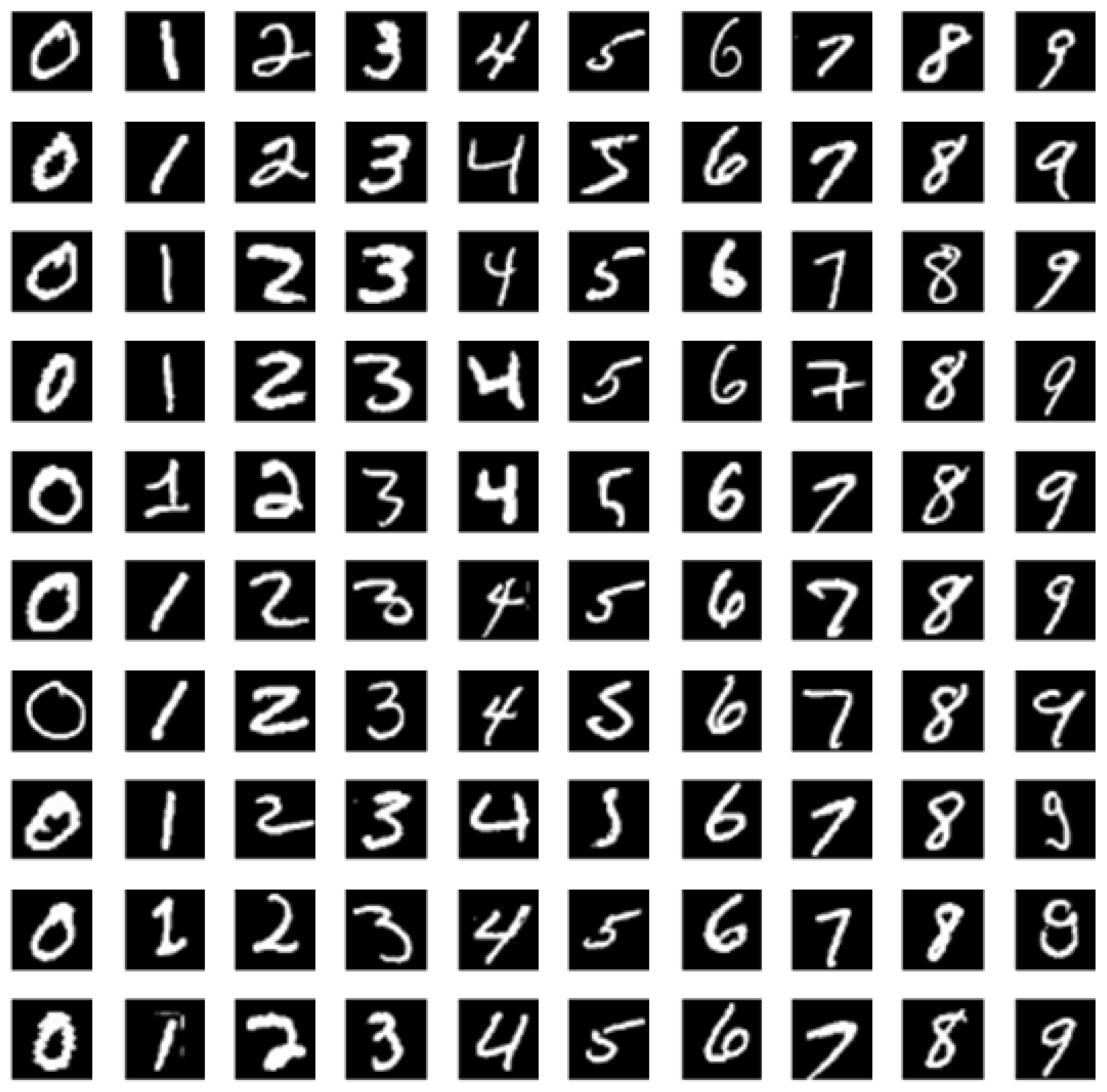
Considering the constraints of computer performance and computing time, the Mixed National Institute of Standards and Technology database (MNIST), with an image size of 48 × 48, was used to train the model. In this work, 6000 MNIST images were used and split into a training set and a test set according to the ratio of 5:1. The MNIST dataset consists of handwritten digits 0–9 collected from census employees and high school students, each with a different style. Figure 6 shows a partial representation of the MNIST data.
The initial assignment of network parameters is random. In order to obtain parameters that match the computational holography problem, the network parameters need to be optimized. We use the Adam optimizer and the mean square loss function to promote the optimization process:
where x and y are the computer generated image and label image, respectively; aij and bij are the corresponding pixels of the image; and m and n are the number of pixels in the length/width of the image. The parameter settings of the Adam optimizer are given in Table 1, where β1 and β2 are hyper parameters, and є is a stabilization factor.
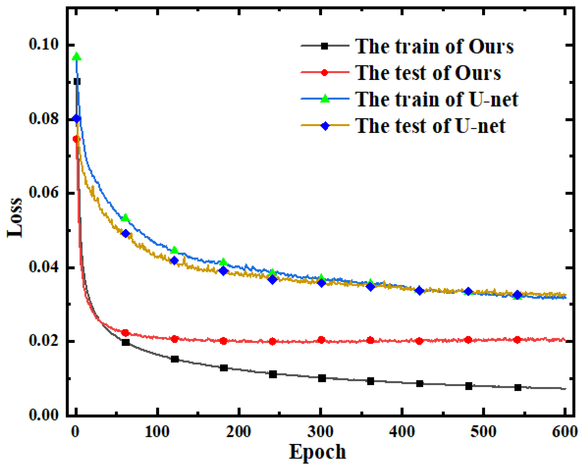
The network was trained for 600 epochs on the platform of the Pytorch framework. The comparison of the U-net model parameters with ours is given in Table 2. Although our method requires more hidden layers, it no longer requires a large number of convolution kernels to complete information mining, and therefore, the total number of parameters is fewer. Compared with the conventional U-net network using 31,042,369 parameters, the MLCNN network contains 9,720,580 parameters, which account for only 31% of the U-net network parameters. Simultaneously, the mean square deviation decreases from 0.03181 to 0.00731. To investigate the performance of this MLCNN design further, the training results are given in Figure 7. In Figure 7, the results of the loss function for the training set and the test set by the MLCNN network and the U-net network are shown simultaneously for comparison. To investigate the computing efficiency of MLCNN network, a common computer with a CPU processor (Intel i5) and a GPU (Nvidia GTX 1060) is employed to complete the training. The results show that 38 ms and 9.8 ms are needed to finish the MLCNN network training and the phase-only holographic image generation for one frame, respectively. For comparison, similar work is additionally conducted by both the U-net network and the GS iterative method. The corresponding computing times used for the phase-only holographic image generation are 13.5 ms and 0.62 s for one frame. The results show that the MLCNN network has faster optimization speed and higher accuracy than either the U-net network or the GS algorithm.
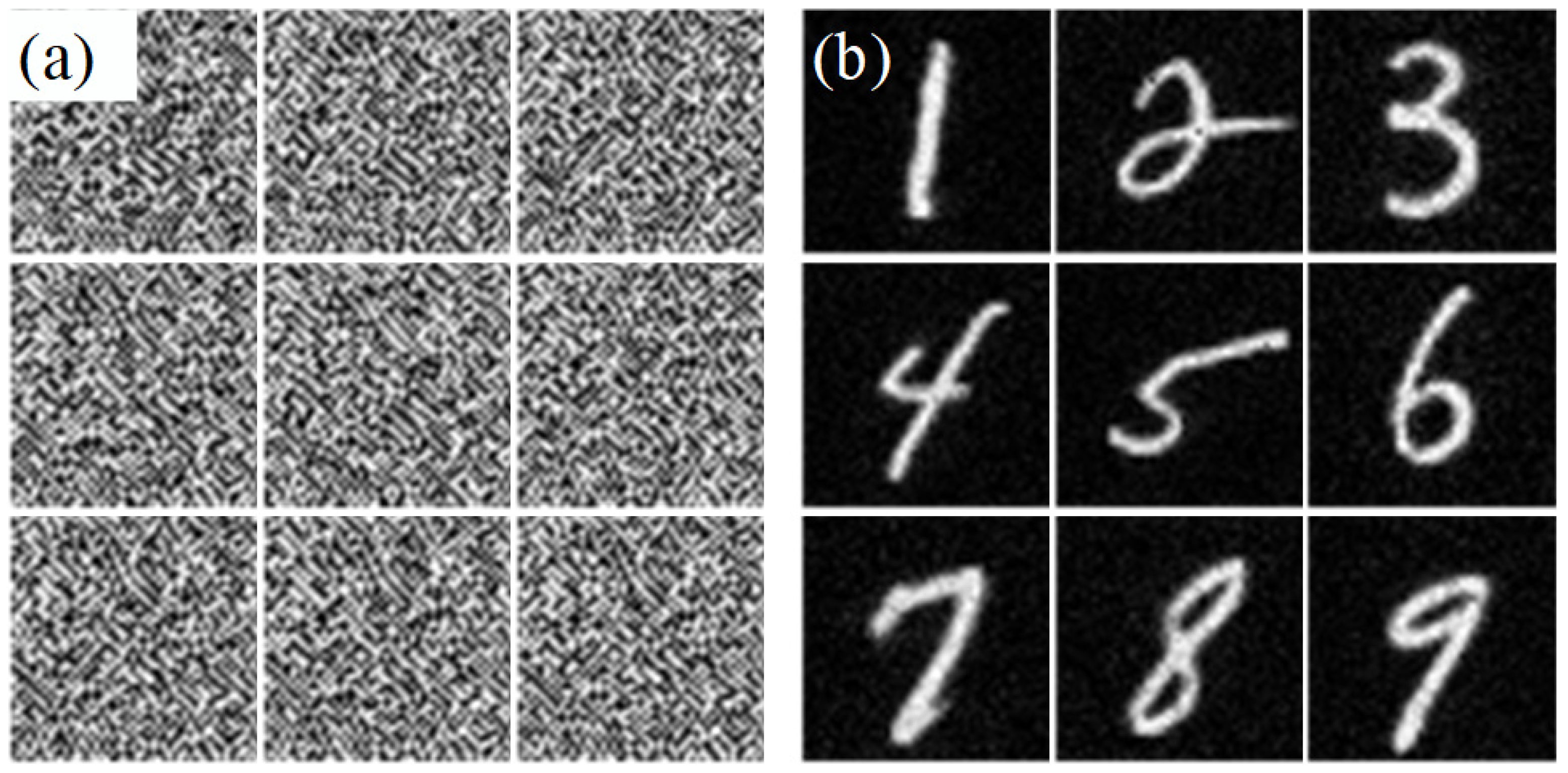
We use the network parameters with an epoch of 600 to generate the holographic images and have analyzed the test set. Part of the results is shown in Figure 8. Figure 8a shows phase-type holographic images of the numbers “1–9” obtained using this method, and Figure 8b shows the computer-simulated results of these holographic images.
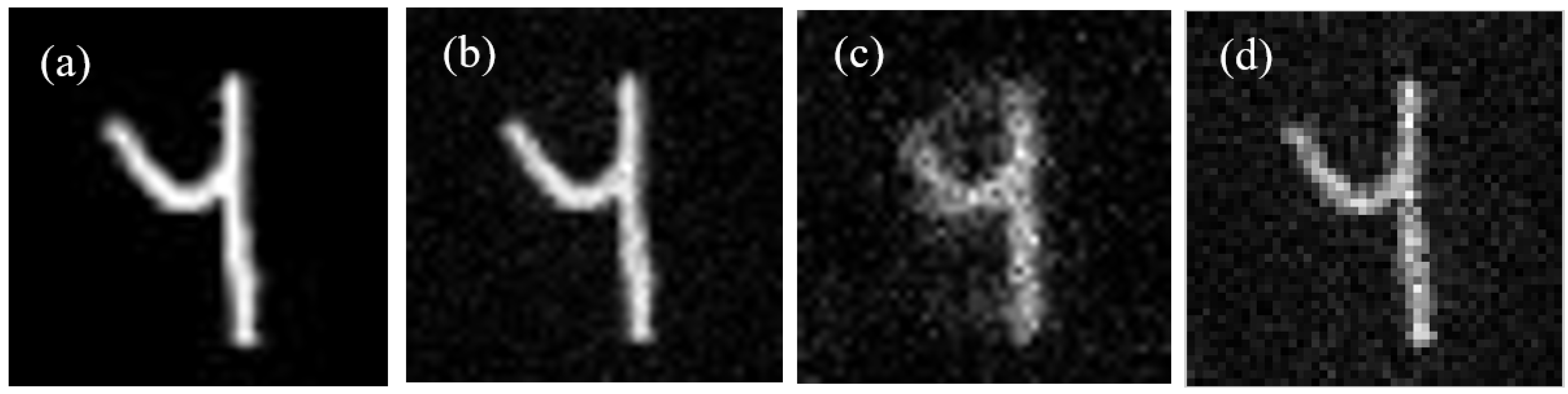
In order to intuitively observe the differences of the CGH images obtained using different methods, the reconstruction results obtained by them are shown in Figure 9. Figure 9a is an original image of the handwritten numeral “4”. Figure 9b is the reconstructed result of the computational hologram obtained using the MLCNN network. Figure 9c is the reconstructed result of the computational hologram obtained using the U-net network. Figure 9d is the reconstructed result of the computer-generated hologram obtained using the GS algorithm. The simulated reproduction result of the MLCNN network is very close to the target image, with higher reconstruction accuracy and lower noise interference.
5. Stability Analysis
The Structural Similarity (SSIM) [35] is rescued to objectively evaluate the difference in quality between the images reconstructed using the MLCNN deep learning methods and the original label images. Although the mean squared error and the peak signal-to-noise ratio have been widely used because of their ease of use and their well-defined physical meaning, these two functions do not match human visual perception. The SSIM in Equation (4) provides a more effective objective criterion by comprehensively evaluating image brightness, contrast, and structure.
where x and y are the two normalized images to be calculated; μx and μy are the mean values of the two images; σx and σy are the standard deviations; σxy is the covariance of the two images of x and y; and c1 = (k1L)2 and c2 = (k2L)2 are two constants with k1 = 0.01, k2 = 0.03, and L = 255 for an 8-bit binary image. The value of the SSIM is between 0 and 1. The closer the SSIM value is to 1, the higher the image similarity. When the two images are identical, the structural similarity is 1. In order to evaluate the quality of the generated images more objectively, the intensity value for all pixels in images are normalized to [0, 1], and the MATLAB software is used to calculate each group of images.
SSIM (x,y) = (2 × μxμy + c1) × (2 × σxy + c2)/(μx2 + μy2 + c1)/(σx2 + σy2 + c2)
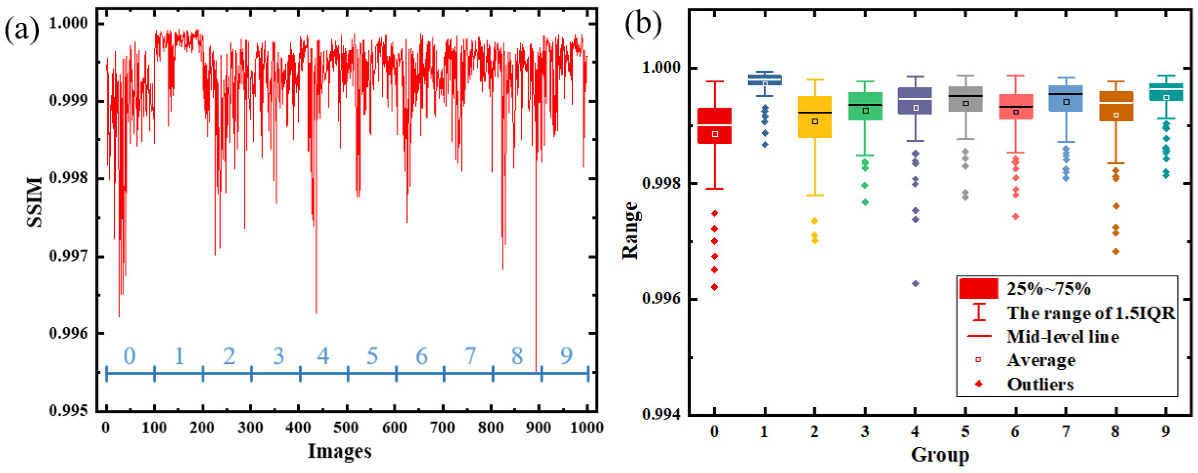
Figure 10a shows the structural similarity curve between the simulated reproduction of the phase map generated by the MLCNN network and the target light field. Among the 1000 test images, each 100 is a group corresponding to the handwritten numbers “0–9”. It is obvious that the digital “1” has a higher SSIM value due to the simpler structure. Although there are some fluctuations in the quality of the reconstructed image, it can still give a high-quality phase map. The boxplot can better reflect the distribution characteristics of the data. The reconstructed images are grouped by corresponding numbers, and the drawn boxplot is shown in Figure 10b. Among these, the box size reflects the data distribution between 25% and 75% after the data are arranged in ascending order. Between the upper and lower bounds are data within 1.5 times the interquartile range (IQR). Only a small part of the data are outliers, and the overall structural similarity of the images is higher than 0.998. Therefore, the quality of the holograms generated by the MLCNN network is stable.
6. Conclusions
In this paper, we proposed a non-iterative deep learning model, MLCNN, for generating ECGH images. Compared with the traditional U-net network [21,22] and the GS algorithm [17], our method can achieve faster computation speeds in hologram generation. High-quality and stable computational holographic images were successfully obtained using the ECGH method. A major feature of the MLCNN network structure is that it can calculate the cross-region exchange of data. This is optimal for complex optical functions such as Fourier transforms that require manipulation of global information. The results show that the MLCNN network structure is more suitable for the optical domain than the classical U-net network, especially for holography generation and reconstruction work.
Virtual reality (VR) and augmented reality (AR) are currently hot topics in display technology and application. However, conventional technologies in VR and AR employ micro-displays to load images, which can cause visual fatigue when they are used for extended periods of time. Benefiting from the ability to reproduce three-dimensional scenes perfectly, computational holography can prevent visual fatigue. This ECGH method is expected to ease the huge CGH computing load and to improve the quality of the computational holography images.
Author Contributions
Conceptualization, X.X.; Data curation, X.W.; Formal analysis, X.W.; Funding acquisition, H.W.; Investigation, X.W.; Validation, W.L. and Y.S.; Writing—original draft, X.W.; Writing—review & editing, X.X. All authors have read and agreed to the published version of the manuscript.
Funding
Natural Science Foundation of Shandong Province, China (ZR2019MD023) and Fundamental Research Funds for the Central Universities of China (15CX05033A).
Institutional Review Board Statement
Not applicable.
Informed Consent Statement
Not applicable.
Data Availability Statement
Not applicable.
Conflicts of Interest
The authors declare no conflict of interest.
References
- Goodman, J.W.; Lawrence, R.W. Digital image formation from electronically detected holograms. Appl. Phys. Lett. 1967, 11, 77–79. [Google Scholar] [CrossRef]
- Poon, T.C.; Liu, J.P. Introduction to Modern Digital Holography with MATLAB; Cambridge University Press: Cambridge, UK, 2014. [Google Scholar]
- Xu, X.; Ma, T.; Jiao, Z.; Xu, L.; Dai, D.; Qiao, F.; Poon, T.-C. Novel Generalized Three-Step Phase-Shifting Interferometry with a Slight-Tilt Reference. Appl. Sci. 2019, 9, 5015. [Google Scholar] [CrossRef] [Green Version]
- Grier, D.G.; Roichman, Y. Holographic optical trapping. Appl. Opt. 2006, 45, 880–887. [Google Scholar] [CrossRef] [PubMed] [Green Version]
- He, M.R.; Liang, Y.S.; Bianco, P.R.; Wang, Z.J.; Yun, X.; Cai, Y.N.; Feng, K.; Lei, M. Trapping performance of holographic optical tweezers generated with different hologram algorithms. AIP Adv. 2021, 11, 035130–035139. [Google Scholar] [CrossRef]
- Yang, W.; Yuste, R. Holographic imaging and photostimulation of neural activity. Curr. Opin. Neurobiol. 2018, 50, 211–221. [Google Scholar] [CrossRef]
- Yang, S.; Papagiakoumou, E.; Guillon, M.; De Sars, V.; Tang, C.-M.; Emiliani, V. Three-dimensional holographic photostimulation of the dendritic arbor. J. Neural Eng. 2011, 8, 046002–046010. [Google Scholar] [CrossRef]
- Gao, C.; Liu, J.; Li, X.; Xue, G.; Jia, J.; Wang, Y. Accurate compressed look up table method for CGH in 3D holographic display. Opt. Express 2015, 23, 33194–33204. [Google Scholar] [CrossRef]
- Leseberg, D.; Frère, C. Computer-generated holograms of 3-D objects composed of tilted planar segments. Appl. Opt. 1988, 27, 3020–3024. [Google Scholar] [CrossRef]
- Park, J.-H. Recent progress in computer-generated holography for three-dimensional scenes. J. Inf. Disp. 2017, 18, 1–12. [Google Scholar] [CrossRef] [Green Version]
- Wakunami, K.; Hsieh, P.-Y.; Oi, R.; Senoh, T.; Sasaki, H.; Ichihashi, Y.; Okui, M.; Huang, Y.-P.; Yamamoto, K. Projection-type see-through holographic three-dimensional display. Nat. Commun. 2016, 7, 12954. [Google Scholar] [CrossRef] [Green Version]
- Pirone, D.; Sirico, D.G.; Miccio, L.; Bianco, V.; Mugnano, M.; Ferraro, P.; Memmolo, P. Speeding up reconstruction of 3D tomograms in holographic flow cytometry via deep learning. Lab Chip 2022, 22, 793–804. [Google Scholar] [CrossRef] [PubMed]
- Yolalmaz, A.; Yüce, E. Effective bandwidth approach for the spectral splitting of solar spectrum using diffractive optical elements. Opt. Express 2020, 28, 12911–12921. [Google Scholar] [CrossRef] [PubMed]
- Gün, B.N.; Yüce, E. Wavefront shaping assisted design of spectral splitters and solar concentrators. Sci. Rep. 2021, 11, 2825. [Google Scholar] [CrossRef] [PubMed]
- Moon, S.; Lee, C.-K.; Nam, S.-W.; Jang, C.; Lee, G.-Y.; Seo, W.; Sung, G.; Lee, H.-S.; Lee, B. Augmented reality near-eye display using Pancharatnam-Berry phase lenses. Sci. Rep. 2019, 9, 6616. [Google Scholar] [CrossRef]
- Cem, A.; Hedili, M.K.; Ulusoy, E.; Urey, H. Foveated near-eye display using computational holography. Sci. Rep. 2020, 10, 14905. [Google Scholar] [CrossRef]
- Gerchberg, R.W.; Saxton, W.O. Phase determination for image and diffraction plane pictures in the electron microscope. Optik 1971, 35, 237–246. [Google Scholar]
- Chang, C.; Xia, J.; Yang, L.; Lei, W.; Yang, Z.; Chen, J. Speckle-suppressed phase-only holographic three-dimensional display based on double-constraint Gerchberg-Saxton algorithm. Appl. Opt. 2015, 54, 6994–7001. [Google Scholar] [CrossRef]
- Lohmann, A.W.; Paris, D.P. Binary Fraunhofer Holograms, Generated by Computer. Appl. Opt. 1967, 6, 1739–1748. [Google Scholar] [CrossRef]
- Lin, X.; Rivenson, Y.; Yardimci, N.T.; Veli, M.; Luo, Y.; Jarrahi, M.; Ozcan, A. All-optical machine learning using diffractive deep neural networks. Science 2018, 361, 1004–1008. [Google Scholar] [CrossRef] [Green Version]
- Lee, J.; Jeong, J.; Cho, J.; Yoo, D.; Lee, B. Deep neural network for multi-depth hologram generation and its training strategy. Opt. Express 2020, 28, 27137–27154. [Google Scholar] [CrossRef]
- Horisaki, R.; Takagi, R.; Tanida, J. Deep-learning-generated holography. Appl. Opt. 2018, 57, 3859–3863. [Google Scholar] [CrossRef] [PubMed]
- Shi, L.; Li, B.; Kim, C.; Kellnhofer, P.; Matusik, W. Towards real-time photorealistic 3D holography with deep neural networks. Nature 2021, 591, 234–239. [Google Scholar] [CrossRef] [PubMed]
- Peng, Y.; Choi, S.; Padmanaban, N.; Wetzstein, G. Neural holography with camera-in-the-loop training. ACM Trans. Graph. 2020, 39, 185. [Google Scholar] [CrossRef]
- Balasubramaniam, G.M.; Wiesel, B.; Biton, N.; Kumar, R.; Kupferman, J.; Arnon, S. Tutorial on the Use of Deep Learning in Diffuse Optical Tomography. Electronics 2022, 11, 305. [Google Scholar] [CrossRef]
- Kim, G.; Kim, J.; Choi, W.J.; Kim, C.; Lee, S. Integrated deep learning framework for accelerated optical coherence tomography angiography. Sci. Rep. 2022, 12, 1289. [Google Scholar] [CrossRef] [PubMed]
- Choy, K.C.; Li, G.; Stamer, W.D.; Farsiu, S. Open-source deep learning-based automatic segmentation of mouse Schlemm’s canal in optical coherence tomography images. Exp. Eye Res. 2021, 214, 108844. [Google Scholar] [CrossRef] [PubMed]
- Ronneberger, O.; Fischer, P.; Brox, T. U-Net: Convolutional Networks for Biomedical Image Segmentation. In Medical Image Computing and Computer-Assisted Intervention 2015; Navab, N., Hornegger, J., Wells, W.M., Frangi, A.F., Eds.; Springer International Publishing: Cham, Switzerland, 2015; pp. 234–241. [Google Scholar] [CrossRef] [Green Version]
- Du, G.; Cao, X.; Liang, J.; Chen, X.; Zhan, Y. Medical image segmentation based on u-net: A review. J. Imaging Sci. Technol. 2020, 64, 20508-1–20508-12. [Google Scholar] [CrossRef]
- Chen, Z.; Wang, C.; Li, J.; Xie, N.; Han, Y.; Du, J. Reconstruction Bias U-Net for Road Extraction From Optical Remote Sensing Images. IEEE J. Sel. Top. Appl. Earth Obs. Remote Sens. 2021, 14, 2284–2294. [Google Scholar] [CrossRef]
- Li, L.; Jia, T.; Li, T.J.L. Optical Coherence Tomography Vulnerable Plaque Segmentation Based on Deep Residual U-Net. Rev. Cardiovasc. Med. 2019, 20, 171–177. [Google Scholar] [CrossRef]
- Chen, T.; Lu, T.; Song, S.; Miao, S.; Gao, F.; Li, J. A deep learning method based on U-Net for quantitative photoacoustic imaging. In Proceedings of the Photons Plus Ultrasound: Imaging and Sensing 2020, San Francisco, CA, USA, 2–5 February 2020. [Google Scholar] [CrossRef]
- Wang, X.; Wei, H. Cryptanalysis of compressive interference-based optical encryption using a U-net deep learning network. Opt. Commun. 2022, 507, 27641. [Google Scholar] [CrossRef]
- Lin, M.; Chen, Q.; Yan, S. Network in network. arXiv 2013, arXiv:1312.4400. [Google Scholar]
- Wang, Z.; Bovik, A.C.; Sheikh, H.R.; Simoncelli, E.P. Image Quality Assessment: From Error Visibility to Structural Similarity. IEEE Trans. Image Process. 2004, 13, 600–612. [Google Scholar] [CrossRef] [PubMed] [Green Version]
Figure 1.
Optical setup of ECGH reconstruction.

Figure 2.
Network training logic.

Figure 3.
Advantages of MLCNN structure with linear cross layer. (a) Without linear layer structure; (b) with linear layer structure; (c) fringe image; (d) fast Fourier transform result; (e) numerical distribution.
Figure 3.
Advantages of MLCNN structure with linear cross layer. (a) Without linear layer structure; (b) with linear layer structure; (c) fringe image; (d) fast Fourier transform result; (e) numerical distribution.

Figure 4.
MLCNN network structure.

Figure 5.
Sampling method: (a) DownSample structure; (b) UpSample structure.

Figure 6.
Some handwritten digits.

Figure 7.
The loss curve comparison for U-net and MLCNN.

Figure 8.
Generated holograms and reproduced images. (a) Phase-type hologram generated by MLCNN; (b) reconstructed images.
Figure 8.
Generated holograms and reproduced images. (a) Phase-type hologram generated by MLCNN; (b) reconstructed images.

Figure 9.
Comparison of reproduction results. (a) Original image; (b) MLCNN reconstruction; (c) U-net reconstruction; and (d) GS algorithm reconstruction.
Figure 9.
Comparison of reproduction results. (a) Original image; (b) MLCNN reconstruction; (c) U-net reconstruction; and (d) GS algorithm reconstruction.

Figure 10.
Structural similarity of ECGH reconstructed images: (a) curve plot; (b) box plot.


Table 1.
Optimizer parameter table.
| Optimizer | Learning Rate | (β1, β2) | є |
|---|---|---|---|
| Adam | 0.01 | (0.9, 0.999) | 10−8 |
Table 2.
Model parameter comparison.
| Model | Input/Output Size | Layers | Total Params | Mean Square Loss |
|---|---|---|---|---|
| U-net | 48 × 48 | 62 | 31,042,369 | 0.03181 |
| Ours | 48 × 48 | 82 | 9,720,580 | 0.00731 |
Publisher’s Note: MDPI stays neutral with regard to jurisdictional claims in published maps and institutional affiliations. |
© 2022 by the authors. Licensee MDPI, Basel, Switzerland. This article is an open access article distributed under the terms and conditions of the Creative Commons Attribution (CC BY) license (https://creativecommons.org/licenses/by/4.0/).
Share and Cite
MDPI and ACS Style
Xu, X.; Wang, X.; Luo, W.; Wang, H.; Sun, Y. Efficient Computer-Generated Holography Based on Mixed Linear Convolutional Neural Networks. Appl. Sci. 2022, 12, 4177. https://0-doi-org.brum.beds.ac.uk/10.3390/app12094177
AMA Style
Xu X, Wang X, Luo W, Wang H, Sun Y. Efficient Computer-Generated Holography Based on Mixed Linear Convolutional Neural Networks. Applied Sciences. 2022; 12(9):4177. https://0-doi-org.brum.beds.ac.uk/10.3390/app12094177
Chicago/Turabian StyleXu, Xianfeng, Xinwei Wang, Weilong Luo, Hao Wang, and Yuting Sun. 2022. "Efficient Computer-Generated Holography Based on Mixed Linear Convolutional Neural Networks" Applied Sciences 12, no. 9: 4177. https://0-doi-org.brum.beds.ac.uk/10.3390/app12094177
Note that from the first issue of 2016, this journal uses article numbers instead of page numbers. See further details here.