
Aero-Engine Remaining Useful Life Estimation Based on CAE-TCN Neural Networks


1
Institute of Automation, Chinese Academy of Sciences, Beijing 100190, China
2
School of Mechanical Engineering & Automation, Beihang University, Beijing 100191, China
3
School of Automation, Beijing Institute of Technology, Beijing 100081, China
*
Authors to whom correspondence should be addressed.
Appl. Sci. 2023, 13(1), 17; https://0-doi-org.brum.beds.ac.uk/10.3390/app13010017
Submission received: 18 October 2022
/
Revised: 6 December 2022
/
Accepted: 10 December 2022
/
Published: 20 December 2022
(This article belongs to the Special Issue New Trends in Machine Diagnostic and Condition Monitoring)
Abstract
:With the rapid growth of the aviation fields, the remaining useful life (RUL) estimation of aero-engine has become the focus of the industry. Due to the shortage of existing prediction methods, life prediction is stuck in a bottleneck. Aiming at the low efficiency of traditional estimation algorithms, a more efficient neural network is proposed by using Convolutional Neural Networks (CNN) to replace Long-Short Term Memory (LSTM). Firstly, multi-sensor degenerate information fusion coding is realized with the convolutional autoencoder (CAE). Then, the temporal convolutional network (TCN) is applied to achieve efficient prediction with the obtained degradation code. It does not depend on the iteration along time, but learning the causality through a mask. Moreover, the data processing is improved to further improve the application efficiency of the algorithm. ExtraTreesClassifier is applied to recognize when the failure first develops. This step can not only assist labelling, but also realize feature filtering combined with tree model interpretation. For multiple operation conditions, new features are clustered by K-means++ to encode historical condition information. Finally, an experiment is carried out to evaluate the effectiveness on the Commercial Modular Aero-Propulsion System Simulation (CMAPSS) datasets provided by the National Aeronautics and Space Administration (NASA). The results show that the proposed algorithm can ensure high-precision prediction and effectively improve the efficiency.
1. Introduction
The aero-engine, as the main power source, is the core component of various spacecraft. Its safety, reliability and economy are the focus of aero-engine manufacturers, maintenance plants and other relevant departments [1]. As an important reference index to achieve preventive maintenance, it is of great significance to accurately estimate the RUL of the aero-engine. However, the working environment of the engine is harsh (high temperature, high pressure, etc.), and existing prediction methods often cannot meet the industrial demand.
With the rise of artificial intelligence, a new maintenance concept known as Condition Based Maintenance (CBM) has been seen a lot in recent research. Compared with traditional maintenance measures like scheduled maintenance, CBM is more efficient and costs less time [2,3]. This situation is also reflected in the study of the RUL estimation. Traditional prediction methods are built based on the physical mechanism of equipment or system degradation [4], such as particle filter [5], Eyring model [6], Weibull distribution [7], etc. This shows an over-reliance on expert knowledge. Besides, for aero-engine, obtaining the proper physical and mathematical model is challenging for the actual industrial environment. In contrast, CBM attempts to detect the degradation law in a data-driven way [8,9]. It takes monitoring data collected by the sensor as input. Then, the mapping between data and labels could be learned with some models. Finally, the RUL estimation could be realized by this trained model. Hence, the RUL estimation based on CBM is easier to implement in the actual industrial environment. With the increase in the amount of data and the continuous learning of the model, the prediction effect is more accurate. The typical data-driven methods include Support Vector Regression (SVR) [10] and Hidden Markov models [11]. In recent years, artificial neural networks have been introduced to replace feature extraction in the data-driven method, such as Multi-layer Perceptron (MLP) [12], Deep Belief Networks (DBN) [13], CNN [14], Recurrent Neural Networks (RNN) [15], LSTM [16], etc. LSTM in particular, a variant of RNN, is one of the most popular neural networks to solve time series problems. It could effectively alleviate the gradient vanishing which often occurs in RNN training. However, LSTM needs to iterate in time steps, which cannot be parallel. This means that the prediction model with the LSTM layer is inefficient in the face of real-time prediction of big time-series data. Recently, one-dimensional CNN has been applied to deal with sequential problems and achieved good results in some studies [17]. Compared with LSTM, CNN can be parallelized effectively, benefitting by its convolution structure.
In the paper, a more efficient neural network is proposed to estimate the RUL with CAE and TCN. There is no LSTM layer in the model structure, instead of the convolution layer. Therefore, the algorithm can greatly improve the prediction efficiency of the RUL estimation without losing the prediction accuracy. In addition, a state discriminator based on ExtraTreesClassifier is used to label the RUL in the data preprocessing. Combined with tree model interpretation, the automatic filtering of input features is realized.
The rest of this paper is structured as follows. Section 2 defines the structure of the proposed prediction model. In addition, the procedure of the whole RUL estimation is described. ExtraTreesClassifier is used as the state detector and K-means++ as the new operational features extractor. Then, in Section 3, an experiment is described with the CMAPSS datasets. The results are compared with widely used prediction algorithms, vanilla LSTM and one-dimensional CNN. Finally, a summary of this paper is provided with conclusions in Section 4.
2. Methodology
A more efficient neural network is proposed to estimate the RUL with CAE and TCN. In this section, CAE, TCN and the proposed model structure have been introduced and explained in detail.
2.1. CAE
Autoencoder (AE) is an artificial neural network to realize data representation learning. At first, AE was studied to solve the “encoder problem” in representation learning. In 1985, David H. Ackley, Geoffrey E. Hinton and Terrence J. Sejnowski first tried the AE algorithm on the Boltzmann machine. Its effect of representation learning was discussed [18]. After the backpropagation (BP) was proposed, AE was studied as one of the implementations of BP [19]. Until 1987, AE was formally proposed in a study by Yann LeCun [20]. In the research, an AE was constructed by MLP to reduce data noise. In addition, the research on data dimensionality reduction using MLP AE also received attention [21]. The schematic of AE is shown in Figure 1.
AE can achieve self-supervised learning with its symmetrical model structure: encoder and decoder [22]. The encoder compresses the high-dimensional input into a latent spatial representation (Formula (1)), and then restores the low-dimensional representation to the high-dimensional output which is similar to the input (Formula (2)).
where is the nonlinear activation function, and represents the weights and bias of the encoder and and represents the decoder. It is a learning algorithm of connectionist model based on the dimensionality reduction problem of neural networks.
Due to the reason that the dimension of is generally much smaller than , AE is widely used for dimensionality reduction. Moreover, the encoder could be used to provide efficient representation of inputs for other tasks.
The traditional AE generally uses fully connected layers (FC). Hence, there are too many redundant parameters introduced in the model. In addition, spatial information of the input cannot be effectively learned. As a result, the learned representation is often not good enough for multi-dimensional data. By replacing the FC layer with the convolution layer, CAE can effectively solve the above problems. The principle of CAE is the same as AE. It could downsample the input to provide a smaller dimensional potential representation. The spatial information can be effectively learned through convolution, and the model parameters can be reduced at the same time.
2.2. TCN
TCN is a variant of one-dimensional CNN. CNN firstly proposed by LeCun for image classification [23]. It is widely used for extracting spatial features from high-dimensional data. By imitating the visual perception mechanism of creature, CNN is good at identifying simple patterns in the data [24]. Then, through multi-layer stacking, these simple patterns are combined into higher level features [25]. As a kind of feed-forward neural network, its artificial neurons can respond to a part of the surrounding cells in the coverage range, which has excellent performance for large-scale image processing. With one-dimensional filter kernels, CNN could handle sequential data such as text, speech and time series. One-dimensional CNN is shown in Figure 2.
The main difference is the dimension of kernels between two-dimensional and one-dimensional CNN. Due to the local connectivity, one-dimensional CNN performs well in dealing with time patterns. For some problems, especially the time series analysis task of sensor data, it can replace RNN and be faster.
The input of one-dimensional CNN is as follows (Formula (3)):
where N represents the sequence’s length. The physical meaning of convolution operation is the linear superposition of inputs in a certain region. Hence, the mathematical expression of convolution operation could be obtained (Formulas (4) and (5)).
where is the transpose of filter kernel , “…” stands for matrix multiplication and and b are the nonlinear activation function and bias, respectively.
Based on one-dimensional CNN, causal convolution is proposed [26]. Causal convolution is a one-way structure, which is a model with time constraints. The output at the current time is only related to the earlier elements in the previous layer. However, the history that could be looked back to by causal convolution is limited. The length of time that can be modeled is limited by the kernel size. Longer dependencies require a linear stacking of many one-dimensional CNN layers. To increase the receptive field of the convolution kernel, dilated convolution is used. With the dilation factor , the convolutions allow for an exponentially large receptive field. The following is the definition of the dilated convolution operation on element of the one-dimensional sequence (Formula (6)):
where means the dilation factor, denotes the filter size and describes the historical direction.
TCN is a combination of dilated convolution and causal convolution. In addition, skip-connection of Deep residual network and batch normalization are applied to prevent overfitting. TCN is shown in Figure 3.
2.3. Proposed RUL Estimation Model
As a commonly used time series prediction model, LSTM realizes the learning of time data by maintaining hidden variables with time steps. Precisely because of this, the model with LSTM could only learn iteratively along the time dimension. Thus, the model cannot be effectively parallelized when processing long time series data. In order to solve this problem, a novel RUL estimation model is proposed. It realizes the prediction of time series by replacing LSTM with CNN. It can improve the application efficiency while ensuring the prediction ability. The architecture of the proposed RUI estimation model is illustrated in Figure 4.
There are two parts in the model, CAE and TCN. Firstly, CAE is used to realize learning of the degradation trend of the engine. Multi-dimensional time series are flattened as a single dimensional degenerate sequence by the encoder. Then, TCN is applied to achieve the RUL estimation. In the prediction phase, the multi-dimensional data is used as trained CAE input to realize degenerate coding. After encoding, the obtained degenerate sequence is used to predict the RUL through TCN. Data slicing and data stacking can lead to massive loss of information. CAE is used to keep the spatial information unchanged instead of data stacking, and extracts the information in a gentle way in the convolution layer. The feature extraction is realized by multiple convolution kernel, and then the dimension is reduced slowly combined with MaxPooling layers. In addition, the batch normalization layer is added to reduce overfitting. As shown in Figure 4, a thick cube is extracted first, and then a longer cuboid is extracted. This design is intended to aid CAE in better coding. This structure can effectively extract degraded features, while ensuring the ability of temporal features extraction. Considering the input of CAE, a sliding window is used. To simplify the calculation, the window width is the same as the dimension of the input data.
2.4. Complete RUL Prediction Algorithm
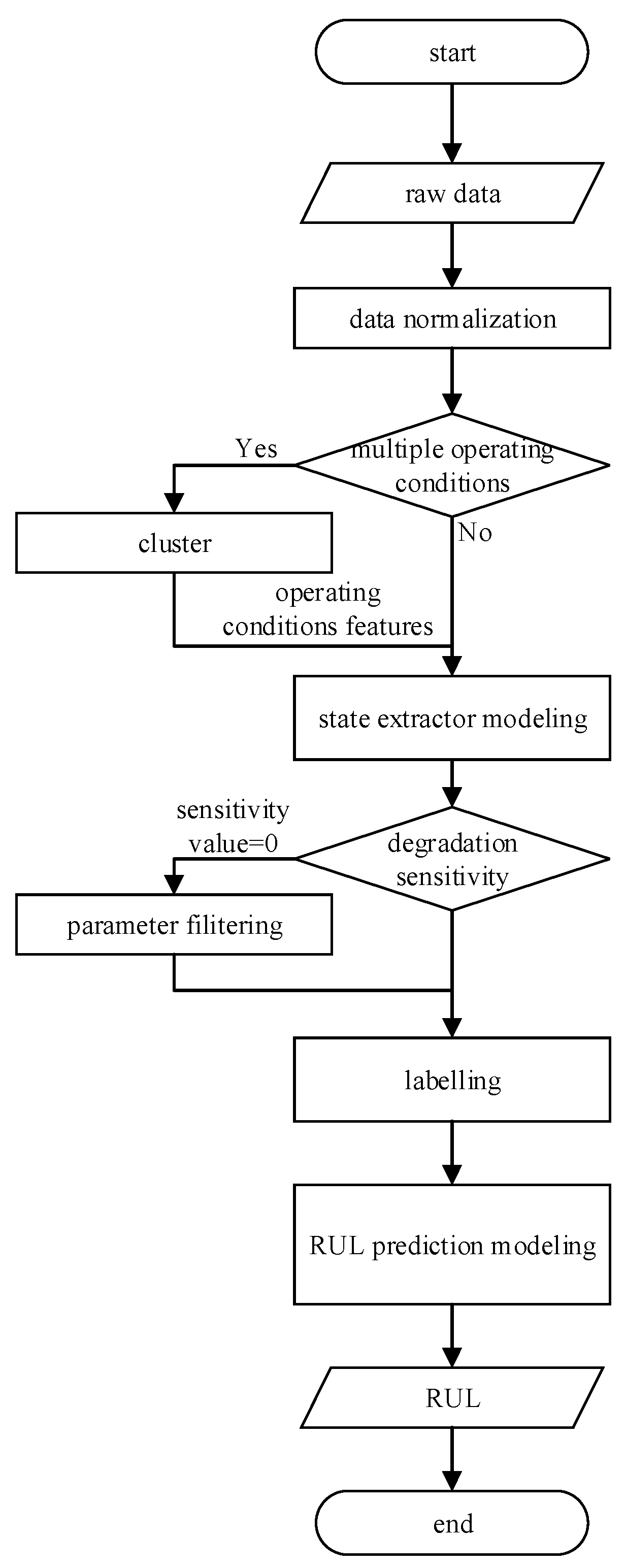
To further improve the overall application efficiency, a novel process of the RUL prediction is introduced. A state detector is built for automatic data filtering and labelling. Besides, for multiple operating conditions, new features are extracted and added by clustering. The diagram of the complete RUL estimation algorithm is displayed in Figure 5.
First, with the z-score function, data preprocessing is applied to normalize the data into 0–1. To extract the features of operating conditions, parameters are clustered with the K-means++ algorithm. Then, a state detector is built with several data points before and after the whole life. With the state detector, the first data predicted as a failure is taken as the degenerate initial point to label the RUL. Moreover, through the interpretative analysis of the modeling process, the degradation sensitivity of each parameter is obtained. The parameters with low sensitivity are removed. Finally, the efficient neural network proposed is built to achieve the learning of the RUL prediction.
3. Experiments
To assess the proposed algorithm, an experiment was carried out on the CMAPSS datasets. The outcome was compared with the vanilla LSTM and one-dimensional CNN respectively. In addition, the experiment was conducted on a fairly powerful machine: a Lenovo Workstation P520 with 32 GB of RAM and NVIDIA RTX 2080Ti GPU.
3.1. Dataset Description
The CMAPSS datasets are widely used turbofan engine degradation datasets [27,28]. As a simulation engine model of the 90,000 lb. thrust class, it includes an atmospheric model capable of simulating different altitudes, Mach numbers and temperatures for engine experimental research [29].
The CMAPSS datasets contain four sub-datasets named FD001–FD004. Each sub-dataset has 26 fields, representing the engine ID, running cycles, three operating conditions (altitude, Mach number and throttle resolver) and 21 sensor readings. The FD002 and FD004 sub-datasets have six operating modes, which can be determined by operating setting columns. However, the range of operating settings is not specified in the datasets. The running cycles of the engines from normal to damaged are recorded as life cycle. Every engine has a varied beginning wear level and manufacturing variation. Hence, for FD001, maximum life cycle means the longest running cycle of the 100 engines. Due to the different operation conditions and fault modes between four sub-datasets (FD001–FD004), the maximum life cycle varies greatly. The description of the CMAPSS datasets is shown in Table 1.
3.2. Data Pre-Processing
Consider the parameters in the CMAPSS datasets have different units and orders of magnitude. Data normalization was used to scale the data into a same specific interval. In the experiment, the sensor data was normalized by standardization (Formula (7)).
where is the original data, is the normalized result and and are mean and variance of , respectively.
Figure 6 is the data visualization for engine 1 in FD001 and FD002. There are three trends as shown, constant, ascending and descending trend, such as s1, s2, s7. All these features of FD001 are summarized in Table 2. The same characteristic was also found in FD003. However, no discernible trends of sensor readings could be found in FD002 and FD004. This may be caused by the multiple operation conditions. Hence, K-means++ was used to cluster the different operation conditions. The clustering results are displayed in Figure 7.
As shown in Figure 7, through the K-means++ algorithm, the multiple operating conditions were clustered into six clusters. The parameters varied greatly under different operation modes. It was necessary to encode these operating conditions into the input features for prediction. Hence, one hot encoding was applied to label the operation condition of the current cycle. In addition, the operating mode of each engine will change throughout its life. An extra cumulating state was also added since the start of the records for each engine. The final feature used for FD002 and FD004 is described in Figure 8; there are 36 columns of input features.
3.3. Data Cleaning and Labelling
According to Heimes’ theory, for an aero-engine history, the first 30 cycles stand for health and the final 30 cycles for degradation. Based on this assumption, ExtraTreesClassifier was applied as the state detector to identify the first sign of failure. This process can not only help to label the data, but also filter these features through the interpretive analysis of the tree model.
The first 30 healthy cycles for each engine were denoted as 0, and the final 30 degraded cycles were 1. Then, ExtraTreesClassifier was trained as a state detector. Taking engine 1 in FD001 as an example, as shown in Figure 9, the whole life of the engine was 192. The failure began to manifest at the 149 cycle. Then, the state of the engine 1 fluctuated frequently until about the 159 cycle and finally degraded. The result also confirms the effectiveness of Heimes’ assumption.
Due to the lack of a physical degradation model, it is difficult to determine the expected RUL corresponding to the running cycle. This is especially true for a complex aero-engine system. According to Heimes’ assumption, a new engine performs normally in the early stage. When the initial failure occurs, the system will linearly deteriorate. Based on the above theory, the RUL could be labelled with a piecewise linear function. The state detector determines the different engine life stages. For the early healthy state, it is labelled by the real RUL; for the fault state, it is regarded as linearly decrement with the slope of −1. Hence, for engine 1 in FD001, the visualization result of the RUL is shown in Figure 10.
In addition, by calculating the cumulative reduction of Gini coefficient of the ExtraTreesClassifier, the degradation sensitivity of 21 sensors could be obtained. As shown in Figure 11, the y axis represents the value of degradation sensitivity of different parameters. The more sensitive, the greater the value. There were six parameters that were zero. The reason is that these six parameters are constant throughout the whole life cycle in FD001, as shown in Table 2. These insensitive features not only can not improve the prediction accuracy of the algorithm, but also increase the need for computation and training time. Hence, the irrelevant parameters were deleted from the raw datasets. As shown in Figure 11a, s1, s5, s10, s16, s18 and s19 were deleted in FD001. In FD003, s1, s5, s16, s18 and s19 were deleted.
3.4. Model Configuration and Training
In the experiment, the model adopts a standard CAE and TCN structure. CAE is mainly composed of convolution block and up sampling block. Each convolution block was stacked by convolution, batch normalization, average pooling and activation function. The upsampling block is composed of transposed convolution, normalization and activation function. The encoder realizes dimension reduction through the pooling layer, and the decoder realizes dimension increase through transposed convolution. The details of CAE are shown in Table 3.
TCN is mainly composed of temporal block. Each temporal block is stacked by dilated causal convolution, weight norm, activation and dropout. In addition, skip connection is used to learn better. The details of TCN are shown in Table 4.
During the training process, the batch size was 256, Mean Square Error (MSE) and Adam were used as the loss function and optimizer. The initial learning rate was 0.01, and decayed the learning rate of each parameter group by 0.9 every 30 epochs.
3.5. Performance Evaluation
The performance of the proposed RUL estimation algorithm was evaluated with the efficiency and the accuracy. The efficiency was quantified by the training duration of the algorithm, while the accuracy was assessed by official scoring function on the CMAPSS datasets.
The scoring function is defined as follows (Formula (8), Formula (9)):
where n represents the sample size and measures the discrepancy between the estimated RUL and real RUL.
Considering that even minor delays may result in catastrophic aviation accidents, delayed forecasting is more punished than early forecasting. Besides, in order to conduct a unified comparison of different sample sizes in the four sub-datasets, the sum is replaced by the mean value.
4. Results and Discussion
The prediction performance of the proposed RUL estimation algorithm is evaluated here. It is also compared with other widely used methods, vanilla LSTM and one-dimensional CNN.
4.1. Prediction Performance
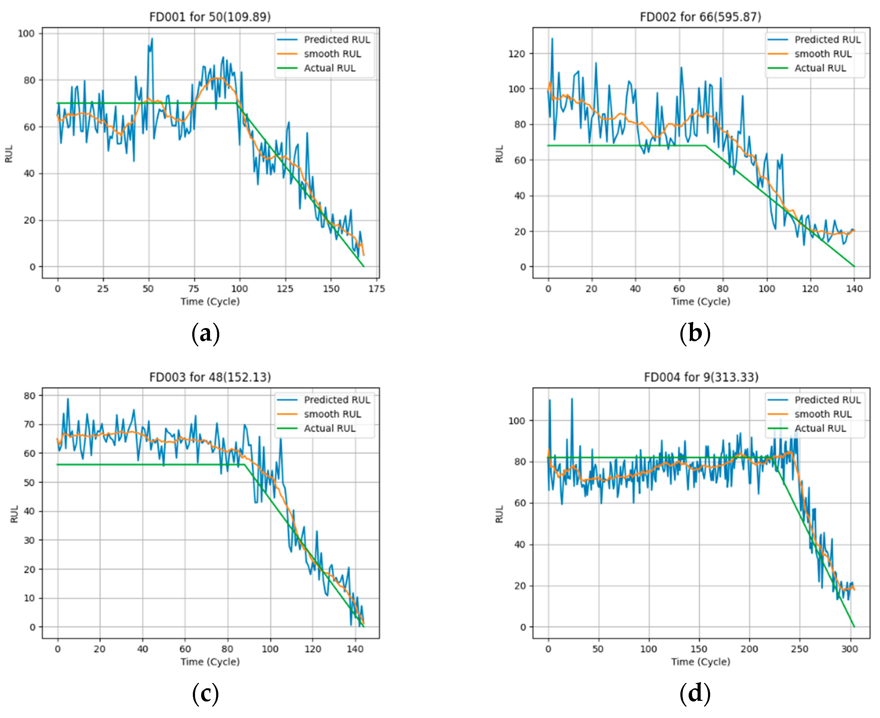
To observe the prediction effect of the proposed algorithm, four engines wer randomly selected from FD001 to FD004, respectively. The RUL of the whole running cycle was predicted, and the outcomes were smoothed by the exponential smoothing. The final results of these four engines are shown in Figure 12. It can be seen that the proposed algorithm can meet the expectations to realize the prediction of the RUL.
In order to further analyze the prediction effect of the proposed algorithm, the good, bad and average estimation results in FD001 were selected for visualization, as shown in Figure 13.
As shown in the Figure 13, a good result basically matches the real RUL curve. The poor and average results can also be well predicted in the degradation stage. The main differences between good, poor and average is the prediction of health stage. The main reason is the labeling of the RUL, the transition from health stage to degradation stage is too sudden. Therefore, a more reasonable annotation method should be improved in the future research.
4.2. Comparison
The efficiency and accuracy of the proposed algorithm are compared with other commonly used models, one-dimensional CNN and vanilla LSTM. For the one-dimensional CNN, the same architecture as TCN is used. For vanilla LSTM, generally two to three layers can achieve better learning. Therefore, three layers of LSTM are used. For each layer, the number of neurons is equal to the maximum number of one-dimensional CNN kernel. In addition, the training strategies of the three models are exactly the same. The comparison results are as shown in Table 5 and Table 6.
As shown in Table 5 and Table 6, the proposed algorithm shows great advantages in efficiency and accuracy. It has the shortest training duration and the lowest official score.
Since the model structure is mainly based on one-dimensional CNN layer, the proposed algorithm has no obvious advantages over one-dimensional CNN in training duration. In contrast, LSTM needs to iterate on the time dimension, and cannot be implemented in parallel like convolution. Therefore, there is a significant gap between the training duration of the proposed model and the vanilla LSTM on FD001 to FD004. In other words, the algorithm proposed has a higher application efficiency.
In terms of precision comparison, the official scores of the proposed algorithm on the four sub-datasets are smallest. This implies better predictive power. By comparing the results of four sub-datasets, it can be found that the algorithm achieved the best results in FD001 and the worst results in FD004. This is in line with expectations. The prediction effect is negatively correlated with the data complexity. Moreover, the algorithm proposed shows more significant advantages for FD002–FD004. The main reason is that the complexity of the four sub-datasets is different. Compared with FD001, the data from FD002–FD004 is more complex, more operation conditions or more fault modes. Hence, with the same parameters, the RUL prediction model needs to be able to learn the deeper information in the data. For the proposed algorithms, CAE was used to learn the degradation trend. This can reduce the dimension of the data. The key information of degradation was extracted, as well as the noise reduction. To learn the degradation trend and realize time series prediction, TCN was used. Compared with the traditional one-dimensional CNN, TCN is a one-way structure with time constraints. Therefore, TCN is more sensitive to changes in time dimension. LSTM memorizes time information through iteration in time. When the time is longer or the information to be learned is more complex, LSTM is prone to the problem of gradient vanishing. TCN can realize information learning of long time series through the size of dilation and kernels. Meanwhile, it adds skip connection to prevent gradient problems. Therefore, from the perspective of model structure, the proposed model has better learning ability in the face of complex time series information. In summary, as the data situation becomes more complex, the advantages of the proposed model become more obvious. In a word, the proposed algorithm has better robustness in the RUL prediction under complex conditions.
5. Conclusions
In this paper, in order to achieve an efficient and accurate RUL prediction of the aero-engine, a novel RUL estimation algorithm is proposed. Firstly, a more efficient RUL prediction model is introduced. By replacing LSTM with CNN, the model can realize more efficient learning and prediction, while ensuring the ability of temporal features extraction. It is mainly composed of convolution, it can realize parallel training through multiple GPUs in practical engineering, so as to realize real-time life prediction through faster training. This advantage can also be found in the process of training and prediction. By comparison on the CMAPSS datasets, the proposed algorithm shows high efficiency in training duration, and has better temporal feature extraction ability than one-dimensional CNN and vanilla LSTM. Besides, in case of multiple operating conditions and fault modes, the algorithm proposed has stronger robustness. Secondly, the data preprocessing process is improved in the algorithm. ExtraTreesClassifier is used as a state extractor to realize the identification of state and the degradation sensitivity analysis of parameters. This process helps achieve dimension reduction and the RUL annotation which could be applied in practical engineering. It is of great significance for the automation of the RUL prediction and further improving the efficiency and accuracy of the algorithm.
Author Contributions
Main ideas and overall framework of the paper, G.R.; Main experiment, Y.W.; Paper algorithm guidance, Z.S.; Experimental guidance, G.Z.; Experimental validation, F.J.; Original draft review, J.W. All authors have read and agreed to the published version of the manuscript.
Funding
The work is supported by BJNSF (L191021) and National Science and Technology Major Project (2017-I-0006- 0007).
Institutional Review Board Statement
Not applicable.
Informed Consent Statement
Not applicable.
Acknowledgments
This paper is an extended version of the paper “Aero-Engine Remaining Useful Life Estimation based on 1-Dimensional FCN-LSTM Neural Networks”, published at the 38th Chinese Control Conference, Guangzhou, China, 4913-4918 July 2019. In addition, I appreciate NASA Ames Research Center for providing the turbofan engine degradation simulation dataset.
Conflicts of Interest
The authors declare no conflict of interest. The funders had no role in the design of the study; in the collection, analyses, or interpretation of data; in the writing of the manuscript; or in the decision to publish the results.
References
- Li, X.; Ding, Q.; Sun, J.Q. Remaining useful life estimation in prognostics using deep convolution neural networks. Reliabil. Eng. Syst. Saf. 2018, 172, 1–11. [Google Scholar] [CrossRef] [Green Version]
- Azadeh, A.; Asadzadeh, S.M.; Salehi, N.; Firoozi, M. Condition-based maintenance effectiveness for series-parallel power generation system—A combined Markovian simulation model. Reliabil. Eng. Syst. Saf. 2015, 142, 357–368. [Google Scholar] [CrossRef]
- Zaidan, M.A.; Mills, A.R.; Harrision, R.F. Bayesian framework for aerospace gas turbine engine prognostics. In Proceedings of the 2013 IEEE Aerospace Conference, Big Sky, MT, USA, 2–9 March 2013; pp. 1–8. [Google Scholar]
- Qian, Y.; Yan, R.; Gao, R.X. A multi-time scale approach to remaining useful life prediction in rolling bearing. Mech. Syst. Signal. Process. 2017, 83, 549–567. [Google Scholar] [CrossRef] [Green Version]
- Jouin, M.; Gouriveau, R.; Hissel, D.; Pra, M.-C.; Zerhouni, N. Particle filter-based prognostics: Review, discussion and perspectives. Mech. Syst. Signal. Process. 2016, 7273, 2–31. [Google Scholar] [CrossRef]
- Jouin, M.; Gouriveau, R.; Hissel, D.; Pra, M.-C.; Zerhouni, N. Degradations analysis and aging modeling for health assessment and prognostics of PEMFC. Reliabil. Eng. Syst. Saf. 2016, 148, 78–95. [Google Scholar] [CrossRef]
- Ali, J.B.; Chebel-Morello, B.; Saidi, L.; Malinowski, S.; Fnaiech, F. Accurate bearing remaining useful life prediction based on Weibull distribution and artificial neural network. Mech. Syst. Signal. Process. 2015, 5657, 150–172. [Google Scholar]
- Jun, Z.; Nan, C.; Weiwen, P. Estimation of bearing remaining useful life based on multiscale convolutional neural network. IEEE Trans. Ind. Electron. 2018, 66, 3208–3216. [Google Scholar]
- Li, Y.; Shi, J.; Wang, G.; Liu, X. A data-driven prognostics approach for RUL based on principle component and instance learning. In Proceedings of the IEEE International Conference on Prognostics and Health Management (ICPHM), Ottawa, ON, Canada, 20–22 June 2016; pp. 1–7. [Google Scholar]
- Khelif, R.; Chebel-Morello, B.; Malinowski, S.; Laajili, E.; Fnaiech, F.; Zerhouni, N. Direct remaining useful life estimation based on support vector regression. IEEE Trans. Ind. Electron. 2017, 64, 2276–2285. [Google Scholar] [CrossRef]
- Dong, M.; He, D. A segmental hidden semi-Markov model (HSMM)-based diagnostics and prognostics framework and methodology. Mech. Syst. Signal. Process. 2007, 21, 2248–2266. [Google Scholar] [CrossRef]
- Peel, L. Data driven prognostics using a Kalman filter ensemble of neural network models. In Proceedings of the 2008 International Conference on Prognostics and Health Management, Denver, CO, USA, 6–9 October 2008. [Google Scholar]
- Zhang, C.; Lim, P. Multi-objective deep belief networks ensemble for remaining useful life estimation in prognostics. IEEE Trans. Neural. Netw. Learn Syst. 2017, 28, 2306–2318. [Google Scholar] [CrossRef] [PubMed]
- Babu, G.S.; Zhao, P.; Li, X.L. Deep convolutional neural network based regression approach for estimation of remaining useful life. In Proceedings of the International Conference on Database Systems for Advanced Applications, Dallas, TX, USA, 16–19 April 2016; pp. 214–228. [Google Scholar]
- Heimes, F.O. Recurrent neural networks for remaining useful life estimation. In Proceedings of the International Conference on Prognostics and Health Management, Denver, CO, USA, 6–9 October 2008. [Google Scholar]
- Wu, Y.; Yuan, M.; Dong, S.; Lin, L.; Lin, Y. Remaining useful life estimation of engineered systems using vanilla LSTM neural networks. Neurocomputing 2017, 275, 167–179. [Google Scholar] [CrossRef]
- Ince, T.; Kiranyaz, S.; Eren, L.; Askar, M.; Gabbouj, M. Real-time motor fault detection by 1-D convolutional neural network. IEEE Trans. Ind. Electron. 2016, 63, 7067–7075. [Google Scholar] [CrossRef]
- Ackley, D.H.; Hinton, G.E.; Sejnowski, T.J. A learning algorithm for Boltzmann machines. Cogn. Sci. 1985, 9, 147–169. [Google Scholar] [CrossRef]
- Hinton, G.E. Connectionist learning procedures. In Machine Learning; Morgan Kaufmann: Burlington, MA, USA, 1990; pp. 555–610. [Google Scholar]
- LeCun, Y. Modèles connexionnistes de l’apprentissage. Ph.D. Thesis, Universite P. et M. Curie, Paris, France, 1987. [Google Scholar]
- Bourlard, H.; Kamp, Y. Auto-association by multilayer perceptrons and singular value decomposition. Biol. Cybern. 1988, 59, 291–294. [Google Scholar] [CrossRef] [PubMed]
- Goodfellow, I.; Bengio, Y.; Courville, A. Deep Learning; MIT Press: Cambridge, MA, USA, 2016. [Google Scholar]
- Kiranyaz, S.; Ince, T.; Gabbouj, M. Real-time patient-specific ECG classification by 1-D convolutional neural networks. IEEE Trans. Biomed. Eng. 2016, 63, 664–675. [Google Scholar] [CrossRef] [PubMed]
- Kim, S.; Choi, J. Convolutional neural network for gear fault diagnosis based on signal segmentation approach. Struct. Health Monit. 2019, 18, 1401–1415. [Google Scholar] [CrossRef]
- Sun, W.; Shao, S.; Zhao, R.; Yan, R.; Zhang, X.; Chen, X. A sparse auto-encoder-based deep neural network approach for induction motor faults classification. Measurement 2016, 89, 171–178. [Google Scholar] [CrossRef]
- van den, O.A.; Dieleman, S.; Zen, H.; Simonyan, K.; Vinyals, O.; Graves, A.; Kalchbrenner, N.; Senior, A.W.; Kavukcuoglu, K. “WaveNet: A Generative Model for Raw Audio. arXiv 2016, arXiv:1609.03499. [Google Scholar]
- Saxena, A.; Goebel, K. Turbofan Engine Degradation Simulation Data Set; NASA Ames: Mountain View, CA, USA, 2008. [Google Scholar]
- Prognostics Data Repository; NASA Ames Research Center: Moffett Field, CA, USA, 2008.
- Saxena, A.; Goebel, K.; Simon, D.; Eklund, N. Damage propagation modeling for aircraft engine run-to-failure simulation. In Proceedings of the International Conference on Prognostics and Health Management, Denver, CO, USA, 6–9 October 2008. [Google Scholar]
Figure 1.
Autoencoder.

Figure 2.
One-dimensional CNN.

Figure 3.
TCN.

Figure 4.
The RUL estimation model structure.

Figure 5.
Diagram of the RUL estimation algorithm.

Figure 6.
(a) Normalized sensor data of engine 1 in FD001; (b) Normalized s1, s2 and s7 of engine 1 in FD001; (c) Normalized sensor data of engine 1 in FD002; (d) Normalized s1, s2 and s7 of engine 1 in FD002. (Different colors represent different sensor data in subfigures a and c.)
Figure 6.
(a) Normalized sensor data of engine 1 in FD001; (b) Normalized s1, s2 and s7 of engine 1 in FD001; (c) Normalized sensor data of engine 1 in FD002; (d) Normalized s1, s2 and s7 of engine 1 in FD002. (Different colors represent different sensor data in subfigures a and c.)

Figure 7.
Operation setting clusters on FD002. (Different triangles represent a specific operating condition.)
Figure 7.
Operation setting clusters on FD002. (Different triangles represent a specific operating condition.)

Figure 8.
Final input features of FD002 and FD004.

Figure 9.
State detection of engine 1 in FD001.

Figure 10.
The RUL of engine 1 in FD001.

Figure 11.
(a) Degradation sensitivity of sensors in FD001; (b) Degradation sensitivity of sensors in FD003.
Figure 11.
(a) Degradation sensitivity of sensors in FD001; (b) Degradation sensitivity of sensors in FD003.

Figure 12.
(a) Prediction performance of engine 50 in FD001; (b) Prediction performance of engine 66 in FD002; (c) Prediction performance of engine 48 in FD003; (d) Prediction performance of engine 9 in FD004.
Figure 12.
(a) Prediction performance of engine 50 in FD001; (b) Prediction performance of engine 66 in FD002; (c) Prediction performance of engine 48 in FD003; (d) Prediction performance of engine 9 in FD004.

Figure 13.
(a) Good result for FD001; (b) Poor result for FD001; (c) Average result for FD001.


Table 1.
Description of the CMAPSS datasets.
| Dataset | CMAPSS | ||||
|---|---|---|---|---|---|
| FD001 | FD002 | FD003 | FD004 | ||
| Training dataset | Engine units | 100 | 260 | 100 | 249 |
| Total samples | 20,631 | 53,759 | 24,720 | 61,249 | |
| Maximum life cycles | 362 | 378 | 525 | 543 | |
| Minimum life cycles | 128 | 128 | 145 | 128 | |
| Testing dataset | Engine units | 100 | 259 | 100 | 248 |
| Maximum cycles | 303 | 367 | 475 | 486 | |
| Minimum cycles | 31 | 21 | 38 | 19 | |
| Total samples | 13,096 | 33,991 | 16,596 | 41,214 | |
| Operating conditions | 1 | 6 | 1 | 6 | |
| Fault modes | 1 | 1 | 2 | 2 | |
Table 2.
Sensor data trends of FD001.
| Trend | Sensor NO. |
|---|---|
| Ascending | 2, 3, 4, 8, 11, 13, 15, 17 |
| Descending | 7, 9, 12, 14, 20, 21 |
| Constant | 1, 5, 10, 16, 18, 19 |
Table 3.
CAE model structure.
| Name | (Kernel, Stride, Padding) | |
|---|---|---|
| 1 | Convolution block | (3, 1, 1), (2, 2) |
| 2 | Convolution block | (3, 1, 1), (2, 2) |
| 3 | Convolution block | (3, 1, 1), (2, 2) |
| 4 | Convolution layer | (2, 1) |
| 5 | Upsampling block | (4, 2, 1) |
| 6 | Upsampling block | (4, 2, 1) |
| 7 | Upsampling block | (3, 2) |
| 8 | Upsampling block | (4, 2, 1) |
Table 4.
TCN model structure.
| Name | (Kernel, Stride, Dilation) | |
|---|---|---|
| 1 | Temporal block | (3, 1, 1) |
| 2 | Temporal block | (3, 1, 2) |
| 3 | Temporal block | (3, 1, 4) |
| 4 | Linear layer | / |
Table 5.
Efficiency comparison of training duration on the CMAPSS datasets.
| FD001 | FD002 | FD003 | FD004 | |
|---|---|---|---|---|
| Proposed network | 0.26 s | 0.80 s | 0.31 s | 0.93 s |
| One-Dimensional CNN | 0.28s | 1.06s | 0.34s | 1.24s |
| LSTM | 0.62s | 1.64s | 0.75s | 1.95s |
Table 6.
Performance comparisons of the score on the CMAPSS datasets.
| Test score | FD001 | FD002 | FD003 | FD004 |
|---|---|---|---|---|
| Proposed network | 3.72 | 26.57 | 7.36 | 56.75 |
| One-Dimensional CNN | 7.22 | 67.32 | 11.04 | 80.24 |
| LSTM | 5.27 | 50.81 | 9.84 | 73.18 |
Disclaimer/Publisher’s Note: The statements, opinions and data contained in all publications are solely those of the individual author(s) and contributor(s) and not of MDPI and/or the editor(s). MDPI and/or the editor(s) disclaim responsibility for any injury to people or property resulting from any ideas, methods, instructions or products referred to in the content. |
© 2022 by the authors. Licensee MDPI, Basel, Switzerland. This article is an open access article distributed under the terms and conditions of the Creative Commons Attribution (CC BY) license (https://creativecommons.org/licenses/by/4.0/).
Share and Cite
MDPI and ACS Style
Ren, G.; Wang, Y.; Shi, Z.; Zhang, G.; Jin, F.; Wang, J. Aero-Engine Remaining Useful Life Estimation Based on CAE-TCN Neural Networks. Appl. Sci. 2023, 13, 17. https://0-doi-org.brum.beds.ac.uk/10.3390/app13010017
AMA Style
Ren G, Wang Y, Shi Z, Zhang G, Jin F, Wang J. Aero-Engine Remaining Useful Life Estimation Based on CAE-TCN Neural Networks. Applied Sciences. 2023; 13(1):17. https://0-doi-org.brum.beds.ac.uk/10.3390/app13010017
Chicago/Turabian StyleRen, Guanghao, Yun Wang, Zhenyun Shi, Guigang Zhang, Feng Jin, and Jian Wang. 2023. "Aero-Engine Remaining Useful Life Estimation Based on CAE-TCN Neural Networks" Applied Sciences 13, no. 1: 17. https://0-doi-org.brum.beds.ac.uk/10.3390/app13010017
Note that from the first issue of 2016, this journal uses article numbers instead of page numbers. See further details here.