A Novel Rolling Bearing Fault Diagnosis Method Based on MFO-Optimized VMD and DE-OSELM

Abstract

Rolling bearings are critical in maintaining smooth operation of rotating machinery and considerably influence its reliability. The signals collected from rolling bearings in field conditions are often subjected to noise, creating a challenge to extract weaker fault features. This paper proposes a rolling bearing fault diagnosis method that addresses the above-mentioned problem through the moth-flame optimization algorithm optimized variational mode decomposition (MFO-optimized VMD) and an ensemble differential evolution online sequential extreme learning machine (DE-OSELM). By using the dynamic adaptive weight factor and genetic algorithm cross operator, the optimization accuracy and global optimization ability of the moth-flame optimization (MFO) are improved, and the two basic parameters of VMD decomposition level and quadratic penalty factor are adaptive selected. Since the vibration characteristics of the signal cannot be fully interpreted by a single index, The effective weighted correlation sparsity index (EWCS) is utilized to extract the relevant intrinsic mode functions (IMF) of VMD decomposition and extract their energies as features. In order to improve the classification accuracy, The energy feature set is subsequently inputted into DE-OSELM for training and classification purposes, and the proposed method is assessed via a sample set with four different health states of actual rolling bearings. Our proposed method results are compared with other diagnosis methods, proving its feasibility to diagnose rolling bearing faults with higher classification accuracy.

1. Introduction

Rolling bearings are one of the most widely used mechanical components in rotary machinery and have diverse applications in the medical, aerospace, and railway fields [1,2,3]. Bearing failures account for 30% of rotating machinery failures, according to published research [4]. Ensuring the normal and safe operation of rolling bearings thus demands state monitoring and fault diagnosis [5]. When a rolling bearing fails, vibration signals emit regular pulse signals, which analysts often scrutinize to identify the specific type of failure [6,7,8]. However, the noisy nature of collected vibration signals poses difficulties in extracting fault features from pulse signals, which is an area of active research in the field of fault diagnosis.

Several approaches have been proposed for processing vibration signals, including empirical mode decomposition (EMD) [9,10,11], ensemble empirical mode decomposition (EEMD) [12,13,14], and the local mean decomposition method (LMD) [15,16,17]. Nonetheless, modal-analysis-based approaches, such as EMD, EEMD, and LMD, are limited in that they cannot fully address the issue of modal mixing and endpoint effect. Dragomiretskity et al. [18] introduced an adaptive signal analysis approach named VMD that deals with signal processing by formulating and resolving variational issues, providing strong resistance to noise. Owing to its ability to tackle modal mixing and endpoint effect effectively, VMD finds applications in multiple fields, including generator anomaly detection, structural health monitoring, and bearing fault diagnosis [19,20,21]. Li and colleagues [22] devised a diagnosis method for fault detection in rolling bearings using VMD and improved Kernel Extreme Learning Machine and demonstrated that VMD successfully addressed the mode mixing problem and boasted superior computational efficiency compared to EMD and LMD methods.

However, VMD requires pre-set parameters, including the decomposition number (K) and penalty factor (α), which significantly affect the final outcome. To identify the optimal parameter combination, several studies have proposed different methods. For instance, Jiang et al. [19] established a central frequency mode decomposition (CFMD), based on VMD, and the difficulty of the selection of initial parameters in the traditional VMD was relieved, provided that the range of bandwidth parameters was preset. Wang et al. [23] compared the center frequency of modal components that were decomposed by different parameter combinations. However, this method had limited adaptability. Tang et al. [24] implemented the Particle Swarm Optimization (PSO) algorithm to optimize VMD and demonstrated its ability to extract early fault features from bearing vibrations. Another study by Zhang et al. [25] suggested a parameter adaptive VMD strategy based on the grasshopper optimization algorithm (GOA) and validated its efficiency in analyzing the vibration signals of real rotating machinery. Moreover, Gu et al. [26] adopted the grey wolf optimizer (GWO) algorithm, which was superior to the fixed-parameter VMD and maximum weighted kurtosis optimization VMD in terms of selecting the optimal parameter combination. These studies show that optimization algorithms with strong search abilities can achieve better adaptive selection of VMD parameters. Recently, the MFO algorithm [27] has achieved excellent performance in solving engineering optimization problems [28,29]. Sivalingam et al. [30] compared MFO with other optimization algorithms, finding that MFO performed the best. However, the original MFO algorithm searches in the region around its unique flame, hence increasing the risk of falling into the local optimum and slow convergence speed. Therefore, the original MFO algorithm requires improvement. Although VMD can effectively solve the modal problem, there will still be false intrinsic modal functions (IMF) in the decomposed IMF, which will affect the accuracy of the fault classification of rolling bearings [31]. Therefore, it is necessary to screen the decomposed IMF.

In addition to feature extraction, the swift and accurate identification of fault types is pivotal for fault diagnosis. ELM replaces the gradient descent algorithm with a random assignment method and enhances the generalization ability of traditional classification networks, making it effective for fault diagnosis [32]. Jiang et al. [33] proposed a fault diagnosis model based on multiscale weighted permutation entropy (MWPE) and ELM, which demonstrated superior recognition accuracy and speed compared to using various multiscale feature extraction methods with BPNNs and SVMs. Similarly, Lan et al. [34] achieved the diagnosis of slipper abrasion faults using ELM and demonstrated that the classification performance of ELM is superior to BP and SVM. Liang et al. [35] proposed OSELM to resolve the long training time issue of ELM when the training data were large. This algorithm obviates the need to retrain historical data to facilitate rapid diagnosis. Sahani et al.’s use of VMD and OSELM for real-time detection and classification of power quality events provided high classification accuracy and robustness [36]. However, the randomly generated input weight and hidden layer bias in the OSELM algorithm have been found to limit its prediction accuracy and robustness. Hence, this paper introduces the ensemble DE-OSELM method, which was proposed by Zhou et al. [37], to realize fault classification and diagnosis.

This paper presents a novel approach for detecting rolling bearings faults, utilizing optimized VMD and DE-OSELM. Firstly, the method adopts a dynamic adaptive weight factor and a crossover operator. Compared with the original MFO algorithm and other intelligent optimization algorithms, the improved MFO algorithm has higher global optimization ability and search accuracy, and it solves the problem of sub-optimal performance and limited convergence accuracy of multi-objective optimization algorithm. Secondly, the improved MFO is used to optimize VMD and overcome the susceptibility of VMD parameters to artificial settings, thus facilitating the adaptive selection of these parameters. Thirdly, since the vibration characteristics of the signal cannot be fully interpreted by a single index, this method introduces a new evaluation index, the effective weighted correlation sparsity index, to strip false modal components and filter the IMF recovered through VMD decomposition. The energy features of the effective IMFs are subsequently extracted as feature vectors. Finally, in order to improve the classification accuracy, the energy eigenmatrix is normalized and subjected to DE-OSELM training to identify the fault type.

2. Basic Principle

VMD is an adaptive signal processing technique that relies on the formulation and resolution of variational problems [38]. Essentially, the VMD algorithm partitions the input signal into $K$ IMFs while simultaneously minimizing the estimated broadband sum. To achieve this, the algorithm operates under the assumption that the sum of the IMF components is equivalent to that of the original signal. The corresponding variational problem is subject to certain constraints and can be expressed as:

$$\{\begin{array}{l}{\min }_{\{{u_k\}}_{,}\{{\omega }_k\}}\{{\displaystyle {\sum }_k{\Vert {\partial }_t[(\delta (t)+\frac{j}{\pi t})\ast u_k(t)]e^{-j{\omega }_{k}t}\Vert }_2^2}\}\\ s.t.{\displaystyle {\sum }_k{u}_k=f}\end{array}$$

(1)

where; $u_k$ is the decomposed IMF components, and ${\omega }_k$ is the central frequency of each IMF component.

The problem is solved by introducing a penalty factor $\alpha$ and a Lagrange multiplier operator $\lambda$ into the model, thereby transforming it into an unconstrained variational problem.

$$L(u_k,{\omega }_k,\lambda )=\alpha {{\displaystyle {\sum }_k\Vert {\partial }_t[(\delta (t)+\frac{j}{\pi t})\ast u_k(t)]e^{-j{\omega }_{k}t}\Vert }}_2^2+{\Vert f-{\displaystyle {\sum }_k{u}_k}\Vert }_2^2+\langle \lambda ,f-{\displaystyle {\sum }_k{u}_k}\rangle$$

(2)

where; $f$ is the original signal.

The steps for solving Equation (2) are as follows:

Initialize parameters $\left\{{\widehat{u}}_k^1\right\}$, $\left\{{\widehat{\omega }}_k^1\right\}$, $\left\{{\widehat{\lambda }}^1\right\}$, and set $n=0$;

Let $n\to n+1$, an update $u_k$, ${\omega }_k$, $\lambda$ iteratively according to Equations (3)–(5):

$${\widehat{u}}_k^{n+1}(\omega )=\frac{\widehat{f}(\omega )-{\displaystyle {\sum }_{i\ne k}{\widehat{u}}_i(\omega )+\frac{\widehat{\lambda }(\omega )}{2}}}{1+2\alpha {(\omega -{\omega }_k)}^2}$$

(3)

$${\omega }_k^{n+1}=\frac{{\displaystyle {\int }_0^{\infty }\omega {\left|{\widehat{u}}_k(\omega )\right|}^{2}d\omega }}{{\displaystyle {\int }_0^{\infty }{\left|{\widehat{u}}_k(\omega )\right|}^{2}d\omega }}$$

(4)

$${\widehat{\lambda }}^{n+1}(\omega )={\widehat{\lambda }}^n(\omega )+\tau (\widehat{f}(\omega )-{\displaystyle {\sum }_{k=1}^k{\widehat{u}}_k^{n+1}(\omega )})$$

(5)

where; $n$ is the number of iterations, $\wedge$ is the Fourier transform, and $\tau$ is the noise tolerance.

Repeat Step 2 until the cycle ends, when the components satisfy Equation (6), and $K$ IMFs are obtained.

$${\displaystyle {\sum }_{k=1}^k\frac{{\Vert u_k^{n+1}-u_k^n\Vert }_2^2}{{\Vert u_k^n\Vert }_2^2}}<\epsilon$$

(6)

where; $\epsilon$ is the discriminant accuracy.

Proper parameter selection is a prerequisite for VMD signal decomposition, where the parameters $K$ and $\alpha$ exert major influence on the decomposition effect, whereas the parameters $\epsilon$ and $\tau$ play a less prominent role [39]. Hence, achieving the optimal VMD decomposition effect warrants the identification of suitable $K$ and $\alpha$ values.

3. MFO Algorithm and Its Improvement

3.1. MFO Algorithm

Inspired by the natural phenomenon of moths fighting fire, the MFO algorithm assumes that the moth population flies around the flame population in the form of a logarithmic spiral curve. If a new position is found to be better than the original flame position, the position will be updated. The matrix $M$ represents the initial moth position, and the matrix $OM$ represents the initial moth fitness value, as given below.

$$M=\left(\begin{array}{c}{M}_1\\ M_2\\ ⋮\\ M_n\end{array}\right)=\left(\begin{array}{c}{m}_{1,1}\\ m_{2,1}\\ ⋮\\ m_{n,1}\end{array}\begin{array}{c}{m}_{1,2}\\ m_{2,2}\\ ⋮\\ m_{n,2}\end{array}\begin{array}{c}\cdots \\ \cdots \\ \ddots \\ \cdots \end{array}\begin{array}{c}{m}_{1,d}\\ m_{2,d}\\ ⋮\\ m_{n,d}\end{array}\right)$$

(7)

where; $M_i$ is the position of the $i-th$ moth in the solution space of the moth population $M$; $n$ is the population number; and $d$ is the dimension of the solution space.

$$OM=\left(\begin{array}{c}O{M}_1\\ O{M}_2\\ ⋮\\ O{M}_n\end{array}\right)$$

(8)

where; $O{M}_i$ is the fitness value of the $i-th$ moth.

Each moth has a unique flame corresponding to it. The flame represents the local optimal solution found by each moth in the search process. The flame position is represented by the matrix $F$, and the matrix $OF$ represents the flame fitness value.

$$F=\left(\begin{array}{c}{F}_1\\ F_2\\ ⋮\\ F_n\end{array}\right)=\left(\begin{array}{cccc}{f}_{1,1}& f_{1,2}& \cdots & f_{1,d}\\ f_{2,1}& f_{2,2}& \cdots & f_{2,d}\\ ⋮& ⋮& \ddots & ⋮\\ f_{n,1}& f_{n,2}& \cdots & f_{n,d}\end{array}\right)$$

(9)

where; $F_i$ is the position of the $i-th$ flame in the solution space of flame population $F$; $n$ is the number of flame population; and $d$ is the dimension of solution space.

$$OF=\left(\begin{array}{c}O{F}_1\\ O{F}_2\\ ⋮\\ O{F}_n\end{array}\right)$$

(10)

where; $O{F}_i$ is the fitness value of the $i-th$ flame.

Moth $M_i$ will move towards the corresponding flame $F_j$ in the form of a logarithmic spiral curve due to phototaxis. The movement formula is defined as Equation (11), and the matrix $S(M_i,F_j)$ represents the updated position of the moth.

$$S(M_i,F_j)=D_i\cdot e^{bt}\cdot \cos (2\pi t)+F_j$$

(11)

where; $M_i$ is the $i-th$ moth; $F_j$ is the $j-th$ flame; $D_i$ is the distance between the $i-th$ moth and the $j-th$ flame; $b$ is a constant related to the shape of the spiral function; and $t$ is a random number in the interval [−1, 1].

The algorithm adaptively reduces the number of flames based on Equation (12), thereby enhancing its efficiency and ensuring that the population of moths is converging towards the optimal flame.

$$flameno=round(N-l\frac{N-1}{T})$$

(12)

where; $flameno$ is the number of current flames; $N$ is the number of original flame population; $l$ is the number of current iterations; and $T$ is the maximum number of iterations.

For the MFO algorithm, a good moth population and flame population after the initial position of the each moth are usually around the corresponding search flame area, and moths will follow the flame along into local optimum only if the flame in a local optimum. Thus, the original MFO is unable to jump out from the local optimum, which leads to the relatively low convergence accuracy and slow convergence speed.

3.2. The Improved MFO Algorithm

To address the issues related to local optimization, low convergence accuracy, and slow convergence speed of the original optimization algorithm, the MFO is modified by using both a dynamic adaptive weight factor and a crossover operator to improve the performance in terms of global optimization ability, accuracy, and efficiency.

In the original concept of the MFO algorithm, the moth population is supposed to fly around the flame population in the form of a logarithmic spiral curve, and the flame is not fully utilized, which makes the algorithm fall into local optimal easily. To improve its global optimization ability and convergence speed, the dynamic adaptive weight factor $\mu$ is introduced into the position updating strategy of moths, as formulated below.

$$\mu =\frac{1+\cos (\frac{l\pi }{T})}{2}$$

(13)

where; $l$ represents the current iteration number, and $T$ represents the maximum iteration number. The updated moth position combined with the adaptive weight factor $\mu$ is introduced in Equation (14).

$$S(M_i,F_j)=\mu \cdot D_i\cdot e^{bt}\cdot \cos (2\pi t)+\mu \cdot F_j$$

(14)

The gradual decrease as the iteration $\mu$ increases from 1 to 0 results in an enlarged search scope during the initial stages. Consequently, the algorithm performance significantly improves concerning search and global optimization abilities, accuracy, and efficiency.

In order to effectively elevate the algorithm out of local optima, the positions of the front $m$ flames are disordered by applying the crossover operator from the genetic algorithm. The main idea is to make $p$ times of cross recombination of each dimension data in the matrix involving front $m$ flames, and the corresponding dimension data of other flames are combined into a new flame. If the fitness value of the new flame is better than the original flame, the original flame will be replaced. The flame population contains a relatively high diversity and can jump out of local optimum in a certain probability by perturbation of the front $m$ optimal flames.

The process for improving the MFO is shown in Figure 1.

3.3. Verification of the Algorithm

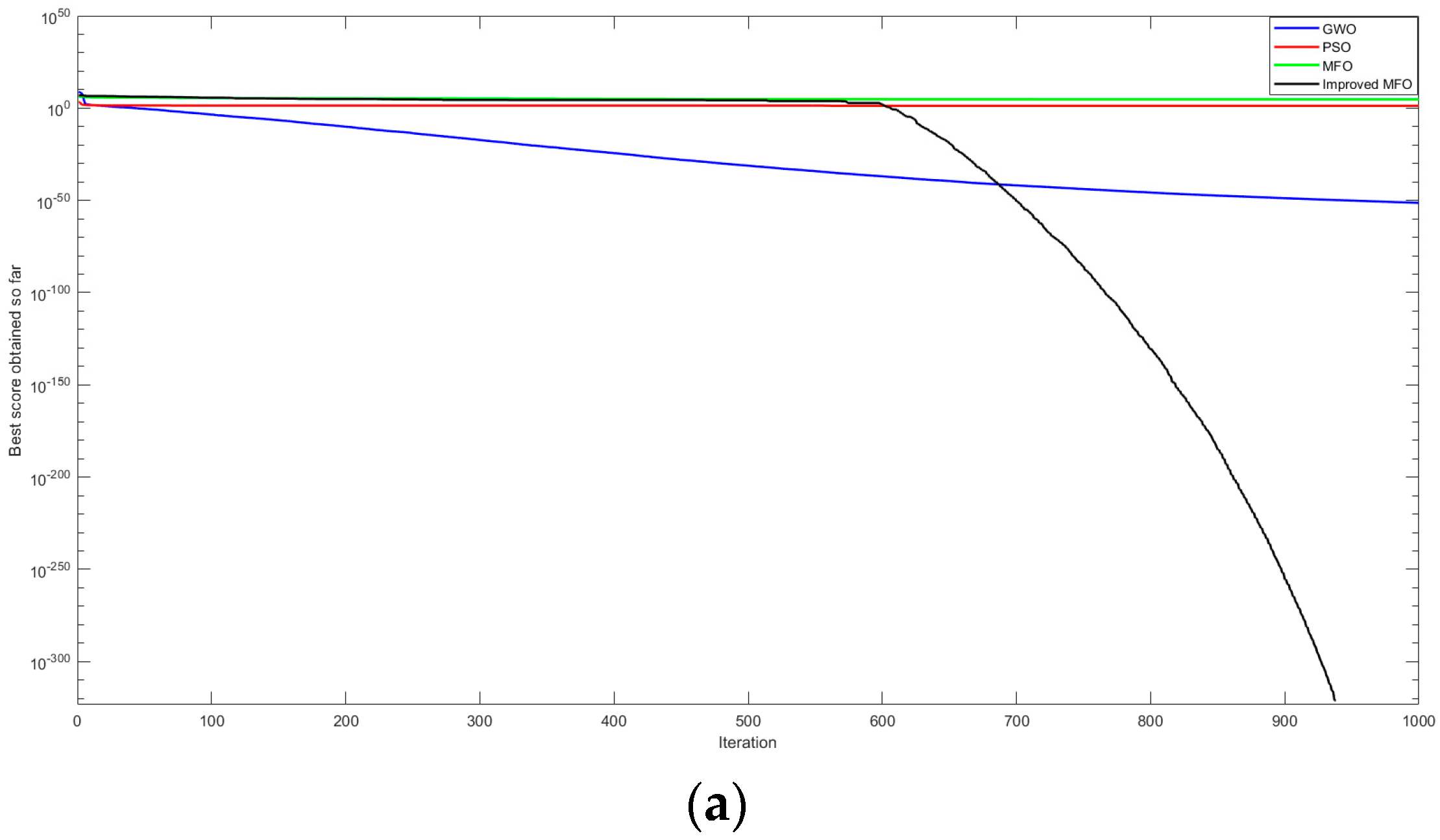
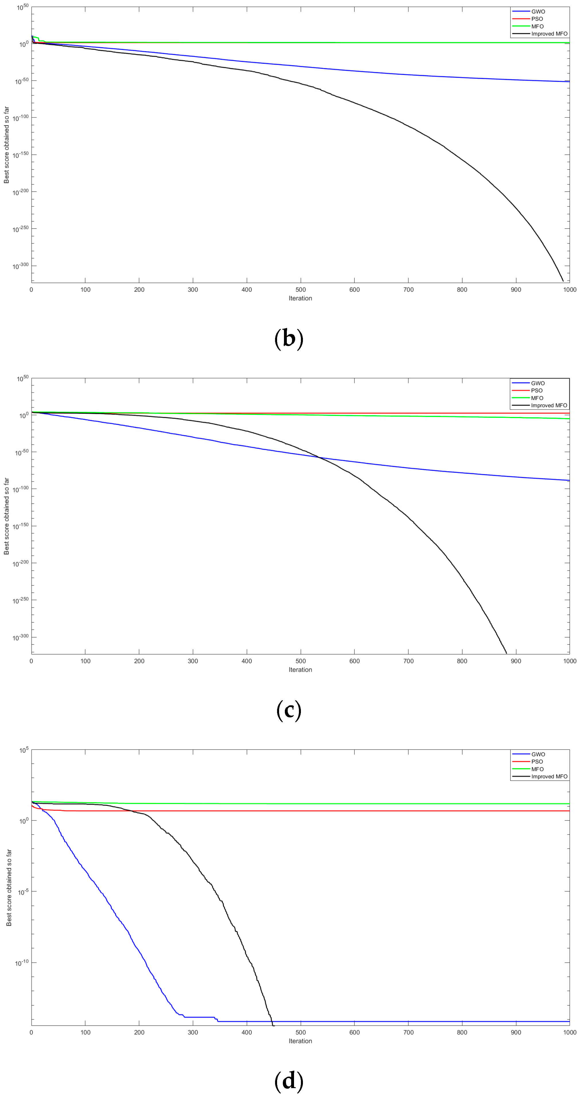
To verify the effectiveness and superiority of the improved MFO algorithm, four commonly used functions were selected for the test, and the dimensions for the tested functions are all 30. The tested functions are given as follows.

8.

(1) Schwefel’s Problem 1.2 function

$$f_1(x)={{\displaystyle {\sum }_{i=1}^{\mathrm{d}}({\displaystyle {\sum }_{j=1}^i{x}_j})}}^2$$

(15)

where;$x_i\in [-100,100]$, and the optimal value of this function is 0.

(2) Schwefel’s Problem 2.22 function

$$f_2(x)={\displaystyle {\sum }_{i=1}^d\left|x_i\right|}+{\displaystyle {\prod }_{i=1}^d\left|x_i\right|}$$

(16)

where; $x_i\in [-10,10]$, and the optimal value of this function is 0.

(3) Sum Squares function

$$f_3(x)={\displaystyle {\sum }_{i=1}^{d}i{x}_i^2}$$

(17)

where; $x_i\in [-10,10]$, and the optimal value of this function is 0.

(4) Ackley function

$$f_4(x)=-20\exp \left(-0.2\sqrt{\frac{1}{d}{\displaystyle {\sum }_{i=1}^d{x}_i^2}}\right)-\exp \left(\frac{1}{d}{\displaystyle {\sum }_{i=1}^d\cos (2\pi x_i)}\right)+20+e$$

(18)

where; $x_i\in [-32,32]$, and the optimal value of this function is 0.

In the verification, the moth population is set to consist of 30 individuals, with a maximum of 1000 iterations; the parameters m and $p$ in the crossover operator are set as 15 and 5, respectively, which indicates that the first 15 flame positions after sorting are disordered five times. Each tested function was performed 20 times, and the results are compared with those obtained from the original MFO, GWO, and PSO optimization algorithms. A summary of the comparison results is shown in

Table 1. Test results of the four algorithms.

Test Function	Optimization Method	Optimal Value	Average Value	Standard Deviation
f1	MFO	1.805 × 103	2.267 × 104	1.206 × 104
	PSO	1.733 × 103	6.425 × 103	4.266 × 103
	GWO	4.375 × 10−30	1.048 × 10−22	3.188 × 10−22
	Improved MFO	0	0	0
f2	MFO	1.786 × 10−5	37.001	24.516
	PSO	9.450	17.299	7.075
	GWO	5.2215 × 10−53	3.959 × 10−52	3.899 × 10−52
	Improved MFO	0	0	0
f3	MFO	4.436 × 10−6	366.667	441.262
	PSO	97.068	297.065	92.301
	GWO	9.625 × 10−93	9.744 × 10−88	3.885 × 10−87
	Improved MFO	0	0	0
f4	MFO	0.9313	17.3889	5.0531
	PSO	4.001	5.156	0.563
	GWO	7.105 × 10−15	1.042 × 10−14	2.787 × 10−15
	Improved MFO	0	0	0

.

The iterative optimization convergence curves of MFO, GWO, and PSO are shown in Figure 2. Additionally, Table 1 illustrates that the improved MFO algorithm exhibits superior optimization capability compared to three other algorithms. It produces the highest optimization accuracy across four test functions and is able to identify global optimal values. These findings provide convincing evidence that the algorithm improvement was effective.

4. VMD Optimization Based on the Improved MFO

4.1. Optimal Process

Modal aliasing may likely occur if the VMD decomposition process is accompanied by improperly chosen parameters [40]. To prevent the influence of artificial parameters, the improved MFO algorithm is implemented in the parameter selection process of VMD to achieve the adaptive selection of the critical parameters of VMD.

This paper employs envelope entropy to describe the coefficient characteristics of signals. A smaller envelope entropy indicates more regular fault pulses [27]. Thus, the minimum average envelope entropy (MAEE) is utilized as the fitness function, which is defined as:

$$p_i(n)=\frac{a_i(n)}{{\displaystyle {\sum }_{n=1}^N{a}_i(n)}}$$

(19)

$$H_{en}\left(i\right)=-{\displaystyle {\sum }_{n=1}^N{p}_i(n){\log }_2(p_i(n))}$$

(20)

$$MAEE=\underset{(K,\alpha )}{\min }\left\{\frac{1}{K}{\displaystyle {\sum }_{i=1}^K{H}_{en}(i)}\right\}$$

(21)

where; a_i(n) is the envelope signal of the i—th modal component, $p_i(n)$ is the normalized form of $a_i(n)$, and $H_{en}(i)$ is the envelope entropy value of the $i-th$ modal component.

After the original signal has been subjected to VMD decomposition, it gives rise to several modal components. The efficacy of the decomposition can be evaluated through determination of the average envelope entropy of each modal component. A decrease in the average envelope entropy value indicates a reduction in noise signals in the decomposed modal components, yielding more consistent fault pulses.

The specific process of the MFO-optimized VMD proposed in this paper is as follows:

(1)

The moth population and flame matrix are initialized, and MAEE was used as fitness function.

(2)

VMD decomposition was performed on the position of each moth to obtain the fitness value of each moth. The moth population was sorted according to the fitness value, and the former flameno flames were selected to construct the matrix.

(3)

Select the first m flame and any flame for $p$ times cross recombination, and, if the fitness value of the new flame is better than the original flame, the original flame is replaced.

(4)

Equation (14) was used to update the moth population position, and VMD decomposition was performed on the signal in the new position of each moth to calculate the fitness value of each moth and update the moth population and flame population.

(5)

The algorithm determines whether the pre-determined number of iterations has been reached. In case it has not, the algorithm repeats the process in steps 2 to 4. When the predetermined number of iterations has been reached, the iteration stops, and the optimal configuration of parameters is presented as output.

4.2. IMF Screening Based on the $EWCS$

When the value of $K$ is greater than the number of components in the signal, over-decomposition occurs. False IMFs may exist among the K IMFs components of the original signal when decomposed by the MFO-optimized VMD method. These false components can adversely affect subsequent fault classification. Therefore, it is necessary to separate these false IMF components. While correlation coefficients or kurtosis criteria are frequently employed in separating false IMFs by existing methods [41], these indicators may not fully capture the intricate vibration characteristics of signals [42]. To address this limitation, we propose a novel evaluation index, known as the $EWCS$, to screen IMFs. A modal component with a calculated $EWCS$ greater than 0 is identified as an effective one. The $EWCS$ calculation involves both the correlation coefficient and sparsity of the IMF, providing a more comprehensive assessment of its suitability. The $EWCS$ is calculated using the formula:

$$Spa=\frac{\sqrt{\frac{1}{N}{\displaystyle {\sum }_{i=1}^N{x}^2(t)}}}{\frac{1}{N}{\displaystyle {\sum }_{i=1}^N\left|x(t)\right|}}$$

(22)

$$Cor=\frac{E[(x-\overline{x})(y-\overline{y})]}{E[{(x-\overline{x})}^2]E[{(y-\overline{y})}^2]}$$

(23)

$$WCS=Spa\cdot Cor$$

(24)

$$EWCS(i)=WCS(i)-\frac{1}{K}{\displaystyle {\sum }_{i=1}^{K}WCS(i)}$$

(25)

where; $Spa$ is the sparsity of signal $x(t)$, and $Cor$ is the correlation coefficient between signal $x$ and $y$.

4.3. Simulated Analysis

A mathematical model was utilized to simulate the signal of rolling bearing inner ring faults for the purpose of evaluating the effectiveness of the MFO-optimized VMD method and the $EWCS$ index:

$$x(t)=s(t)+n(t)={\displaystyle {\sum }_i{A}_{i}h}(t-iT-{\tau }_i)+n(t)$$

(26)

$$h(t)=\exp (-Ct)\cos (2\pi f_{n}t)$$

(27)

$$A_i=1+A_0\cos (2\pi f_{r}t)$$

(28)

The simulation signal was synthesized by adding a periodic impact component $s(t)$ with Gaussian white noise $n(t)$. The sampling frequency ($f_s$) was set to 12,000 Hz, while the rotation frequency ($f_r$), the structural resonance frequency ($f_n$), the fault frequency ($f_i$), and the damping ratio ($C$) were set to 33 Hz, 3000 Hz, 79 Hz, and 500, respectively. Additionally, the signal-to-noise ratio (SNR) of the Gaussian white noise was set as −5 dB. The resulting simulation signal was plotted in both the time domain and the envelope spectrum, as presented in Figure 3.

Figure 3 shows that the periodic impact characteristics that resulted from the structure failure are enveloped by noise, which makes it difficult to extract the impact characteristics precisely and directly. As such, signal processing techniques are necessary to extract the impact characteristics.

The optimal parameter combination for VMD was determined using the improved MFO. Initially, we set the population size to 20 and a maximum of 10 iterations, with $m$ and $p$ values both set to 10. The outcome of the parameter search is illustrated in Figure 4.

Figure 4 demonstrates that the MAEE value of 9.2493800, achieved with parameter combination <3, 773>, was obtained on the third iteration. To demonstrate the proposed improved MFO algorithm’s efficiency, we compared its performance to three other popular optimization algorithms: the original MFO, GWO, and PSO. Each algorithm had an initial population size of 20 and was restricted to a maximum of 10 iterations. Each algorithm ran for 10 iterations, and

Table 2. Results of four optimization algorithms.

Algorithm	Optimum Value	MSE	STD
GWO	9.249382	7.2257 × 10−12	1.8724 × 10−15
PSO	9.249380	1.1715 × 10−6	7.2087 × 10−4
MFO	9.249380	1.9533 × 10−7	4.4167 × 10−4
Improved MFO	9.249380	5.9336 × 10−12	1.5860 × 10−6

presents the results obtained.

Table 2 reveals that GWO exhibits the highest MAEE value amongst the four algorithms across the ten operations. Despite the fact that the MAEE values obtained by the PSO, MFO, and improved MFO3 algorithms are equivalent, the improved MFO algorithm has the smallest mean square error and standard deviation across all results, demonstrating its efficacy.

The optimal parameter combination of <3, 773> was used to decompose the simulation signal by VMD. To validate the proposed EWCS index, we computed the Peak Signal-to-Noise Ratio (PSNR), Mean Squared Error (MSE), and EWCS value of the three resulting IMFs obtained from the decomposition. The computed results are presented in

Table 3. The selection of effective IMF components.

Index	IMF1	IMF2	IMF3
PSNR	52.0958	52.8020	52.2489
MSE	0.4013	0.3411	0.3874
EWCS	−0.0096	0.0276	−0.0180
Effective IMFs		√

, where it can be observed that IMF2 exhibits the highest PSNR and the smallest MSE, thus implying that this IMF contains abundant fault information. This observation is consistent with the outcome of the proposed method, which screens effective IMFs based on EWCS value, and it substantiates the validity of the proposed method.

The effective component IMF2, after being screened, underwent an envelope demodulation analysis and yielded an envelope spectrum displayed in Figure 5. The extracted frequency components included the conversion frequency ($f_r$), the fault characteristic frequency ($f_i$), and its double frequency ($2f_i$). These results demonstrate the successful application of the VMD optimization method proposed in this paper, in combination with EWCS index screening, for effectively decomposing the simulation signal $x(t)$.

To verify the superiority of the proposed method, we employed a VMD decomposition technique with fixed parameters of <5, 2000> and identified effective components as IMF3, IMF4, and IMF5 based on the EWCS (Method 1). Additionally, we utilized the screening method based on correlation coefficient and kurtosis value, presented in reference [43], along with a <3, 773> VMD decomposition, and we identified IMF1 and IMF2 as effective components (Method 2). Subsequently, we reconstructed and analyzed the selected effective components using envelope demodulation, and the outcomes are illustrated in Figure 6.

Figure 6 indicates that Method 1 and Method 2 were unable to extract $f_r$ and $f_i$. By contrast, the VMD optimization method and EWCS index utilized in the proposed method were successful in extracting signal components that carried the information on system faults. This finding reinforces the effectiveness of the VMD optimization method and the EWCS index in fault feature extraction.

5. The Diagnosis Method Based on MFO-Optimized VMD and DE-OSELM

5.1. The Proposed Method

To begin with, a modification of MFO is utilized to enable adaptive selection of VMD parameters, thereby avoiding the influence of manually set parameters on VMD decomposition effect. The decomposed IMFs are screened using the EWCS index. Given that the energy levels of individual components of the vibration signal’s IMF differ based on the rolling bearing’s distinct movement states, the energy attributes of these components are isolated to develop a feature matrix. Lastly, the energy eigenmatrix is input into DE-OSELM in order to perform fault classification using the principles outlined in reference [37]. Figure 7 shows the flow chart for our proposed method.

The specific process is listed as follows:

(1)

The improved MFO was used to optimize $K$ and $\alpha$ in VMD parameters, and the optimal parameter combination $(k_0,{\alpha }_0)$ was obtained.

(2)

The VMD with optimized parameters was used to process the collected signals, and $K$ IMFs were decomposed.

(3)

The EWCS index was used to screen $K$ IMFs, eliminate the false IMFs, extract the energy features of effective IMFs, and form the feature vector matrix.

(4)

The energy feature matrix is normalized and input into DE-OSELM for training and fault classification.

5.2. Experimental Verification

To assess the effectiveness and superiority of MFO-optimized VMD and DE-OSELM for detecting faults in rolling bearings, we conducted an experiment using actual operation data of the 6205 deep groove ball bearing type obtained from Western Reserve University’s laboratory [44]. As illustrated in Figure 8, the simulation test bench for rolling bearing faults features a pitch circle diameter of 39.04 mm, as well as nine rolling bodies with a diameter of 7.94 mm each and 0°contact angle. The vibration signals were collected under four operating states: normal, inner ring failure, outer ring failure, and rolling body failure. We shifted 100 groups of vibration signals for each state, with each group consisting of 1024 signal lengths, resulting in a total of 400 groups.

Ten groups of normal signals were randomly selected for the experiment. The improved MFO algorithm was initiated with an initial population size of 30. The maximum number of iterations was set as 10, with m = 10 and p = 5. $K$ and $\alpha$ values were ranged between [4, 12] and [800, 3000]. Figure 9 shows the search results, and the optimized values for $K$ and $\alpha$ were determined to be 10 and 924, respectively.

The EWCS index was utilized to screen the decomposed IMFs, and the EWCS values of each modal component for the ten groups of signals were presented in

Table 4. The value of EWCS of each IMF for 10 groups of normal signals.

Number	IMF1	IMF2	IMF3	IMF4	IMF5	IMF6	IMF7	IMF8	IMF9	IMF10
1	0.2567	0.1588	0.6992	−0.0227	−0.1525	−0.1820	−0.1846	−0.1875	−0.1905	−0.1951
2	0.2619	0.1511	0.6659	−0.0330	−0.0545	−0.1871	−0.1900	−0.1962	−0.1995	−0.2186
3	0.2429	0.6247	0.6202	−0.0846	−0.1055	−0.2465	−0.2558	−0.2649	−0.2573	−0.2732
4	0.2742	0.6095	0.6110	−0.0691	−0.1873	−0.2306	−0.2464	−0.2468	−0.2514	−0.2632
5	0.3334	0.1268	0.6938	−0.0299	−0.1616	−0.1851	−0.1863	−0.1892	−0.1988	−0.2030
6	0.2352	0.6979	0.6859	−0.0878	−0.2282	−0.2492	−0.2538	−0.2660	−0.2597	−0.2743
7	0.1517	0.5070	0.6256	−0.0689	0.0619	−0.2390	−0.2522	−0.2584	−0.2535	−0.2742
8	0.3234	0.1465	0.6228	−0.0174	−0.0514	−0.1945	−0.2002	−0.2091	−0.2042	−0.2158
9	0.2809	0.5466	0.5914	−0.0520	−0.2003	−0.2183	−0.2371	−0.2374	−0.2332	−0.2408
10	0.2337	0.1156	0.7296	−0.0069	−0.1555	−0.1727	−0.1865	−0.1843	−0.1828	−0.1902
Effective IMFs	√	√	√

. Based on the screening outcomes of the ten groups of signals, the effective components of IMF1, IMF2, and IMF3 were identified.

VMD decomposition was performed using K values of 10 and 924 on 400 sets of vibration signals in four different states. The energy characteristics of IMF1, IMF2, and IMF3 were extracted, resulting in an eigenvector matrix that was normalized. Adding labels produced a 400 × 4 eigenmatrix. The energy characteristic matrix was randomly partitioned into training and test sets at a ratio of 3:1, resulting in 300 training samples and 100 test samples. After VMD decomposition, the components of the reconstructed signal were simpler, and the fault frequency was more obvious. Figure 10 shows the spectrum diagram of the original signal and reconstructed signal with the rolling element fault.

Parameter settings used in the DE algorithm consisted of NP = 20, F = 0.5, and CR = 0.75 [37]. The performance of the OSELM algorithm is affected by the choice of activation function. Therefore, to shorten the training time, which is twice as long as that of OSELM with RBF activation [32], the Sigmoid function was selected as the activation function for OSELM. The number of nodes in its hidden layer and bias range were set to 25 and [0, 1], respectively. The input weight was constrained to [−1, 1]. An amount of 50 training data were used initially, and each learning data block in the following step contained 40 data.

The OSELM and DE-OSELM were implemented to investigate the robustness of the latter, with 30 experiments conducted for each group. The experiment results presented in Figure 11 demonstrate the superior classification accuracy of DE-OSELM, as compared to OSELM, indicating better robustness.

To substantiate the efficacy of this approach, the results obtained from Fixed Parameter <8, 2000> VMD and MFO-optimized VMD were fed into several machine learning models, namely, ELM, OSELM, KNN, and DE-OSELM, to recognize and classify the data. We repeated the experiment 30 times to ensure its reliability. Classification outcomes of the proposed approach, as well as the other three methodologies, are showcased in

Table 5. The comparison of classification accuracy of the four methods.

Classify	<8, 2000> VMD	MFO-Optimized VMD
ELM	92.67%	96.17%
OSELM	92.70%	96.40%
KNN	88.00%	99.00%
DE-OSELM	99.73%	100%

. The results demonstrate that the accuracy of classification achieved through the proposed method is notably better than the other three methods, affirming the efficacy and superiority of the proposed method.

5.3. Diagnostic Case Analysis

The viability and effectiveness of the proposed approach were evaluated using the drivetrain dynamics simulator (DDS), as illustrated in Figure 12, manufactured by SpectraQuest [45]. The ER-16K rolling bearing type was utilized to obtain the corresponding vibration signals. The bearing had a pitch circle with a 15.16 mm diameter, nine rolling bodies with a diameter of 3.125 mm, and a contact angle of 0°. The experiment was conducted with a motor frequency of 20 Hz, zero load, a sampling frequency of 12,800 Hz, and a sampling length of 200 KiB. Vibrations were captured under four operating conditions: normal operation, inner ring failure, outer ring failure, and rolling body failure. A total of 400 signals were recorded, consisting of 100 sets of vibration signals for each of the four operating conditions, with a signal length of 1024 samples per group.

Ten groups of normal signals were randomly selected for this study, and their decomposition layers and quadratic penalty factor were optimized through the improved MFO algorithm to obtain an optimal combination of <10, 1535>. The VMD algorithm was then applied to decompose each signal using this optimized parameter combination, after which the EWCS value of each IMF was calculated. The findings are presented in

Table 6. The value of the EWCS of each IMF for 10 groups of normal signals.

Number	IMF1	IMF2	IMF3	IMF4	IMF5	IMF6	IMF7	IMF8	IMF9	IMF10
1	0.0278	0.4454	0.0871	0.1326	0.0537	0.0165	−0.1641	−0.1761	−0.2020	−0.2209
2	−0.0127	0.2431	0.3095	0.1650	0.0614	−0.0283	−0.1590	−0.1753	−0.1918	−0.2118
3	0.0611	0.3306	0.2607	0.1559	0.0237	−0.0913	−0.1882	−0.1716	−0.1823	−0.1985
4	0.0243	0.2993	0.3166	0.1179	0.0566	−0.0794	−0.1805	−0.1891	−0.1802	−0.1855
5	0.1275	0.4619	0.1291	0.0676	−0.0368	−0.0952	−0.1517	−0.1502	−0.1724	−0.1798
6	0.0274	0.5054	0.1340	0.1041	−0.0280	−0.1411	−0.1289	−0.1295	−0.1700	−0.1733
7	−0.0157	0.4426	0.1010	0.0586	0.0445	−0.0090	−0.1345	−0.1454	−0.1733	−0.1688
8	0.0704	0.5200	0.1909	0.0291	0.0018	−0.1494	−0.1634	−0.1509	−0.1732	−0.1753
9	0.0525	0.4863	0.0815	0.0608	−0.0111	−0.0304	−0.1660	−0.1417	−0.1570	−0.1749
10	−0.0823	0.3017	0.2943	0.1209	0.0768	0.0123	−0.1820	−0.1602	−0.1963	−0.1851
Effective IMFs	√	√	√	√	√

. After VMD decomposition, the components of the reconstructed signal were simpler, and the fault frequency was more obvious. Figure 13 shows the spectrum diagram of the original signal and reconstructed signal with the rolling element fault.

The feature matrix is input into both OSELM and DE-OSELM classification models, and their respective classification results are presented in Figure 14. Accordingly, it is evident from the figure that DE-OSELM achieves higher classification accuracy than OSELM, further reinforcing the effectiveness and universality of DE-OSELM. This comparison result provides robust evidence to support the superiority of DE-OSELM in classification performance.

To validate the efficacy of our proposed technique, we input the results of both the fixed parameter <7, 2000> VMD and the MFO-optimized VMD into four distinct classification algorithms—ELM, OSELM, KNN, and DE-OSELM—for classification and recognition purposes.

Table 7. Comparison of classification accuracy of the four methods.

Classify	<7, 2000> VMD	MFO-Optimized VMD
ELM	90.37%	91.33%
OSELM	90.97%	91.07%
KNN	91.00%	93.00%
DE-OSELM	97.43%	98.80%

displays the classification outcomes of the four techniques. Table 7 supports the efficacy of the proposed MFO-optimized VMD and DE-OSELM diagnostic methods, which demonstrate greater accuracy and reliability compared to the other three methods.

At the same time, it is compared with two existing fault diagnosis methods, namely, the fault diagnosis method, based on EMD and OSELM [46], the fault diagnosis method, based on VMD and KNN [47], and results are shown in

Table 8. Fault classification accuracy of three methods.

Fault Diagnosis Method	Accuracy Rate %
EMD and OSELM	92.70
VMD and KNN	97.13
improved VMD and DE-OSELM	98.80

. From the results, we can see that their classification accuracy scores. The differences are 92.7% and 97.13%, and, compared with the improved VMD and DE-OSELM diagnostic methods proposed in this paper, these are higher. This also further verifies the effectiveness and superiority of the proposed method.

6. Conclusions

Two novel methods for diagnosing rolling bearing faults have been proposed, MFO-optimized VMD and DE-OSELM. The objective of these methods are to tackle the challenge of signal degradation, caused by environmental noise, which presents difficulties in identifying subtle fault features. The method presented in this paper presents a new idea for fault diagnosis of rolling bearings.

(1)

The original MFO algorithm is subject to low accuracy and slow convergent speed, probably due to falling into the local optimal solution. This issue is solved through the proposed dynamic adaptive weight factor and crossover operator, which significantly improves the algorithm’s global optimization ability.

(2)

The traditional VMD decomposition method faces a challenge of modal aliasing due to suboptimal selection of critical parameters, including the number of decomposition layers and quadratic penalty factor. To address this problem, this study introduces an improved MFO algorithm, utilizing the Mean Absolute Envelope Error (MAEE) as the fitness function, to adaptive select these two parameters and effectively improve the quality of VMD decomposition.

(3)

False IMF components generated by VMD decomposition are removed using the EWCS index. The real components containing fault feature information are subsequently extracted.

(4)

This study proposes a fault diagnosis method that utilizes MFO-optimized VMD and DE-OSELM. Numerical analysis and field test data analysis were conducted to verify the effectiveness and feasibility of the proposed method. Our results demonstrate that the proposed approach displays superior anti-noise performance and accuracy in fault identification when compared to other commonly used diagnostic techniques.

References

1. He, C.; Liu, C.; Wu, T.; Xu, Y.; Wu, Y.; Chen, T. Medical rolling bearing fault prognostics based on improved extreme learning machine. J. Comb. Optim. Vol. 2021, 42, 700–721. [Google Scholar] [CrossRef]
2. Wang, B.; Wen, L.; Li, X.; Gao, L. Adaptive Class Center Generalization Network: A Sparse Domain-Regressive Framework for Bearing Fault Diagnosis under Unknown Working Conditions. IEEE Trans. Instrum. Meas. 2023, 72, 3516511. [Google Scholar] [CrossRef]
3. Zhang, Y.; Qin, Y.; Du, Y.P.; Zhu, L.; Wei, X.K. Railway vehicle bearings risk monitoring based on normal region estimation for no-fault data situations. J. Transp. Saf. Secur. 2021, 10, 1047–1065. [Google Scholar] [CrossRef]
4. Saufi, S.R.; Ahmad, Z.A.B.; Leong, M.S.; Lim, M.H. An intelligent bearing fault diagnosis system. MATEC Web Conf. 2019, 255, 06005. [Google Scholar] [CrossRef]
5. Guo, X.; Shen, C.; Chen, L. Deep fault recognizer: An integrated model to denoise and extract features for fault diagnosis in rotating machinery. Appl. Sci. 2017, 7, 41. [Google Scholar] [CrossRef] [Green Version]
6. Golafshan, R.; Sanliturk, K.Y. SVD and Hankel matrix based de-noising approach for ball bearing fault detection and its assessment using artificial faults. Mech. Syst. Signal Process. 2016, 70–71, 36–50. [Google Scholar] [CrossRef]
7. Wen, L.; Li, X.; Gao, L. A new reinforcement learning based learning rate scheduler for convolutional neural network in fault classification. IEEE Trans. Ind. Electron. 2020, 68, 12890–12900. [Google Scholar] [CrossRef]
8. Yan, R.; Gao, R.X. Hilbert-Huang transform-based vibration signal analysis for machine health monitoring. IEEE Trans. Instrum. Meas. 2006, 55, 2320–2329. [Google Scholar] [CrossRef]
9. Huang, N.E.; Shen, Z.; Long, S.R.; Wu, M.C.; Shih, H.H.; Zheng, Q.; Yen, N.-C.; Tung, C.C.; Liu, H.H. The empirical mode decomposition and the Hilbert spectrum for nonlinear and non-stationary time series analysis. Proc. R. Soc. Lond. Ser. A Math. Phys. Eng. Sci. 1998, 454, 903–995. [Google Scholar] [CrossRef]
10. Dybata, J.; Zimroz, R. Rolling bearing diagnosing method based on empirical mode decomposition of machine vibration signal. Appl. Acoust. 2014, 77, 195–203. [Google Scholar]
11. Guo, T.; Deng, Z.M. An improved EMD method based on the multi-objective optimization and its application to fault feature extraction of rolling bearing. Appl. Acoust. 2017, 127, 46–62. [Google Scholar] [CrossRef]
12. Wu, Z.H.; Huang, N.E. Ensemble empirical mode decomposition: A noise-assisted data analysis method. Adv. Adapt. Data Anal. 2009, 1, 1–41. [Google Scholar] [CrossRef]
13. Lei, Y.G.; He, Z.J.; Zi, Y.Y. Application of the EEMD method to rotor fault diagnosis of rotating machinery. Mech. Syst. Signal Process. 2009, 23, 1327–1338. [Google Scholar] [CrossRef]
14. Jiang, H.K.; Li, C.L.; Li, H.X. An improved EEMD with multiwavelet packet for rotating machinery multi-fault diagnosis. Mech. Syst. Signal Process. 2013, 36, 225–239. [Google Scholar] [CrossRef]
15. Smith, J.S. The local mean decomposition and its application to EEG perception data. J. R. Soc. Interface 2005, 2, 443–454. [Google Scholar] [CrossRef]
16. Cheng, J.S.; Yang, Y.; Yang, Y. A rotating machinery fault diagnosis method based on local mean decomposition. Digit. Signal Process. 2012, 22, 356–366. [Google Scholar] [CrossRef]
17. Wang, Z.; Wang, J.; Cai, W.; Zhou, J.; Du, W.; Wang, J.; He, G.; He, H. Application of an improved ensemble local mean decomposition method for gearbox composite fault diagnosis. Complexity 2019, 2019, 1564243. [Google Scholar] [CrossRef] [Green Version]
18. Dragomiretskiy, K.; Zosso, D. Variational mode decomposition. IEEE Trans. Signal Process. 2014, 62, 531–544. [Google Scholar] [CrossRef]
19. Jiang, X.; Song, Q.; Wang, H.; Du, G.; Guo, J.; Shen, C.; Zhu, Z. Central frequency mode decomposition and its applications to the fault diagnosis of rotating machines. Mech. Mach. Theory 2022, 174, 104919. [Google Scholar] [CrossRef]
20. Gharehbaghi, V.R.; Kalbkhani, H.; Farsangi, E.N.; Yang, T.Y.; Mirjalili, S. A data-driven approach for linear and nonlinear damage detection using variational mode decomposition and GARCH model. Eng. Comput. 2022, 39, 2017–2034. [Google Scholar] [CrossRef]
21. Bagheri, A.; Ozbulut, O.E.; Harris, D.K. Structural system identification based on variational mode decomposition. J. Sound Vib. 2018, 417, 182–197. [Google Scholar] [CrossRef]
22. Li, K.; Su, L.; Wu, J.; Wang, H.; Chen, P. A rolling bearing fault diagnosis method based on variational mode decomposition and an improved kernel extreme learning machine. Appl. Sci. 2017, 7, 1004. [Google Scholar] [CrossRef] [Green Version]
23. Wang, C.; Li, H.; Huang, G.; Ou, J. Early fault diagnosis for planetary gearbox based on adaptive parameter optimized VMD and singular kurtosis difference spectrum. IEEE Access 2019, 7, 31501–31516. [Google Scholar] [CrossRef]
24. Tang, G.J.; Wang, X.L. Parameter optimized variational mode decomposition method with application to incipient fault diagnosis of rolling bearing. J. Xi’an Jiaotong Univ. 2015, 49, 73–81. [Google Scholar]
25. Zhang, X.; Miao, Q.; Zhang, H.; Wang, L. A parameter-adaptive VMD method based on grasshopper optimization algorithm to analyze vibration signals from rotating machinery. Mech. Syst. Signal Process. 2018, 108, 58–72. [Google Scholar] [CrossRef]
26. Gu, R.; Chen, J.; Hong, R.; Wang, H.; Wu, W. Incipient fault diagnosis of rolling bearings based on adaptive variational mode decomposition and Teager energy operator. Measurement 2020, 149, 106941. [Google Scholar] [CrossRef]
27. Mirjalili, S. Moth-Flame Optimization Algorithm: A Novel NatureInspired Heuristic Paradigm. Knowl. Based Syst. 2015, 89, 228–249. [Google Scholar] [CrossRef]
28. Yildiz, B.; Yildiz, A.R. Moth-flame optimization algorithm to determine optimal machining parameters in manufacturing processes. Mater. Test. 2017, 59, 425–429. [Google Scholar] [CrossRef]
29. Wei, J.; Huang, H.; Yao, L.; Hu, Y.; Fan, Q.; Huang, D. New imbalanced fault diagnosis framework based on Cluster-MWMOTE and MFO-optimized LS-SVM using limited and complex bearing data. Eng. Appl. Artif. Intell. 2020, 96, 103966. [Google Scholar] [CrossRef]
30. Sivalingam, V.; Sun, J.; Mahalingam, S.K.; Nagarajan, L.; Natarajan, Y.; Salunkhe, S.; Nasr, E.A.; Davim, J.P.; Hussein, H.M.A.M. Optimization of process parameters for turning hastelloy X under different machining environments using evolutionary algorithms: A comparative study. Appl. Sci. 2021, 11, 9725. [Google Scholar] [CrossRef]
31. Chen, W.; Li, J.; Wang, Q.; Han, K. Fault feature extraction and diagnosis of rolling bearings based on wavelet thresholding denoising with CEEMDAN energy entropy and PSO-LSSVM. Measurement 2021, 172, 108901. [Google Scholar] [CrossRef]
32. Huang, G.B.; Zhu, Q.Y.; Siew, C.K. Extreme learning machine: A new learning scheme of feedforward neural networks. In Proceedings of the IEEE International Joint Conference on Neural Networks, Budapest, Hungary, 25–29 July 2004; IEEE: Piscataway, NJ, USA, 2005; pp. 489–501. [Google Scholar]
33. Jiang, G.; Xie, P.; Du, S.; Guo, Y.; He, Q. A new fault diagnosis model for rotary machines based on MWPE and ELM. Insight-Non-Destr. Test. Cond. Monit. 2017, 59, 644–652. [Google Scholar] [CrossRef]
34. Lan, Y.; Hu, J.; Huang, J.; Niu, L.; Zeng, X.; Xiong, X.; Wu, B. Fault diagnosis on slipper abrasion of axial piston pump based on extreme learning machine. Measurement 2018, 124, 378–385. [Google Scholar] [CrossRef]
35. Liang, N.Y.; Huang, G.B.; Saratchandran, P.; Sundararajan, N. A fast and accurate online sequential learning algorithm for feedforward networks. IEEE Trans. Neural Netw. 2006, 17, 1411–1423. [Google Scholar] [CrossRef] [PubMed]
36. Sahani, M.; Dash, P.K.; Samal, D. A real-time power quality events recognition using variational mode decomposition and online-sequential extreme learning machine. Measurement 2020, 157, 107597. [Google Scholar] [CrossRef]
37. Zhou, Z.; Gao, X.; Zhang, J.; Zhu, Z.; Hu, X. A novel hybrid model using the rotation forest-based differential evolution online sequential extreme learning machine for illumination correction of dyed fabrics. Text. Res. J. 2018, 89, 1180–1197. [Google Scholar] [CrossRef]
38. Mao, W.; Feng, W.; Liang, X. A novel deep output kernel learning method for bearing fault structural diagnosis. Mech. Syst. Signal Process. 2019, 117, 293–318. [Google Scholar] [CrossRef]
39. Yan, X.; Liu, Y.; Zhang, W.; Jia, M.; Wang, X. Research on a novel improved adaptive variational mode decomposition method in rotor fault diagnosis. Appl. Sci. 2020, 10, 1696. [Google Scholar] [CrossRef] [Green Version]
40. Li, H.; Fan, B.; Jia, R.; Zhai, F.; Bai, L.; Luo, X. Research on multi-domain fault diagnosis of gearbox of wind turbine based on adaptive variational mode decomposition and extreme learning machine algorithms. Energies 2020, 13, 1375. [Google Scholar] [CrossRef] [Green Version]
41. Deng, W.; Liu, H.; Zhang, S.; Liu, H.; Zhao, H.; Wu, J. Research on an adaptive variational mode decomposition with double thresholds for feature extraction. Symmetry 2018, 10, 684. [Google Scholar] [CrossRef] [Green Version]
42. Zhang, X.; Wan, S.; He, Y.; Wang, X.; Dou, L. Teager energy spectral kurtosis of wavelet packet transform and its application in locating the sound source of fault bearing of belt conveyor. Measurement 2021, 173, 108367. [Google Scholar] [CrossRef]
43. Fu, Q.; Jing, B.; He, P.; Si, S.; Wang, Y. Fault feature selection and diagnosis of rolling bearings based on EEMD and optimized Elman_AdaBoost algorithm. IEEE Sens. J. 2018, 18, 5024–5034. [Google Scholar] [CrossRef]
44. CWRU. The Case Western Reserve University Bearing Data Center. 2015. Available online: https://engineering.case.edu/bearingdatacenter/welcome (accessed on 12 November 2022).
45. SpectraQuest. Drivetrain Diagnostics Simulator. 4 January 2018. Available online: http://spectraquest.com/drivetrains/details/dds/ (accessed on 12 November 2022).
46. Xu, X.; An, M.; Cao, S.; Lu, L.; Su, L.; Yang, T.; Luo, J. Non-linear and Non-steady Time Series Forecasting Method Based on EMD and OSELM. Int. J. Netw. Secur. 2023, 25, 61–67. [Google Scholar]
47. Lu, Q.; Shen, X.; Wang, X.; Li, M.; Li, J.; Zhang, M. Fault diagnosis of rolling bearing based on improved VMD and KNN. Math. Probl. Eng. 2021, 2021, 2530315. [Google Scholar] [CrossRef]
Figure 1. The flowchart of the improved MFO.
Applsci 13 07500 g001
Figure 2. The iterative optimization convergence curves of MFO, GWO, and PSO. (a) f1, (b) f2, (c) f3, and (d) f4.
Applsci 13 07500 g002aApplsci 13 07500 g002b
Figure 3. (a) Time–domain of the simulation signal. (b) Frequency–domain diagram of the simulation signal.
Applsci 13 07500 g003
Figure 4. The improved MFO convergence curve of the simulation signal.
Applsci 13 07500 g004
Figure 5. The effective component envelope spectrum.
Applsci 13 07500 g005
Figure 6. (a) The envelope spectrum by method-1. (b) The envelope spectrum by method-2.
Applsci 13 07500 g006
Figure 7. The fault diagnosis process based on the MFO-optimized VMD and DE-OSELM.
Applsci 13 07500 g007
Figure 8. The rolling bearing fault simulation test bench.
Applsci 13 07500 g008
Figure 9. The improved MFO convergence curve of the bearing signal.
Applsci 13 07500 g009
Figure 10. (a) original signal; (b) reconstructed signal.
Applsci 13 07500 g010
Figure 11. Comparison of the DE-OSLEM and OSELM classification results.
Applsci 13 07500 g011
Figure 12. Drivetrain dynamics simulator.
Applsci 13 07500 g012
Figure 13. (a) original signal; (b) reconstructed signal.
Applsci 13 07500 g013
Figure 14. A comparison of the DE-OSLEM and OSELM classification results.
Applsci 13 07500 g014