
Adaptive Fault-Tolerant Control of Hypersonic Vehicles with Unknown Model Inertia Matrix and System Induced by Centroid Shift

1
School of Science, Jiangsu University of Science and Technology, Zhenjiang 212000, China
2
Shanghai Key Laboratory of Aerospace Intelligent Control Technology, Shanghai Aerospace Control Technology Institute, Shanghai 201108, China
*
Author to whom correspondence should be addressed.
Appl. Sci. 2023, 13(2), 830; https://0-doi-org.brum.beds.ac.uk/10.3390/app13020830
Submission received: 15 November 2022
/
Revised: 30 December 2022
/
Accepted: 31 December 2022
/
Published: 6 January 2023
(This article belongs to the Special Issue Advanced Fault Diagnosis and Fault-Tolerant Control Technology of Spacecraft)
Abstract
:In this paper, the fault-tolerant control problem of hypersonic vehicle (HSV) in the presence of unexpected centroid migration, actuator failure and external interference is studied in depth. First, the proposed dynamics for HSV with the aforementioned unexpected factors are modeled to demonstrate the peculiar nature of the subject under study. The adverse effects of accidental centroid migration are mainly reflected in the following aspects: (1) the change of inertia matrix of the system, (2) the uncertainty of the system and (3) the eccentric moment, which are coupled and unknown. Subsequently, to account for the effect of unexpected centroid shifts, a sliding-mode observer and an adaptive estimator are designed to obtain unknowns useful for subsequent FTC controller designs. Later, we derived an innovative adaptive FTC scheme by employing the observer in conjunction with a specific adaptive controller consisting of a sixth-order dynamic compensator, which can guarantee the achievement of the control objective without resorting to the exact knowledge of the inertial matrix. Moreover, the analysis of boundedness with respect to the entire signal in this closed system is performed by means of the Lyapunov stability theory. Ultimately, simulation results show that the proposed FTC strategy is efficient and powerful.
1. Introduction
As a deeply coupled nonlinear aircraft, hypersonic vehicles have the advantages of fast speed, strong maneuverability and good penetration. It has important applications in both military and civil fields, attracting many scholars to study its modeling and controller design [1,2]. The super high speed flight and corresponding complex flight airspace make HSV prone to failure, such as actuator fault, sensor fault, etc. Thus, fault-tolerant control (FTC) systems are central to ensuring HSV safety and achieving its goals.
In a fault event on an aircraft, a significant portion of the aircraft’s aerodynamic lift surface may become detached when it is damaged [3], resulting in an unexpected shift of the aircraft’s center of mass. It is well known that the position of the center of gravity of an aircraft is crucial to the calculation of its control moment [4]. Due to changes in the system, inertia matrix, eccentricity torque and system uncertainty, any unexpected center of gravity movement may put the aircraft in a non-nominal flight state, thus challenging the existing control system to maintain its control performance [3]. A similar situation may arise from fuel consumption, moving mass control [5] as well as the liquid fuel sloshing [6], etc. To ensure the safe flight of the aircraft, adaptive FTC schemes have been developed even in the presence of unexpected centroid shifts, actuator faults and external disturbances.
For variants of aircraft centroids, some previous works deliver the following. An aircraft with unexpected centroid shift is modeled in [7], which is derived from the aircraft body coordinate system, which is not convenient to analyze the influence of centroid migration on HSV flow Angle (Angle of attack and Angle of slip). In addition, a hybrid direct–indirect adaptive control method based on neural network is proposed to deal with the damage-induced centroid migration [7,8]. However, irreversible phenomena may appear in the estimated inertia matrix, leading to singularities in the existing FTC controller resting on the inverse of an inertia matrix. In addition, a linearized aircraft model with centroid shift due to damage is proposed in [9]. Nevertheless, the linearization of the multi-model reference adaptive control makes the system free from the coupling problem caused by centroid migration, leading to a degradation of the control performance. Based on the above studies, the influence of the centroid shift on the HSV motion is mainly reflected in three aspects: (1) the change of inertia matrix of the system, (2) the uncertainty of the system and (3) the eccentric moment, especially in the situation where the inertia matrix appears irreversible. In order to handle the challenge of inertia matrix, RBFNN is adopted in [8] to estimate the inverse of the inertia matrix in order to ensure the normal operation of the controller. To solve this problem, Taylor expansion of the inverse matrix of the inertial matrix is used in [10], but it comes with corresponding Taylor expansion errors and a large number of online computational parameters of the neural network. In addition, Ref. [11] addresses the variation of an inertial matrix by assuming that the minimum and maximum bounds of its eigenvalues are known; however, the mentioned bounds are difficult to measure. With the development of data driven methods [12], a model-free control scheme is developed to handle this challenge, but the training data of the inertial matrix of HSV with centroid-shift is difficult to obtain. Additionally, an observer-based FTC strategy [13], fuzzy approximation [14] and iterative learning [15] are developed to handle this challenge. In summary, how to identify an HSV inertial matrix with uncertainty online and ensure its function in the FTC controller remains elusive.
In the past few decades, the fault-tolerant control of actuators, sensors, control surfaces or other failure systems has been extensively studied, and a large number of FTC control strategies have appeared in the literature. For example, predictive control [1], backstepping control [16], adaptive control [3], fuzzy control [17], control [18] based on neural network, etc. In [16], a second-order system of actuators is established to describe actuator failure (LOE) and stuck faults, which provides a basis for subsequent fault diagnosis and identification (FDI) design.Then, fault-tolerant control strategies resting on FDI and backstepping control are developed to achieve the control objective; however, such accurate actuator models are difficult to establish. In [17], the Takagi–Sugeno (T–S) fuzzy model is applied to describe the attitude dynamics of a near-space vehicle in the case of actuator failure. Then, the adaptive fault-tolerant tracking control is implemented by using the estimated actuator faults, but there is no suitable fuzzy rule to describe the faulty aircraft. In addition, an adaptive output feedback fault-tolerant controller is designed in [19] to handle parameter uncertainties, actuator failures and external disturbances in HSV attitude systems. Therefore, such a large number of adaptive learning parameters can create a heavy online computational load. In addition, based on the strong robustness of sliding mode control and its modified control strategies are more applied in fault-tolerant HSV [20,21]. A new adaptive nonlinear generalized predictive controller is proposed for the longitudinal dynamics of hypersonic vehicles with unknown parameters and constraints [1], showing a good control effect. Nonlinear generalized predictive control [22] shows the good dynamic performance and hugely decreases the computation burden compared with the usual model predictive control. Nonetheless, since inertial matrix variations are not taken into account, they may end up delivering unacceptable performance for HSV attitude control in the face of an unexpected centroid shift. In [23,24], a six-order dynamic compensation control law without considering the inertia of HSV is proposed, which provides a modern treatment method for the change of inertia matrix. However, systematic and eccentric moment uncertainties are not taken into account.
In conclusion, it is significant and important to study the FTC scheme of a hypersonic vehicle affected by unexpected centrocentric migration, actuator failure and system input saturation. The main contributions are as follows:
- The topic of pose system modeling of rigid HSV with unexpected centroid shifts and actuator faults is explored in detail. In contrast to the common practice in the FTC literature for actuator failures, the challenge of the proposed FTC design manifests itself in the simultaneous variation of the system inertia matrix, the moment of eccentricity and the strong system uncertainty.
- Due to the above-mentioned coupling and unknown adverse effects, a higher-order sliding mode observer in slow-loop and the adaptive estimators are designed by the nature of eccentric moments and system uncertainties and the actuator faults instead of merging them into one item to improve the control performance of the system.
- The algorithm uses an adaptive observer and estimator, combined with adaptive feedback control, and can achieve attitude tracking without knowing the inertia matrix J, despite the existence of system inertia matrix, eccentric moment and actuator failures. In addition, the developed FTC scheme has fixed control structure and few design parameters, which is an effective method to solve similar problems.
In this paper, we focus on fault-tolerant control of HSV in the presence of unexpected centroids, actuator faults and external disturbances. The paper is organized in the following subsections: Section 2 is devoted to the modeling of HSV with unexpected centroid shifts and the analysis of their properties, nd some details with respect to the process of modeling are delivered in Appendix A and Appendix B. Section 3 introduces an adaptive fault-tolerant control strategy, which does not require an accurate understanding of the inertial matrix, followed by Section 4, where numerical simulations are performed to assess the effectiveness of the designed FTC algorithm. Finally, the conclusions are provided in Section 5.
2. Problem Formulation
2.1. Nonlinear Attitude Model of HSV with Unexpected Centroid Shift
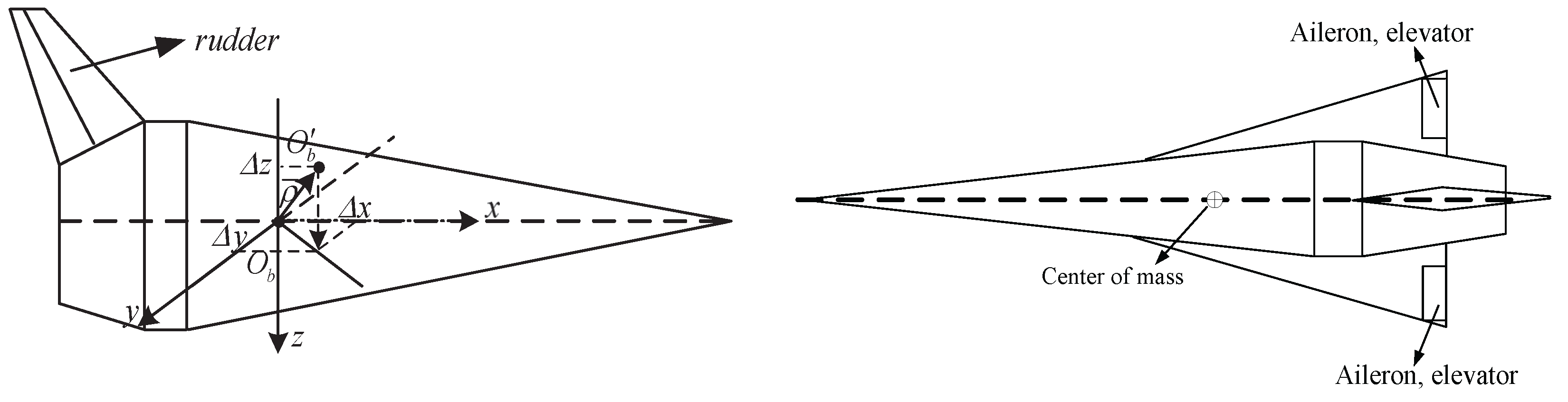
In order to study the effect of an unexpected centroid shift on the motion of the HSV’s attitude system, a detailed study with respect to HSV attitude dynamics with unexpected centroid shift is presented, where the centroid shift refers to the phenomenon that HSV’s original centroid () moves to the current position (), as shown in Figure 1. Based on previous studies [7,9,25], the effect of the unexpected centroid shift can be transmitted in the following two affine subsystems: (1) attitude angle system and (2) attitude angular rate system.
2.1.1. Attitude Angles Affine Nonlinear Equations of HSV with Centroid Shift
According to [8,25], the attitude angle subsystem of HSV with unexpected centroid shift can be developed as:
where V is the velocity vector of the system and represents the flight path angle. and are the attack angle, sideslip angle and roll angle, respectively, and stands for the attitude angular rate vector that consists of rolling rate (p), pitching rate (q) and yawing rate (r). L and Y are the lift and side force of HSV. As for the influences of unexpected centroid shift, , denotes the variation of the center-of-mass location () with respect to the original centroid (, as shown in Figure 1). Moreover, are intermediate variables, shown in (A1), and and are the angular velocities in view of flight-path coordinate frame with respect to the earth-surface inertial coordinate frame, provided in (A2). and are the functions of and , standing for the influence of centroid shift on the system of HSV, seen in (A3). Finally, m is the mass of HSV.
In what follows, in order to facilitate the subsequent theoretical analysis, based on (1)–(3), the affine attitude angle subsystem of HSV is obtained as
where is defined to describe the attitude angle vector. denotes the system matrix, and represents the uncertainty of . In addition, is the tracking index vector of attitude angular rate based on attitude angle tracking error. F stands for the fault factor of the slow-loop controller and the details are seen in (5), which represents a kind of signal gain fault [16]. denotes the influence of centroid shift, external disturbance and virtual controller gain fault of slow-loop of HSV, satisfying that is bounded. The details are described as follows:
T denotes the time of the fault, which occurs at some unknown time. is the signal gain fault of the slow-loop controller, satisfying . When , the output of is in normal condition; while at , the output of is entirely ineffective.
2.1.2. Attitude Angular Rates Affine Nonlinear Equations of HSV with Centroid Shift
In standard aircraft modeling, the mass distribution of an aircraft is assumed to be symmetric with respect to the x–z plane, such that the cross products of the inertial forces and are zero [26]. However, with the unexpected centroid shift ( moving to the original location , as shown in Figure 1), and become nonzero leading to the following moment equations for HSV [7,9,25]:
where and represent the moments of inertia. and are the products of inertia of HSV. In addition, and are the states of HSV with respect to the aircraft body frame, as shown in (A4). For the convenience of theoretical analysis, is introduced as the velocity vector of HSV.
Then, through a close inspection of (6), the affine attitude angular rate subsystem of HSV can be reshaped as
where represents the inertial matrix of HSV, where stands for the inertial matrix without centroid shift and is the uncertainties of inertial matrix due to centroid shift, and the details are explained later. is the external disturbance. Furthermore, is the gravitational force vector.
2.2. Analysis of the Influence of the Centroid Shift on HSV Motion
Before proceeding further, a relative analysis is presented to explain the challenges of this paper. According to previous research about the influence of centroid shift [3,25] and a close inspection of (4) and (7), it can be concluded in the following three aspects: (1) variation of inertial matrix; (2) eccentric moment; and (3) system uncertainty, and the details are delivered as follows:
2.2.1. Variation of Inertial Matrix
As for the , it represents an uncertain portion of J due to the centroid shift (from to , as shown in Figure 1). Details are given as follows:
where the details of are shown as (A5). It is worth pointing out that changes in the inertia matrix of the system (), due to the potential irreversibility of (), will pose challenges to the controller that depends on the inverse matrix of the inertia matrix of the system. Such as in sliding mode control [16], robust adaptive control [27], and so on, resulting in the singularity of the controller or giving rise to the underactuated characteristic of the system. Existing controllers struggle to function properly.
2.2.2. Eccentric Moment
The eccentricity due to the accidental centroid shift is derived as follows
where and are the three components of the system control input vector along the aircraft body frame , as illustrated in Figure 1. The skew symmetric matrix is composed of and and the relative details are displayed as [28]
where D, Y and L are the drag, side force and lift, respectively, which are shown as (A8) and (A9).
2.2.3. The Uncertainty of the System
In contrast to the usual decoupling of system uncertainty from the normal case, by multiplying to both sides of (7), it is obvious that the system uncertainty caused by is difficult to decouple from .
In addition, the remaining part of uncertainty is remarked as [7,8]
where represents the offset vector of the center-of-mass. Furthermore, when , and are non-zero, which means that evolves from the decoupling matrix to the coupling matrix , resulting in a strong coupling between the longitudinal and transverse dynamics of the HSV.
2.3. Actuator Faults
In this work, to describe actuator faults, the control inputs of the system (7) are further modified as [29]
where indicates the designed controller.
Therefore, when , multiple critical and common fault modes can appear as
- Stuck or lock in place (LIP) fault: is a constant, and denotes the disturbance moment;
- Loss of effectiveness (LOE) fault: , with being a positive constant.
2.4. Control Objective
The purpose of this paper is to propose an adaptive compensation-fault-tolerant control scheme that enables the output signal to follow the reference signal without resorting to the exact information of inertia matrix and despite the occurrence of eccentric moments, uncertain system parameters, actuator failures and external disturbances. In addition, signals in a closed-loop system are bounded. To do this, the following assumptions are required.
Assumption 1.
Before and after the occurrence of the unexpected centroid shift, the aerodynamic configuration of the HSV remains the same, that is, there is no variation in the aerodynamic parameters.
Assumption 2.
The inverse of the inertial matrix exists.
Assumption 3.
The complex disturbance satisfies , where is an unknown positive real constant. Besides, the uncertainty of quick-loop system meets , where is an unknown constant, satisfying . The eccentric disturbance moment of HSV satisfies , where is the unknown positive real constant. In addition, the disturbance of quick-loop is also bounded.
Assumption 4.
The desired tracking command signals , and their time-derivative , is continuous and bounded.
Remark 1.
Under Assumption 2, the inertia matrix is an invertible matrix, which plays a crucial role in controller; however, the inverse function of may not exist because is estimated by the estimator. For this challenge, a special negative feedback control is developed in this work without resorting to the exact knowledge of . In addition, based on an auxiliary integrator [30] or necessary gain [31], they can be another way to deal with this problem.
Before the fault-tolerant controller design, a necessary lemma is delivered as follows.
Lemma 1
([32]). The higher-order sliding mode differentiator is defined as
where and are the states of higher-order sliding mode differentiator (13) and is the design parameter. Assisted by the proper parameters, and are true with no input noise after the finite time of the transient process. In addition, the corresponding solution of this dynamic system is Lyapunov stable, i.e., namely finite time stability.
3. Fault-Tolerant Control Design for the Attitude System of HSV
As shown in Figure 2, the fault tolerant control framework with unexpected centroid migration is divided into two prats: slow-Loop control strategy and slow-Loop control strategy. In slow-loop of HSV, the control strategy is consisted of nonlinear generalized predictive control scheme and a high-order sliding mode observer. In fast-loop of HSV, an adaptive feedback fault-tolerant controller that does not need the exact knowledge of is proposed. The details are shown as follows.
3.1. Fault-Tolerant Control Design for Slow-Loop of HSV
To achieve control target, the tracking error vector () of quiet-loop is defined as
where represents the expected index.
3.1.1. Baseline Controller under Nominal Condition
In this work, the nonlinear generalized predictive control, one kind of optimal control is utilized to achieve the control target of the low-loop of HSV due to its excellent dynamic performance [22]. Initially, the receding horizon performance metric was introduced as
where T is the predictive period and represents the predictive tracking error that is defined as
where is the predictive output, and stands for the reference output.
- Obtaining future behaviors. To this aim, by resorting to the Taylor series expansion, the future behavior of can be predicted bywhere , , , , as shown in (A6), where is the relative degree corresponding to the system output, and r is the control order [22]. Then, the index signal is also predicted bywhere , seen in (A6). From this, the tracking error associated with the predicted behavior is derived asMoreover, by some algebraic manipulations and rearrangements of the resulting formulas, the prediction error in the performance index (15) is rewritten asFor analysis purpose, is defined as and its matrix blocks are split by
- Minimizing performance index. In order to minimize the performance index (20) through the proper , the optimal is solved by the following partial differential equation.Based on the assumption that and are reversible, it is obtained thatBy invoking (A6), the front m rows of (24) can be described as followswhere K represents the front m rows of ..Eventually, the optimal control law can be obtained as [33]
Remark 2.
The actual control input , is obtained by the initial value of the optimal control input . Namely, when [22].
Thereafter, a closed inspection of (4) reveals that relative degree , and thus, by keeping (4) and (26) in mind and setting control order , the final baseline controller under nominal condition can be readily designed as
where the unknown complex disturbance of (4) can give rise to the huge challenges for the control performance of the designed controller (27). To deal with such problems, fault-tolerant controllers with the help of observers are utilized in this work, the details of which are communicated in the following sections.
3.1.2. Fault-Tolerant Controller Design under Unexpected Centroid Shift and System Fault
For the adverse effects caused by complex disturbance , as shown in (4), a top-order sliding mode observer is designed in this work to obtain unknown knowledge serving for the basic controller to realize the fault-tolerant control targets.
- High-order sliding mode observer design. To estimate the complex perturbation , a top-order sliding mode observer is designed as follows [21]where and are the designed sliding mode surfaces based on the terminal sliding mode trick, and z denote the state of the designed observer. and are the designed system matrix, satisfying and . In addition, p and q are odd positive integers, satisfying . Furthermore, and are also the designed positive constants to regulate the estimation effect of . Finally, is the estimation of the adaptive parameter .Before analyzing the stability of the disturbance estimate error , combined with (4) and (28), the derivative of is deduced asFurthermore, by keeping the exponential reaching law and (29) in mind, can be obtained asIn what follows, the stability of the designed observer is analyzed through the following Lyapunov functionwhere is a designed parameter, satisfying , and we define that .Evaluating the time derivative of along (28) and (30) leads towhere . Furthermore, invoking , (32) can be further deduced asThe differential term in the designed higher-order sliding-mode observer is not directly obtained by using the derivative method. Moreover, according to Lemma 1, applying a higher-order sliding mode differentiator yields the corresponding derivative. Then, the states z converge to in finite time .
- According to (31), if at time , the states will arrive at the sliding mode in finite time , namelyExamining (34), it is straightforward to show that the sliding mode can be reached within the finite time .
- When the sliding mode is arrived, the convergence time of the system is up to the terminal sliding mode equationwhere denotes a terminal attractor of the system of (35). According to [21], the convergence time from when to when satisfiesIn a similar way, from the time point when move to the time point when , the convergence time is obtained as .
From this, we can obtain that the estimated value be approximated by an external perturbation in finite time . Combined with Assumption 3, we can conclude that the disturbance estimation error is bounded and can be defined as , where is a positive unknown constant. - Fault-tolerant controller design of slow-loop. Recall that Assumption 3, together with the estimate of complex disturbance from observer (28) and the baseline controller (27), the final control law and adaptive law are synthesized aswhere is applied to suppress uncertainties due to unexpected centroid shifts, external perturbations, etc. As for the adaptive term , it is applied to handle the estimation error of , where represents the estimation of .
To analyze the stability of the observer and the resulting closed-loop system, the following theorem summarizes the main results of this subsection.
Theorem 1.
Consider the slow-loop model of HSV describer by (4), with unexpected centroid shift, system fault and disturbance, satisfying Assumptions 1–4, under the designed controller (37) and the observer (28), the slow-loop system of HSV can track expected signals and the whole signals in closed-loop system are bounded.
Proof.
Consider the following Lyapunov function
where is a positive definite symmetric matrix, and is applied to analyze the estimate error of .
Take the derivative of (38) and we have
Therefore, due to the positive definition of , is negative semi-definite, which means is an increasing function of time; that is, the tracking error , and are all bounded. Next, the parameter projection algorithm is applied to modify the adaptive updating laws in both observer and controller to guarantee the boundedness of the designed adaptive parameters . Furthermore, due to , combined with Assumptions 3 and 4, we can infer that is also bounded. Subsequently, based on the Barbalat lemma and the bounded and definition of , it can be obtained that to imply that the slow-loop system of HSV can track expected signals. In this way, Theorem 1 is proved and the argument projection is delivered as follows. □
3.2. Fault-Tolerant Control Design for Fast Loop of HSV
In this part, for the challenges caused by unexpected centroid shift, as shown in (8)–(12), the fault-tolerant controller of the quick-loop is deduced from the three aspects: (1) uncertainties of inertial matrix (J); (2) system uncertainties and eccentric moments; (3) system input saturation.
3.2.1. Fault-Tolerant Controller without Exact Knowledge of Inertial Matrix under Nominal Condition
As for the crucial role of the inertial matrix J on the controller design, once it is unexpectedly moved, as variation () can present great challenges to controllers that rely on the inverse matrix of the system’s inertial matrix due to the potential irreversibility of (), as shown in (8), such as sliding mode control [13], robust adaptive control [27], etc. In order to cope with this question, an adaptive feedback fault-tolerant controller that does not need the exact knowledge of is developed in this work to handle this question.
Before the fault-tolerant controller design, the angular velocity error is introduced as
where is the desired angular velocity. Furthermore, combined with Assumption 4 and (7), taking the derivative of yields [23]
Considering (41) and (42), by assuming that system uncertainty , external disturbance and eccentric moment are all known, the nominal controller without the knowledge of J is developed to achieve that is bounded and the other signals are bounded. The details are conveyed in the following three steps.
- Step 1, a linear operator acting on is introduced byThen, based on (8), an intermediate vector is introduced to obtain the following transformation.
- Step 3, combined with Assumption 2, an adaptive feedback control law and its adaptive law are synthesized aswhere is a designed as positive definite symmetric matric, and represents the designed parameter, satisfying .
3.2.2. Adaptive Fault-Tolerant Controller without Exact Knowledge of Inertial Matrix
Due to the unknown effects of system uncertainty , external disturbance and eccentric moment deriving from unexpected centroid shifts, actuator failures and external disturbances have a huge impact on the control performance of the designed controller (47). In order to overcome this obstacle, based on the characteristics of system uncertainty (11), eccentric moment (9) and LOE fault of actuator (12), the following adaptive laws are designed as
- System uncertainty. By means of the Jacobi identity of the cross product, , where are the vectors. In view of (11), we havewhere , remarked as . From this it follows thatSubsequently, its adaptation law was developed aswhere is a designed adaptive variable to estimate the unexpected effects of system uncertainties caused by centroid shift. Further, represents a designed positive definite symmetric parameter matrix, and stands for a constant coefficient, satisfying .
- Eccentric moment. For clarity, the effect of the eccentricity moment is rewritten as follows.and the corresponding adaptation law is developed aswhere is also an adaptive state to obtain the effect of the eccentricity moment. represents a design with positive definite symmetric coefficient matrix, and is also a positive parameter.
- LOE fault of actuator and external disturbance. For actuator faults and external perturbations , the complex perturbation is defined aswhere stands for the failure factor of the actuator fault, as shown in (12). Furthermore, combined with Assumption 3, the bounds of are introduced as , satisfying , where . Furthermore, an adaptive estimator is introduced aswhere is also utilized to estimate the influence of disturbance and LOE fault of actuator. and are both positive constants.
In conclusion, combined with (50), (52) and (54), the nominal fault-tolerant controller of quick-loop (47) can be further developed as
Eventually, based on the Lyapunov stability theorem, a theoretical analysis is performed to summarize the main results of this section and guarantee the stability of the closed-loop control system.
Theorem 2.
Considering the quick-loop dynamics of a hypersonic vehicle (7) suffered from the variation of inertial matrix (8), eccentric moment (9), system uncertainty (11), actuator failures (12) and external disturbances, , adaptive feedback controls (55) without resorting to the exact knowledge of inertial matrix J by means of the adaptive laws (50), (52) and (54) developed to ensure that the quick-loop system of HSV can track expected signals, converging to a tiny compact set of the origin, and all the closed signals are bounded.
Proof.
First, let us choose a positive definite Lyapunov function candidate as
where the estimate errors of , and are defined as .
Subsequently, by taking the following inequalities
into consideration, (58) can be further deduced as
Furthermore, two indirect designed parameters are adopted as
Finally, (60) is reshaped as
By multiplying into both sides of (62) and integrating at the interval , we have
where is the initial actuation time and .
Furthermore, by defining that , combined with the definition of in (56), the boundedness of attitude angle rate error can be obtained as
where is the minimum eigenvalue of inertia matrix J. Moreover, note that as . As a result, .
In addition, to guarantee the boundedness of the system parameters, the adaptive update law is modified by the parameter projection algorithm. The compact sets , , and are defined to restrain the above adaptive laws and the details are shown as follows [19]
where , , , and , , , are the lower and upper bounds of adaptive laws. Then, the adaptive laws of , , and are modified as follows
where
Finally, since by assumption and are bounded, it can be obtained that is bounded as well. Since the boundedness of is already guaranteed by the use of the parametric projection operator, the stability of the closed-loop system is ensured and all the signals of the HSV fast-loop are bounded. □
4. Simulation
Considering that the HSV is carrying out a hypersonic re-entry flight with the speed of , there is an altitude of and a mass of kg. The initial altitude vector is and the angular rate is . The reference signals are set as during 1 s~8 s, during 8 s∼20 s and during s, besides, is always and is keeping . In addition, the loss of efficiency fault of the actuator was set to as the 5th second.
The external perturbations of low-loop and quick-loop systems of HSV are described as follows , , , , . The design parameters of the low-loop controller of HSV are as follows , . , , , . As for the fast-loop controller, , , .
To study the effect of the centroid shift on the HSV motion and validate the effectiveness of the designed fault-tolerant controller, simulations were performed. For analyzing the effects of unexpected centroid shift on the longitudinal movement of HSV, compared with the tracking effects of the FTC strategy consisted of sliding mode control combined with nonlinear disturbance observer and the FTC controller based on RBFNN [10], the simulation results demonstrate the effectiveness of the designed FTC strategy.
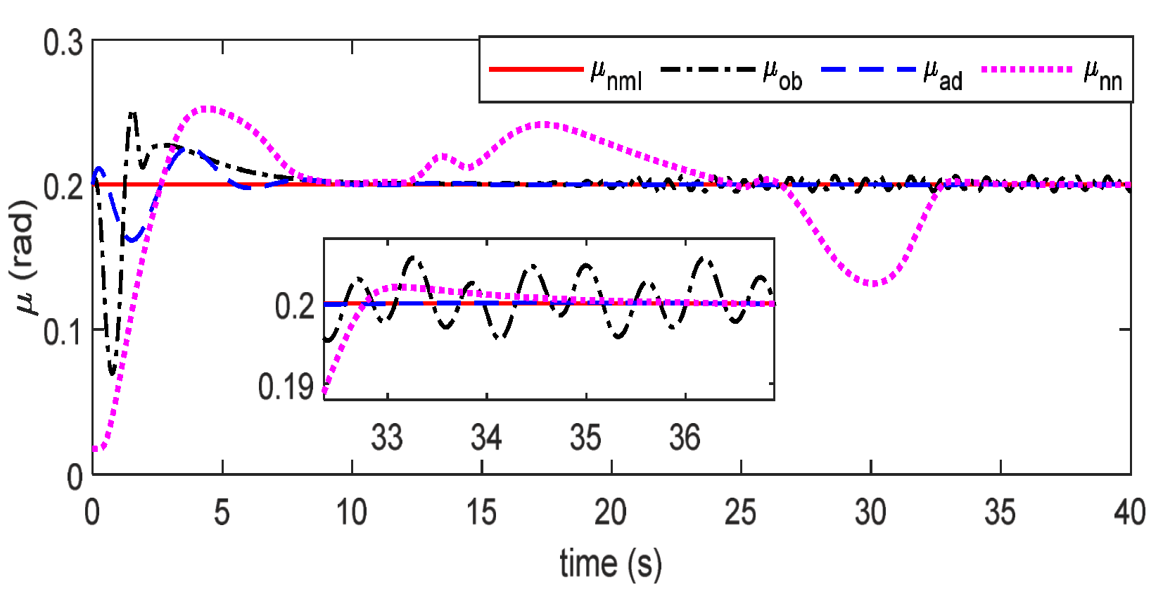
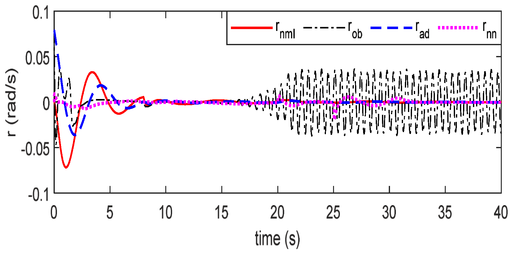
As shown in Figure 3, Figure 4, Figure 5, Figure 6, Figure 7, Figure 8, Figure 9, Figure 10 and Figure 11, is the expected index of HSV’s slow and fast loops. represents the fault-tolerant control effect of sliding mode controller (SMC) combined with the nonlinear disturbance observer (NDO) [35] by moving the uncertainties of on the right hands of attitude dynamics, and represents the simulation results of a control scheme that is composed of nonlinear generalized predictive control (NGPC) and radial basis function neural network (RBFNN), as shown in [10]. In addition, denotes the control effect of the controller designed in this paper. On the basis of Figure 3, Figure 4, Figure 5, Figure 6, Figure 7 and Figure 8, in case of actuator failure only at the fifth second, attitude angles () with and tracking effect, has faster convergence speed. The main reason may be the heavy line load calculation of RBFNN and the horizontal regression principle of NGPC. Before the centroid shift occurs, it is straightforward to verify that the above controller presents an acceptable FTC tracking effect based on the arguments above.
When the unforeseeable centroid displacement occurs in the second, the eccentric movement and variation of inertial matrix combined with the LOE fault of the actuator give rise to the fluctuation of the control surface of compared with that of and , as shown in Figure 9, Figure 10 and Figure 11. However, this does not affect the steady flight of the HSV considerably for the time being, as shown by the trajectories in Figure 3, Figure 4, Figure 5, Figure 6, Figure 7 and Figure 8 during the 10th and 20th seconds. Once the attitude angle index of HSV changes in the second, found in Figure 3, Figure 4, Figure 5, Figure 6, Figure 7 and Figure 8, the attitude angles and attitude angular rates both exhibit the phenomenon of rapid fluctuation in compared with that of . Besides, the tracking effects of are of high tracking accuracy, but the relative low convergence speed, for instance, the tracking effect of of Figure 3. It can be concluded that when the centroid shift and actuator fault both occur, the usual control strategy consisted of sliding mode controller and NDO can not work well under the variation of the inertial matrix J caused by unexpected centroid shift, which needs a more stable system control structure (exact knowledge of J and ), but the FTC strategies of and do not need.
Figure 9.
Control surface deflection angles of .

Figure 10.
Control surface deflection angles of .

Figure 11.
Control surface deflection angles of .

Furthermore, due to unknown effects being integrated into one item to facilitate the observation of NDO, the larger deflection angles of control surfaces are needed to cope with the estimated effects through NDO, as shown in the response curves of control surfaces of Figure 9, Figure 10 and Figure 11 after the 20th second. Moreover, given the heavy online computational load of neural networks, the application of FTC controller resting on RBFNN is utilized to handle effects (, and ) one-by-one obtain excellent tracking effects, but this FTC scheme shows a low convergence speed, shown in the tracking effects of in Figure 9, Figure 10 and Figure 11. To remedy this, the FTC algorithm of this work is developed by employing adaptive observers and estimators in conjunction with adaptive feedback control, which has a known and fixed control structure and does not need the exact knowledge of inertial matrix (J and ). Finally, the simulation results show that the proposed FTC strategy in this work can suppress unexpected effects and maintain excellent tracking performance.
5. Conclusions
In this paper, we develop a useful solution to the HSV problem with unexpected centroid shifts, actuator faults and external perturbations. Resorting to a designed sixth-order dynamic compensator, the proposed adaptive FTC scheme can achieve the attitude tracking objective without the exact knowledge of the inertia matrix J, despite the presence of variations in the system inertia matrix, eccentricity and actuator faults. Subsequently, based on the properties of eccentric moments, systematic uncertainties and external perturbations, the performance of the proposed FTC controller can be improved by adapting the corresponding adaptive estimator to support the designed FTC controller using adaptive techniques.Then, the stability of this designed FTC strategy is guaranteed by the Lyapunov stability theorem. Finally, the simulation results show that the proposed FTC scheme is effective for the reconfigurable HSV flight control design under the condition of the inertia matrix and eccentricity.
In future work, we will focus on the FTC of HSV with structural failures caused by variable centroid displacement (the structure and size of the elements of the inertial matrix J are uncertain). Furthermore, the problem of deflection saturation of the control surface should also be taken into consideration [24].
Author Contributions
Writing—original draft preparation, H.Y.; writing—review and editing, Y.M. All authors have read and agreed to the published version of the manuscript.
Funding
This work was supported by the National Natural Science Foundation of China (61773012), the National natural sciences fund youth fund project (61807017), the research start-up fund of Jiangsu University of science and technology (1052932101).
Institutional Review Board Statement
This study did not involve humans or animals.
Informed Consent Statement
This study did not involve humans or animals.
Data Availability Statement
Conflicts of Interest
The authors declare that they have no known competing financial interests or personal relationships that could have appeared to influence the work reported in this paper.
Appendix A
Appendix B
and Y are described as follows [33]
where . , , and . and are the control deflections of the aileron, elevator and rudder, respectively.
The rolling, pitching and yawing moments are described as [28]
where , , . ,
References
- Tang, T.; Qi, R.Y.; Jiang, B. Adaptive nonlinear generalized predictive control for hypersonic vehicle with unknown parameters and control constraints. Proc. Inst. Mech. Eng. Part G J. Aerosp. Eng. 2017, 233, 510–532. [Google Scholar] [CrossRef]
- Yu, X.; Li, P.; Zhang, Y.M. The design of fixed-Time observer and finite-time fault-tolerant control for hypersonic gliding vehicles. IEEE Trans. Ind. Electron. 2018, 65, 4135–4144. [Google Scholar] [CrossRef] [Green Version]
- Nguyen, N.; Krishnakumar, K.; Kaneshige, J.; Nespeca, P. Dynamics and adaptive control for stability recovery of damaged asymmetric aircraft. In Proceedings of the AIAA Guidance, Navigation, and Control Conference and Exhibit, Keystone, CO, USA, 21 August 2006; p. 6049. [Google Scholar]
- Li, J.; Gao, C.; Jing, W.; Wei, P. Dynamic analysis and control of novel moving mass flight vehicle. Acta Astronaut. 2017, 131, 36–44. [Google Scholar] [CrossRef]
- Li, J.Q.; Gao, C.S.; Li, C.Y. A survey on moving mass control technology. Aerosp. Sci. Technol. 2018, 82, 594–606. [Google Scholar] [CrossRef]
- Gasbarri, P.; Sabatini, M.; Pisculli, A. Dynamic modelling and stability parametric analysis of a flexible spacecraft with fuel slosh. Acta Astronaut. 2016, 127, 141–159. [Google Scholar] [CrossRef]
- Bacon, B.J.; Gregory, I.M. General equations of motion for a damaged asymmetric aircraft. AIAA Paper 2007-6306. In Proceedings of the 2007 AIAA Guidance, Navigation, and Control Conference, Hilton Head, SC, USA, 20 August 2007. [Google Scholar]
- Nguyen, N.; Krishnakumar, K.; Kaneshige, J.; Nespeca, P. Flight dynamics modeling and hybrid adaptive control of damaged asymmetric aircraft. J. Guid. Control. Dyn. 2008, 31, 171–186. [Google Scholar]
- Liu, Y.; Tao, G.; Joshi, S.M. Modeling and model reference adaptive control of aircraft with asymmetric damage. J. Guid. Control. Dyn. 2012, 33, 1500–1517. [Google Scholar] [CrossRef]
- Meng, Y.Z.; Jiang, B.; Qi, R.Y. Adaptive non-singular fault-tolerant control for hypersonic vehicle with unexpected centroid shift. IET Control Theory Appl. 2019, 13, 1773–1785. [Google Scholar] [CrossRef]
- Lee, T. Robust adaptive attitude tracking on SO(3) with an application to a quadrotor UAV. J. Guid. Control. Dyn. 2013, 21, 1924–1930. [Google Scholar]
- Yin, S.; Ding, S.X.; Xie, X.; Luo, H. A review on basic data-driven approaches for industrial process monitoring. IEEE Trans. Ind. Electron. 2014, 61, 6418–6428. [Google Scholar] [CrossRef]
- Xiao, B.; Yin, S.; Hao, H. Reconfigurable tolerant control of uncertain mechanical systems with actuator faults: A sliding mode observer-based approach. IEEE Trans. Control Syst. Technol. 2018, 26, 1249–1258. [Google Scholar] [CrossRef]
- Bounemeur, A.; Chemachema, M.; Essounbouli, N. Indirect adaptive fuzzy fault-tolerant tracking control for MIMO nonlinear systems with actuator and sensor failures. ISA Trans. 2018, 79, 45–61. [Google Scholar] [CrossRef] [PubMed]
- Hu, Q.; Niu, G.; Wang, C. Spacecraft attitude fault-tolerant control based on iterative learning observer and control allocation. Aerosp. Sci. Technol. 2018, 75, 245–253. [Google Scholar] [CrossRef]
- Xu, D.Z.; Jiang, B.; Shi, P. Robust NSV fault-tolerant control system design against actuator faults and control surface damage under actuator dynamics. IEEE Trans. Ind. Electron. 2015, 62, 5919–5928. [Google Scholar] [CrossRef]
- Jiang, B.; Gao, Z.; Shi, P.; Xu, Y. Adaptive fault-tolerant tracking control of near-space vehicle using takagi-sugeno fuzzy models. IEEE Trans. Fuzzy Syst. 2010, 18, 1000–1007. [Google Scholar] [CrossRef]
- Yin, S.; Yang, H.; Gao, H.; Qiu, J.; Kaynak, O. An adaptive NN-based approach for fault-tolerant control of nonlinear time-varying delay systems with unmodeled dynamics. IEEE Trans. Neural Netw. Learn. Syst. 2017, 28, 1902–1913. [Google Scholar] [CrossRef]
- He, J.; Qi, R.; Jiang, B.; Qian, J. Adaptive output feedback fault-tolerant control design for hypersonic flight vehicles. J. Frankl. Inst. 2015, 352, 1811–1835. [Google Scholar] [CrossRef]
- Zhang, A.; Hu, Q.L.; Friswell, M.I. Finite-time fault tolerant attitude control for over-activated spacecraft subject to actuator misalignment and faults. Iet Control Theory Appl. 2013, 7, 2007–2020. [Google Scholar] [CrossRef] [Green Version]
- Chen, M.; Yu, J. Disturbance observer-based adaptive sliding mode control for near-space vehicles. Nonlinear Dyn. 2015, 82, 1671–1682. [Google Scholar] [CrossRef]
- Chen, W.H.; Ballance, D.J.; Gawthrop, P.J. Brief optimal control of nonlinear systems: A predictive control approach. Automatica 2003, 39, 633–641. [Google Scholar] [CrossRef] [Green Version]
- Chaturvedi, N.A.; Bernstein, D.S.; Ahmed, J.; Bacconi, F.; McClamroch, N.H. Globally convergent adaptive tracking of angular velocity and inertia identification for a 3-DOF rigid body. IEEE Trans. Control. Syst. Technol. 2006, 14, 841–853. [Google Scholar] [CrossRef] [Green Version]
- Hu, Q.; Shao, X.; Guo, L. Adaptive fault-tolerant attitude tracking control of spacecraft with prescribed performance. IEEE/ASME Trans. Mechatron. 2018, 23, 331–341. [Google Scholar] [CrossRef]
- Meng, Y.Z.; Jiang, B.; Qi, R.Y. Modeling and control of hypersonic vehicle dynamic under centroid shift. Adv. Mech. Eng. 2018, 10, 1–21. [Google Scholar] [CrossRef]
- Zong, Q.; Zeng, F.L.; Zhang, B.X.; You, M. Modeling and Model Verification of Hypersonic Vehicle; Science China Press: Beijing, China, 2016. [Google Scholar]
- Yang, H.; Jiang, B.; Liu, H.H.; Yang, H.; Zhang, Q. Attitude synchronization for multiple 3-DOF helicopters with actuator faults. IEEE/ASME Trans. Mechatron. 2019, 24, 597–608. [Google Scholar] [CrossRef]
- Shaughnessy, J.D.; Pinckney, S.Z.; McMinn, J.D. Hypersonic Vehicle Simulation Model: Winged-Cone Configuration; NASA TM-102610; NASA Langley Reserch Center: Hamption, VA, USA, 1990; pp. 1–140.
- Xu, B.; Qi, R.; Jiang, B. Adaptive fault-tolerant control for HSV with unknown control direction. IEEE Trans. Aerosp. Electron. Syst. 2019, 55, 2743–2758. [Google Scholar] [CrossRef]
- Liu, Y.H.; Huang, L.; Xiao, D. Adaptive dynamic surface control for uncertain nonaffine nonlinear systems. Int. J. Robust Nonlinear Control 2017, 27, 535–546. [Google Scholar] [CrossRef]
- Xian, B.; Zhang, Y. Continuous asymptotically tracking control for a class of nonaffine-in-input system with non-vanishing disturbance. IEEE Trans. Autom. Control 2017, 62, 6019–6025. [Google Scholar] [CrossRef]
- Levant, A. Higher-order sliding modes, differentiation and output-feedback control. Int. J. Control 2003, 76, 924–941. [Google Scholar] [CrossRef]
- Du, Y.L. Study of Nonlinear Adaptive Attitude and Trajectory Control for Near Space Vehicles; Nanjing University of Aeronautics and Astronautics: Nanjing, China, 2010. [Google Scholar]
- Lai, G.; Liu, Z.; Zhang, Y.; Chen, C.P. Adaptive position/attitude tracking control of aerial robot with unknown inertial matrix based on a new robust neural identifier. IEEE Trans. Neural Netw. Learn. Syst. 2016, 27, 18–31. [Google Scholar] [CrossRef]
- Lee, D. Nonlinear disturbance observer-based robust control for spacecraft formation flying. Aerosp. Sci. Technol. 2018, 76, 82–90. [Google Scholar] [CrossRef]
Figure 1.
Three-dimensional view of the displacement of the center of mass, .

Figure 2.
Frame of fault-tolerant controller for HSV with centroid shift.

Figure 3.
Tracking effects of attack angle .

Figure 4.
Tracking effects of bank angle .

Figure 5.
Tracking effects of sideslip angle .

Figure 6.
Tracking effects of roll rate p.

Figure 7.
Tracking effects of pitch rate q.

Figure 8.
Tracking effects of yaw rate r.

Disclaimer/Publisher’s Note: The statements, opinions and data contained in all publications are solely those of the individual author(s) and contributor(s) and not of MDPI and/or the editor(s). MDPI and/or the editor(s) disclaim responsibility for any injury to people or property resulting from any ideas, methods, instructions or products referred to in the content. |
© 2023 by the authors. Licensee MDPI, Basel, Switzerland. This article is an open access article distributed under the terms and conditions of the Creative Commons Attribution (CC BY) license (https://creativecommons.org/licenses/by/4.0/).
Share and Cite
MDPI and ACS Style
Ye, H.; Meng, Y. Adaptive Fault-Tolerant Control of Hypersonic Vehicles with Unknown Model Inertia Matrix and System Induced by Centroid Shift. Appl. Sci. 2023, 13, 830. https://0-doi-org.brum.beds.ac.uk/10.3390/app13020830
AMA Style
Ye H, Meng Y. Adaptive Fault-Tolerant Control of Hypersonic Vehicles with Unknown Model Inertia Matrix and System Induced by Centroid Shift. Applied Sciences. 2023; 13(2):830. https://0-doi-org.brum.beds.ac.uk/10.3390/app13020830
Chicago/Turabian StyleYe, Hui, and Yizhen Meng. 2023. "Adaptive Fault-Tolerant Control of Hypersonic Vehicles with Unknown Model Inertia Matrix and System Induced by Centroid Shift" Applied Sciences 13, no. 2: 830. https://0-doi-org.brum.beds.ac.uk/10.3390/app13020830
Note that from the first issue of 2016, this journal uses article numbers instead of page numbers. See further details here.