
Wind Speed Spectrum of a Moving Vehicle under Turbulent Crosswinds


School of Civil Engineering and Architecture, Southwest University of Science and Technology, Mianyang 621010, China
Appl. Sci. 2023, 13(21), 12054; https://0-doi-org.brum.beds.ac.uk/10.3390/app132112054
Submission received: 13 September 2023
/
Revised: 25 October 2023
/
Accepted: 3 November 2023
/
Published: 5 November 2023
Abstract
:Wind loads have become one of the key influencing factors for the running safety of vehicles and comfort of passengers. The investigation of the wind speed spectrum characteristics of a moving vehicle under turbulent crosswinds is of great importance. Expressions of the wind speed spectrum of a moving vehicle were obtained from the von Kármán spectrum, based on Taylor’s frozen flow hypothesis. The influencing factors, including the ratio of the vehicle speed to the wind speed and wind yaw angles, were analyzed. The change rules of the wind speed spectrum peak and its corresponding frequency were also studied. The results show that the wind speed spectrum peak values of the moving vehicle were larger than those of the static vehicle. The wind speed spectrum peak values corresponding to the moving vehicle were first increased and then decreased, as the wind yaw angles increased. Some of the frequencies corresponding to the longitudinal wind speed spectrum values of the moving vehicle were smaller than those of the static vehicle. Therefore, the energy had been transferred to the lower frequency. For the moving vehicle, the frequency values corresponding to the longitudinal wind speed spectrum peak were first increased and then decreased, as the ratio of the vehicle speed to the wind speed and the wind yaw angle increased.
1. Introduction
The influence of crosswinds on a moving vehicle deserves constant attention. Severe wind disasters may influence the moving-speed limit of a vehicle, affect its transportation capacity, and even cause vehicle shutdown or accidents [1,2,3,4,5]. For example, China is one of the few countries in the world that is prone to severe wind disasters. In 2007, when the Lanzhou–Xinjiang Line crossed the Gobi gale area in Xinjiang, China, a train vehicle was derailed by strong winds. There were 11 cars overturned and the line was interrupted for nine hours. On 24 February 2008, 48 Japanese trains were stopped, and 183 trains were delayed due to a serious wind disaster which affected about 140,000 people. Meanwhile, the wind has caused train vehicles to be late in some conditions.
Wind loads have become one of the key influencing factors on the coupling vibration of wind–vehicle–bridge systems, which could help to evaluate the running safety and comfort effectively. Mostly, the vehicles run on girders and the wind load’s influence on aerodynamic characteristic should be studied. The wind speed spectrum of a moving train plays a crucial role in examining the wind load characteristics of the train vehicle. The investigation into moving trains carries considerable engineering implications. The aerodynamic characteristics of static vehicles under crosswinds has been experimentally investigated considering the aerodynamic coupling effect between the train vehicle and a bridge [6,7,8]. Investigation of the wind speed spectrum is relatively rare.
Originally, the total wind speed of a moving vehicle was obtained based on that of the static point from the traditional wind field simulation method. The wind flow field is artificially divided into several relevant wind speed intervals along the vehicle’s moving direction. As the wind field mutational effect would occur and leads to deviation in the calculation results which is inconsistent with the actual situation [9,10], investigation of the wind speed spectrum of a moving point that is consistent with the actual situation is of great significance.
Many scholars have studied the characteristics of the wind speed spectra of moving train vehicles. Cooper [11] theoretically derived the longitudinal wind speed spectrum of a moving vehicle. However, the derivation only targets the working conditions in which the angle between the wind speed and the train vehicle’s moving direction is 90°, which could not be widely applied. Obviously the wind yaw angle is varied, so the corresponding working conditions should be studied.
The on-road turbulent wind environment has been measured utilizing a vehicle instrumented with mast-mounted cross wire and propeller-vane anemometers [12,13]. In the conditions of the vehicle’s moving speed at 27.8 m/s and the wind speed at 1–9 m/s, the measured longitudinal and lateral turbulence intensities of the moving point were 2.5~5% and 2~10%, respectively. This could also be obtained numerically, and the study of the wind speed spectrum of a moving point can provide the basis for analyzing wind speed time series and turbulence intensity.
Hu [14,15] developed another analytical model of the wind speed spectrum. Based on the wind speed time series, Yu [16] computed the unsteady aerodynamic load on a moving vehicle. However, the difference between the wind spectra of the static and moving points was not compared comprehensively. For example, the influence of wind yaw angles from 0°~180° was not investigated widely.
Wu [17] numerically studied the correlation characteristics of a moving vehicle preliminarily. This was only studied for a smaller vehicle’s moving speed and the influence of the vehicle’s moving speed was not calculated roughly. Li and Su [18] experimentally investigated the wind spectrum of a moving point under crosswinds in a wind tunnel. The results were compared to those of Balzer’s [19] and Cooper’s models [11], while the cross-correlation characteristics of two moving points were not investigated. The cross-correlation characteristics of two moving points has not yet been extensively explored, which is an important part in the investigation of the wind speed spectrum of a moving point.
Study of the wind speed spectrum characteristics of a moving vehicle and its mathematical model is conducted in this manuscript. An analytical expression of the wind speed spectrum was firstly deduced in a new analytical model. The influence of the wind yaw angle, and the ratios of the wind speed to vehicle moving speed were then fully discussed. Thirdly, the cross-correlation characteristics of two moving points are studied. This could provide a parameter basis for the analysis of wind loads on moving trains.
2. Wind Speed Spectrum Models
2.1. Wind Speed Spectrum of a Static Vehicle
The correlation characteristics of two points in a turbulent flow field can be expressed in terms of the correlation functions f(r) and g(r), where f(r) is the cross-correlation function of the wind speeds for two points apart from r along the axis of the two points (Figure 1a), and g(r) is the cross-correlation function of two points apart from r which are perpendicular to the axis (see Figure 1b) [20].
where u1, u2 and u3 are the fluctuating wind speeds in the x, y and z directions, at time t, for a point in the spatial turbulent flow field, respectively. x, y and z directions are the longitudinal, lateral and vertical directions.
The longitudinal (S11(k1)) and lateral (S22(k1)) wind speed spectra can be obtained by the two following formulas [20]:
where and are the root mean squares of the fluctuating wind speeds in the longitudinal and lateral directions, , ; , , f is the frequency value and U is the incoming mean wind speed.
Von Kármán [20] derived the relationship between g(r) and f(r) based on the spherical symmetry assumption.
Bullen [21] derived the mathematical models of the main correlation functions based on the isotropic turbulence theory:
where a and n are the parameters controlling the shape and scale, respectively; Kn and Kn−1 are the second type of Bessel function; and Γ is the Gamma function.
In the isotropic turbulence field, the relationship [20] between the turbulence integral scale L and the parameter a is satisfied as follows:
Respectively inserting Equations (6) and (7) into Equations (3) and (4) yields
2.2. Wind Speed Spectrum of a Moving Vehicle
Figure 2 shows two points (Points P and P’) fixed on a vehicle and the corresponding equivalent points.
The wind speed is . The moving vehicle travels at a constant speed VT along the straight line ON, which passes through the origin of the overall coordinate system O-XYZ. The angle between the line ON and the x-axis is , which is the wind yaw angle. The overall coordinate system is fixed to the ground and the moving coordinate system N-ξηζ is fixed to the moving vehicle. The η-axis is the moving direction of the vehicle, and the ζ-axis is parallel to the z axis. Points P and P′ are the fixed points on the moving vehicle, whose coordinates in the local coordinate system N-ξηζ are (0, η, ζ) and (0, η′, ζ′), respectively. In the overall coordinate system O-XYZ, the position vector of point P at t and t + τ moments could be accessible.
The time delay can be transformed into an equivalent spatial interval according to Taylor’s freezing hypothesis. Thus, for the physical point P’ (at time t + τ), there are corresponding equivalent points in the frozen turbulent flow field (at time t). The cross-correlation characteristics between point P and P′ that move with the vehicles could be equivalent to the cross-correlation between point P and points in the frozen turbulent flow field.
In the frozen turbulent flow field, the equivalent interval between point P and points could be the projected distances on the x axis, y axis and z axis, respectively:
where is the mean wind speed of the incoming flow.
The cross-correlation function between the two points on a moving vehicle could be expressed as follows:
where , ; , , , = 0.747 and · .
and is the longitudinal integral scale in x, y and z direction.
When point P and point P′ coincide, Equation (13) becomes as follows:
where , .
In the turbulent flow field, the turbulent power spectral density function of a single moving point can be obtained from the autocorrelation function by Fourier transform.
where is the root mean square of the fluctuating wind speed in the longitudinal direction.
According to and , thus:
where . is the root mean square of the fluctuating wind speed in the lateral direction.
When Equation (17) and Equation (18) are put into Equation (16), Equation (16) becomes as follows:
For the von Kármán wind spectrum, = 0.747.
The parameter values of the power spectral density function of a moving point are as follows:
When the wind speed spectrum at a static point is the von Kármán wind spectrum, the corresponding wind spectrum of a moving point can be obtained.
where .
Therefore, based on the theoretical derivation process of the wind velocity spectrum of a static point and the corresponding moving point, a general equation of the wind speed spectrum for a moving point can be obtained. For the von Kármán wind speed spectrum of a static point, the corresponding wind speed spectrum of a moving point can be obtained. The derivation process of the transverse wind velocity spectrum at the moving point is similar to that of the longitudinal wind velocity spectrum. The difference is mainly related to ci (i = u, v), Lu and VR. In this study, the investigation mainly focuses on the longitudinal wind velocity spectrum of a moving point.
2.3. Validation of the Proposed Model
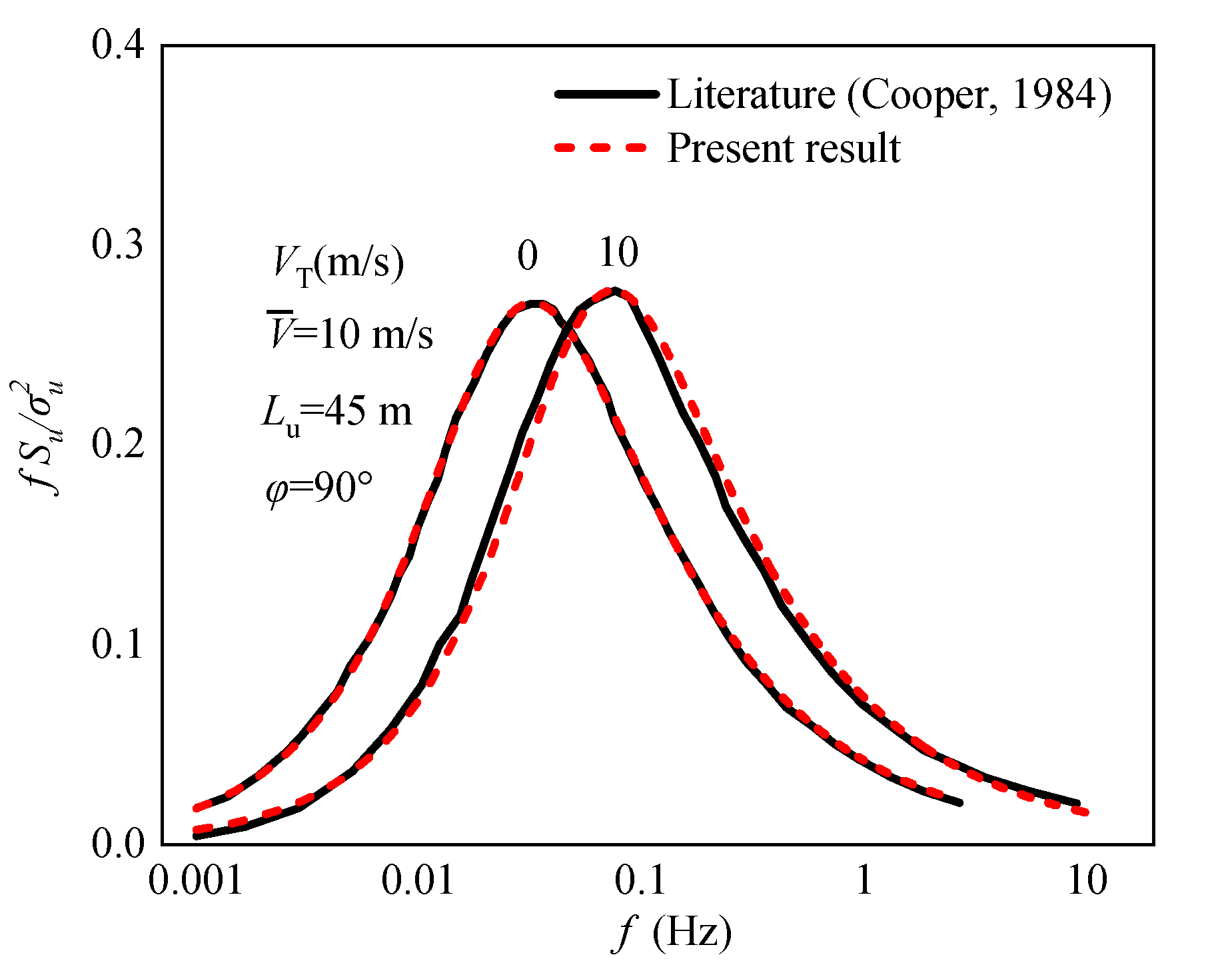
To verify the validation of the derivation process, Figure 3 shows the comparison curve of Cooper’s results and the results derived in Section 2.2. The train vehicle’s moving velocity is 0 m/s and 10 m/s and the longitudinal turbulence integral scale is 45 m. The incoming wind flow is perpendicular to the moving direction of the train vehicle. In Figure 3, the horizontal axis coordinates are in log form. It is known that the derived results align well with Cooper’s results, which verifies that the derivation procedure presented in this paper is accurate.
3. Turbulent Wind Flow Characteristics in Wind Tunnel
3.1. Wind Tunnel Tests
The experimental process was conducted at the XNJD-3 wind tunnel located at Southwest Jiaotong University in China, and the wind tunnel is currently the world’s largest boundary layer wind tunnel. The atmospheric boundary layer flows were produced using a combination of spires and cubes. The setup covers roughly 25 m of the floor of the wind tunnel.
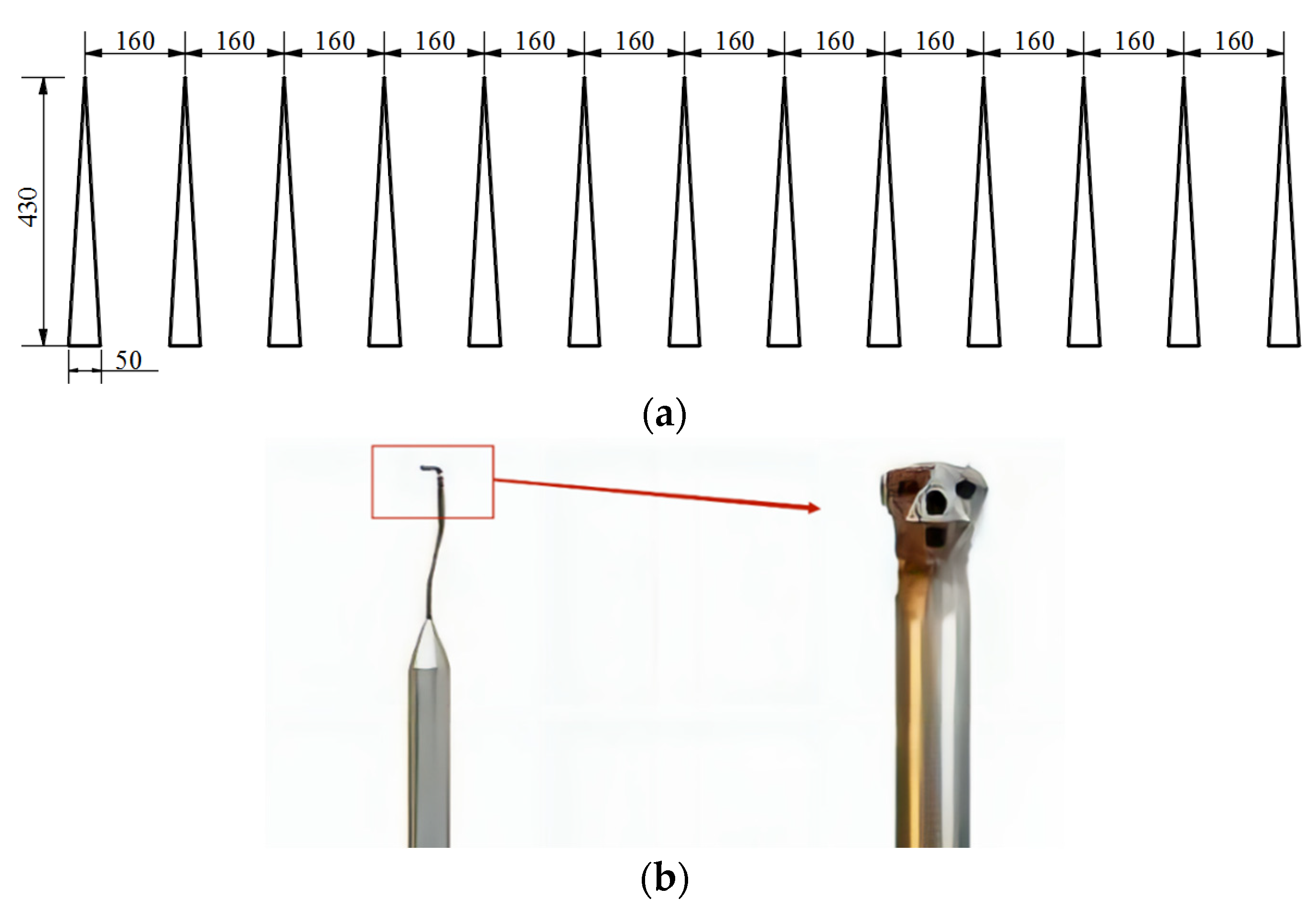
One typical form of atmospheric boundary layer flow is simulated in this study. The turbulent wind field was generated using 13 rectangular spires with a distance interval of 0.16 m (Figure 4). The wind characteristics of the simulated flows were measured by a Cobra probe (Turbulent Flow Instrument series 100). The sampling frequency was set to 256 Hz and the sampling time was 180 s. The Cobra Probe was placed in the middle of wind tunnel in the width direction. The mean and turbulent wind characteristics along the horizontal direction were basically consistent.
3.2. Turbulent Wind Flow Characteristics
Table 1 tabulates the values of the turbulence intensity and integral length scales. Figure 5 shows the comparison between the normalized stream-wise longitudinal velocity power spectral density (PSD) measured in mean turbulence conditions and the interpolation of the real-wind-normalized PSD provided by von Kármán as a function of the reduced frequency. The curves in Figure 5 align well.
4. Wind Speed Spectrum of a Moving Vehicle
4.1. Results
By putting the parameter results from Table 1 into Equation (23), the wind speed spectrum of a moving point can be obtained. Figure 6 shows the spectrum results of a moving point corresponding to the static point in the wind tunnel simulated turbulence field at a wind yaw angle of 15°~175° for 12 total working conditions. In Figure 6, VT is the vehicle’s moving speed, is the incoming wind speed and is the wind yaw angle. Vratio represents the ratio between the vehicle’s moving speed VT and the incoming wind speed . When the vehicle’s moving speed is zero, it is the wind speed spectrum of the static point corresponding to the spire’s turbulent flow field in the wind tunnel tests. The turbulent integral scale adopts the results of Table 1. The main results are shown in Figure 6.
The ratios of the vehicle’s moving speed to the incoming wind speeds are 0~5. If the train vehicle’s moving speed is 200 km/h and the wind speed is 11 m/s, the Vratio value can reach 5. For a moving car on highway, the moving speed is 120 km/h and the wind speed is 11 m/s, so the Vratio value is about 3.3. The once-in-a-century wind speed in mountainous areas can reach 30 m/s or higher. The ratio of the vehicle’s moving speed to the wind speed is thus approximately 2. Therefore, ratios of 0~5 are considered in this investigation.
As can be seen in Figure 6, the basic shape of the wind velocity spectrum varies little. The main differences are found at the wind speed spectrum peaks and the corresponding frequencies.
When the Vratio =1 and the wind yaw angle = 15°, the wind speed spectrum peak is the same as that of the static point, while the frequency corresponding to the peak is larger than that of the static point. The wind speed spectrum peak of the moving point gradually becomes larger than that of the static point. As the wind yaw angle increases, the wind velocity spectrum peak and the corresponding frequency of the moving point also gradually increase. At different wind yaw angles, the wind speed spectrum peak of the moving point gradually moves to higher frequencies.
When the wind yaw angle is 15°~45°, the peak wind speed spectrum values of the moving point remain unchanged as the Vratio values increase. The wind spectrum peak just corresponds to a larger frequency. When the wind yaw angle is 60°, the peak values and the corresponding frequencies increase as the Vratio value increases. The wind yaw angle continues to increase, and the peaks also gradually increase. When the wind yaw angle is 135°, the frequencies corresponding to the wind speed spectrum peak gradually decrease. When the wind yaw angle is 175°, the wind speed spectrum in conditions of Vratio = 2 and Vratio = 0 roughly coincide.
Additionally, in Figure 7, the wind speed spectrums at different wind yaw angles are shown when the Vratio =1, 3 and 5. It can be seen that as the wind yaw angles increase, the wind speed spectrum peak and the corresponding frequency are increased firstly. When the wind yaw angle is from 135° to 175°, the frequency corresponding to the wind speed spectrum peak is decreased as the wind yaw angles increase, and the wind speed spectrum peak is decreased when the Vratio values are 3 and 5.
4.2. Discussion of Wind Speed Spectrum Peak
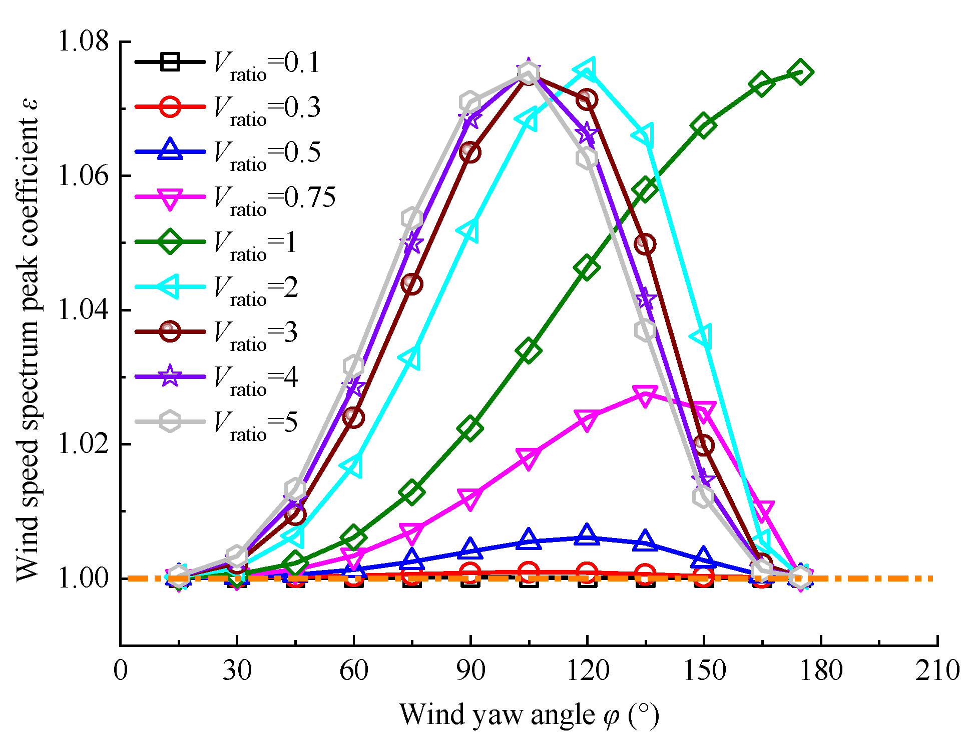
Figure 8 shows the change regulation of the wind speed spectrum peak at different wind yaw angles and different Vratio values, in which the amplification coefficient ε represents the ratio of the peak between the moving point and the static point. Generally, the wind speed spectrum peak changes with the wind yaw angles into the sinusoidal curve.
When the Vratio value is 0.1 or 0.3, the wind speed spectrum peak of the moving point roughly coincides with the peak of the static point at different wind yaw angles. That is, when the vehicle’s moving speed is small, the influence of movement can be neglected.
When the Vratio is 0.5 and φ is 120°, the wind speed spectrum peak is at its maximum and reaches its minimum at 15° and 175°. The influence of the vehicle’s moving speed should be considered, and the maximum increase rate of the wind speed spectrum peak could be 0.6%.
When the Vratio is 0.75 and φ is 135°, the wind speed spectrum peak is at its maximum and reaches its minimum at 15° and 175°. The maximum increase rate of the wind speed spectrum peak could be 2.7%.
When the Vratio is 1 and φ is 175°, the wind speed spectrum peak is at its maximum. The maximum increase rate of the wind speed spectrum peak is 7.6%. While this would not happen in the condition where φ is 175°. That is, when the wind is coming from behind the vehicle. There is no sense for this condition. The wind speed spectrum peak is at its minimum at 15°.
When the Vratio is 2, the wind speed spectrum peak is at its minimum at a wind yaw angle of 15° and is at its maximum at 120°. The maximum increase rate of the wind speed spectrum peak could be 7.6%. When the Vratio increases to 5 from 3, the wind speed spectrum peak is also at its minimum at 15° and reaches its maximum at 105°. The maximum increase rate of the wind speed spectrum peak could be 7.5%. That is, when the Vratio value is small, the influence of the vehicle’s moving speed is low, and the wind speed spectrum is close to that of the static point.
In a natural wind environment, the influence of the vehicle’s movement must be considered, and the wind speed spectrum peak increased by only about 8.0% at a wind yaw angle of 105°. That is, the wind speed spectrum peaks are roughly the same at different wind yaw angles and Vratio values. When the Vratio is larger than 1, the maximum wind speed spectrum peaks are all increased by 8.0%.
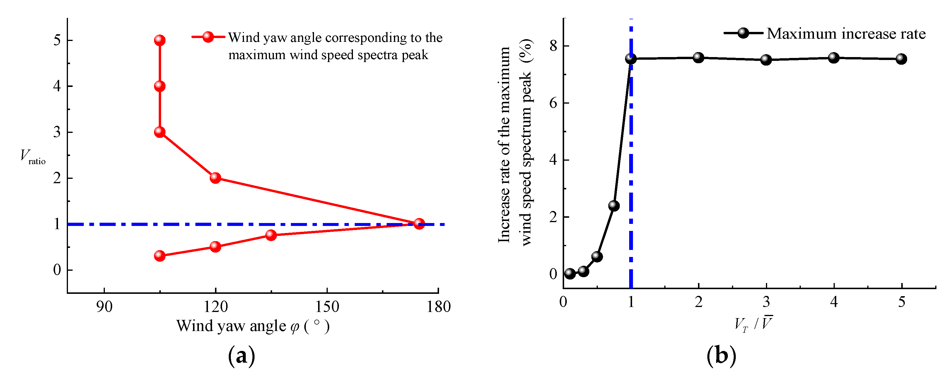
The wind speed spectrum peak of a moving point is larger than that of a static point. The change law is shown in Figure 9a. As the Vratio value increases, the wind yaw angle corresponding to the maximum wind speed spectrum peak was firstly increased and then decreased. When the Vratio value is smaller than 1, the frequencies corresponding to the wind speed spectrum peak are increased with the increasing Vratio values. When the Vratio value is larger than 1, the frequencies corresponding to the wind speed spectrum peak were decreased and then remained unchanged for Vratio values larger than 3. As the Vratio value increased, the wind yaw angle corresponding to the maximum value of ε was firstly increased and then decreased.
In Figure 9b, the maximum wind speed spectrum peak increase rate is shown. Under the condition that the Vratio value is larger than 1, the wind speed spectrum peaks increase by 8% and exhibit little change. The wind speed spectrum of a moving point could be considered to have just moved to the right, with small changes in the values. Under the condition that the Vratio value is smaller than 1, the maximum wind speed spectrum peak is increased with the increasing Vratio.
It is obviously known that, for different Vratio values, the worst working condition is not at a wind yaw angle of 90°. In a natural wind environment, the ratio of the train vehicle’s moving speed to the wind speed could reach 5 or larger. The most adverse working conditions are found under a wind yaw angle of 105°.
4.3. Discussion of Frequencies Corresponding to Wind Speed Spectrum Peak
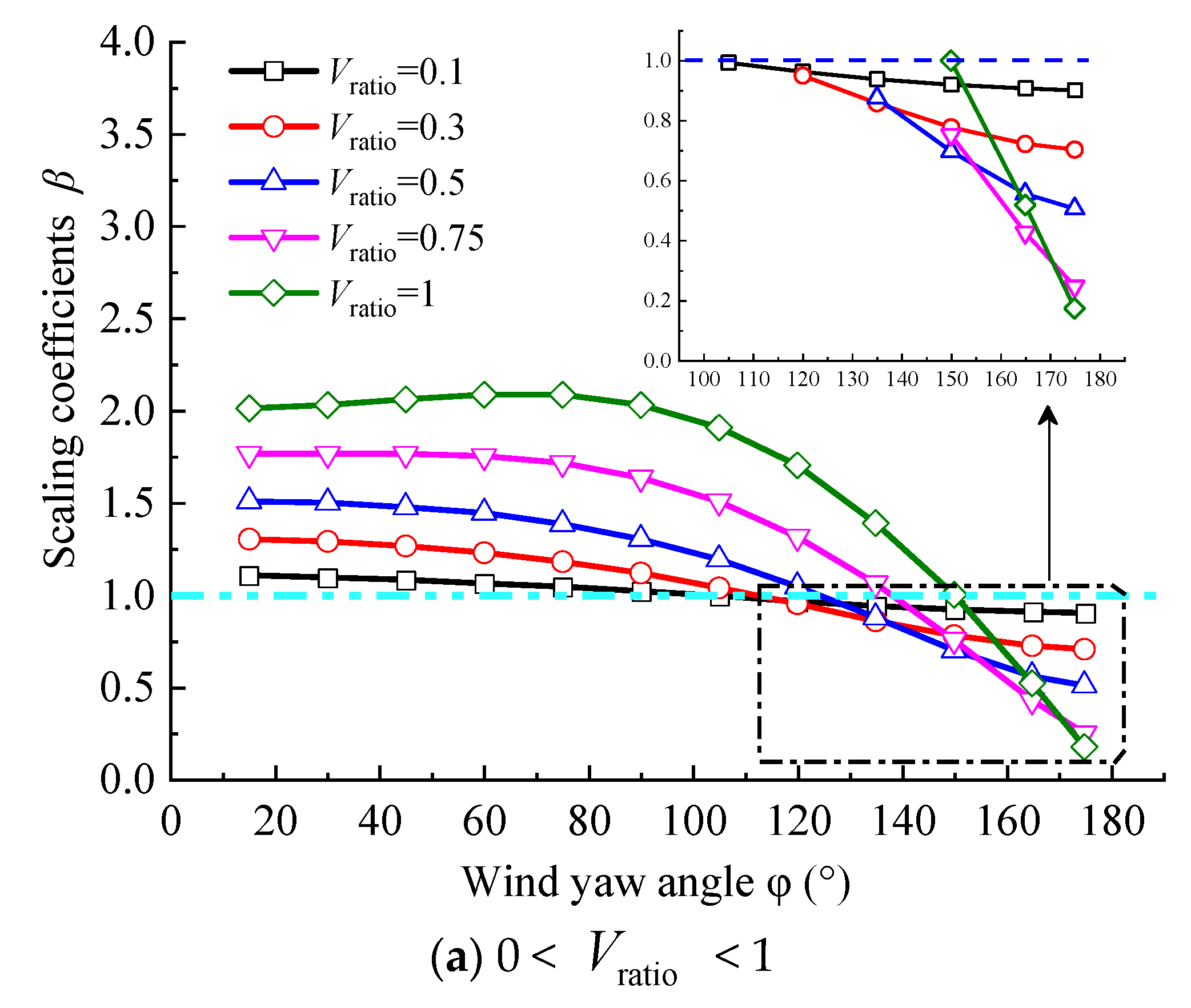
In Figure 10, the scaling coefficients of frequencies corresponding to the wind speed spectrum peak are shown. Generally, the scaling coefficients are increased. That is, for a moving point, the frequencies corresponding to the wind speed spectrum peak are larger than those of a static point. Scale coefficients β represent the frequency corresponding to the maximum value of the wind speed spectrum of a moving vehicle to the static.
From Figure 10a, when the Vratio is 0.1 and the wind yaw angle is 105°, 120°, 135°, 160° or 175°, the frequencies corresponding to the wind speed spectrum peak of a moving point are smaller than those of a static point. The frequencies show little change as the wind yaw angles increase. When the Vratio is 0.5 and the wind yaw angle is 135°, 150°, 165° or 175°, the same rule is true. The frequency increases as the wind yaw angle increases. When the Vratio value is 1 and the wind yaw angle is 150°, 165° or 175°, the frequency corresponding to the wind speed spectrum peak of a moving point is smaller than that of a static point. That is, the scaling coefficient is smaller than 1. When the wind yaw angle is 45°, the frequency corresponding to the wind speed spectrum peak of a moving point is the same as that of a static point. In addition, the frequency increases as the wind yaw angle increases. When the wind yaw angle is small, the wind speed spectrum peak of the moving point is mainly caused by the longitudinal wind speed spectrum, and the influence of the transverse wind speed spectrum is small. As the wind yaw angle gradually increases, the influence of the transverse wind speed spectrum also gradually increases.
From Figure 10b, when the Vratio is 2, 3, 4 or 5, the frequencies corresponding to the wind speed spectrum peak first are firstly increased and then decreased. When the wind yaw angle is 90°, the frequency corresponding to the wind spectrum peak of a moving vehicle is at its maximum. The maximum scaling coefficient β can reach 10 and the minimum coefficient β can reach 6 when the Vratio value is 5. When the Vratio value is 0.1 or 0.5, the maximum scaling coefficient β is smaller than 2 at different wind yaw angles. That is, when the wind direction is perpendicular to the vehicle’s moving direction, the frequencies corresponding to the wind speed spectrum peak of a moving vehicle are at their largest.
5. Coherence Function
The cross-correlation function of the wind speed at points P and P´ in Figure 3 can be written as follows:
where and are, respectively, the longitudinal wind speeds at points P and P’ at time t and .
The time delay can be transformed into an equivalent spatial interval according to Taylor’s freezing hypothesis in Figure 2. Equation (24) can be presented as the correlation characteristics of points P and :
where is the cross-power spectral density of two points on a moving vehicle with a distance . is the power spectral density of a single point.
By substituting Equation (27) into Equation (28), Equation (27) can be written as follows:
could be presented as follows:
In Equation (31), Cu is the correlation coefficient which could not evaluate the influence of the turbulence integral scale on the correlation characteristics.
Jakobsen [24] proposed an empirical model with appropriate corrections as follows:
where c1, c2 and c3 are the parameters to be fitted. The parameters are dimensioned, and Equation (32) can be corrected as follows:
The correlation coefficients can then be obtained from Equation (33). However, the most important problem is that the expression for a correlation function cannot be obtained easily. Wu [18] obtained the change law of the correlation function using an integral approach. Considering the wind speed spectrum peak, when the Vratio value is larger than 1, the increasing rate could reach 8%. After comprehensive consideration, when the vehicle’s moving speed is larger than the wind speed, the wind speed spectrum and correlation characteristics should be considered.
In Figure 11, some of the coherence function points on the vehicle at different moving speeds are shown. It could be known that the coherence function increases with the increasing speed ratio of the vehicle’s moving speed to the wind speed. The correlation characteristics of the moving vehicles, which are of great influence, could be investigated by wind tunnel tests.
6. Conclusions
An investigation of the wind speed spectrum characteristics of a moving vehicle under turbulent crosswinds has been conducted. The influencing factors, including the ratio of the vehicle speed to the wind speed, and the wind yaw angle from 15° to 175°, were analyzed. Some conclusions were obtained:
- The wind speed spectrum peak changes with the wind yaw angles into the sinusoidal curve at different Vratio values. When the Vratio value is 0.1, the wind speed spectrum peak of the moving point gradually coincides with the peak of the static point at different wind yaw angles. As the Vratio is increased, the wind speed spectrum peak is at its maximum under smaller wind yaw angles, which is from 175° to 105° generally.
- As the wind yaw angle gradually increases, the influence of the transverse wind speed spectrum also gradually increases. When the Vratio is 2, 3, 4 or 5, the frequency corresponding to the wind speed spectrum peak is first increased and then decreased.
- The increases in both coherence and the power spectrum contribute to the larger aerodynamic forces and wind-induced vehicle vibration as the speed ratio increases. The correlation characteristics of the moving vehicles, which are of great influence, could be investigated by wind tunnel tests in further studies.
- The wind speed spectrum and cross-correlation characteristics of moving points could be experimentally investigated in wind tunnels to further analyze the mathematical model. Furthermore, investigation of the aerodynamic characteristics of the moving vehicles should also be conducted.
Funding
The author disclosed receipt of the following financial support for the research, authorship, and/or publication of this article: the research described in this article was financially supported by the Natural Science Foundation of China (grant no.: 52078438); the Natural Science Foundation of the Southwest University of Science and Technology (grant no: 21ZX7148); the key research base of the Humanities and Social Sciences of Sichuan Education Department of Chengdu Information Engineering University—Key project of the Meteorological Disaster Forecast, Early Warning and Emergency Management Research Center in 2022 (grant no.: ZHYJ22-ZD02); and the Wind Engineering Key Laboratory of Sichuan Province (grant no.: WEKLSC202302).
Institutional Review Board Statement
Not applicable.
Informed Consent Statement
Not applicable.
Data Availability Statement
Data are contained within the article.
Conflicts of Interest
The author declares no conflict of interest. The funders had no role in the design of the study; in the collection, analyses, or interpretation of data; in the writing of the manuscript; or in the decision to publish the results.
References
- Guo, W.W.; Xia, H. Dynamic responses of long-span bridges and running safety of trains under wind action. China Railw. Sci. 2006, 2, 137–139. [Google Scholar] [CrossRef]
- Ma, C.M.; Duan, Q.S.; LI, Q.S.; Chen, K.J.; Liao, H.L. Buffeting forces on static trains on a truss girder in turbulent crosswinds. J. Bridge Eng. 2018, 23, 04018086. [Google Scholar] [CrossRef]
- Huang, T.M.; Feng, M.C.; Huang, J.; Ma, J.M.; Yi, D.; Ren, X. Aerodynamic stability of high-speed vehicle passing bridge tower in different lanes under crosswind conditions. J. Wind Eng. Ind. Aerodyn. 2023, 242, 105560. [Google Scholar] [CrossRef]
- Li, M.; Li, M.S.; Yang, Y. Strategy for the determination of unsteady aerodynamic forces on elongated bodies in grid-generated turbulent flow. Exp. Therm. Fluid Sci. 2020, 110, 109939. [Google Scholar] [CrossRef]
- Li, X.Z.; Qiu, X.W.; Zhang, J.; Wang, M. Aerodynamic characteristics of fully enclosed sound barrier induced by the passing trains with 400 km/h. J. Wind Eng. Ind. Aerodyn. 2023, 241, 105518. [Google Scholar] [CrossRef]
- Li, Y.L.; Qiang, S.Z.; Liao, H.L.; Xu, Y.L. Dynamic of wind-rail vehicle-bridge system. J. Wind Eng. Ind. Aerodyn. 2005, 93, 483–507. [Google Scholar] [CrossRef]
- Li, X.Z.; Xiao, J.; Liu, D.J.; Wang, M. Fluctuating wind velocity spectra of moving vehicle under horizontal crosswind. Sci. Sin. Tech. 2016, 46, 1263–1270. [Google Scholar] [CrossRef]
- Li, X.Z.; Xiao, J.; Liu, D.J.; Wang, M. An Analytical Model for the Fluctuating Wind Velocity Spectra of a Moving Vehicle. J. Wind Eng. Ind. Aerodyn. 2017, 164, 34–43. [Google Scholar] [CrossRef]
- Xu, Y.L.; Zhang, N.; Xia, H. Vibration of coupled train and cable-stayed bridge system in crosswinds. Eng. Struct. 2006, 26, 1389–1406. [Google Scholar] [CrossRef]
- Cai, C.S.; Chen, S.R. Framework of vehicle-bridge wind dynamic analysis. J. Wind. Eng. Ind. Aerodyn. 2004, 92, 579–607. [Google Scholar] [CrossRef]
- Cooper, R.K. Atmospheric Turbulence with Respect to Moving Ground Vehicles. J. Wind Eng. Ind. Aerodyn. 1984, 17, 215–238. [Google Scholar] [CrossRef]
- Watkins, S.; Saunders, J.W.; Hoffemann, P.H. Turbulence Experienced by Moving Vehicles. Part I. Introduction and Turbulence Intensity. J. Wind Eng. Ind. Aerodyn. 1995, 57, 1–17. [Google Scholar] [CrossRef]
- Watkins, S.; Milbank, J.; Loxton, B.J.; Melbourne, W.H. Atmospheric Winds and Their Implications for Micro air Vehicles. Aiaa J. 2006, 44, 2591–2600. [Google Scholar] [CrossRef]
- Hu, P.; Lin, W.; Yang, D.G.; Han, Y.; Yan, C. Fluctuating wind speed spectrum of a moving vehicle under crosswinds. China J. Highw. Transp. 2018, 31, 101–109. [Google Scholar]
- Hu, P.; Han, Y.; Cai, C.S.; Cheng, W.; Lin, W. New analytical models for power spectral density and coherence function of wind turbulence relative to a moving vehicle under crosswinds. J. Wind Eng. Ind. Aerodyn. 2019, 188, 384–396. [Google Scholar] [CrossRef]
- Yu, M.; Liu, J.; Liu, D.; Chen, H.; Zhang, J. Investigation of aerodynamic effects on the high-speed train exposed to longitudinal and lateral wind velocities. J. Fluids Struct. 2016, 61, 347–361. [Google Scholar] [CrossRef]
- Wu, M.X.; Li, Y.L.; Chen, X.Z.; Hu, P. Wind spectrum and correlation characteristics relative to vehicles moving through cross wind field. J. Wind Eng. Ind. Aerodyn. 2014, 133, 92–100. [Google Scholar] [CrossRef]
- Su, Y.; Li, M.S.; Yang, Y.; Mann, J.; Liao, H.; Li, X. Experimental investigation of turbulent fluctuation characteristics observed at a moving point under crossflows. J. Wind Eng. Ind. Aerodyn. 2020, 197, 104079. [Google Scholar] [CrossRef]
- Balzer, L.A. Atmospheric turbulence encountered by high-speed ground transport vehicles. J. Mech. Eng. Sci. 1977, 19, 227–235. [Google Scholar] [CrossRef]
- Kármán, T.V. Progress in the statistical theory of turbulence. Physics 1948, 34, 530–539. [Google Scholar] [CrossRef]
- Bullen, H.I. Gusts at low altitude in North Africa. R. Aircr. Establ. Tech. Note Struct. 1961, 304, 1–10. [Google Scholar]
- Cheng, W.C. On the value of the von Kármán constant in the atmospheric surface layers over urban surfaces. J. Wind Eng. Ind. Aerodyn. 2023, 241, 105547. [Google Scholar] [CrossRef]
- Sharma, M.K.; Verma, M.K.; Chakraborty, S. On the energy spectrum of rapidly rotating forced turbulence. Phys. Fluids. 2018, 30, 115102. [Google Scholar] [CrossRef]
- Jakobsen, J.B. Span-wise structure of lift and overturning moment on a motionless bridge girder. J. Wind. Eng. Ind. Aerodyn. 1997, 69–71, 795–805. [Google Scholar] [CrossRef]
Figure 1.
Correlation functions.

Figure 2.
Two points and their equivalent points on a moving vehicle.

Figure 3.
Validation of wind speed spectrum of a moving vehicle based on von Kármán spectrum [11].
Figure 3.
Validation of wind speed spectrum of a moving vehicle based on von Kármán spectrum [11].

Figure 4.
Experimental setups for the wind fields (unit: cm): (a) schematic diagrams of the experimental setups; and (b) Turbulent Flow Instrument.
Figure 4.
Experimental setups for the wind fields (unit: cm): (a) schematic diagrams of the experimental setups; and (b) Turbulent Flow Instrument.

Figure 5.
Comparison of the turbulence flow PSD and von Kármán PSD.

Figure 6.
Wind speed spectra of a moving vehicle.

Figure 7.
Wind speed spectra of a moving vehicle at different wind yaw angles.

Figure 8.
Wind speed spectrum peak coefficients.

Figure 9.
Change law of wind speed spectrum peak coefficients: (a) wind yaw angles corresponding to maximum wind speed spectrum peak; (b) increase rate of the maximum wind speed spectrum peak.
Figure 9.
Change law of wind speed spectrum peak coefficients: (a) wind yaw angles corresponding to maximum wind speed spectrum peak; (b) increase rate of the maximum wind speed spectrum peak.

Figure 10.
The frequency corresponding to the wind speed spectrum peak.


Figure 11.
Coherence function of points on vehicle at different Vratio values.


Table 1.
Characteristics of the typical types of turbulent flows.
| Mean Wind Speed (m/s) | Turbulence Integral Scale | Turbulence Intensity | ||||
|---|---|---|---|---|---|---|
| Lu (m) | Lv (m) | Lw (m) | Iu (%) | Iv (%) | Iw (%) | |
| 7.770 | 0.685 | 0.245 | 0.217 | 8.634 | 7.757 | 6.944 |
Note: represents the longitudinal direction; represents the lateral direction; and represents the vertical direction.
Disclaimer/Publisher’s Note: The statements, opinions and data contained in all publications are solely those of the individual author(s) and contributor(s) and not of MDPI and/or the editor(s). MDPI and/or the editor(s) disclaim responsibility for any injury to people or property resulting from any ideas, methods, instructions or products referred to in the content. |
© 2023 by the author. Licensee MDPI, Basel, Switzerland. This article is an open access article distributed under the terms and conditions of the Creative Commons Attribution (CC BY) license (https://creativecommons.org/licenses/by/4.0/).
Share and Cite
MDPI and ACS Style
Duan, Q. Wind Speed Spectrum of a Moving Vehicle under Turbulent Crosswinds. Appl. Sci. 2023, 13, 12054. https://0-doi-org.brum.beds.ac.uk/10.3390/app132112054
AMA Style
Duan Q. Wind Speed Spectrum of a Moving Vehicle under Turbulent Crosswinds. Applied Sciences. 2023; 13(21):12054. https://0-doi-org.brum.beds.ac.uk/10.3390/app132112054
Chicago/Turabian StyleDuan, Qingsong. 2023. "Wind Speed Spectrum of a Moving Vehicle under Turbulent Crosswinds" Applied Sciences 13, no. 21: 12054. https://0-doi-org.brum.beds.ac.uk/10.3390/app132112054
Note that from the first issue of 2016, this journal uses article numbers instead of page numbers. See further details here.