1. Introduction
The demand for bandwidth is rapidly increasing, primarily fueled by the proliferation of interconnected devices on the internet. This increase, combined with the high inertia in updating the physical layer, has accentuated the bottleneck in customer access to the network. In response, due to their high cost-effectiveness, many are increasingly considering passive optical networks (PONs) as a promising solution because of their ability to achieve speeds exceeding 100 Gbit/s and the need to ensure the quality of service (QoS) standards that are established in different territories [
1,
2]. Passive optical networks (PON) have technologically evolved with the use of optical technologies such as advanced modulation formats, coherent optical networks, and integrated photonics. The latter technology allows for the design and production of these advanced devices on chips, which enhances their portability and reproducibility [
2,
3]. This evolution has also seen the establishment of standards such as asynchronous PON (APON), broadband PON (BPON), Ethernet PON (EPON), and 10-gigabit PON (XG-PON), thus enabling the introduction of optical communication at speeds near 10 Gbit/s and the exchange of essential protocols such as Ethernet [
4,
5].
The creation of full-service access network (FSAN) PONs was intended to meet the growing bandwidth demand. These PONs have transmission speeds of up to 40 Gbit/s and utilize multi-level communication protocols such as quadrature amplitude modulation (QAM), quadrature phase shift keying (QPSK), and phase shift keying (PSK) to enhance the spectral efficiency. Wavelength division multiplexing (WDM) is also utilized to transmit information through multiple channels, resulting in rigid frequency grids within a spectrum section [
3]. Implementing approaches that employ multiple lasers to replicate each frequency of the International Telecommunication Union (ITU) grid has significantly increased network speed and efficiency. However, deploying this technology has proven costly, primarily due to the requirement for multiple lasers and the considerable economic investment that it requires. Additionally, achieving high phase coherence between each laser frequency has posed a significant challenge, thereby restricting the capacity and effectiveness of these approaches [
6].
Other researchers have taken a different approach to optimizing the utilization of existing infrastructure without introducing new PON standards [
2,
7], thereby avoiding network cost escalation. Developers have created dynamic bandwidth allocation (DBA) algorithms to achieve this. Designers have created these algorithms to share network resources by taking advantage of carrier availability when customers do not require an exclusive channel and by making requests at specific times [
8,
9]. Additionally, some strategies aim to distribute network requests effectively by utilizing heuristics that optimize latency; while these approaches achieve faster response speeds, their networks are rigid and do not permit the utilization of various modulation formats and wavelengths. Alternative methods of achieving dynamic bandwidth allocation involve the utilization of multiple channels enabled by wavelength division multiplexing (WDM) infrastructure and the development of algorithms such as Dynamic Wavelength and Bandwidth Allocation (DWBA) or Routing and Spectrum Assignment (RSA), which leverage the capabilities of WDM technology. Despite their potential to enhance the network efficiency, the significant separation between wavelengths (200 GHz, 100 GHz, and 50 GHz) limits optimal spectrum utilization, particularly for requests that require a low transfer rate—as is the case for Internet of Things (IoT) devices. Additionally, these approaches do not account for the use of different multi-level modulation formats, which could help to reduce the portion of the spectrum needed [
10,
11].
A few methodologies have been proposed in the literature that employ machine learning and optimization techniques to enhance the spectral efficiency of the WDM approach [
12,
13,
14]. This optimization aims to transmit the maximum amount of data in the shortest possible time and achieve spectrum allocation. These approaches have achieved promising results, such as minimizing the required spectrum, predicting future demands, and efficient network management. However, they carry a significant computational cost that impedes their use in real-life scenarios, where processing time and hardware device implementation must be ensured [
15,
16]. Alternatives employing flexible networking approaches are available, integrating radio frequency infrastructures, wireless systems, and optical networks. This approach is called the Multi-Stratum Resources Optimization with Converged Radio over Fiber and 5G Network (C-RoFN) architecture, and they enable the comprehensive maximization of resources, including radio frequency, optical spectrum, and BBU processing capacity. The primary goal is to enhance the radio coverage and meet quality of service standards; while these methodologies focus on spectrum allocation, they revolve around integrating diverse transmission sources, contrary to spectral allocation within an optical network. Consequently, these approaches cannot be adapted as a solution to the problem at hand because their algorithms are not tailored to the specific requirements of a PON network as they are designed for multiple sources. Moreover, these approaches encompass different physical infrastructures that the same service provider does not invariably control. Thus, their application may be accompanied by elevated implementation costs when implemented in real-world scenarios [
17].
Another strategy to optimize the optical spectrum involves the utilization of spatial division multiplexing (SDM) within multi-core fibers. This approach aims to enhance the spectral efficiency by capitalizing on the multiple channels inherent to this fiber type. Furthermore, this methodology employs a self-organizing feature mapping (SOFM) neural network to discern potential crosstalk interference among the channels, thereby mitigating the blocking probability. This conceptual framework facilitates the allocation of dedicated channels for data transmission. Despite its commendable benefits in augmenting data capacity, this inventive approach encounters constraints rooted in its reliance on multi-core fibers. These fibers are constrained by limitations concerning transmission distances. Additionally, they introduce intricacies in configuring PON networks due to their inadequate compatibility and the requisite devices for implementation. Consequently, this circumstance creates substantial costs in system deployment. Furthermore, the efficacy of this approach is contingent upon the availability of optical sources, constituting a significant limitation in furnishing each fiber core [
18].
To address the challenges posed by spectrum allocation and the need to create a lower-cost approach, researchers have proposed heuristic methods that utilize multiple modulation formats and reduce the WDM grid spacing to 12.5 and 6.25 GHz values. These approaches, collectively called Routing, Modulation Level, and Spectrum Assignment (RMLSA), are crucial in establishing a flexible optical network to maximize spectral efficiency [
19,
20,
21]. RMLSA approaches employ multi-level modulation formats such as QAM, PSK, and QPSK to adjust the modulation level and type to accommodate requests adaptively, thus reducing the required spectrum and complying with the distance constraints of different network requests [
13,
22,
23]. Recent research has adopted genetic algorithms to find an optimal solution to the RMLSA problem. This approach simultaneously considers the routing and permutation of requests to explore a more significant portion of the RMLSA solution set than current metaheuristics. Although these approaches offer highly efficient solutions, their computational cost is high, challenging their feasibility in a real operating environment [
24]. The RMLSA strategy enables an increase in simultaneous requests, but the economic costs of adding wavelengths constrain its potential.
A practical solution to increase the number of wavelengths without significantly escalating costs is the utilization of optical frequency combs (OFCs). An OFC is an optical source with a spectrum composed of a series of discrete frequency lines that are equally spaced and highly coherent [
25,
26,
27]. The described properties indicate its potential as a solution for the generation of OFCs. As of 2023, WDM communication systems with speeds approaching 1.84 Pbit/s have been achieved using up to 37 wavelengths [
28,
29,
30]. Different techniques for the generation of OFCs have been proposed, such as electro-optic modulation, acousto-optic modulation, ring recirculating modulation, Mach–Zehnder modulators with microresonators, and four-wave mixing. While many of these techniques can achieve comb generation, they carry high economic costs and present considerable insertion losses [
31,
32,
33,
34].
The use of micro-resonators (MRR) in integrated photonics has shown great potential in generating optical frequency combs (OFCs) with multiple wavelengths. Recent studies have demonstrated the successful generation of up to 179 comb lines [
35]. This approach involves coupling a laser to an optical microresonator, adjusting the power (
), and detuning the (
) parameters at a resonant frequency to generate multiple wavelengths [
36]. This approach offers device stability, reproducibility, and scalability. In [
37,
38], the authors propose this approach as an alternative to parallel lasers in WDM systems. This study addresses crucial aspects such as the optical linewidth, power per channel in the comb, and the optical carrier’s signal-to-noise ratio. Furthermore, the scalability of a comb source for ultra-high-capacity systems is investigated, as well as the optimization of the above-mentioned parameters. These studies show significant potential in the application of this technology in PONs. However, researchers widely use optical microresonators to transmit information in long-distance networks, where the transmission paths typically have the same distance. The non-uniform distribution of comb wavelengths following a sech2 function poses a problem, as additional optical processing is required to ensure the adequate transmission of OSNR. Existing spectrum allocation methods rely on the uniform spectral power of each wavelength, requiring optical processing before use, which increases the economic costs of implementation. A PON, on the other hand, has a point-to-multipoint structure with variable distances, which allows for the direct utilization of the comb generated by the MRR.
The initial concept offers significant advantages, including cost reductions and the potential to incorporate more optical comb wavelengths, thereby increasing the potential of RMLSA methods with WDM. These advantages are critical for last-mile networks, which must meet the demands for flexible network speeds of 50 Gbit/s, 100 Gbit/s, and 400 Gbit/s while accommodating 5G mobile transport, IoT device traffic, spectrum optimization, increased transmission speeds, and other challenges without significantly raising investment costs [
2,
3,
7]. However, there is currently no evidence of a spectrum allocation strategy for PON networks using the optical comb of an MRR. This study proposes a methodology for the generation, transmission, and allocation of spectra using an RMLSA-WDM approach with MRR to address the issue. Hence, the work provides the following main contributions.
A method for the deterministic generation of OFCs with a standardized ITU-grid FSR. The values are 12.5 GHz, 50 GHz, 100 GHz, and 200 GHz.
The design of a photonic system with machine learning to select the OFC with the most suitable characteristics for customers with different bandwidth requests and transmission distances.
A methodology for spectrum allocation with multi-level modulation and WDM focus that considers the non-uniformity of the OFC.
2. Materials and Methods
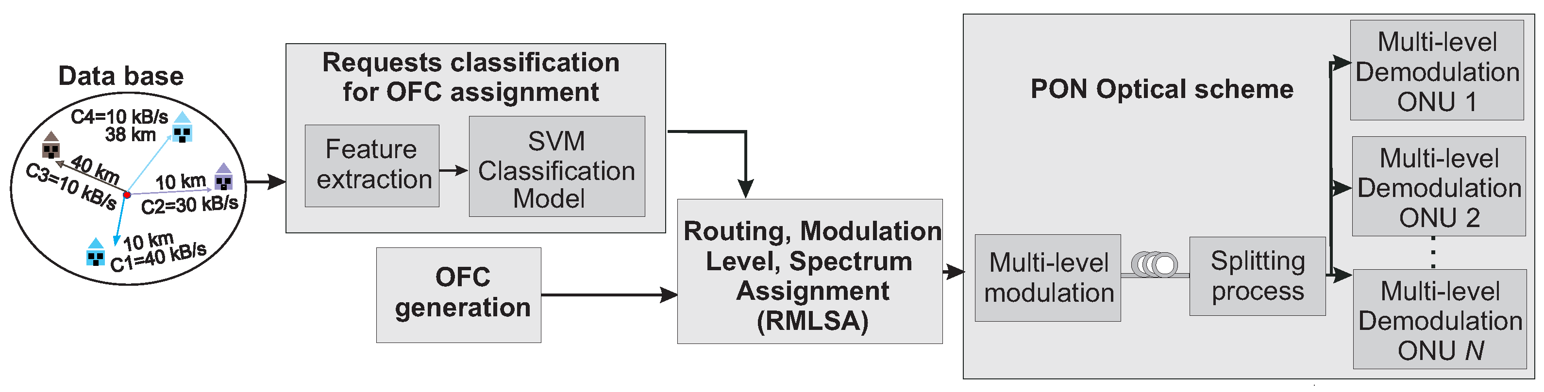
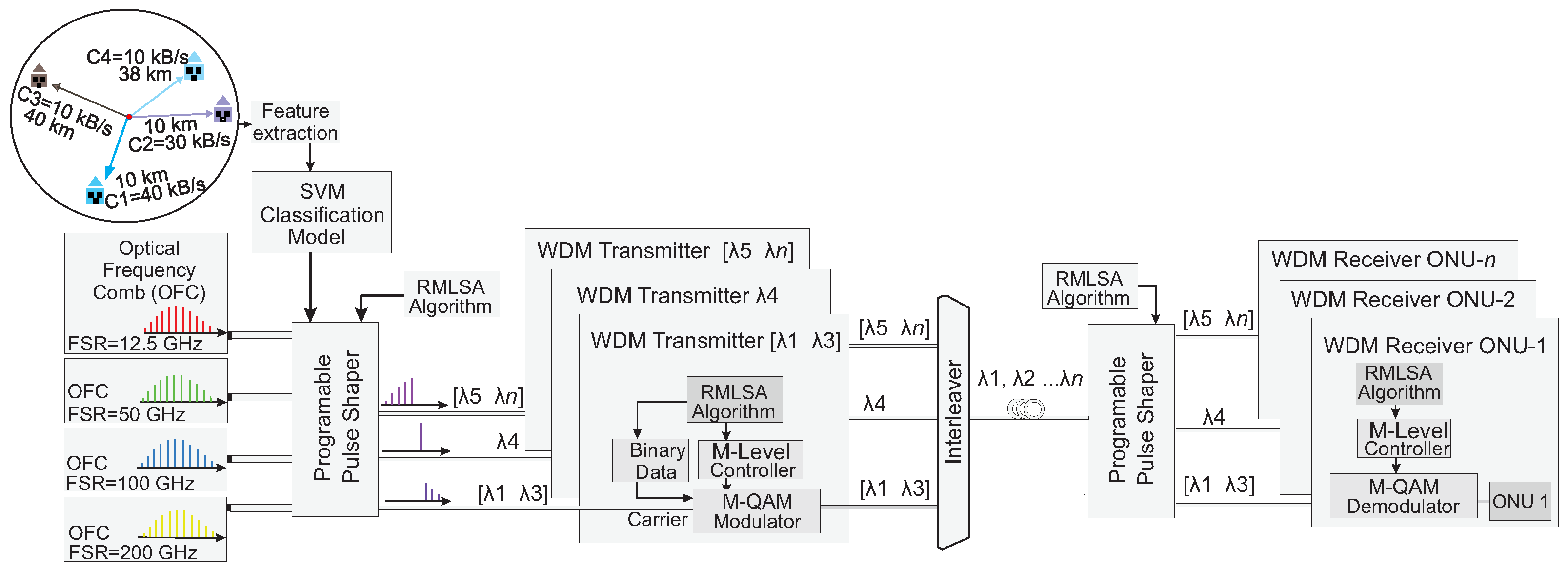
The methodology proposes a three-stage methodology for the selection of the appropriate type of OFC to transmit information in a PON network. The first stage involves developing a machine learning algorithm to select the appropriate OFC based on the network’s characteristics. In the second stage, a reliable path and a deterministic generation strategy for the OFC are defined. Finally, an RMLSA algorithm is implemented to efficiently allocate the generated spectrum using a programmable line-by-line pulse shaper. This work validates the algorithm in various request scenarios and compares its performance to that of other approaches in the literature.
Figure 1 shows the proposed methodology’s diagram.
2.1. Database
Developing an annotated database of customer requests is essential to validate the performance of the proposed machine learning algorithm. The design of this database must consider the distance between customers and the central network office, the required communication speeds, and the number of customers making requests. To model these features, discrete uniform random variables are used to model request characteristics. We justify this modeling approach to validate network performance under different request scenarios and ensure that each situation has an equal probability of occurrence, and it reflects high, low, and average bandwidth consumption cases. The database ranges are determined based on typical operational scenarios of a PON network and future bandwidth requirements [
39]. The database includes the characteristics outlined in
Table 1.
Table 1 illustrates request scenarios involving 200 requests, varying distances of 80 km, and speeds of up to 250 Gbit/s. The database contains a set of 1400 requests, which present non-heterogeneous scenarios with bandwidths of different magnitudes. These considerations aid in the validation process by considering interesting scenarios such as IoT devices, last-mile users, and users with substantial bandwidth needs that may necessitate super-channel implementation. In this database, we consider four distinct classes labeled as follows: class 1 corresponds to a frequency of 12.5 GHz, class 2 to 50 GHz, class 3 to 100 GHz, and class 4 to 200 GHz. Each label represents the OFC generation system’s free spectral range (FSR). We base the process of assigning labels to the database on the following criteria.
Firstly, we ensure that the number of available lines per comb exceeds the number of customers requesting the service. If the number of requests exceeds the available lines, we assign the comb with bandwidth capacity and avoid using super-channels.
Secondly, we ensure that the total bandwidth requested by the customers does not exceed the available bandwidth of the optical comb.
2.2. Request Classification for OFC Assignment
This study uses an SVM to identify the appropriate FSR in a network request scenario. The classification process involves two phases: feature extraction and the computation of optimal model parameters. The goal is to construct a model that enables separability and correctly identifies the four classes. We do not consider deep learning techniques due to their unsuitability for tabular data. Deep learning models excel in handling unstructured data such as text and images but struggle to leverage the fixed feature set of tabular data effectively [
40]. Furthermore, their higher computational cost conflicts with the real-time processing demands of this research. Instead, we confidently choose an SVM, as they efficiently handle tabular data and achieve problem separability while meeting our computational requirements. However, we conduct comparison tests with a convolutional neural network (CNN-1D) to verify its performance.
2.2.1. Feature Extraction
We compute the key features that describe the trends and variability of the request set in order to achieve a representation space that is highly separable (see
Table 2). This approach aims to construct a feature space that captures the essential information of the request, enabling the identification of the FSR that best matches the characteristics of the request.
Here, is the mean value of the data and is the speed in Gbit/s of each request.
2.2.2. Training and Classification Settings for Machine Learning Methods
In this study, we employ a multiclass support vector machine with the one vs. all strategy to perform the classification process. Implementing a Gaussian kernel with an adaptive radius enhances the separability of the representation space. We utilize the Sequential Minimal Optimization (SMO) algorithm to determine the optimal parameters of the model. To ensure proper training, we implement a Monte Carlo algorithm that employs a cross-validation strategy, and divide the data into 70% for training and 30% for testing. The method randomly distributes the data in each iteration, and we perform 200 repetitions of each one. The performance metric for this experiment is computed as the confusion matrix. We select this classification method for its high accuracy of over 95% and its reasonable computational cost for the application. The Results section provides a comparison of this work with other methods in the literature, such as K-nearest neighbors (KNN), artificial neural networks (ANN), and convolutional neural network 1D (CNN-1D).
For the KNN approach, we select a value of K equal to 4 and employ the Euclidean distance metric to assess the similarity between the training set and the new instances for classification. Furthermore, we assign equal weights to all neighbors when determining the class. On the other hand, the ANN utilizes the backpropagation algorithm with two hidden layers, each consisting of 15 neurons, all employing the hyperbolic tangent activation function (tansig). At the end of the structure, the output layer is responsible for classifying the four types of optical combs.
The CNN-1D architecture consists of three blocks, each containing 1D convolutional layers. Each block has seven filters with kernel sizes of 64, 128, and 192. The activation function employed is ReLU, and each block is supplemented with layer normalization. Subsequently, the CNN incorporates a global average pooling 1D layer, which reduces the output dimensions to a singular vector. This vector is then integrated with a fully connected layer utilizing a Softmax activation function. Lastly, a classification layer is applied. The training process involves the utilization of the Adam optimizer across 15 epochs, which are managed through mini-batches of size 27 and supported by validation data.
2.3. OFC Generation
The proposed solution to obtain the maximum number of wavelengths is an OFC generation system based on the method in [
41], which uses multiple thermally controlled optical microring resonators to shift the frequency of each comb line. Subsequently, these lines are combined using an interleaver to form a single optical comb with a smaller line spacing known as the FSR. Although this methodology requires multiple microring resonators (MRRs), it offers the advantage of having several wavelengths for spectrum assignment, which is crucial in solving this problem. This approach creates flexible WDM grids with different line spacings (12.5 GHz, 50 GHz, 100 GHz, and 200 GHz). We choose silicon nitride MRRs (Si
N
) because of their ease of fabrication, reproducibility, low optical losses, compatibility with standard CMOS technology, and ability to deterministically generate optical combs [
41,
42].
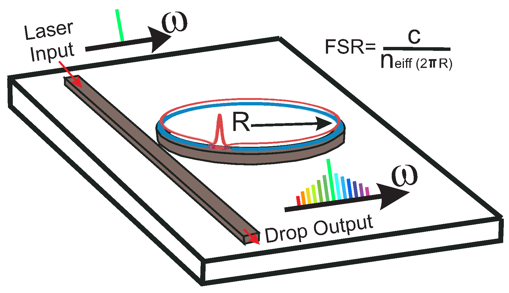
An MRR is a compact, integrated optical device typically fabricated on a silicon substrate. It consists of a ring-like or disk-like waveguide structure that allows light to circulate within it. This circular or looped design enables optical resonance, where specific optical frequencies or wavelengths, become trapped and accumulate within the microresonator (see
Figure 2). As light is input into the microresonator through an optical waveguide, it circulates within the closed-loop structure, and, due to the constructive interference of the trapped wavelengths, it intensifies over multiple round trips. This phenomenon generates an optical frequency comb.
Designing an MRR to generate frequency combs with a desired free spectral range (FSR) involves careful adjustment of the resonator’s radius, as the FSR is inversely proportional to the resonator’s radius. A larger radius results in a smaller FSR, while a smaller radius leads to a larger FSR. Managing optical losses through material selection and fabrication techniques is crucial to achieving efficient comb generation and maintaining a high Q-factor. Optimizing the coupling factor by tailoring the waveguide designs ensures effective light interaction with the microresonator, collectively allowing precise control over the FSR.
We propose two structures based on the approach described in [
35] to achieve the desired separation between grid lines. The first structure employs four MRRs with a free spectral range (FSR) of 50 GHz, and their temperature is controlled to shift them by 0 GHz, 12.5 GHz, 25 GHz, and 37.5 GHz. The combination of the wavelengths generated by each MRR using an interleaver results in a final optical comb with a line spacing of 12.5 GHz and four times the number of wavelengths generated by a single MRR. The second structure uses two MRRs with an FSR of 200 GHz, and it utilizes the methodology proposed in [
35] to achieve a final line spacing of 100 GHz. The designers should note that the fundamental structures of this design are MRRs with an FSR of 50 GHz and 200 GHz, and they can also use them separately to obtain these FSRs. The scheme for the generation of these combs for the previously proposed line spacings can be observed in
Figure 3.
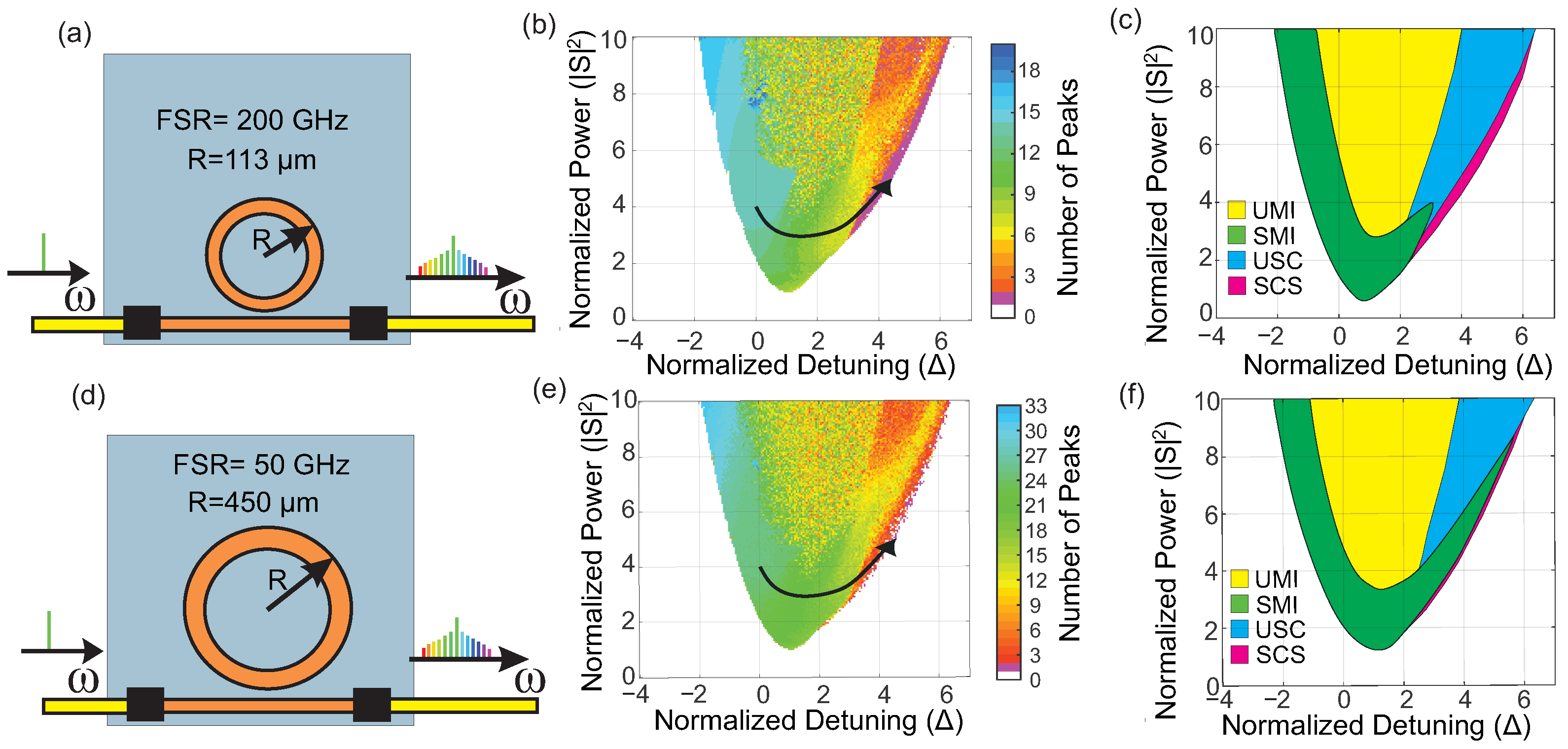
For this reason, we propose, for the microresonator with a radius of 113 µm, an anomalous dispersion , a photon lifetime ns, a Kerr coefficient , a loss coefficient , and a coupling coefficient . For the microresonator with a radius of 450 µm, we propose , ns, , , and a coupling coefficient . We select these parameters because they allow us to generate stable optical frequency combs with paths that facilitate reliable generation. These parameters can easily integrate the proposed devices with other photonic components to form a compact, low-cost optical comb generator.
To identify the paths of generation, a description of the parametric space
is required, as proposed in [
42]. This method uses the Lugiato–Lefever Equation (LLE) to perform various simulations and verify the final state of the generated spectrum. We choose this approach because it allows us to observe in detail the propagation of the electromagnetic field in the microresonator as we vary the input laser parameters. The LLE equation is defined as
where
is the complex envelope of the total intracavity field,
t is the time variable,
is the transverse coordinate,
is the round-trip time,
is the phase detuning,
L is the cavity length, and
is the pump field. To solve this equation numerically, we use the split-step Fourier method. It is important to emphasize that the pump power and detuning are normalized (see Equations (
2) and (
3)) to compare the results with those of other methods in the literature [
42], where
To conduct the simulations, we initiate the field within the cavity in the frequency domain
using complex Gaussian noise with a standard deviation of
. Subsequently, we set the initial state
and maintain this state for a duration of 1.5 µm. After this, we transition to a final state
and we hold this state for another 1.5 µs. We repeat this process for different final states and reconstruct the parameter space as proposed in [
42]. A single soliton or dissipative Kerr soliton (DKS) is chosen as the final state because the frequency comb contains the largest number of optical carriers, which is essential for our method. For the 200 GHz MRR, we set
, and, for the 50 GHz MRR, we set
.
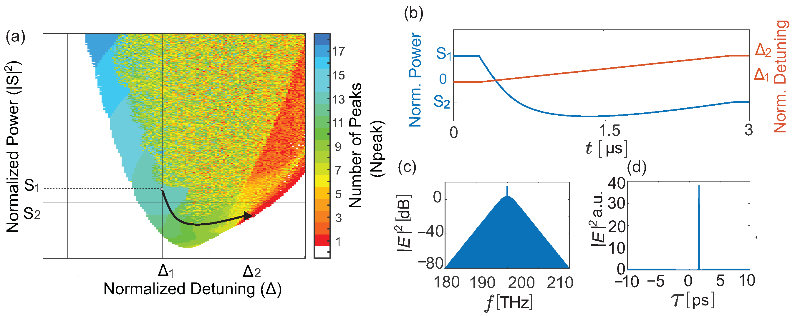
We generate a stable OFC by varying the parameters
using a path obtained from the parameter space. We select a detuning value of
as the starting point, and the parameters are varied until reaching a final point in the region of DKS in the lower-right part of the parameter space
. This choice is justified because this comb type exhibits more significant wavelengths with high coherence and stability.
Figure 4b shows the path in blue and orange. We establish a non-linear power variation to avoid the chaotic region, as mentioned in [
42].
We verify the probability of generating a DKS with the established paths. We carry out this process because the paths do not always produce the same type of OFC, and we need to adopt a deterministic approach. We perform multiple simulations using the LLE equation with the established path to verify the probability of DKS generation. During each simulation, we count the number of pulses appearing in the microresonator at the end of the process. If only one pulse occurs, DKS generation is considered successful. We repeat this process for each simulation and generate a histogram that shows the number of pulses obtained during 200 repetitions. This result allows for the evaluation of the proposed path’s suitability or the need to offer alternative means to achieve the goal of deterministic generation. We select the path with the highest probability of generating a single pulse based on the obtained histogram.
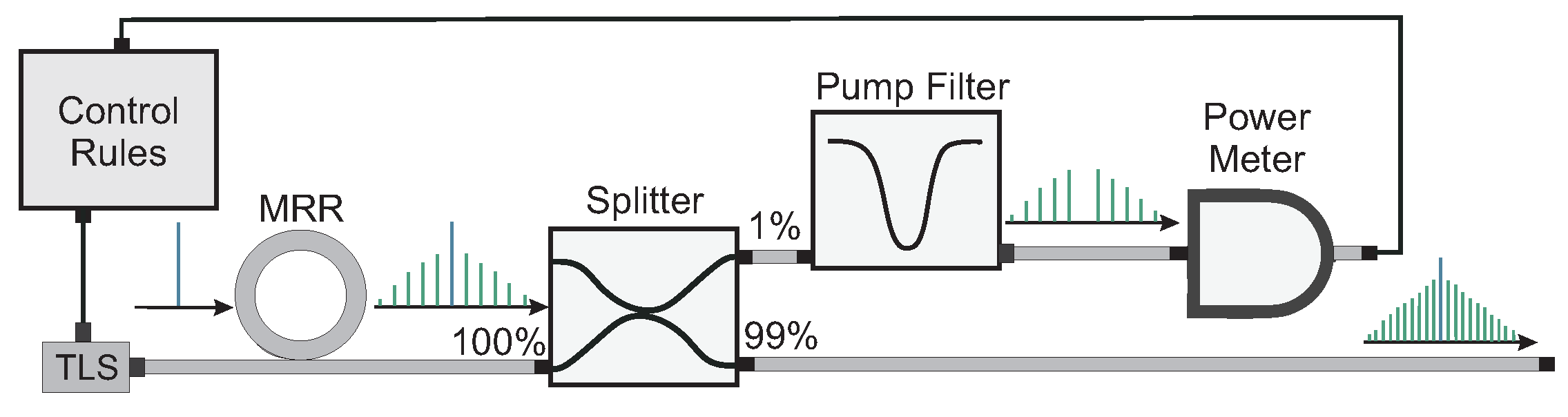
Obtaining DKS in optical microresonators is a complex process requiring a control strategy to achieve a single soliton state. Therefore, we propose the scheme illustrated in
Figure 5 to overcome this challenge. In this proposal, we generate an OFC and subsequently employ a splitter to obtain the minimum fraction of the optical wave (1%) to verify the attainment of the DKS state. To validate the DKS state, we filter the signal with a reject band at the central frequency (1.55 µm) and measure the power using an optical detector. If the power falls within a specific range, we conclude that we have generated the soliton; otherwise, we must repeat the generation process until we achieve the desired state. As we base our methodology on simulations rather than physical experiments, we use the intracavity power as an analog measure of the power measured by the optical detector. The power spectral density measures the energy accumulated within the MRR, indicating the presence of the DKS. With this strategy, we can validate the methodology without losing generality in the proposal. In our simulations, the ranges of intracavity power for the verification of the generation of the DKS are
and
a.u., for 50 GHz and 200 GHz MRR, respectively. This ranges should be adjusted experimentally by taking into account all the optical losses from the MRR to the detector and analyzing the soliton steps.
2.4. Optical Scheme for Multiple Customer Assignments Using Optical Combs
To assign the spectrum in this solution, we propose using a passive optical network that employs wavelength division multiplexing to transmit digital information across multiple channels. In this network topology, we utilize a programmable line-by-line pulse shaper to assign the spectrum generated by the optical microresonators and to obtain the wavelengths used in modulation [
43,
44]. A pulse shaper is an optical device that controls the phase and amplitude of a light wave. This device consists of three key elements. First, there is a diffraction grating whose primary function is to separate the light pulse into its different constituent wavelengths. The second component is an optical modulator, critical in allowing programmable adjustments of each spectral component’s amplitude, phase, and polarization. In a more detailed context, known as “line-by-line”, this modulator can finely tune each spectral line in a specific manner. As the final component, an inverse diffraction grating is employed to reconstruct the spectral components that have been modified, thus forming the final light pulse. It can work with one or multiple light waves at its input, which makes it adaptable to various needs requiring waves with different spectral properties. Additionally, this device can have one or multiple outputs, allowing for the light wave to be redirected toward different directions or to separate different portions of the spectrum of a light wave for various communication channels. Moreover, it can divide the input power into several outputs, which is helpful in applications requiring precise and efficient wave distribution. This device is electronically controlled, enabling the real-time adjustment of assignments algorithmically.
For this study, the pulse shaper selects from four optical combs with separations of 12.5 GHz, 50 GHz, 100 GHz, and 200 GHz. The pulse shaper assigns the spectrum of each comb according to instructions from the RMLSA algorithm. Each wavelength is then fed into a QAM multi-level modulator, and the modulation level is determined using the RMLSA method based on the required distance and requested bandwidth. Subsequently, the modulated waves are combined using an interleaver for transmission over a single fiber channel. In the reception stage, another pulse shaper separates the spectrum again according to the previous assignment and performs the demodulation process.
Figure 6 shows the network topology. Notably, the pulse shaper can assign either a single wavelength from the comb or a range of wavelengths in the case of a super-channel, thus enabling the generation of a flexible grid, which is fundamental in our methodology.
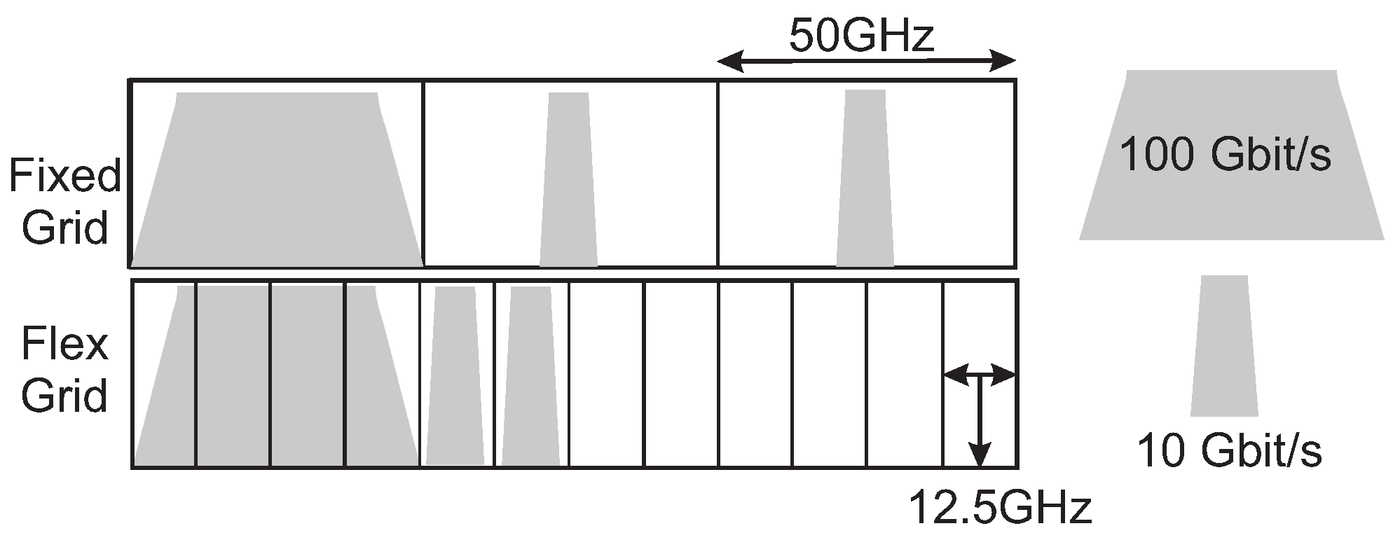
2.5. Method for Spectrum Assignment Using Multi-Level Formats and Optical Frequency Combs—RMLSA
In this application, we design an RMLSA algorithm to control the pulse shaper based on the bandwidth and distance information of each request in the network, to find an appropriate optical comb carrier for the transmission process. In designing this algorithm, we propose a heuristic methodology that efficiently assigns wavelengths while respecting several constraints. These constraints include the request-required transmission distance, the transmission distance of the wavelength based on its modulation configuration, and the number of lines needed per modulation. Furthermore, we ensure that the assigned super-channels are contiguous and adjacent, without any gaps. The primary goal of this allocation is to optimize the spectrum. Our algorithm employs a flexible grid ranging from [12.5, 200] GHz to select the modulation format that requires the smallest spectrum region while ensuring that the format can transmit at the required distance. This grid structure allows for the flexible allocation of resources. It enhances the spectrum efficiency by assigning small bandwidths on small grids or utilizing all spectrum wavelengths when creating a super-channel for a large bandwidth requirement. To illustrate this,
Figure 7 depicts the spectrum organization on both rigid and flexible grids, as proposed by our algorithm.
Some strategies for spectrum allocation have been proposed. However, these strategies are unsuitable for MRR use, and some entail high computational costs. Therefore, we propose the spectrum allocation algorithm depicted in Algorithm 1. This algorithm maximizes the utilization of network resources, specifically comb lines, while minimizing the number of rejected requests. Firstly, the algorithm calculates the bandwidth matrix (
) and the matrix of required carrier counts for each modulation format (
) for each bandwidth request. Then, it determines the necessary OSNR for each modulation format to achieve a desired bit error rate (BER) and computes the distance at which each request can be placed on the optical comb when considering fiber attenuation.
| Algorithm 1 RMSLA Assignment Algorithm for OFCs. |
| 1: | ▹ Fiber attenuation in dB/km |
| 2: | ▹ Communication BER |
| 3: | ▹ ith modulation used |
| 4: | ▹ OFC free spectral range |
| 5: | ▹ jth request bandwidth |
| 6: | ▹ jth request distance |
| 7: | ▹ Optical comb spectrum in [dB] |
| 8: | ▹ OSNR for tmod [i] |
| 9: | ▹ Assignment vector with each demand |
| 10: | ▹ Rejection vector |
| 11: |
| 12: | ▹ Number of modulation formats |
| 13: | ▹ Request number |
| 14: | ▹ Comb line number |
| 15: for to do | |
| 16: for to do | |
| 17: | ▹ Compute bandwidth for tmod[i] modulation |
| 18: | ▹ Compute carrier number |
| 19: if then | ▹ Check if VL is odd or even |
| 20: | ▹ If even, the algorithm requires a longer wavelength |
| 21: for to do | |
| 22: | ▹ Compute OSNR for a modulation format |
| 23: for to do | |
| 24: | ▹ Vector of distances for each comb line |
| 25: | ▹ Compute distance for each tmod[i] |
| 26: | ▹ Cost equation for each demand |
| 27: | ▹ Sort in descending order of cost |
| 28: | ▹ Organize bandwidth based on VP ordering |
| 29: | ▹ Organize distances based on VP ordering |
| 30: | ▹ Matrix of required lines ordered by VP |
| 31: for
do | |
| 32: | |
| 33: for do | ▹ Search from the highest to the lowest modulation format |
| 34: | ▹ Assign 1 to distances > i-th demand |
| 35: if then | ▹ If found lines are greater or equal than required proceed |
| 36: | ▹ Find the group of contiguous lines as a candidate for assignment |
| 37: | ▹ Compute the size of candidate groups |
| 38: for do | |
| 39: | ▹ Select candidate group |
| 40: if then | ▹ Check if group has enough lines to assign |
| 41: | ▹ Counter for groups with sufficient lines for assignment |
| 42: for do | |
| 43: | ▹ Assign ibd[i] to VA positions for each group |
| 44: | ▹ Fill used lines with zeros to exclude them |
| 45: | ▹ Stop iteration when demand ibd[i] is assigned |
| 46: | ▹ Stop iteration when all groups have been analyzed |
| 47: if then | ▹ If no group was assigned, add rejected request |
| 48: | |
| 49: | ▹ Store rejected demand ibd[i] |
| 50: |
| 51: function | ▹ Compute OSNR for a modulation format |
| 52: function | ▹ Compute the wavelength contiguous group in VA vector |
Next, it sorts the requests in descending order based on a cost equation considering the bandwidth and distance, to prioritize more complex requests. The sorted requests are then processed in order of decreasing cost, searching for the optical comb carrier that can satisfy each request. The arrays ( and ) are searched in decreasing order of modulation level, since higher levels require less bandwidth and enable better resource utilization. If sufficient consecutive lines are available, they are assigned to the request and marked as unavailable for other requests. Otherwise, the request is marked as rejected. We use several auxiliary functions to perform these tasks, including a function to calculate the required bandwidth for each modulation format, a function to determine the required carrier count according to the bandwidth and modulation format, a function to compute the OSNR required for a given BER, and a function to verify the available and contiguous wavelengths on the optical comb.
2.6. Validation Phase
To validate the functionality of the network structure and ensure the proper allocation of network requests, we propose the following process. In this study, we conduct a repeatability analysis to assess the likelihood of soliton generation along a specific path. We replicate the soliton generation process 200 times to achieve this objective by utilizing distinct initial field values. These initial values are obtained by applying complex Gaussian noise with a standard deviation of
. Subsequently, we examine the final state of the path for each repetition to verify the formation of DKS. The experiment involves counting the number of peaks obtained in the field intensity and confirming the successful generation of the comb. The results from each repetition are recorded in a histogram, enabling a thorough analysis of the path [
42]. Additionally, we conduct a Monte Carlo experiment to determine the accuracy percentage in classifying the required optical comb type in a set of network requests. To achieve this, we randomly obtain 70% of the data for training and 30% for testing to quantify the results. Using the test data, we compute the confusion matrix for the SVM classifier and compare its performance with that of other popular methodologies in the literature. We calculate the average behavior and standard deviation from the confusion matrices obtained in each simulation.
We calculate the number of rejections against the number of customers and the required bandwidth to observe the network scope and identify the variables that increase rejections in requests. We also compute the amount of bandwidth assigned in the
n requests and the bandwidth blocking ratio (see Equation (
4)):
Here, is the total bandwidth rejected, and is the total bandwidth of the requests. These metrics allow us to verify the network’s performance. Finally, we propose two state-of-the-art methods to compare their performance with that of our methodology; these methods are First-Fit (FF) and Random Wavelength Assignment (RWA).
3. Results and Discussion
In this section, we present the results obtained from validating the performance of the proposed method in this research.
Figure 6 illustrates the characterization of the parameter space
for rings with an FSR of 200 GHz and 50 GHz. Note that the lower-right portion (SCS) shows the region with optical combs that exhibit a larger number of spectral lines (DKS), and we identify it in magenta. We propose a non-linear path design in [
42] to avoid the chaotic region and enable reliable comb generation due to the difficulty of generating this comb type.
Figure 8a,e show the proposed paths in black. It is important to note that the MRR in
Figure 8a facilitates DKS generation by possessing a zone with higher amplitude. In contrast, the MRR in
Figure 8d demonstrates the less frequent appearance of these states, indicating that their generation poses a difficulty for this geometry.
To estimate the functions that describe the dynamics of the proposed paths, we utilize the curve-fitting tool and estimate models of Equations (
5) and (
6) using data from the parameter spaces
. The path proposed for the MRR shown in
Figure 8a is defined by Equation (
3), while the path for the MRR shown in
Figure 8b is defined by Equation (
4).
linearly varies in the range [0, 5.219] and [0, 5.4105] for the 50 GHz and 200 GHz MRR, respectively.
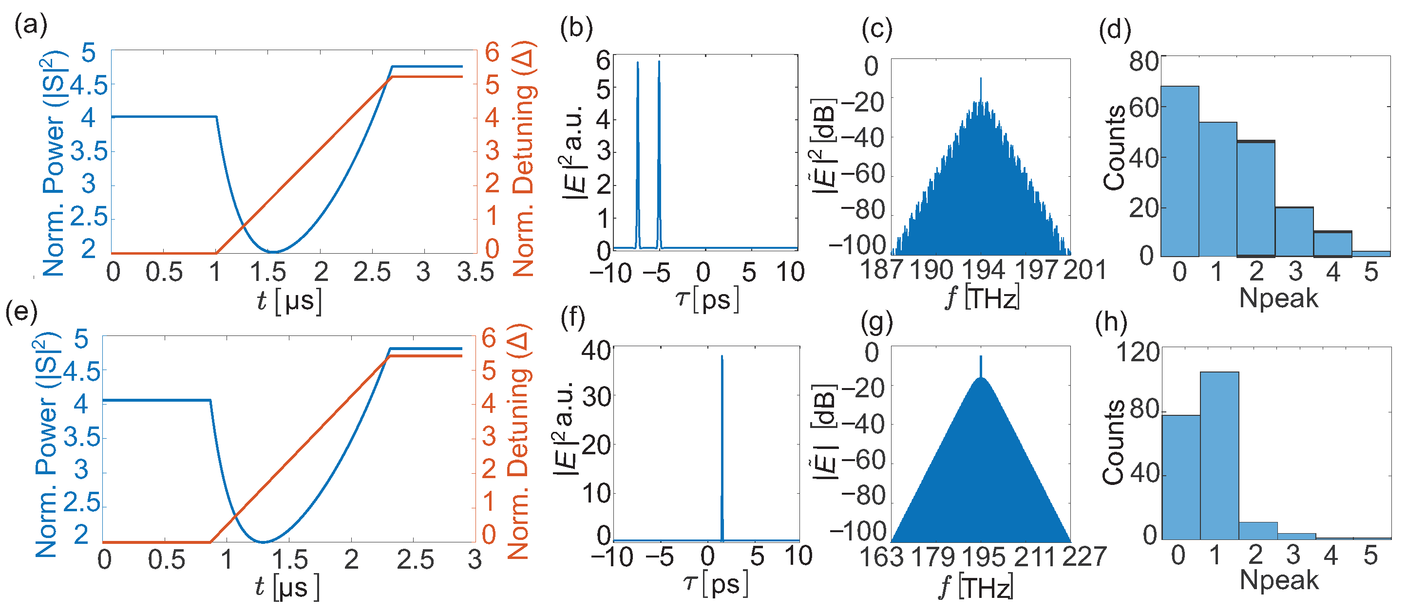
After calculating the paths, we perform a Monte Carlo experiment to assess the variability in generating these paths for each MRR without the control rule. This experiment randomly varies the initial state of the field by introducing E(w) as a complex Gaussian and verifies the achievement of the DKS.
Figure 9 shows the results of the Monte Carlo experiment, where frequency combs ranging from 1 to 5 pulses are obtained over 200 repetitions, regardless of the variation in noise introduced in the simulation (see
Figure 9d,h). DKS generation exhibits probabilistic behavior since every simulation does not achieve it. Despite this result, the DKS appears with a probability greater than 50% for the 50 GHz and 200 GHz MRR, respectively. The significance of these results is that the control strategy can quickly generate the state by repeating the generation a finite number of times.
Upon characterizing the paths, the control strategy implements the generation process. This process exploits the DKS appearance probability to achieve a state with minimal repetitions.
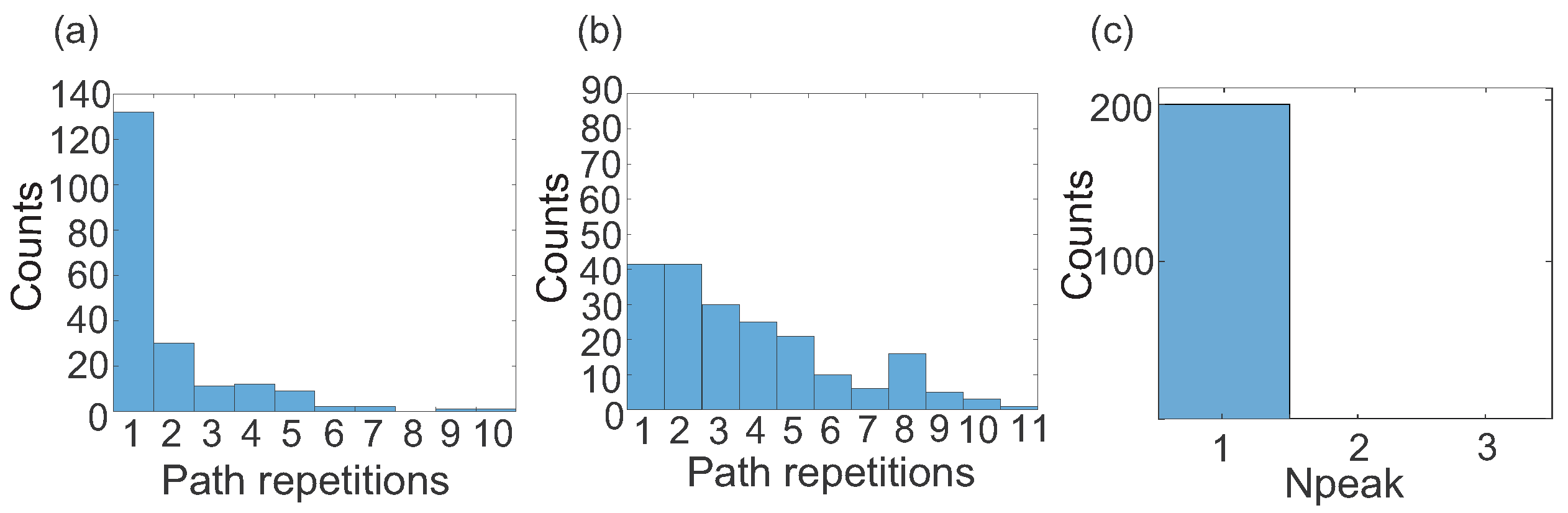
Figure 10c shows that 200 Monte Carlo experiment simulations always yield the DKS state. This outcome is crucial as it ensures deterministic generation, which is the primary goal of this strategy.
Figure 10a,c show the repetition frequency of the generation through the control strategy. The generation through the control strategy produces the soliton state between 1 and 11 repetitions. This finding is significant because it does not require many repetitions to achieve the desired state, indicating a time range between 3 and 37 µs for this generation, which is appropriate for these communication systems.
With the deterministic generation of frequency combs, we validate the machine learning system that classifies the required comb type to attend to network requests. The results of the Monte Carlo experiment performed in this work are presented in
Table 3, which shows the confusion matrix diagonals that correspond to the accuracy percentages of each of the studied classification methods. Note that the SVM method efficiently classifies the four types of combs with accuracy percentages greater than 97%. The result of this classification indicates that the method can reliably identify the required comb type for the network. Additionally, other classification methods show statistically similar performance to that evidenced by the SVM, indicating that the computed characteristics appropriately describe the separation space. We choose the SVM as the approach for classification due to its lower computational cost, which is a fundamental factor in carrying out dynamic spectrum assignment. Regarding these results, the classification error of approximately 3% can be ascribed to various factors. Firstly, specific application scenarios inherently pose complexities in classification due to their distinctiveness and resemblance to adjacent classes. Furthermore, data noise also contributes to this margin of error. Lastly, inherent limitations within the chosen model’s architecture may affect its capacity to confront the data’s challenges. The amalgamation of these factors leads to the observed 3% error and emphasizes the significance of exploring novel classification model proposals. Note that CNNs exhibit poorer performance than classical learning methods. This result arises due to the database’s tabular nature, making it challenging for CNNs to adapt as effectively as classical methods to such scenarios [
40]. We can observe that the CNN model is over-fitted. This issue is attributed to the tabular feature and the insufficient data in the database, rendering it unsuitable for deep learning approaches.
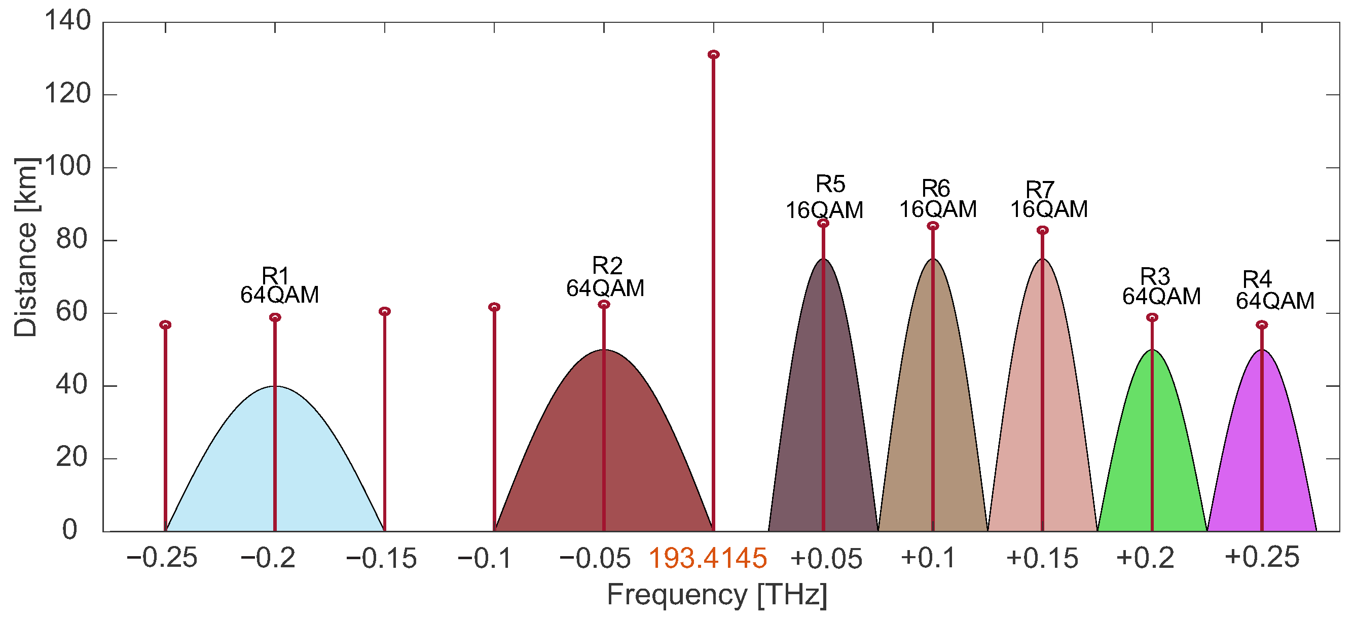
For the validation phase of the allocation algorithm, we propose a scenario that includes eleven wavelengths of an OFC with an FSR of 50 GHz and seven requests. This experiment aims to improve our understanding of the allocation process and algorithm functioning. In order to assign lines, we propose using a multi-level quadrature amplitude modulation (QAM) format, which allows for modulation levels of 16, 32, and 64, thereby ensuring the attainment of varying bandwidth levels within the limitations of distance. The first user (R1) requests 450 Gbit/s at 40 km; the second user (R2) requests 200 Gbit/s at 50 km; the third user (R3) requests 100 Gbit/s at 50 km; and the fourth (R4), fifth (R5), sixth (R6), and seventh (R7) users request 50 Gbit/s at distances of 50 km and 75 km.
Figure 11 shows the OFC wavelengths, their kilometer capacities, and the results of spectrum assignment for the requests. Note that our method assigns each request in a modulation format that guarantees the minimum transmission distance. Furthermore, note that requests 1 and 2 use super-channels to support modulation. This result verifies that the algorithm responds to the ideas proposed for the assignment.
Subsequently, we propose an experiment with 1400 request scenarios based on the variations in
Table 1. The goal of this experiment is to compute the performance of the proposed method. To carry out the assignment, we employ an SVM to select the appropriate OFC and apply the proposed RMLSA algorithm. These request scenarios can simultaneously accommodate up to 200 requests, with a maximum bandwidth of 31 THz.
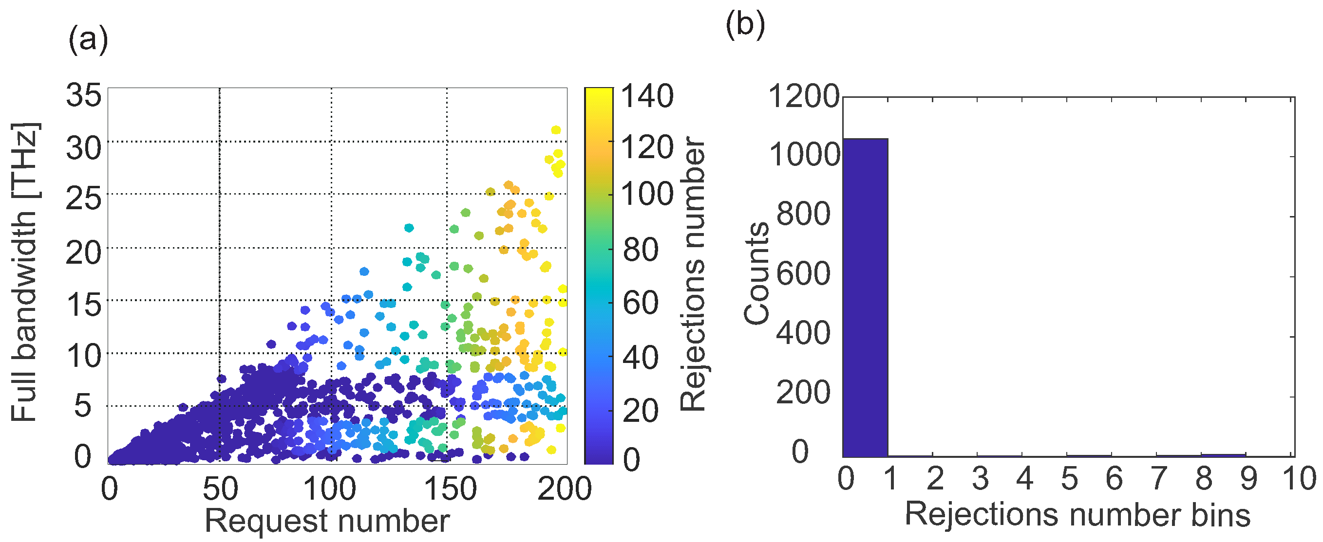
Figure 12 displays the number of rejections obtained by the assignment algorithm. Notably, increasing the number of requests and their respective bandwidths leads to a corresponding increase in rejections (see
Figure 12a). This observation emphasizes the importance of maintaining the maximum number of available carriers to prevent these rejections. Furthermore, rejected requests are more likely to have large bandwidths because a request of such magnitude requires a super-channel, significantly reducing the number of available carriers. Despite encountering rejections during the exercise, it is important to note that the rejection number is minimal. Specifically, out of the 1400 request scenarios, 1060 could be addressed using the proposed method (see
Figure 12b). These findings imply that the proposed method is reliable when facing real-world network situations. It is important to emphasize that the allocation of users relies on three factors: the request bandwidth, the quantity of carriers accessible for assignment, and the transmission distance of each user. Bandwidth demands may necessitate a substantial quantity of carriers to construct a super-channel, consequently diminishing the pool of carriers available for other users. Moreover, not all carriers can meet quality of service (QoS) requirements due to the sech2 profile of the frequency comb. Consequently, when customers are situated at significantly extended distances, the likelihood of their requests encountering rejection elevates. Hence, maximizing the amount of available spectral components is imperative to enhance the network allocation performance.
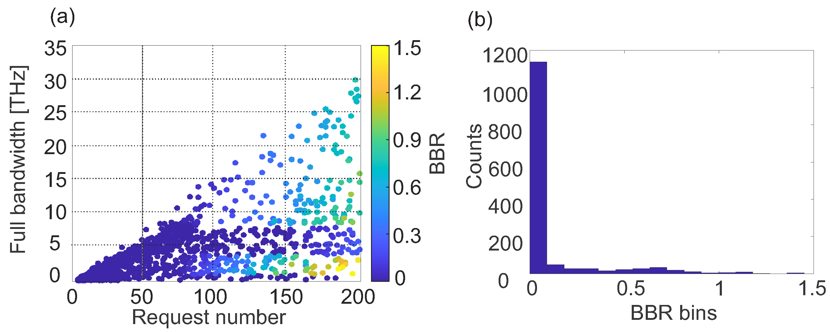
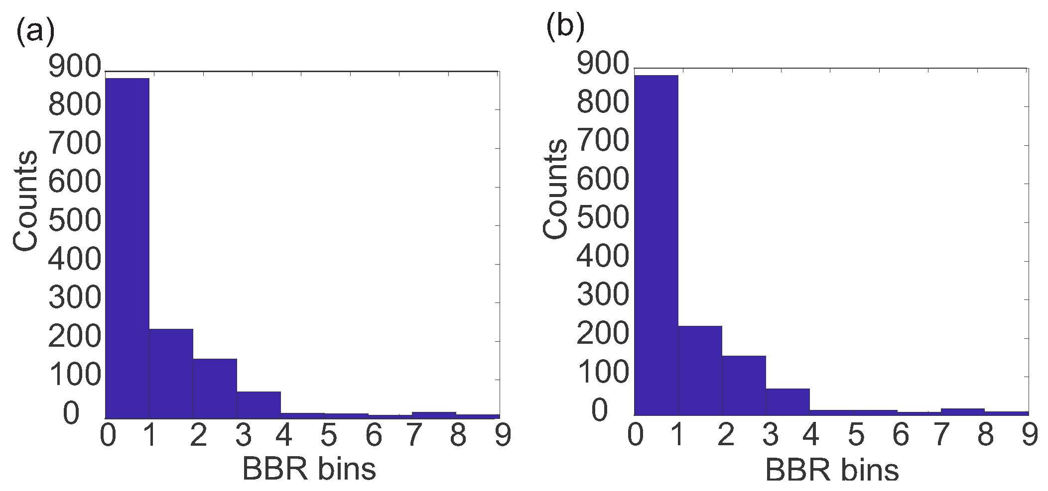
Another important metric to measure network efficiency is BBR; this metric quantifies the likelihood of the network being blocked due to a bandwidth that exceeds the assignable limit.
Figure 13a shows the BBR calculation for each network request. As with the previous figures, there is a higher probability of blocking when requests with many customers and large bandwidths exist. However,
Figure 13b shows that our method successfully addresses 1090 requests with a blocking probability of zero, accounting for 81% of the total requests. This result demonstrates that our method exhibits adequate adaptability to this type of demand.
To compare our methodology with other state-of-the-art approaches, we implement the FF and RWA methods [
41,
45] in a WDM scenario. These methods operate with a fixed number of wavelengths and attempt to minimize the blocking probability. However, the FF and RWA methods utilize multiple carriers generated from individual lasers, significantly fewer than those obtained from an optical frequency comb. This limitation occurs due to the cost of implementing the network, which increases with the number of lasers. Therefore, to allow a useful comparison with our design, we propose a scenario with 60 available carriers, which are all distributed according to the WDM-UIT proposal. In this distribution, all carriers have the same OSNR of 60 dB.
In
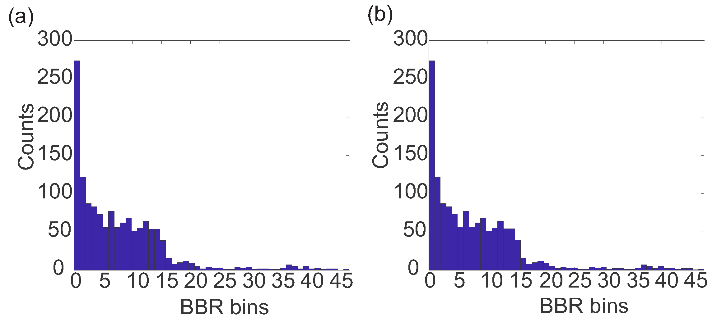
Figure 14, we can observe the result of computing the histogram for the calculation of BBR. We can observe that our method has a lower blocking probability compared to the FF and RWA methods. To verify this observation, we count the number of requests with a blocking probability greater than 0%, likely to have not been assigned, or to have a low probability of assignment. It is worth noting that the FF method has 518 requests with a blocking probability greater than 0%, and the RWA method has 519 requests with a probability greater than 0%, whereas our method has 310 requests. On the other hand, these methods show greater variability in the experiment, indicating that their blocking probability is higher for some scenarios, reaching values of up to 9%, resulting in inadequate network performance. This problem arises because our approach can use a more significant number of carriers and take advantage of the lines generated by the optical frequency comb. Our method allows for a reduction in the blocking probability and better adaptation to the proposed scenario. It is important to note that these methods can exhibit cases of blocking probability up to 8%, whereas our method only exhibits up to 1.5% probability.
Although the percentage of unblocked requests is close to that in our method, the methodology proposed in this work only requires eight lasers to achieve this performance, which significantly reduces the implementation costs. This laser number is a fundamental factor because this device is one of the most expensive and complex in the network. Another test proposed to measure performance is to use the same number of lasers used by our approach for the FF and RWA methods, thus verifying the blocking probability. Note that the network performance drops significantly, obtaining 1126 requests with a blocking probability higher than zero for the FF method and 1129 requests for the RWA method (see
Figure 15). This result justifies the clear advantage that our method has over these approaches. On the other hand, in some situations, the probability of blocking can reach up to 45%, which is excessively high for a network.
Our RMLSA approach demonstrates an execution time of ms in the context of 200 request assignments. In contrast, the First-Fit method exhibits an execution time of ms, while the Random Wavelength Assignment method records an execution time of ms. Notably, the RMLSA approach proves to be competitive compared to established methodologies in the state of the art. Furthermore, we are exploring hardware acceleration approaches to enhance the algorithm’s performance.
4. Conclusions
This paper presents a methodology for the implementation of a PON network with dynamic spectrum allocation and an RMSLA-WDM approach. This method allows for the use of frequency combs generated by MRRs and provides an optical source with multiple carriers and a different ONSR, which enables the use of the WDM technique for customer assignment based on the distance requirements of their geographic locations. This solution reduces the costs of these networks, using only eight lasers to achieve a flexible WDM grid. Moreover, our method allows for the assignment of a significant number of carriers by utilizing multiple MRRs, which helps to achieve the performance presented in this work. The use of MRRs helps to improve grid tuning as their carriers have high phase coherence, a factor that is difficult to achieve with individual lasers.
On the other hand, we establish a reliable strategy for the generation of frequency combs with an adequate number of carriers using silicon nitride (SiN) MRRs with a radius of 113 µm and 450 µm. These paths allow us to obtain frequency combs with an FSR of 50 and 200 GHz. Thanks to the thermal control strategy and multiple MRRs, we generate smaller FSRs with more lines, allowing for FSRs of 12.5 GHz, 50 GHz, 100 GHz, and 200 GHz. We also design an RMSLA-WDM dynamic spectrum allocation algorithm that considers multi-level modulation formats such as QAM and carrier allocation with the optimization factor of using the smallest number of lines that can meet the transmission distance given by their OSNR. The proposed allocation algorithm in this work adapts to the dynamics of a network with 200 customers and variable bandwidths, making it a potential solution to the current needs in this field.
The ONSR in the OFC plays a significant role in the efficiency and range of communication systems based on WDM and QAM. Reducing the noise level in the spectral components of the OFC becomes a critical factor in maximizing the performance of this approach. This is because reducing the noise allows for each transmitted wavelength to reach a greater distance and also enables more useful spectral components in the frequency comb. For successful future implementation, it is essential to address this challenge by employing optical techniques that minimize the noise in the frequency comb after its generation on the optical chip. This strategy will maximize the transmission capacity and range of communication systems, providing an effective and high-performance solution in optical communications. In future work, we propose using dual coupled microresonators to achieve deterministic soliton generation. This outcome will enable the maximization of the available carriers and a reduction in laser tuning time during the process. Additionally, we will experimentally validate our methodology by physically implementing all of its components.
The dynamic spectrum allocation using optical frequency combs proposed in this paper has immense potential for quantum networking and communications. These devices enable the precise and controllable generation of multiple optical frequencies, facilitating the multiplexing of quantum signals at different wavelengths. This dynamic optical frequency allocation capability optimizes spectrum utilization and spectral efficiency in quantum networks while ensuring enhanced security in quantum information transmission by rendering unauthorized access even more challenging. Furthermore, optical microresonators offer high-frequency coherence and stability, which are essential factors in maintaining the integrity of the quantum properties of the transmitted states. In summary, this technology has the potential to enhance the scalability and performance of quantum networks by offering significant advantages in terms of speed, security, and quantum communication capacity [
46,
47,
48].


