
On the Magnetic Properties of Construction Materials for Magnetic Observatories
by
 , , , and
Roman Krasnoperov
1,
Roman Sidorov
1,* ,
,
Andrew Grudnev
1,
Jon Karapetyan
1,2 and
and
Dmitry Lazarev
1 1
Geophysical Center of the Russian Academy of Sciences (GC RAS), Moscow 119296, Russia
2
A. Nazarov Institute of Geophysics and Engineering Seismology of the National Academy of Sciences of Republic of Armenia (IGES NAS RA), Gyumri 3115, Armenia
*
Author to whom correspondence should be addressed.
Appl. Sci. 2023, 13(4), 2246; https://0-doi-org.brum.beds.ac.uk/10.3390/app13042246
Submission received: 25 December 2022
/
Revised: 3 February 2023
/
Accepted: 4 February 2023
/
Published: 9 February 2023
(This article belongs to the Special Issue Ground-Based Geomagnetic Observations: Techniques, Instruments and Scientific Outcomes)
Abstract
:The installation and development of a magnetic observatory can require additional studies of the magnetic properties of construction materials for pavilions and measurement pillars, as well as of the environmental conditions, including, first of all, the magnetic properties of the surrounding rocks. In some cases, detailed studies of magnetic susceptibility can be necessary. To date, these procedures have only briefly been described in the existing manuals and guides. With the development of new construction materials, as well as with the increase in the number of magnetic observatories, the need for such studies has risen even more. This article is focused on studies of the magnetic properties of construction materials for magnetic observatories, and the results are presented based on our experience in the deployment of magnetic observatories and stations in Russia and abroad. An overview of the magnetic susceptibility of different materials is presented. A kappametry method and its application to studies of construction materials are described, and the results of magnetic susceptibility tests performed on the construction materials and the surrounding rocks in the vicinity of an observatory are provided. Finally, some recommendations for studies of materials for observatory construction are given.
1. Introduction
A geomagnetic observatory is a complex facility that carries out precise measurements of the components of Earth’s magnetic field on a regular basis. The creation of and support for such posts that carry out continuous measurements of the elements of Earth’s magnetic field have long been relevant due to the constant need for geomagnetic data, which are used in numerous studies of fundamental and applied research in the Earth sciences and solar–terrestrial relations [1]. The installation of a geomagnetic observatory is a sequential multi-step task, which includes the selection of a suitable location, the study of the geomagnetic anomalies from geological or artificial near-surface sources [2], the determination of sites for the construction of a magnetic pavilion and the installation of an azimuth mark for absolute measurements, the selection of non-magnetic construction materials for pavilions, the design of communication and power supply networks, the selection of heating devices and temperature stabilization systems, and so on.
During collaborations of scientific institutions on the deployment of geomagnetic observatories, several guidelines were developed [3,4], and these provide fairly comprehensive coverage of the mentioned issues. However, they describe only general rules and recommendations for deploying magnetic observatories, and many comment factors always affect the installation progress of each individual observatory. In particular, the conditions of the location of an observatory are different in different environments. In regions with cold continental or polar climates, the proper temperature stabilization of vector fluxgate magnetometers requires insulation of the pavilion walls and an automated heating system that compensates for seasonal temperature fluctuations, whereas, in mild climate conditions, such additional adaptations are less relevant. Another issue is the geological structure of the observatory site, the underlying rocks, and their magnetization, which contributes to lithospheric anomalies. Therefore, it is impossible to simply replicate observatories in different locations in exactly the same way. Every observatory is unique in this regard, and different observatories require different approaches for their proper functioning.
Thus, research communities and teams engaged in the deployment of magnetic observatories are free to make independent choices and apply any technical solutions for proper equipment within the regulations and constraints listed in the guidelines. Nevertheless, at various construction stages, specific procedures and technical solutions are required, and these take local settings and instrumentation into account. For example, in the Geophysical Center of the Russian Academy of Sciences (GC RAS), a specific methodology was developed for geophysical studies with the aim of searching for suitable magnetic observatory locations by using modern GNSS technologies [2]. Next, some cheaper solutions were found for the heating and thermal stabilization of measurement pavilions [5], such as replacements for non-magnetic copper or ceramic heaters. Finally, in recent years, various non-magnetic composite materials that can be used in observatory pavilions have been introduced into construction practice. These new materials should be characterized from the magnetic point of view to ensure that they do not introduce magnetic anomalies.
Measurements of the magnetic susceptibility of rocks that are conducted either in situ or in the laboratory provide information for various studies in the areas of geology, archaeology, technical geophysical tasks, etc. However, there have not been very many studies that have provided detailed descriptions and application examples in the framework of magnetic observatory construction and maintenance. Despite there being some magnetic susceptibility studies of soils at observatory sites [6], there are still no detailed examples of studies of the magnetic properties of construction materials that were measured before an observatory’s construction.
This article focuses on the magnetic characterization of construction materials for magnetic observatories. We present an overview of the characteristics of materials, chiefly their magnetic susceptibility, which is the main feature contributing to the effects of materials and minerals in the Earth’s magnetic field. This is a summary of our experience in the deployment of magnetic observatories and stations [1]. In the future, some manuals can be prepared based on these measurements in order to demonstrate the characteristic features of construction materials, as well as some surrounding rocks. We briefly describe the kappametry method, its physical basis, and common devices used for magnetic susceptibility measurements. Next, we provide the results of magnetic susceptibility tests performed on construction materials and the surrounding rocks in the vicinity of an observatory. In addition, some recommendations on the construction of observatory pavilions will be formulated in the Conclusions section.
2. Materials and Methods
2.1. Magnetic Susceptibility and Its Measurement: Physical Basis
The magnetization of a physical body induced by an external magnetic field is a vector quantity that represents the magnetic moment per unit of volume [7]. The magnetic properties of matter are determined by the structure of atomic orbits and the magnetic moments of the electrons. It is well known that the main magnetic property of the substance itself is its ability to acquire a magnetization in an applied magnetic field—the magnetic susceptibility (we use κ for it as a common designation in geomagnetic research practice). Mathematically, κ is a dimensionless quantity representing the coefficient of proportionality between the intensity of the inductive magnetization and the intensity of the external (magnetizing) field. In magnetic prospecting practice, magnetization is used as a parameter that indicates the material (mineral) composition of a rock.
The magnetic susceptibility of rocks varies widely from 0 to 10 SI units. In the magnetic survey practice, magnetic susceptibility is measured in 10−5 SI units. According to their magnetic properties, all substances are divided into three groups: diamagnets, paramagnets, and ferromagnets, differing in magnetic susceptibility range and sign. The magnetic susceptibility of diamagnets is very low and is about 10−5 SI. It is negative, as the magnetization vector within diamagnets is directed against the external magnetizing field). Many minerals, such as quartz, rock salt, graphite, gold, silver, lead, copper, and rocks, such as marble, are diamagnetic. Paramagnetic substances are also characterized by low magnetic susceptibility. Most sedimentary, igneous, and metamorphic rocks contain paramagnetic minerals. Ferromagnetic substances have the highest magnetic susceptibility (up to several SI units). The reason for this is the exchange coupling between their atomic spins. Even in the absence of an external magnetic field, the magnetic moments of all atoms of a substance are parallel to each other, forming domains, the distinguishing feature of which is remanent magnetization. An example of ferromagnets magnetite (Fe3O4), which has a very high magnetic susceptibility of about 1.5 to 80,000 × 10−5 SI units). Other examples of ferromagnetic minerals are hematite (Fe2O3), maghemite (a magnetic modification of iron oxide Fe2O3—γ-Fe2O3), titanomagnetite (Fe2TiO4), and pyrrhotite, which is a magnetic modification of iron sulfide (FenSn+1, where n = 6…11). Thus, the cause of the magnetism of rocks is their chemical composition and crystalline structure of the minerals therein, especially ferromagnetic ones.
High magnetic susceptibility values are typical for rocks containing large amounts of ferromagnetic minerals. For instance, the magnetic susceptibility of some ferruginous quartzites can reach 1–3 SI. Ferromagnetic minerals, especially magnetite, are often found in igneous rocks. Such intrusive rocks as granites and granodiorites are characterized by lower κ values due to their acidic composition. Higher κ values are typical for rocks of medium composition (diorites) and basic composition (gabbro). However, in most rocks, magnetite is an accessory mineral in the rock composition, i.e., it occurs in very small quantities and therefore does not affect the rock classification. Almost all sedimentary rocks are non-magnetic. Limestones, dolomitic limestones, and dolomites have the lowest magnetic susceptibility. Specific exceptions are possible, e.g., when sandstones or siltstones formed near the drift source contain relatively large amounts of magnetite grains and have high magnetic susceptibility values as a result.
In magnetic survey practice, minerals and rocks are often classified by their magnetization. Some useful examples of such classification were made by Bersudsky [8] and Khmelevskoy [9]. As the main focus of our research is the overview of magnetic properties of artificial substances(the construction materials), here we will use the classification by gradations from the Geophysicist’s guide [10], as it is related not only to natural but also to artificial substances. According to it, the substances are classified by κ gradations listed in Table 1.
2.2. Hardware for Magnetic Susceptibility Measurements
Magnetic susceptibility measurements, or the kappametry method (named after the symbol “κ”), can be implemented not only as a support for several geophysical methods [11] but also as a standalone geophysical method for various purposes, for example, for soil contamination studies [12,13] and archaeological surveys [14]. Many magnetic susceptibility measurement devices (kappameters), such as SatisGeo KM-7 [15], Bartington MS-2 [16], or PIMV [17], are portable and designed for both in situ measurements and for laboratorial work. These devices are based on an inductive measurement method, which implies the measurement of an inductance-related signal change in a coil when applied to a specimen, compared to the inductance-related signal of the air. This allows for evaluation of the magnetic susceptibility in the volume of a specimen.
Another group of kappameters includes indoor devices designed for laboratories. These kappameters are based on various measurement techniques [18]. In our research, we used mainly a PIMV kappameter for field and indoor measurements, although some magnetic susceptibility determinations were performed using the AGICO MFK-1FA laboratory kappameter at the Laboratory of the main geomagnetic field and petromagnetism (Schmidt Institute of Physics of the Earth of the Russian Academy of Sciences). The magnetic susceptibility sensitivity of this device is 2 × 10⁻⁸ SI.
2.3. Possibilities of the Kappamerty Method in Observatory Installation Practice
From the point of view of problems associated with observatory magnetic observations, the measurement of the magnetic susceptibility of substances is of great importance. The need for susceptibility measurements arises already at the stage of searching for the most suitable place for a magnetic observatory. Strongly magnetic rocks can produce magnetic anomalies that affect the local intensity and direction of the Earth’s magnetic field. Such effects can lead to the distortion of magnetometer data [6], requiring additional processing for correcting the influence of anomalies of geological origin. In addition to checking possible intense natural magnetic anomalies, it is also important to take into account the magnetic properties of building materials. This is required to make sure that building blocks, structures, fillers, and fasteners do not contain magnetic impurities. Otherwise, residual magnetization can cause local gradients of several nT/m in the magnetic field. This is critical for the zone in the absolute pavilion where absolute measurements are made. In this zone, the vertical and horizontal gradients of the magnetic field should, if possible, not exceed 1 nT/m [3]. The absolute measurement process includes measurements at 8 different positions for the DI sensor orientation with respect to the East, West, North, and South, and any local gradient in the vicinity of the sensor will inevitably cause spatial differences in the DI magnetometer measurements, making them inconvenient.
Moreover, a structure made of initially non-magnetic material may acquire undesirable magnetizations due to ferrimagnetic contaminations. This can happen if contaminants, including iron filings, are left over after manufacturing and processing with steel tools. Finally, contaminated concrete can acquire a magnetization during solidification, as shown in Section 3.1.2.
Nowadays, there are various modern composite materials that can be used for the construction of magnetic observatories. These materials are able to provide necessary reliability and durability if used for the construction of the frames and walls of pavilions, thermal insulation, and even the construction of pillars. Wood is the most widespread non-magnetic material used for the construction of pavilions. Both exteriors and interiors of wooden buildings should be protected from wearing out. Exterior wood is often under attack from weather impacts (temperature variations, moisture, etc.) and, therefore, should be protected with weatherproof paint. Interiors also should be protected, as they may also be subject to wear during use. The same applies to wooden pillars, which are still used in some magnetic observatories. Another material used for pillar construction is marble. However, marble is rather expensive. A cheaper alternative for pillar construction uses glass blocks joined with glue. This construction has been used at many Russian observatories, such as Paratunka (IAGA code PET) or Klimovskaya (IAGA code KLI) [5]. Nevertheless, the footing for pillars should be concrete.
There is a way to estimate the magnetic anomaly of a magnetized body by its magnetic susceptibility, mass, density, and distance from it [3]. However, this estimation is approximate, as it assumes magnetically homogeneous objects, whereas real physical bodies can contain different amounts of ferromagnetic particles. Therefore, instrumental determinations of magnetic susceptibility should be an obligatory procedure during the stage of selection of construction materials for a magnetic observatory.
3. Results
Here, we present the magnetic susceptibility measurements for some materials that can be used in magnetic observatory construction (Section 3.1), as well as some examples of underlying rocks in the vicinity of the observatory, the magnetic effect of which can be considered critical for the registered magnetic field values and manual absolute measurements (Section 3.2). We also provide an example of the effect of a magnetic field from a magnetized structure on measurements performed at a magnetic observatory (Section 3.3).
3.1. Magnetic Susceptibility of Some Construction Materials for Pavilions
3.1.1. Magnetic Susceptibility Determinations
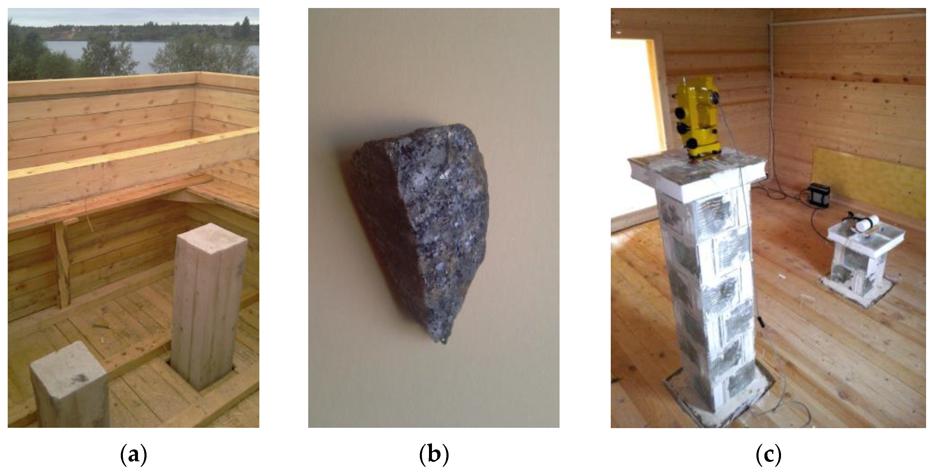
Our first experience of studying the magnetic properties of materials selected for the construction of the observatories dated back to summer 2014. In the framework of this project, it was planned to construct the observation pillars in the absolute and variation pavilions using concrete (Figure 1a). While inspecting the construction site of the future Klimovskaya observatory [5], it was found that the crushed stone selected as a filler for concrete observation pillars has a quite noticeable magnetic effect, as it was found out by a series of measurements with a GSM-19 proton Overhauser magnetometer.
Table 2 displays the anomalous geomagnetic field intensity measurements for the concrete bases at the observatory construction sites with respect to background F values (Fb). The measurements were made at 15 cm from their surface (column F15cm) and at their tops (column F0cm). As seen, the magnetic anomalies from the pillars reach 6–8 to 14–20 nT in the absolute pavilion and up to 4–5 nT in the variation pavilion, which indicates some magnetic components either in the cement or in the crushed stone.
Crushed stone samples (one of them is shown in Figure 1b) were taken from the construction site. The origin of stones is diorite, an intrusive rock that often includes hornblende; the magnetic susceptibility values for hornblende can reach 55–390 × 10−5 SI. Diorite can also contain magnetite. According to the laboratory κ determination using the MFK-1FA kappameter, κ = 120 × 10−5 SI units for the diorite sample. This value matches the low magnetizing rocks interval (see Table 1); however, such pebblestone can produce anomalous effects up to 50 nT when magnetized by an external field of about 50,000 nT (i.e., an approximate Earth’s magnetic field intensity at this region). Moreover, the cement could also contain ferromagnetic particles of artificial origin left after its manufacturing, which could also be the source of excessive magnetization. As a result of these measurements, the construction project was reworked, and the upper parts of the pillars were built from fully non-magnetic glass blocks (Figure 1c).
Another series of magnetic susceptibility measurements were performed using the PIMV portable kappameter during the development of the high-latitude White Sea (IAGA code WSE) magnetic observatory. In 2018, a location was selected for the installation of a pavilion for a single magnetometer. The pavilion is shown in Figure 2a, and its interior is displayed in Figure 2b. The pavilion walls were made of wooden boards fastened with copper nails, and for the top part of its roof, initially, an asphalt shingle sheet was planned to be used. The pillar for a POS-4 vector magnetometer (shown in Figure 2b and close-up in Figure 2c) was, similar to the previous case, built from glass bricks using glue. A concrete mix was used to form a pillar footing, and it was decided to use extended clay as a filler. A linear polyethylene tube was used as an encasement for pouring the liquid concrete mix and forming the socket of the pavilion. Thus, it was necessary to study the magnetization of the mentioned materials.
The polyethylene tube appeared to be non-magnetic (0 SI). For the concrete mix, the filler and the glue, the magnetic susceptibility measurements were carried out first directly on the materials (the kappameter was simply applied to the packages). Next, samples of each material (except for asphalt shingle (onduline) supplied in a large sheet) were taken in plastic cups for magnetic susceptibility measurements in a smaller volume. Then, 4–5 measurements were made for each material, after which the magnetic susceptibility of the samples in plastic cups was determined. When determining the magnetic susceptibility on samples with a cylindrical surface (for example, on a core), corrections must be introduced because the values on a cylindrical surface are lower than on a plane [17]. Since a plastic cup with a volume of 200 g is a cone and its diameter at one end is larger than at the other, for convenience, it was decided to choose an average correction factor from the PIMV kappameter operation manual (p. 5) for diameters corresponding to the filled part of the cup. Therefore, a coefficient of 1.4 was chosen. The measured κ values were multiplied by the mentioned correction factor. In Table 3, the column “κ, ×10−5 SI units, l.v.” contains the measurements on packing bags, and in the column “κ, ×10−5 SI units, s.v.” there are measurements of selected samples in plastic cups (“l.v.” and “s.v.” are “large volume” and “small volume”, respectively). The correction factor is 1.4. Multiplying by it the values of the magnetic susceptibility determined for the samples, we obtain values generally close to those obtained on the bags (see the column “Total κ, ×10−5 SI units”. Thus, we made sure of the purity of the experiment.
According to the results of measurements, glue (0 SI units), as well as sand concrete (9.45 × 10⁻⁵ SI units), were classified as very weakly magnetized materials. Expanded clay was weakly magnetized (127–143 × 10−5 SI units). The reason may lie in the technology of its production. However, it can still be used in the footing as a filler because it will be far from the magnetometer. The only material which had a relatively high magnetization was asphalt shingle (234–363 × 10−5 SI units, i.e., weak to medium magnetization according to the classification Table 1). Probably the asphalt shingle was contaminated by some ferromagnetic particles during its manufacturing process.
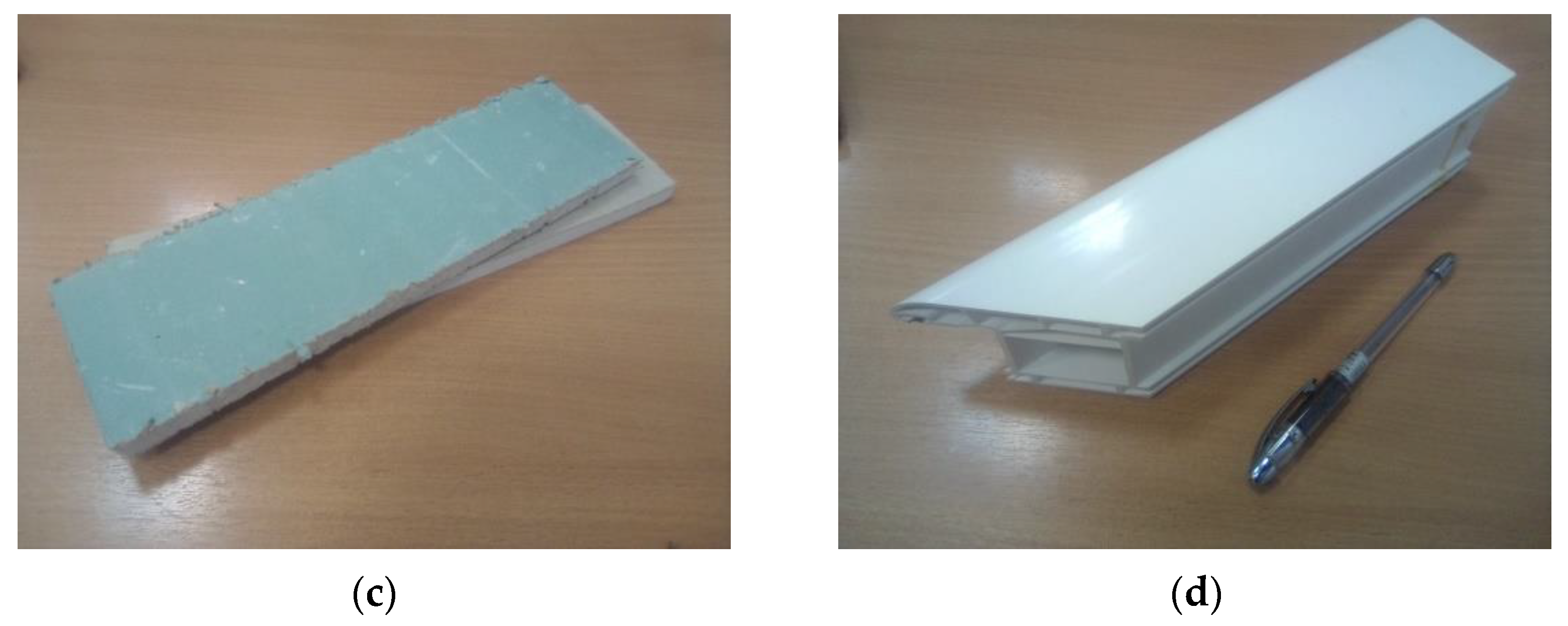
Another experience in magnetic susceptibility studies was related to the installation and development of the Gyulagarak observatory [1], IAGA code GLK, located in Armenia, in collaboration with the A. Nazarov Institute of Geophysics and Engineering Seismology of the National Academy of Sciences of the Republic of Armenia (IGES NAS RA). It was proposed to use some new composite materials for the pavilion construction and especially for the exterior finish of the pavilions, as the observatory is located in a mountain region where abrupt weather changes can take place, and wooden exteriors could soon become worn due to weather impact. Therefore, it was decided to use wood for the construction of the interiors of both absolute and variation pavilions, as well as for the construction of the inner chamber of the variation pavilion. In turn, according to the project, the frames of the pavilions were supposed to be assembled from plastic C-shape channel bars joined with aluminum rivets (Figure 3a). For the outer walls, it was planned to use plastic with polypropylene and mineral wool fill (Figure 3b) and underlying pumice blocks (Figure 3c). For window frames, we intended to use plastic profiles (Figure 3d).
The results of the magnetic susceptibility measurements of the main mentioned materials are provided in Table 4. The measurements were performed using the MFK-1FA laboratory kappameter except for a window frame profile (its magnetic susceptibility was identified using PIMV). Note that all of the specimens appeared to be practically non-magnetic.
The pillars in the observation pavilions of the Gyulagarak observatory were also built from glass blocks using glue. The κ measurements for the glue are listed in Table 5, which is similar to Table 3 for the White Sea observatory. However, in this case, the total κ values converted from the “small volume” κ values appeared to be less close to corresponding “large volume” κ values. Nevertheless, all glue samples, both loose and solid, appeared to be very low magnetizable and, therefore, suitable for pillar construction.
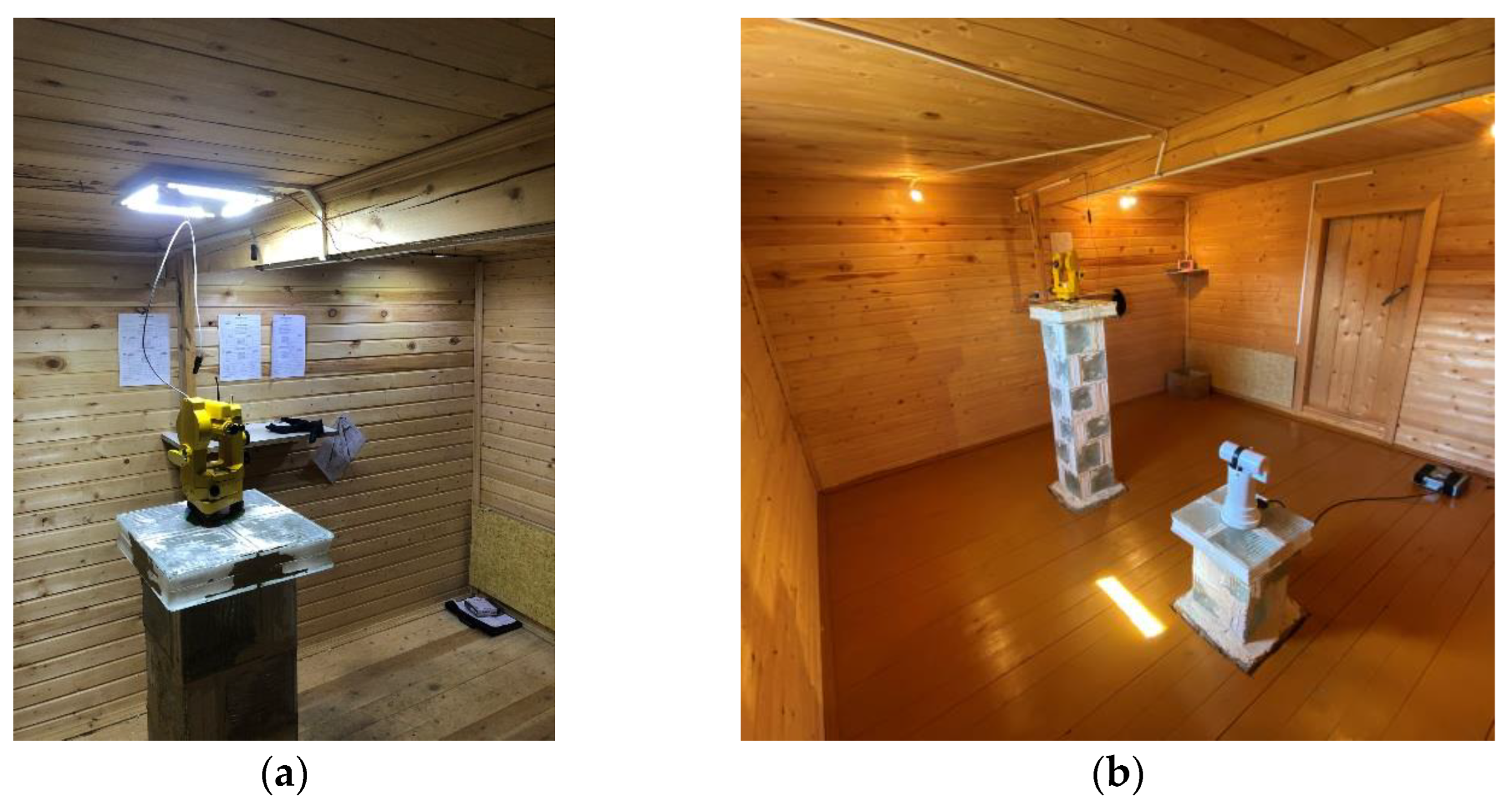
The construction process of the absolute pavilion is displayed in Figure 4a. Figure 4b shows an absolute pavilion of the GLK observatory as an example of the use of the mentioned materials, and Figure 4c shows the interior of the absolute pavilion. As seen in Figure 4c, three measurement pillars were made of glass bricks; the fourth one is experimental, and it was assembled from plastic parts. Further, we will see the advantages or disadvantages of this pillar and evaluate its stability.
3.1.2. Concrete Magnetization Due to Its Solidification
The phenomenon described in this subsection is probably the most significant challenge one has to face during magnetic observatory installation.
In terms of collaboration between the Geophysical Center of RAS and the Institute of Geosphere Dynamics of RAS, it was planned to install a full observatory set of magnetometers on the territory of the Mikhnevo geophysical observatory (Moscow region). In 2019, the place for the pavilions was selected as a result of two magnetic survey series. Later in 2019, during the development of the construction project, we made the magnetic susceptibility measurements on concrete mix samples for future pillar feet. Three series of measurements were carried out using PIMV. The resulting magnetic susceptibility values were about 7.2–7.3 × 10⁻⁵ SI, which meant that the mix belonged to very weakly magnetized building materials and was suitable for the footing construction. To avoid the magnetic effects from possible concrete mix contamination due to ferromagnetic materials or minerals, we used the same pillar design as those used at the Klimovskaya and Gyulagarak observatories (1.4–1.5 m glass block pillar mounted on a concrete monolithic part). Therefore, when the feet for pavilions were constructed, their tops were right at the floor level. In spring 2021, the pavilions were finished except for the glass parts of the pillars, and we decided to carry out a magnetic survey inside both pavilions in order to find possible sources of artificial magnetic anomalies. For this, we used the GSM-19 proton Overhauser magnetometer as a rover and another GSM-19 as a base station for diurnal correction of total field measurements. The step of the survey was 0.5 × 0.5 m. The survey was performed at two sensor height levels: the 1st level was close to the floor, and the 2nd level was 1.5 m high from the floor (which is an approximate level for pillar tops).
The magnetic anomaly maps for the absolute pavilion can be seen in Figure 5a (1st level) and Figure 5b (2nd level). As seen, the 1st level survey (Figure 5a) revealed significant positive magnetic anomalies close to the floor, produced by concrete feet tops. A slight effect from them can also be seen in Figure 5b on the map of the 2nd level magnetic survey. Thus, to avoid the magnetic effect from concrete, the installation of 1.5 m glass brick columns was obviously not enough.
The reason is that magnetized particles in the concrete body are arranged along the external magnetic field direction during solidification, which results in larger magnetization of the solidified concrete body than that of the loose concrete.
Then, 0.5 m of the concrete was cut off, and the place left was filled with glass blocks. The pillar height is about 1.5 m, so the overall distance from the magnetized concrete feet to the tops of the pillars is 2 m. The new maps of magnetic anomalies in the absolute pavilion (Figure 5c,d respectively) show that the effect is negligible. We have not found the source of the anomaly in the middle of the pavilion. However, as the magnetometers will be installed high on pillars, this magnetic effect should be negligible. Moreover, we fulfill the IAGA requirements [3], as the gradients between the pillars are small enough at the 2nd level. The results of a magnetic survey carried out in the variation pavilion are not displayed here, but they show similar positive anomalies above the tops of concrete feet and the absence of them after the corresponding rework.
3.2. Magnetic Susceptibility of Rocks in the Vicinity of the Observatory
During our first study of the location of the Gyulagarak observatory, one of the objectives of the work was the selection of rock samples taken from the outcrop. The reason for that was the map of magnetic anomalies obtained as a result of the magnetic survey of the territory. Some relatively strong anomalies of geological origin were identified at the studied site [1]. As we did not have a portable kappameter during that trip, we could only estimate the induced magnetization of these rocks (andesite–basalts) using a proton magnetometer and a fluxgate declinometer–inclinometer (DI) on a non-magnetic theodolite Carl Zeiss Theo 010. The rocks appeared to have relatively large induced magnetization. Later the magnetic susceptibility of the rocks was determined using the MFK-1FA. The results in Table 6 prove that the magnetization of these rocks is not negligible. This helped us to develop a solution and plan the design of the pavilions in such a way that the instrument sensors were located as high as possible from the underlying surface. This is how a lightweight construction on piles was developed as an observatory pavilion construction project, seen in Figure 4b.
3.3. Magnetized Construction Materials and Observatory Data Quality
An example of observatory data contamination due to unwanted magnetic effects from poorly selected construction materials and devices is our experiment with LED lighting installation at the Klimovskaya magnetic observatory in 2018. This observatory has been constantly upgraded in order to provide proper conditions for the operation of magnetometers, as well as for an observer doing absolute declination (D) and inclination (I) measurements on a regular basis. The obtained absolute values are further used to calculate baseline values for vector fluxgate magnetometer data calibration and conversion of variation data to absolute components [3]. Therefore, the overall observatory data quality depends on the quality of the absolute measurements carried out manually in most observatories.
In 2017, it was decided to improve the lighting in the absolute pavilion by changing a single light bulb above the DI magnetometer to something providing more light for more comfortable work. We had an idea to use a LED stripe fixed on the ceiling. This resulted in good lighting, but it was still not enough, as in some positions during the measurement, the limb was lightened only partially. Thus, a set of several similar LEDs on a plastic panel was mounted in early October 2018. This LED set can be seen in Figure 6a. Certainly, before the installation, the LED was tested to make sure that it was assembled from non-magnetic elements. However, after the LED set installation, the overall quality of the absolute measurements decreased, and the first evidence of it was the increased number of the measurements larger or smaller than the average trend. The resulting baselines were also poor in quality. Most of these inconvenient baseline values resulted from wrong declination measurements. Experimental total field measurements in the vicinity of the LED panel, carried out in November 2018 using the GSM-19 scalar magnetometer, indicated an increased geomagnetic field around the LED set. Therefore, LEDs were considered to be an unsuitable technical solution for geomagnetic observatories. The point is that being non-magnetic itself, a LED turns magnetic when turned on, as its current induces a magnetic effect. In December 2018, the LED lighting was replaced by 220 V AC halogen bulbs (Figure 6b).
The increased scatter of the D values corresponding to the period of measurements using LED lighting is seen even in Figure 7a; however, for a proper analysis, the D time series was detrended and plotted in Figure 7b. (the linear trend, excluded from the absolute D values for scatter analysis, is shown in Figure 7a with a red dashed line). Vertical purple dashed lines show the periods when the lighting in the pavilion was changed.
Standard deviations σD for the detrended dD values for three analyzed periods shown in Figure 7 are given in Table 7. The largest standard deviation refers to period II when the LED set shown in Figure 6a was mounted above the DI magnetometer. This is a display of the impact of the magnetic field driven by the direct current of the LEDs on the DI sensor. Note that the standard deviation for period III (after the LED set replacement by AC lighting bulbs) is more than 2 arc min smaller than the one for period II when the LED set was used.
For a proper analysis, we include the geomagnetic activity information for the mentioned period. The planetary K index data [19], superimposed on each plot in Figure 7, displays the overall geomagnetic activity during the measurements. Single D values quite far from the rest correspond to increased geomagnetic activity periods when they were observed (this is a raw dataset without any adoption yet, and later the disturbed D values were excluded before the process of quasi-definitive data calculation [20]). A series of measurements during a disturbed period in November 2018, resulting in relatively large D absolute values seen on the plots, likely shows a combined effect of a natural geomagnetic disturbance and the mentioned artificial magnetic effect. However, most of the disturbances of the absolute data were related to the LED-driven magnetic field and not to the storm periods. In December 2018, it was decided to increase the number of measurements to three times a week and four measurements within a day (two measurements performed using the offset method and two performed using the null method, with consequent independent comparison of results obtained using these methods).
Summarizing this result, when installing the light bulbs in the absolute pavilion, it is recommended to place them on the ceiling, not right above the theodolite, but around it, close to Eastern, Western, Northern and Southern directions from the pillar in order to provide proper lighting for the theodolite limbs at the corresponding positions of the absolute measurement process without bringing disturbances close to the pillar (an example is displayed in Figure 6b). The positions and angles of the bulbs, providing the best lighting, can be adjusted during the observation of the limbs of the theodolite. In our practice, we now use non-magnetic halogen light bulbs with ceramic bases.
4. Discussion
Here, we formulate some practical aspects and recommendations based on our experiments, in situ and laboratory magnetic susceptibility determinations.
Most of the building materials traditionally chosen for the construction of pavilions are, for obvious reasons, non-magnetic (it would never occur to anyone, for example, to use iron fasteners). However, a detailed check of the magnetic properties, as the above examples show, is often necessary. In addition, the question of the allowable distance for the use of one or another medium-magnetized building material is also important, as the example of the magnetization of concrete during its solidification shows.
We believe that the determination of the magnetic properties of building materials should be an integral part of geomagnetic research related to the deployment of a new magnetic observatory. It is a must to check them. Moreover, with the advent of innovative materials with high wear resistance and relative cheapness and the desire to use them for the frame, walls, and floor of measuring pavilions, as well as in the design of pillars, the task of studying their magnetic properties, providing information about them, and supplementing existing practical guidelines for the deployment of magnetic observatories becomes even more relevant. In particular, the concrete magnetization phenomenon produces certain limitations for using concrete in pillar construction, mainly related to the need for building a fully non-magnetic upper part of a pillar and avoiding making an entire monolithic concrete pillar.
We are convinced that the study of the magnetic properties of building materials for magnetic observatories should, if possible, be carried out not only with the help of a kappameter but also by estimating the direct magnetic effect (for example, using a proton magnetometer or a fluxgate sensor mounted on a theodolite for absolute measurements). After the pavilions are built, or even at particular stages of their construction, a magnetic survey of their interiors with a step of 0.3–0.5 m is necessary. Next, after the construction is complete, it is recommended to carry out an outdoor metal detector survey in the pavilion locations, as this will help to find some undesirable ferromagnetic elements left at the construction site. The measurement of the magnetic susceptibility of rocks in the practice of deploying magnetic observatories is mandatory in the case of outcrops of igneous rocks or the presence of their thick layers, according to geological data. In other cases, it is desirable.
Further studies will imply the modeling of a magnetic intensity effect from a magnetized body and the development of recommendations for installing infrastructural elements (light bulbs, power supply cables, etc.) in the vicinity of magnetometers in pavilions, finding out critical spatial distances to them. For further development of guidelines for magnetic observatories, their construction and deployment, it is necessary to demonstrate not only examples of successful application of certain developments in this area but also some illustrative and instructive examples of failures, breakdowns and, in general, the consequences of neglecting the recommendations for the deployment of stationary geomagnetic observations.
Moreover, it is important to classify the reasons that led to registering bad geomagnetic data (including continuous geomagnetic variation time series and regular absolute measurements) and note the most critical ones. This is a part of our future work that will enhance our first result given in Section 3.3 and imply geomagnetic data analysis in order to assess the influence of magnetized objects on sensors during different geomagnetic activity periods and, in particular, the comparison between the datasets registered during geomagnetic storms of various duration and intensity. These studies will require much more time and various specific techniques for data preparation [21]; however, this experience is extremely useful for preparing future detailed guidelines on the installation of magnetic observatories.
5. Conclusions
This article is focused on a particular stage of a geomagnetic observatory installation—the construction of measurement pavilions and pillars and the control for construction materials—implying their magnetic properties. An overview of some construction materials suitable for their magnetic properties for building pavilions and pillars for a magnetic observatory is given. Permissible distances of the location of the foundations of the pillars from their upper parts (where the devices are installed) are given to minimize the effect of magnetization of the cement, which was non-magnetic in the loose form. The article also notes the possibilities of some innovative composite materials. Finally, we provided some examples of the influence of construction materials on observatory data quality (in our case, how a magnetic field from LEDs placed above the DI magnetometer pillar affects the absolute magnetic measurements). The presented results can be useful as a reference to the community of magnetologists dealing with practical issues of deployment, operation, and support of magnetic observatories.
Using digital object identifiers (DOIs), datasets registered at geomagnetic observatories can be cited or referenced in articles and easily published, shared and reused geomagnetic datasets. DOIs have already been assigned for the data from the magnetic observatories and stations mentioned in this study: KLI [22,23], WSE [24], and GLK [25].
Author Contributions
Conceptualization, supervision, R.K.; methodology, software, validation, visualization, R.S.; formal analysis, data curation, R.S., A.G. and J.K.; investigation, resources, R.K., D.L. and A.G.; project administration, D.L. all authors participated in the original draft preparation, review and editing. All authors have read and agreed to the published version of the manuscript.
Funding
This work was conducted in the framework of budgetary funding of the Geophysical Center of RAS, adopted by the Ministry of Science and Higher Education of the Russian Federation.
Institutional Review Board Statement
Not applicable.
Informed Consent Statement
Not applicable.
Data Availability Statement
Not applicable.
Acknowledgments
The authors are grateful: to A. V. Khokhlov for valuable advice on the White Sea observatory construction; to A. G. Semenov (White Sea Biological Station, Moscow State University); to I. A. Ryakhovsky (Mikhnevo Geophysical Observatory, Institute of Geosphere Dynamics of RAS) for the samples of construction materials and general assistance. The authors also thank V. E. Pavlov (Laboratory of the main geomagnetic field and petromagnetism, Schmidt Institute of Physics of the Earth of RAS) for organizing the laboratory magnetic susceptibility measurements of the specimen. The authors thank three anonymous reviewers for their valuable comments, remarks and suggestions that helped to improve the presentation of the results of the study. This work employed facilities and data provided by the Shared Research Facility “Analytical Geomagnetic Data Center” of the Geophysical Center of RAS (http://ckp.gcras.ru/, accessed on 14 December 2022).
Conflicts of Interest
The authors declare no conflict of interest.
References
- Gvishiani, A.D.; Soloviev, A.A.; Sidorov, R.V.; Krasnoperov, R.I.; Grudnev, A.A.; Kudin, D.V.; Karapetyan, J.K.; Simonyan, A.O. Successes of the organization of geomagnetic monitoring in Russia and the near abroad. Vestn. Otd. Nauk. O Zemle RAN 2018, 10, NZ4001. [Google Scholar] [CrossRef]
- Krasnoperov, R.I.; Sidorov, R.V.; Soloviev, A.A. Modern Geodetic Methods for High-Accuracy Survey Coordination on the Example of Magnetic Exploration. Geomagn. Aeron. 2015, 55, 547–554. [Google Scholar] [CrossRef]
- Jankowski, J.; Sucksdorff, C. Guide for Magnetic Measurements and Observatory Practice; IAGA: Warsaw, Poland, 1996; pp. 225–232. [Google Scholar]
- Nechaev, S.A. Guide for Stationary Geomagnetic Observations; V.B. Sochava Geography Institute of SB RAS: Irkutsk, Russia, 2006; pp. 1–104. (In Russian) [Google Scholar]
- Soloviev, A.A.; Sidorov, R.V.; Krasnoperov, R.I.; Grudnev, A.A.; Khokhlov, A.V. Klimovskaya: A New Geomagnetic Observatory. Geomagn. Aeron. 2016, 56, 342–354. [Google Scholar] [CrossRef]
- Mishima, T.; Owada, T.; Moriyama, T.; Norihisa Ishida, N.; Takahashi, K.; Nagamachi, S.; Yoshitake, Y.; Minamoto, Y.; Muromatsu, F.; Toyodome, S. Relevance of magnetic properties of soil in the magnetic observatories to geomagnetic observation. Earth Planets Space 2013, 65, 337–342. [Google Scholar] [CrossRef]
- The Feynman Lectures on Physics, Volume 34, Chapter II: The Magnetism of Matter. Available online: https://www.feynmanlectures.caltech.edu/II_34.html (accessed on 15 December 2022).
- Bersudsky, L.D.; Logachev, A.A.; Solodukho, O.Y.; Yanovsky, B.M. A Magnetic Prospecting Course; Gostoptechizdat: Leningrad, Russia, 1940; pp. 94–98. (In Russian) [Google Scholar]
- Khmelevskoy, V.K.; Gorbachev, Y.I.; Kalinin, A.V.; Popov, M.G.; Seliverstov, N.I.; Shevnin, V.A. Geophysical Research Methods: Textbook; KGPU: Petropavlovsk-Kamchatsky, Russia, 2004; pp. 91–92. (In Russian) [Google Scholar]
- Avchyan, G.M.; Kapralov, G.P.; Rosental, I.V.; Dortman, N.B.; Khramov, A.N. Magnetic properties of minerals and rocks. In Physical Properties of Rocks and Minerals: A Geophysicist’s Guide; Nedra: Moscow, Russia, 1984; pp. 102–147. [Google Scholar]
- Kotelevets, D.; Vasil’chuk, J.; Alexeev, S.; Zolotaya, L. Complex study of permafrost mounds in Sentsa river (Russian Federation) valley by geophysical methods. In Proceedings of the Geophysical Research Abstracts, EGU General Assembly 2018, Vienna, Austria, 8–13 April 2018. [Google Scholar]
- Ďurža, O. Heavy metals contamination and magnetic susceptibility in soils around metallurgical plant. Phys. Chem. Earth (A) 1999, 24, 541–543. [Google Scholar] [CrossRef]
- Zawadski, J.; Fabijańczyk, P.; Magiera, T.; Rachwał, M. Geostatistical microscale study of magnetic susceptibility in soil profile and magnetic indicators of potential soil pollution. Water Air Soil Pollut. 2015, 226, 142. [Google Scholar] [CrossRef] [PubMed]
- Dalan, R.A. A review of the role of magnetic susceptibility in archaeogeophysical studies in the USA: Recent developments and prospects. Archaeol. Prospect. 2007, 15, 1–31. [Google Scholar] [CrossRef]
- KM-7 Magnetic Susceptibility Meter—SatisGeo. Available online: https://satisgeo.com/susceptibility-meters/km-7-magnetic-susceptibility-meter/ (accessed on 29 December 2022).
- MS2/MS3 System—Bartington Instruments. Available online: https://www.bartington.com/products/magnetic-susceptibility/ms2-ms3-system/ (accessed on 29 December 2022).
- PIMV Kappameter—A Portable Magnetic Susceptibility Measurement Device: Operation Manual. Available online: https://geodevice.kz/upload/iblock/1c1/Manual-PIMV.pdf (accessed on 29 December 2022). (In Russian).
- Marcon, P.; Ostanina, K. Overview of methods for magnetic susceptibility measurement. In Proceedings of the Electromagnetics Research Symposium, Kuala Lumpur, Malaysia, 27–30 March 2012; pp. 420–424. [Google Scholar]
- ISGI—International Service of Geomagnetic Indices. Available online: https://isgi.unistra.fr (accessed on 25 January 2023).
- Kudin, D.V.; Soloviev, A.A.; Sidorov, R.V.; Starostenko, V.I.; Sumaruk, Y.P.; Legostaeva, O.V. Advanced production of quasi-definitive magnetic observatory data of the INTERMAGNET standard. Geomagn. Aeron. 2021, 61, 54–67. [Google Scholar] [CrossRef]
- Gao, J.B.; Sultan, H.; Hu, J.; Tung, W.W. Denoising nonlinear time series by adaptive filtering and wavelet shrinkage: A comparison. IEEE Signal Process. Lett. 2010, 17, 237–240. [Google Scholar] [CrossRef]
- Geophysical Center of the Russian Academy of Sciences. Geomagnetic Data Recorded at Geomagnetic Observatory Klimovskaya (IAGA Code: KLI); ESDB Repository; Geophysical Center of the Russian Academy of Sciences: Moscow, Russia, 2015. [Google Scholar] [CrossRef]
- Soloviev, A.; Dobrovolsky, M.; Kudin, D.; Sidorov, R. Minute Values of X, Y, Z Components and Total Intensity F of the Earth’s Magnetic Field from Geomagnetic Observatory Klimovskaya (IAGA Code: KLI); ESDB Repository; Geophysical Center of the Russian Academy of Sciences: Moscow, Russia, 2015. [Google Scholar] [CrossRef]
- Soloviev, A.; Sidorov, R.; Grudnev, A.; Khokhlov, A.; Dobrovolsky, M.; Kudin, D.; Sapunov, V.; Tzetlin, A.; Semenov, A. GeoMagnetic Data Recorded at Geomagnetic Observatory White Sea (IAGA Code: WSE); ESDB Repository; GCRAS: Moscow, Russia, 2019. [Google Scholar] [CrossRef]
- Soloviev, A.; Dzeboev, B.; Karapetyan, J.; Grudnev, A.; Kudin, D.; Sidorov, R.; Nisilevich, M.; Krasnoperov, R. Minute Values of X, Y, Z Components and Total Intensity F of the Earth’s Magnetic Field from Geomagnetic Observatory Gyulagarak (IAGA Code: GLK); ESDB Repository; Geophysical Center of the Russian Academy of Sciences: Moscow, Russia, 2020. [Google Scholar] [CrossRef]
Figure 1.
Klimovskaya magnetic observatory: (a) Absolute pavilion construction site and initially designed observation pillars; (b) a specimen of crushed diorite stone from the construction site; (c) Reconstructed pillars in the finalized absolute pavilion.
Figure 1.
Klimovskaya magnetic observatory: (a) Absolute pavilion construction site and initially designed observation pillars; (b) a specimen of crushed diorite stone from the construction site; (c) Reconstructed pillars in the finalized absolute pavilion.

Figure 2.
The White Sea observatory magnetometer pavilion: (a) General view of the building; (b) Interior; (c) The vector Overhauser magnetometer POS-4 installed in the pavilion.
Figure 2.
The White Sea observatory magnetometer pavilion: (a) General view of the building; (b) Interior; (c) The vector Overhauser magnetometer POS-4 installed in the pavilion.

Figure 3.
Samples of construction materials used for building the pavilions at the Gyulagarak magnetic observatory: (a) A fragment of two C-shape channel bars, joined with aluminum rivets; (b) plastic envelope for filling with polypropylene and mineral wool for thermal insulation; (c) pumice block fragment; (d) plastic profile for a window frame for the absolute pavilion.


Figure 4.
Absolute pavilion of the Gyulagarak observatory: (a) Construction process (the pavilion frame is seen); (b) The built pavilion; (c) Pavilion interior.
Figure 4.
Absolute pavilion of the Gyulagarak observatory: (a) Construction process (the pavilion frame is seen); (b) The built pavilion; (c) Pavilion interior.

Figure 5.
Magnetic field survey results in the absolute pavilion of the Mikhnevo magnetic observatory: (a) Magnetic anomaly map at the floor level before the concrete bases for the pillars were shortened; (b) magnetic anomaly map at the level of 1.5 m from the floor before the concrete bases for the pillars were shortened; (c) magnetic anomaly map at the floor level after the concrete bases for the pillars were shortened; (d) magnetic anomaly map at the level of 1.5 m from the floor after the concrete bases for the pillars were shortened.


Figure 6.
Lighting in the absolute pavilion of the Klimovskaya magnetic observatory: (a) a LED set installed in October 2018; (b) halogen light bulbs installed in December 2018.
Figure 6.
Lighting in the absolute pavilion of the Klimovskaya magnetic observatory: (a) a LED set installed in October 2018; (b) halogen light bulbs installed in December 2018.

Figure 7.
Absolute D measurements for the period of 10 January 2018–1 May 2020 for different geomagnetic conditions in the absolute pavilion of the Klimovskaya observatory: (a) Initial D plot; (b) Detrended dD plot. Right axis on both plots refers to planetary Kp index graph superimposed on D and dD plots.


Table 1.
Gradation scale for substances by magnetic susceptibility. Reprinted/adapted with permission from Ref. [10], 1984, Avchyan, G.M.
Table 1.
Gradation scale for substances by magnetic susceptibility. Reprinted/adapted with permission from Ref. [10], 1984, Avchyan, G.M.
| Group | Characteristic | κ Gradations, ×10−5 SI |
|---|---|---|
| I | Very low magnetization | 0–100 |
| II | Low magnetization | 100–300 |
| III | Medium magnetization | 300–700 |
| IV | Medium magnetization | 700–1500 |
| V | Noticeable magnetization | 1500–3000 |
| VI | Noticeable magnetization | 3000–6000 |
| VII | Intense magnetization | 6000–12,000 |
| VIII | Intense magnetization | 12,000–20,000 |
| IX | Very intense magnetization | 20,000–40,000 |
| X | Very intense magnetization | >40,000 |
Table 2.
Anomalous geomagnetic effects observed near the concrete bases of initially built pillars at the Klimovskaya observatory.
Table 2.
Anomalous geomagnetic effects observed near the concrete bases of initially built pillars at the Klimovskaya observatory.
| Construction Site | Fb, nT | Pillar No | F15cm, nT | F0cm, nT |
|---|---|---|---|---|
| Absolute pavilion | 53,414.82 | 1 | 53,422.78 | 53,433.75 |
| 2 | 53,420.65 | 53,428.07 | ||
| Variation pavilion | 53,411.67 | 1 | 53,411.63 | 53,416.42 |
| 2 | 53,411.75 | 53,415.19 |
Table 3.
Magnetic susceptibility of materials used for construction of a pavilion and a pillar at the White Sea observatory.
Table 3.
Magnetic susceptibility of materials used for construction of a pavilion and a pillar at the White Sea observatory.
| Material | Measurement No. | κ (l. v.), ×10−5 SI Units, | κ (s. v.), ×10−5 SI Units | Correction Factor | Total κ, ×10−5 SI Units | Conclusion |
|---|---|---|---|---|---|---|
| Asphalt shingle (onduline) | 1 | 363.3 | - | - | 363.3 | Medium magnetization |
| 2 | 332.5 | - | - | 332.5 | ||
| 3 | 306.3 | - | - | 306.3 | ||
| 4 | 233.9 | - | - | 233.9 | ||
| Perfekta Multifix glue (loose) | 1 | 0 | 0 | 1.4 | 0 | Very low magnetization |
| 2 | 0 | 0 | 1.4 | 0 | ||
| 3 | 0 | 0 | 1.4 | 0 | ||
| 4 | 0 | 0 | 1.4 | 0 | ||
| 5 | 0 | 0 | 1.4 | 0 | ||
| Axton sand concrete powder | 1 | 9.681 | 7.078 | 1.4 | 9.9092 | Very low magnetization |
| 2 | 9.385 | 6.854 | 1.4 | 9.5956 | ||
| 3 | 9.138 | 6.493 | 1.4 | 9.0902 | ||
| 4 | 8.546 | 6.566 | 1.4 | 9.1924 | ||
| 5 | 10.76 | 6.765 | 1.4 | 9.471 | ||
| Extended clay | 1 | 121.8 | 78.01 | 1.4 | 109.214 | |
| 2 | 143 | 84.56 | 1.4 | 118.384 | Very low magnetization | |
| 3 | 151.2 | 83.14 | 1.4 | 116.396 | ||
| 4 | 117.2 | 102.9 | 1.4 | 144.06 | ||
| 5 | 184 | 105.6 | 1.4 | 147.84 |
Table 4.
Magnetic properties of some construction materials for the Gyulagarak observatory.
| Specimen | Weight, g | κ, ×10−5 SI | Conclusion |
|---|---|---|---|
| Pumice block | ≈30–40 | 23 | Very low magnetization |
| Mineral wool | 3.5 | 8.562 | Very low magnetization |
| Plastic envelope | 15.2 | 2.45 | Very low magnetization |
| Channel bar fragment | 6.3 | 0.6159 | Very low magnetization |
| Profile for a window frame | - | 0 | Very low magnetization |
Table 5.
Magnetic susceptibility of glue used for construction of pavilions and pillars at the Gyulagarak observatory.
Table 5.
Magnetic susceptibility of glue used for construction of pavilions and pillars at the Gyulagarak observatory.
| Material | Measurement No. | κ (l. v.), ×10−5 SI Units, | κ (s. v.), ×10−5 SI Units | Correction Factor | Total κ, ×10−5 SI Units | Conclusion |
|---|---|---|---|---|---|---|
| Solidified glue, chipped off the pillars | 1 | 4.631 | 3.852 | 1.4 | 5.3928 | Very low magnetization |
| 2 | 11.74 | 3.248 | 1.4 | 4.5472 | ||
| 3 | 2.582 | 1.4 | 3.6148 | |||
| 4 | 2.21 | 1.4 | 3.094 | |||
| 5 | 4.191 | 1.4 | 5.8674 | |||
| The same solidified glue, a single piece | 1 | 5.733 | 0 | 1.4 | data | Very low magnetization |
| 2 | 3.91 | 0 | 1.4 | |||
| 3 | 4.837 | 0 | 1.4 | |||
| 4 | 4.121 | 0 | 1.4 | |||
| 5 | 4.509 | 0 | 1.4 | data | ||
| The same glue (loose, in a plastic jar) | 1 | 6.136 | 3.125 | 1.4 | 4.375 | Very low magnetization |
| 2 | 6.068 | 3.143 | 1.4 | 4.4002 | ||
| 3 | 6.366 | 2.949 | 1.4 | 4.1286 | ||
| 4 | 6.175 | 2.374 | 1.4 | 3.3236 | ||
| 5 | 6.685 | 3.765 | 1.4 | 5.271 | ||
| Akfix polyurethane glue (liquid, in a plastic tube) | 1 | 0 | 1.4 | - | - | |
| 2 | 0 | 1.4 | - | Very low magnetization | ||
| 3 | 0 | 1.4 | - | |||
| 4 | 0 | 1.4 | - | |||
| 5 | 0 | 1.4 | - | |||
| Akfix polyurethane glue (solidified) | 1 | 0 | 1.4 | - | Very low magnetization | |
| 2 | 0 | 1.4 | - | |||
| 3 | 0 | 1.4 | - | |||
| 4 | 0 | 1.4 | - | |||
| 5 | 0 | 1.4 | -a |
Table 6.
Magnetic properties of igneous rocks at the Gyulagarak observatory location.
| Specimen | Magnetic Susceptibility, ×10−5 SI | Conclusion |
|---|---|---|
| Andesite–basalt No. 1 | 540 | Medium magnetizable |
| Andesite–basalt No. 2 | 815 | Medium magnetizable |
Table 7.
Standard deviations of absolute magnetic declination values measured at the Klimovskaya observatory for three periods related to different lighting conditions in the absolute pavilion. See the details in Figure 7.
Table 7.
Standard deviations of absolute magnetic declination values measured at the Klimovskaya observatory for three periods related to different lighting conditions in the absolute pavilion. See the details in Figure 7.
| Measurement Period | σD,∙° | σD,∙Minutes of Arc |
|---|---|---|
| I. 10 January–12 September 2018 (Single LED stripe) | 0.052 | 3.114 |
| II. 08 August–08 November 2018 (LED set) | 0.076 | 4.558 |
| III. 16 December 2018–01 May 2020 (Halogen light bulbs) | 0.040 | 2.423 |
Disclaimer/Publisher’s Note: The statements, opinions and data contained in all publications are solely those of the individual author(s) and contributor(s) and not of MDPI and/or the editor(s). MDPI and/or the editor(s) disclaim responsibility for any injury to people or property resulting from any ideas, methods, instructions or products referred to in the content. |
© 2023 by the authors. Licensee MDPI, Basel, Switzerland. This article is an open access article distributed under the terms and conditions of the Creative Commons Attribution (CC BY) license (https://creativecommons.org/licenses/by/4.0/).
Share and Cite
MDPI and ACS Style
Krasnoperov, R.; Sidorov, R.; Grudnev, A.; Karapetyan, J.; Lazarev, D. On the Magnetic Properties of Construction Materials for Magnetic Observatories. Appl. Sci. 2023, 13, 2246. https://0-doi-org.brum.beds.ac.uk/10.3390/app13042246
AMA Style
Krasnoperov R, Sidorov R, Grudnev A, Karapetyan J, Lazarev D. On the Magnetic Properties of Construction Materials for Magnetic Observatories. Applied Sciences. 2023; 13(4):2246. https://0-doi-org.brum.beds.ac.uk/10.3390/app13042246
Chicago/Turabian StyleKrasnoperov, Roman, Roman Sidorov, Andrew Grudnev, Jon Karapetyan, and Dmitry Lazarev. 2023. "On the Magnetic Properties of Construction Materials for Magnetic Observatories" Applied Sciences 13, no. 4: 2246. https://0-doi-org.brum.beds.ac.uk/10.3390/app13042246
Note that from the first issue of 2016, this journal uses article numbers instead of page numbers. See further details here.