
Automatic Ship Object Detection Model Based on YOLOv4 with Transformer Mechanism in Remote Sensing Images


1
College of Information Engineering, Shanghai Maritime University, Shanghai 201306, China
2
College of Information Engineering, Shaoyang University, Shaoyang 422000, China
3
School of Traffic and Transportation Engineering, Central South University, Changsha 410075, China
*
Authors to whom correspondence should be addressed.
Appl. Sci. 2023, 13(4), 2488; https://0-doi-org.brum.beds.ac.uk/10.3390/app13042488
Submission received: 18 January 2023
/
Revised: 14 February 2023
/
Accepted: 14 February 2023
/
Published: 15 February 2023
(This article belongs to the Special Issue Computer Vision and Pattern Recognition Based on Deep Learning)
Abstract
:Despite significant advancements in object detection technology, most existing detection networks fail to investigate global aspects while extracting features from the inputs and cannot automatically adjust based on the characteristics of the inputs. The present study addresses this problem by proposing a detection network consisting of three stages: preattention, attention, and prediction. In the preattention stage, the network framework is automatically selected based on the features of the images’ objects. In the attention stage, the transformer structure is introduced. Taking into account the global features of the target, this study combines a self-attention module in the transformer model and convolution operation to integrate image features from global to local and for detection, thus improving the ship target accuracy. This model uses mathematical methods to obtain results of predictive testing in the prediction stage. The above improvements are based on the You Only Look Once version 4 (YOLOv4) framework, named “Auto-T-YOLO”. The model achieves the highest accuracy of 96.3% on the SAR Ship Detection dataset (SSDD) compared to the other state-of-the-art (SOTA) model. It achieves 98.33% and 91.78% accuracy in the offshore and inshore scenes, respectively. The experimental results verify the practicality, validity, and robustness of the proposed model.
1. Introduction
Synthetic aperture radar (SAR) is an active microwave imaging radar. High-resolution SAR has exceptional penetrating power, all-weather observation capabilities, and adaptability to various environmental factors. SAR imaging technology for ship detection applications has recently improved due to the fast evolution of technologies such as TerraSAR-X and Sentinel-1 [1,2,3,4]. TerraSAR-X has a single and dual polarization X-band steerable SAR radar. An additional quadpolarization option is available for mission-specific captures. The satellite can record photos in five different modes with resolutions ranging from 1 to 18.5 m. TerraSAR-X has return intervals ranging from 2.5 to 11 days depending on the image mode. The intricacy of the object layouts in the SAR images causes poor detection accuracy, making it possible to ignore the edge information in significantly bigger ship targets. The target size, position, and angle of view are some of the variables that might impact SAR images. Therefore, to solve the above problem, this study combines the transformer mechanism with a convolutional neural network (CNN) to propose a new detection model.
CNN, which mimics the mechanism of the human visual cortex, has shown promising results in computer vision (CV) challenges. The CNN structure is composed of simple and complex cells. CNN-based CV models, You Only Look Once (YOLO) series models, have outperformed humans on tasks such as image categorization and object recognition. For example, Liu et al. [5] introduced a YOLOv3-FDL to detect combined B-scan and C-scan GPR images subject to poor detection effects and a high missed detection rate of small crack feature sizes. Wang et al. [6] proposed an efficient ship detection model based on YOLOX named YOLO-Ship Detection (YOLO-SD). Transformers [7] are self-attention-based approaches that have demonstrated excellent performance in vision tasks, such as semantic segmentation and image categorization. Self-attention is an attentional process that connects several points in a single sequence to build a representation of that sequence. It is very useful in machine reading, abstractive summarization, and the creation of visual descriptions. The primary distinction between CNN and transformer is that, in the input feature map of CNN, the convolution kernel only interacts with immediate neighbors, while in the transformer model, the self-attention among all tokens in the universe is calculated.
Although the transformer mechanism has been combined with CNN and employed in many models for computer vision, it has not been coupled to address the ship detection problem with various aspect ratio anomalies in remote sensing photos. Moreover, the model cannot be designed automatically based on image size to mimic the process of human visual information processing. Therefore, the present study proposed a two-stage target detection model by combining the advantages of the above two models and imitating the human visual mechanism, which consists of a preattention stage and an attention stage [8]. This improvement will also enable deep CNN to analyze images more anthropomorphically, increasing detection accuracy.
Although there are also models available for the automatic detection of targets. For instance, Liu et al. [9] proposed a mask region-based convolutional neural network (R-CNN) that automatically detects small cracks in asphalt pavement at the pixel level. However, to the authors’ best knowledge, no model can simulate the human vision mechanism and automatic selection of detection modules based on target features. The proposed model automatically selects different network models for processing based on the different features of the object. During the attention stage, the only change is that it replaces one convolutional block in the feature fusion part without any other changes to fuse image features from global to local when the model detects images of large-size targets [10]. This improvement is more concise and practical. To validate the efficacy of Auto-T-YOLO in remote sensing images object detecting tasks, experiments on the public SAR Ship Detection dataset (SSDD) are also conducted. There are two types of images in the SSDD: inshore and offshore. We evaluated the models on each type of dataset.
The present study contributes to the literature in the following ways:
- Auto-T-YOLO is divided into preattention, attention, and prediction stages. The preattention module is introduced into the object detection network. The preattention module automatically classifies the dataset according to the target size. The operation of this module is used to simulate the process of human vision. In the attention module, the image features are selectively focused autonomously and efficiently. Finally, the prediction module performs the prediction frame accuracy evaluation mathematically.
- During the preattention stage, Auto-T-YOLO automatically classifies the images in the dataset according to the target size. The definition of target size is learned from the Microsoft Common Objects in Context (MS-COCO) dataset. Two types of images in the dataset are classified: the type with large-size targets and the second type with only small-size targets. In the experimental section, we analyze the definition of the large-size target setting.
- In the attention stage, the MHSA module is introduced into the YOLOv4 network framework by replacing the 3 × 3 convolution block with the MHSA module after the SPP module.
- To analyze the performance of Auto-T-YOLO, two types of accuracy evaluation measures are employed. First, (fault detection rate), (missing alarm rate), and (false alarm rate) are evaluation indices in remote sensing. For deep learning object detection, the evaluation indexes are , , F1-score (), mean Average Precision (), and Frames Per Second (). The SSDD was divided into two subdatasets: inshore and offshore scenarios. Not only is the whole SSDD detected, but also Auto-T-YOLO detects the two subdatasets mentioned above.
The remainder of the study consists of the following: In the second section, this work describes the current status of research on some detection methods. In the third section, this study describes the detection method and specific improvements of the model. In the fourth section, this study proposes the Auto-T-YOLO detector and verifies the model’s superiority on public SAR datasets over competitive models. The last part presents the conclusions and possible future extensions of the study.
2. Related Work
2.1. Methods of Constant False Alarm Rate (CFAR)
Constant false alarm rate (CFAR) is commonly used for traditional ship detection. Rey et al. [11] introduced a model to recognize single-polarization SAR images. They use a clutter CFAR-based model with K-distribution. Stagliano et al. [12] proposed a combination technique of CFAR and wavelet transform for SAR image ship target detection. Wang et al. [13] divided each candidate target’s context slice into grids after identifying prospective targets using the maximum stable extreme region (MSER) approach. Traditional techniques are effective, but feature classifiers must be manually developed to extract image features. For instance, a CFAR algorithm’s effectiveness depends on ocean disturbance modeling. Additionally, training in complicated settings is not optimal, and the generalization is poor since the structure cannot be modified in accordance with the objective properties. The techniques are also not an entire training model.
2.2. Deep Neural Network
Deep learning approaches are now being applied in CV applications due to advancements in computer hardware and neural network (NN) algorithms [14,15,16]. Research on deep learning backbone networks has achieved great success, i.e., AlexNet [17], VGGNet [16], GoogleNet [18], ResNet [19], DenseNet [20], and EfficientNet [21]. Target identification techniques in deep learning are either one- or two-stage systems. SSD [22], RFBNet [23], and YOLO [24,25,26,27] are examples of one-stage detectors. The main two-stage target detector is Faster-RCNN [28,29]. Chen et al. [30] explicitly employed context to fuse characteristics to enhance the efficacy of small-size object detection. Li et al. [31] introduced the kind of original dataset. In the meantime, they proposed a model by enhancing the Faster R-CNN method. In the streamlined YOLOv2 model, some convolutional layers are removed, reducing the computational complexity while maintaining accuracy in detecting ship images of SAR [32]. Lin et al. [33] proposed a combination of squeeze stimuli and accelerated the Faster R-CNN architecture. Mao et al. [34] streamlined feature extraction using a U-net network as the foundation to find ship targets. Zhang et al. [35] developed HyperLi-Net, a high-accuracy and fast SAR ship detection system.
Over the last decade, object identification in natural images has made significant progress. When ordinary image target detection methods are directly used for satellite image target detection, the results are far from satisfactory. This is because of the inherent variations in object size and orientation brought by satellite images’ eagle-eye viewpoint. Satellite images have a complex background and a tiny object area [36]. An improved YOLOv3 object detection model combining data augmentation and structure optimization is proposed in this study [37]. Furthermore, the YOLOv7 model applied to the LB dataset outperformed existing reported studies. This study illustrates the potential of the YOLOv7 model for weed detection [38]. Huang et al. [39] implemented a YOLOv three-based detection model of infusion. All the above research works demonstrate the excellence of the YOLO algorithm in the field of deep learning. They also provide a research basis for us to adopt improvements based on the YOLOv4 model.
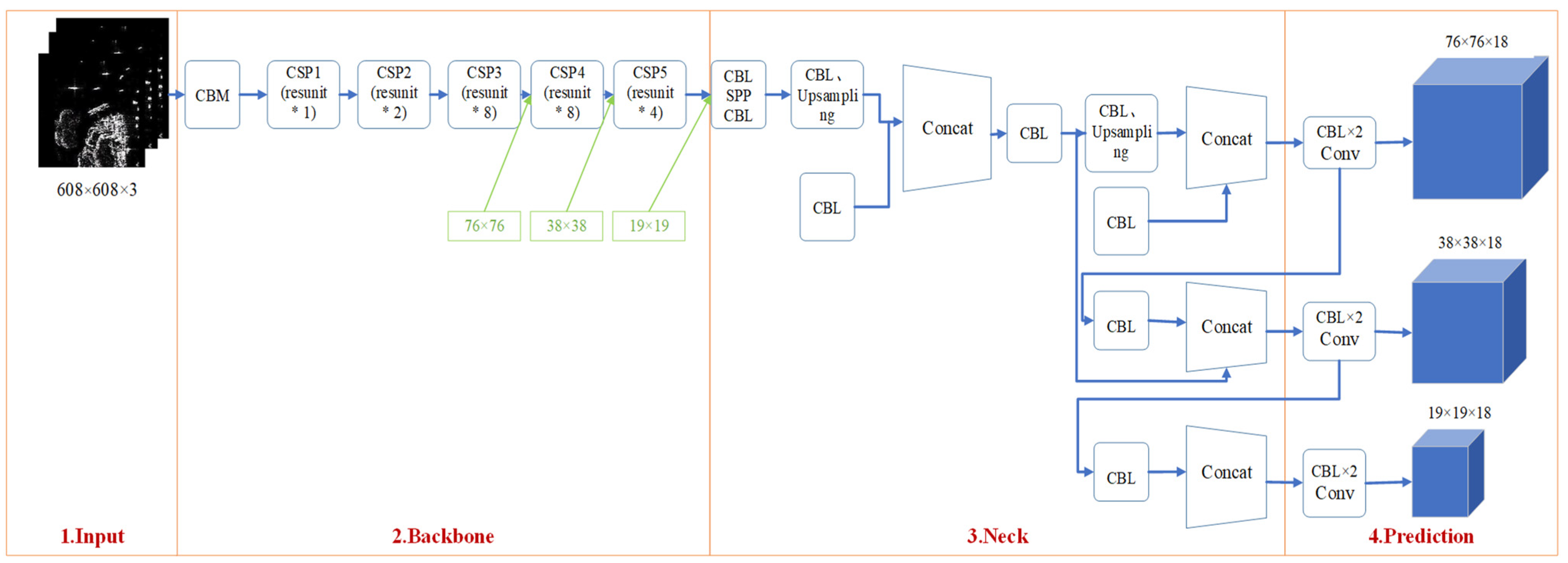
The YOLOv4 detector, shown in Figure 1, utilizes CNN and comprises four components. In object detection algorithms, the “backbone” network could extract the basic features of input images. Cross Stage Partial (CSP) Darknet53 serves this role as the “backbone” network for YOLOv4. The “Neck” module is the third part of top-down and bottom-up propagation with semantic information features through the spatial pyramid pooling (SPP) module. Following the SPP module, the top-down feature pyramid network (FPN) and bottom-up feature pyramid network (PANet) modules are coupled. The detecting head of YOLOv3 is still used in the prediction section. To calculate the distance between the prediction box and the ground truth, the Complete Intersection over Union (CIOU) loss function is employed. To estimate the position of the target frame, the Distance Intersection over Union (DIOU) Non-Maximum Suppression (NMS) approach is adopted.
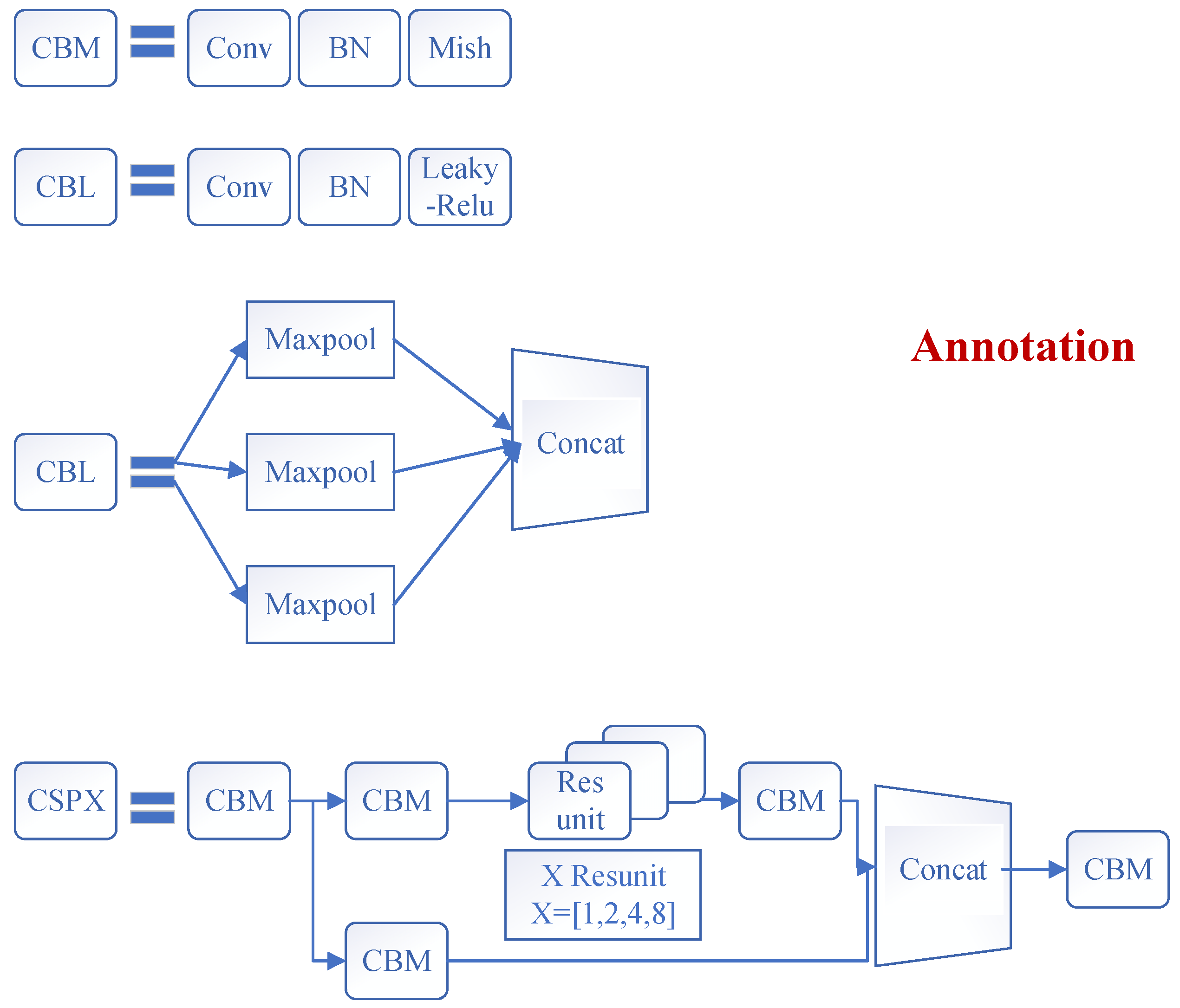
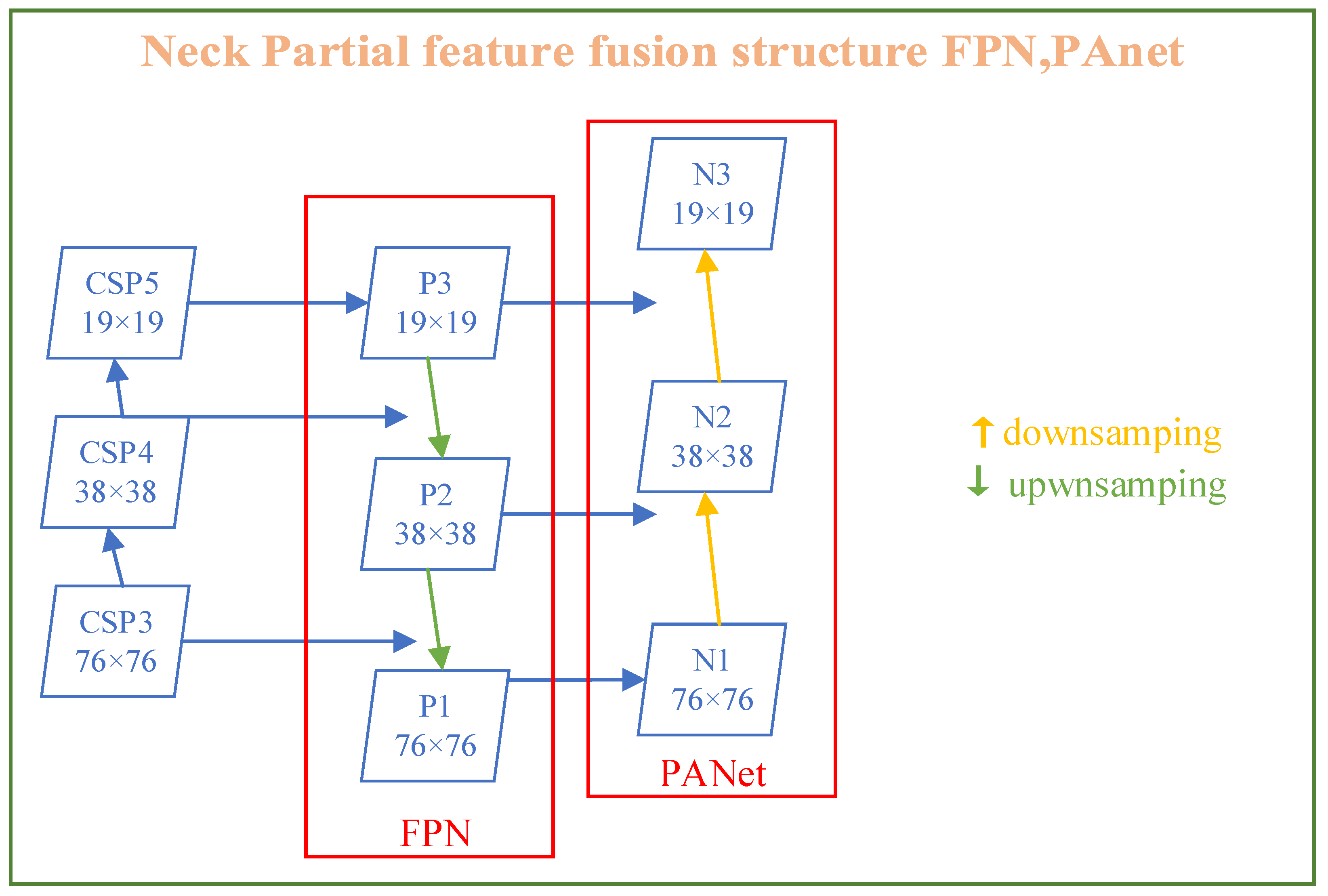
Figure 2 shows the specific modules in the YOLOv4 structure diagram. * represents the multiplication sign. CBM: This component includes operations of convolution (conv), batch normalization (BN), and mish activation function; CBL: This component includes operations of conv, BN, and Leaky_ relu activation function; Resunit: This module is similar to the residual unit used in the Resnet model to help build deeper networks; CSPX: These are a CBM and X Resunits in series; SPP: This is a multiscale fusion module through 1 × 1, 5 × 5, 9 × 9, and 13 × 13 maximum pooling methods. Figure 3 reprents 3D process of feature extraction operation by FPN and PANet.
2.3. Attention Mechanism
The neural network may concentrate on only a portion of its input due to the development of an attention mechanism, which also contributes to the neural network’s high interpretability. As a result, the best-performing models employ an attention mechanism to connect input and output. Vaswani et al. [7] developed the transformer, a new, simple model that depends on the attention mechanism used in machine translation jobs and is free of recurrence and convolutions. This new design takes less time to train. Then, Carion et al. [40] proposed the Detection Transformer (DETR) model, which features a transformer architecture and a global loss-based set that requires predictions. DETR is a based set that constructs a top convolutional backbone using a Transformer model. A standard CNN backbone is capable of learning 2D representations of input pictures. After flattening the transformer encoder, the model adds position encoding. In terms of runtime and accuracy, DETR is comparable to the Faster RCNN baseline for the COCO dataset. The COCO dataset is a collection of demanding, high-quality computer vision datasets that make use of cutting-edge neural networks. The entire dataset’s information is stored in its five components, which are further subdivided into subsections. This highlights the effectiveness of the transformer strategy for CV and machine translation difficulties. Srinivas et al. [41] developed the BoTNet, a backbone architecture, by substituting global self-attention, the main operating unit in the transformer model, for ResNet’s last three bottleneck blocks. A “botnet” is a collection of malware-infected machines supervised by a “bot herder”. In contrast to BoTNet, blocks are added to a ResNet backbone as new blocks rather than replacing existing convolutional blocks. This architecture can perform CV tasks, such as instance segmentation, object detection, and image categorization. As a result, activities involving target recognition in SAR images may also be accomplished using this attention strategy.
3. Materials and Methods
By mimicking the biological visual selection mechanism, the proposed model (Auto-T-YOLO) becomes increasingly similar to the processing of the human visual system, enhancing detection accuracy. During the preattention stage, Auto-T-YOLO automatically identifies the image based on the size of the ship in the image. This stage separates the images into two types: those with large objects and those with only small objects. Moreover, it is analogous to the human preattention visual attention selection mechanism, as it selects simulations based on the size of the targets. The YOLOv4 framework was selected as the core network structure in the attention stage because YOLOv4, a one-stage target detector, can ideally balance speed and accuracy and satisfy the goal of real-time and accurate detection of ship targets. Following that, the notion of global feature precedence in visual perception [10] is incorporated into the proposed model design.
The priority of global features stated by Navon et al. [10] highlights that global aspects are more effective than local features in terms of cognition. Perceptual processes are organized because they progress from global structuring to increasingly fine-grained analysis. After identifying and classifying the target size of remote sensing images through the preattention stage, the YOLOv4 framework processes the semantic aspects of the images sequentially from global to local following the notion of global features preceding local features for large-size target images. In the feature fusion stage, the MHSA module represents a 3 × 3 convolution block for global feature reasoning. This operation analyses and aggregates the global information contained in the feature map that was gathered earlier in the process. The convolution block is connected after the MHSA module to complete the interactive fusion of features from global to local. For images containing only small targets, the YOLOv4 architecture continues to employ the original framework for feature extraction and fusion.
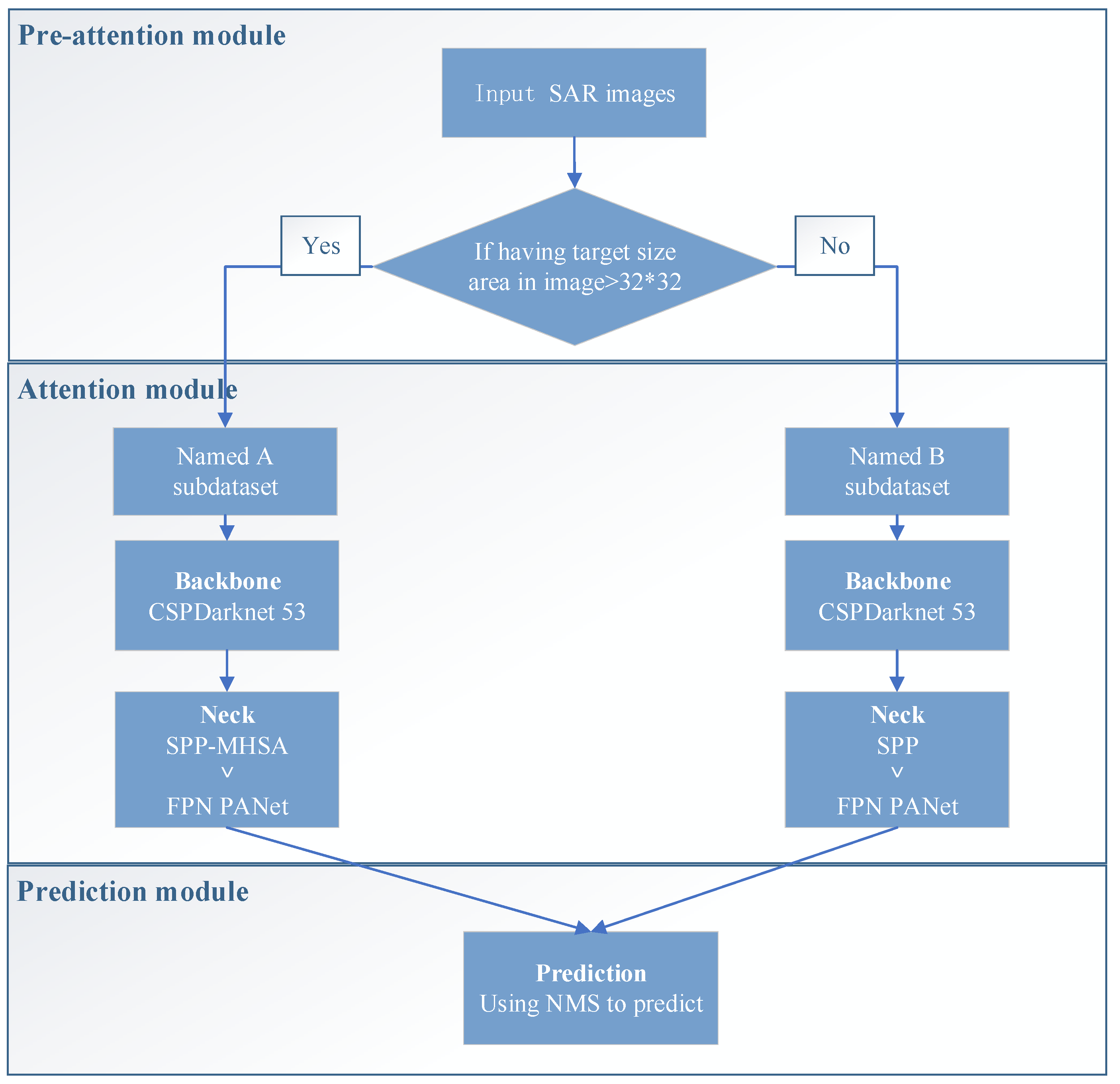
Finally, the two types of images are sent into the network for detection. Figure 4 shows the flow chart of Auto-T-YOLO. * represents the multiplication sign.
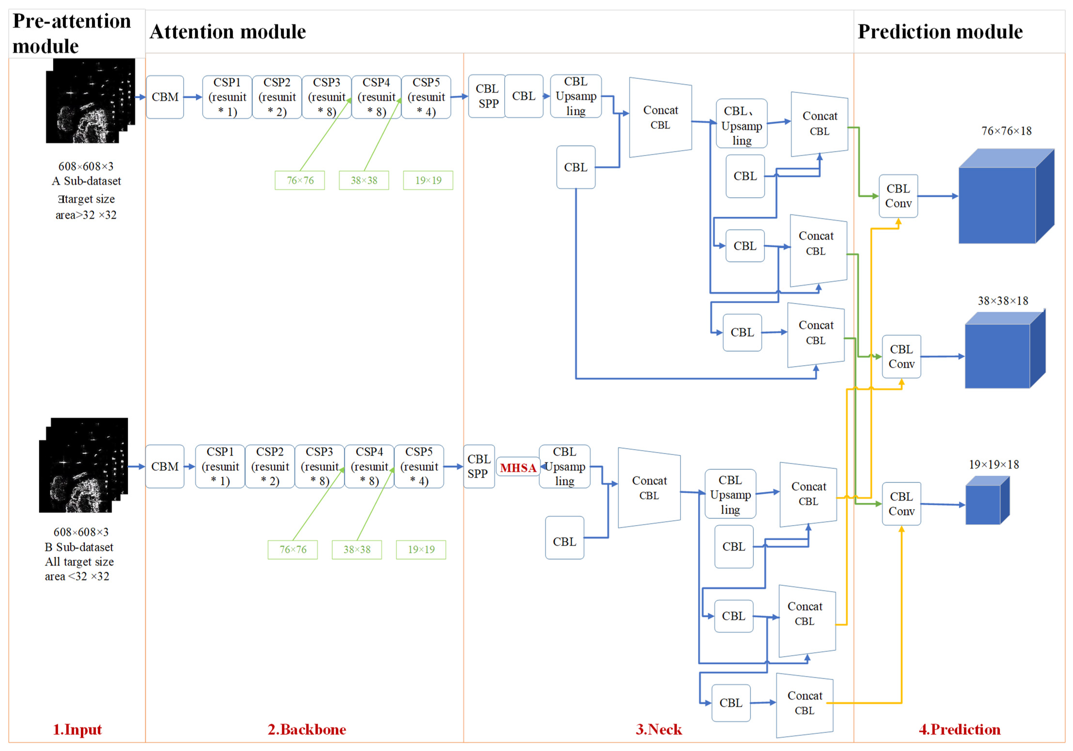
As shown in Figure 4, CSPDarknet53 is used for image feature extraction in the YOLOv4 model. For the A subdataset, the MHSA module was proposed to replace the 3 × 3 convolution block with after SPP module. The image obtained through the MHSA module is transferred to FPN and PANet to accomplish the fusion of global and local features. For the B subdataset, our model uses SPP, FPN, and PANet to fuse context-sensitive features in the Neck module. CNN has a limited receptive field because of the convolutional kernel size restriction. This feature allows the model to be more selective in assessing small targets. The feature maps produced from the A and B subdatasets by the aforementioned methods are detected by YOLOv3′s head.
Figure 5 shows the structure of Auto-T-YOLO through the above flow chart presentation. This model aims to perceive global to local features to better integrate image information and improve target detection. In the third section, the basic operating principles of the algorithm are explained.
The network structure of the model, as illustrated in Figure 5, is separated into three parts: preattention, attention, and prediction module. * represents the multiplication sign. As stated in the introduction, the dataset is divided into A and B based on the target size in the pre-attention module. Following the preattention module, extracting and integrating each image’s characteristics in the SSDD differs in the attention module, and the red font indicates where improvements were achieved. The two subdatasets share a prediction module; the green connecting line represents features taken from the A subdataset for detection, and the yellow arrow represents the B subdataset.
3.1. Preattention Module
According to signal processing, visual attention includes two stages: the preattention stage and the attention stage [42,43]. The preattention stage selects stimuli based on single object attributes, such as color and size, before moving on to the next processing step. In this stage, this study focuses on certain objects and background features. In the attention stage, the features collected from the objects attract human attention. Meanwhile, feature-based attention (FBA) enhances the representation of image attributes across the visual field, which is particularly useful when searching for a specific stimulus feature. In the attention stage, this study can focus on this target first if we can identify key semantic information in the target during the preattention stage. Preattention examines the characteristics since it bases its function on a single feature [8]. Meanwhile, the fusion feature is an operation in the attention stage. The combination of the two stages forms the process of visual attention.
Regarding the sizes of large, medium, and small targets, as shown in Table 1, this study uses the target size definitions in the COCO dataset as a reference. However, considering that the targets in the remote sensing dataset are relatively small compared to the conventional dataset, targets larger than the medium size (area >32 × 32) defined in the COCO dataset are collectively referred to as large-size targets in this study. In addition, the rationality of this setting is justified in the experimental section. This study first classifies the images according to target size. One is an image containing only small-size targets, and the other is an image with large-size targets. Because the visual attention mechanism is simulated in this target detection model, a preattention module is proposed. In the preattention phase, images are classified by target size to better integrate the semantic features of the targets from global to local in the attention phase. The purpose of this operation is based on Navon’s principle of prioritization of global features in visual perception.
The Navon task is a well-known letter identification exercise in which participants are presented with enormous letters made up of a number of much smaller letters as stimuli and are instructed to respond to one type of letter while ignoring the other. Additionally, it monitors global and local processes separately. In Navon’s proposed precedence of global features in visual perception, the visual perception system first deals with the global features and then processes the local features. In the compound stimulus, Navon proposes that the nature of the large images is defined as the global features, and the nature of the small images is defined as the local features, which is equivalent to calling the global features large-scale characteristics and the local features small-scale characteristics. Similarly, the large object in each image is considered a large-scale feature in the task of target detection, and the small-size object is considered a small-scale feature [10].
Previous models used CNNs. However, the size of the convolution kernel limits the receptive field of CNNs. Thus, its modeling range can only be within the receptive field of a convolution kernel. MHSA is a module of the attention mechanism where a separate attention output is combined with a linear transformation to produce a predictive dimension. Meanwhile, the transformer’s MHSA mechanism models global information [7]. Its perception range of self-attention is the entire image. In images with large-size targets, because it is easy for the CNN to fall into the calculation features of the local optimal solution, it usually ignores the surrounding associated features of the large-size targets resulting in insufficient detection accuracy. Therefore, this study introduces the MHSA mechanism into the model and merges the features from global to local in the attention stage. For images that only contain small-size targets, because of the transformer’s superiority in global feature perception, it is easy to ignore the local features of small-size targets. Therefore, small-size targets still use deep CNNs to detect targets.
In the preattention stage, the operation of this module is expressed as follows:
3.2. Attention Module
3.2.1. Backbone: Feature Extraction Network (CSPDarknet53)
Regardless of the subdataset in Figure 5, the YOLOv4 model’s backbone module is still used to extract image features. CSPDarknet53 can extract important semantic features from the YOLOv4 model. As a result, it is employed as a backbone network. As shown in Figure 5, CSPDarknet53 is a CNN that acts as the foundation for object detection by employing DarkNet-53. The feature map on the base layer of a CSPNet network is divided into two parts that are linked together using a CSP-stage hierarchy. The complexity of network optimization can be considerably decreased while keeping accuracy with this network by identifying problems with redundant gradient information. It is compatible with a variety of networks, such as DenseNet, ResNeXt, and ResNet.
In CSPDarknet53, there are five residual blocks that are labeled CSP 1-5. Each residual block (Resunits) has several residual units. Resunit employs the 3×3 convolution operation. This convolution operation includes two steps. The second convolution operation (3 × 3 conv and 1 × 1 conv) is then conducted on each residual block. The overall output is the outcome of these two methods. Figure 6 depicts the particular operational technique. As a result, each residual block can resolve the vanishing gradient problem.
Therefore, the backbone network could extract image features. In our model, the two subdatasets automatically classified after the preattention stage still use CSPDarknet53 to extract target features. CSPDarknet53 enters the feature fusion stage after performing feature extraction since it has a large receptive field and a minimal number of parameters.
Figure 6 contains 29 convolutional layers of 3 × 3 and 5 residual blocks. * represents the multiplication sign. The residual units in each block are 1, 2, 8, 8, and 4. The resolution of the input image of 618 × 618 is set; thus, the output resolution of the third residual block is 76 × 76. The fourth output resolution is 38 × 38, and the fifth output resolution is 19 × 19.
3.2.2. Neck: SPP-MHSA, FPN, and PANet
The extraction of fusion features for target identification is often improved by adding layers between the backbone network and the output layer. YOLOv4′s Neck module includes FPN, PANet, and SPP. The pooling layer, known as SPP, frees the network from the fixed-size constraint, resulting in the CNN no longer having a fixed-size input. The study, in particular, constructs an SPP layer above the final convolution layer. A top-down architecture with horizontal linkages is developed to generate a high-level map of semantic features on a global scale. The FPN design significantly outperforms other generic feature extractors in various applications. Further, PANet is quick, easy, and very efficient. It comprises components that improve information transmission across pipelines. It combines characteristics from all levels and even reduces the distance between the bottom and top layers. Moreover, each level’s elements are enhanced by utilizing augmented routes. This study introduces the transformer’s MHSA module for obtaining important and prominent features from diverse places in images following the SPP module and replacing the convolution block. Figure 7 shows the precise operational procedure. From global to local elements in the images, modeling may be performed. This procedure can be more simply integrated than before and extracts useful semantic and geographical information.
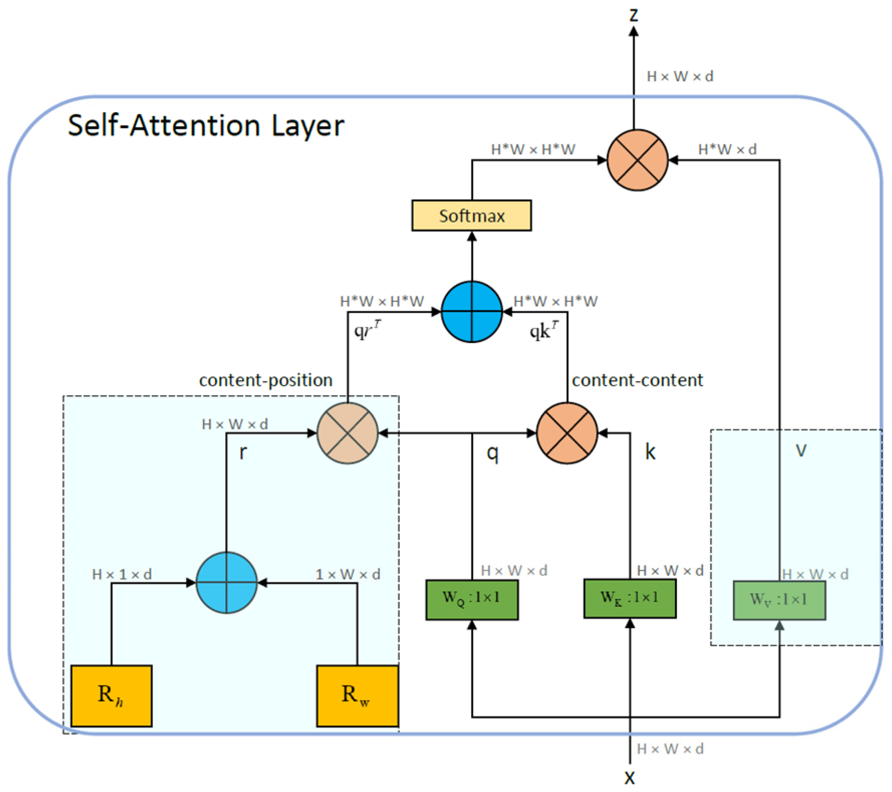
Transformer’s MHSA. The transformer model mainly introduces MHSA, composed of multiple self-attention mechanisms. For this self-attention model, the calculation process could be summarized as a function:
The input is x, representing a matrix in image processing, and the elements in the matrix are called tokens. Linear operations are performed on x to obtain Q, K, V, where Q, K are calculated for similarity and obtain the correlation between each element in Q and K. According to this correlation, the corresponding elements in K are used to construct the output. Similar to the parallel branch in CNN, self-attention can also be designed as a parallel structure called multihead self-attention (MHSA). In Auto-T-YOLO, this study used four heads:
The specific self-attention structure diagram is shown below.
Relative Position Encodings: To perceive the position when performing attention operations, relative position coding is used in the transformer architecture [10]. However, recently, relative-distance-aware position encodings have been found. Relative Position Encodings are a sort of position embedding for Transformer-based models that aim to take advantage of pairwise, relative positional information. The model receives relative positioning information at two levels: values and keys.
The coding approach proposed by Shaw et al. [44] is more suitable for visual processing tasks [45,46]. This can be attributed to the attention mechanism considering the content information and the relative distance of the features in different positions. Based on these considerations, the perception of information and location can be linked more effectively. In SPP-MHSA, this study uses relative position-coding to perform self-attention operations [44,47].
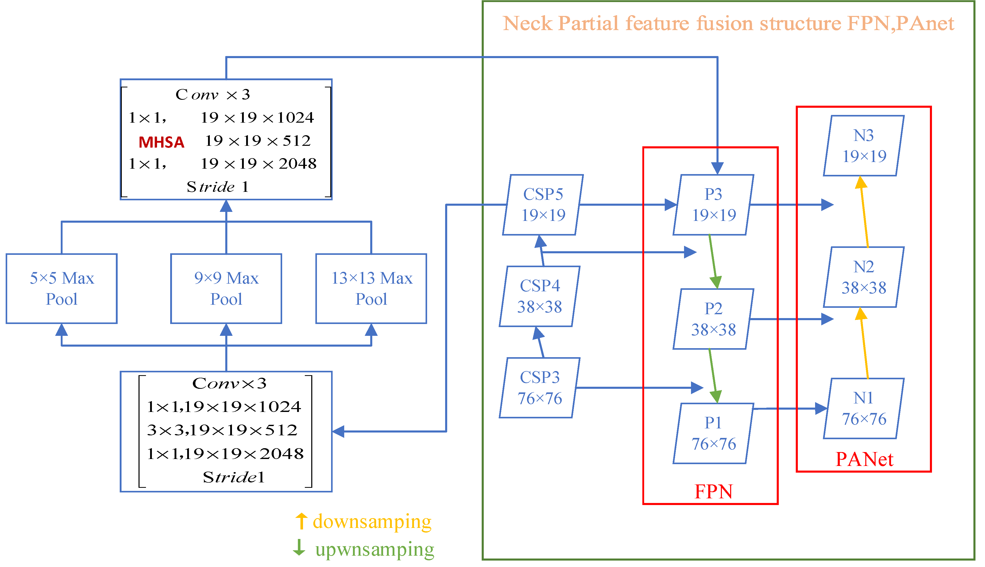
SPP-MHSA. According to the previous analysis, deep CNNs can easily lead to the optimal local solution. It is easy to ignore the salient global features of some targets. The MHSA mechanism aims to model global features. Based on the precedence of global features in visual perception, the fusion order of semantic features for each target is from global to local. Therefore, to detect images with large targets, this study proposes replacing the convolutional block in the feature fusion stage and at various positions in images with the MHSA module. After replacing the convolution block with the SPP module, this study renames the transformer’s MHSA as the SPP-MHSA module.
Figure 8 depicts the particular operation. The model’s first spatial (3 × 3) convolutions are replaced by an MHSA layer that employs global self-attention of a 2D feature map. This was included at the beginning, as shown in Figure 8. The beginning of FPN coincides with the end of CSPDarknet53 because every residual block typically exhibits its strongest characteristics at its deepest layer, and the strongest feature retrieved is in the output of the deepest block at the end of the network. CSPDarknet-53, the YOLOv4 backbone, is responsible for extracting numerous characteristics from images via 5 Resblocks (C1–C5). The network has 53 convolution layers ranging in size from 1 × 1 to 3 × 3. The feature map generated from the MHSA operation can be considered by each succeeding layer and multiscale feature fusion and extraction based on FPN and PANet network design. This is also analogous to transferring the global features perceived by the MHSA layer to the succeeding deep CNN, thus modeling semantic information from global to local using the MHSA layer first, then the convolutional layer. After replacing the block with the MHSA layer, no further operations are necessary because the stride of the convolution block is 1. This enhancement (SPP-MHSA) permits global information to be acquired from feature maps with varying receptive field sizes, and a multiscale fusion of global information can be conducted in subsequent operations. This enhances the model’s detection accuracy for large-size targets.
As shown in Figure 7, the present study used four heads. * represents the multiplication sign. The 3D nature of the feature map passed to the module is determined by the , putting these feature maps as . Pointwise convolution is represented by , ⊕ is the element-wise sum, and ⊗ represent matrix multiplication. When represents height and represents width, and are relative position encodings. Add the and together and output as , representing the position distance coding. Matrix multiplication of obtains content-position (content-position) output , and matrix multiplication of obtains content-content (content-content) output . After , softmax normalization is applied to the obtained matrix, where represent query, key, and position encodings, respectively (this study uses relative distance encodings [38,41,42,43]). After processing, the matrix is , and then this matrix is multiplied by the weight . The final output . In addition to using multiple heads, we introduce a two-dimensional position encoding in the content-position section to accommodate the matrix form in image processing. It differs most from the Transformer mechanism [38,48,49].
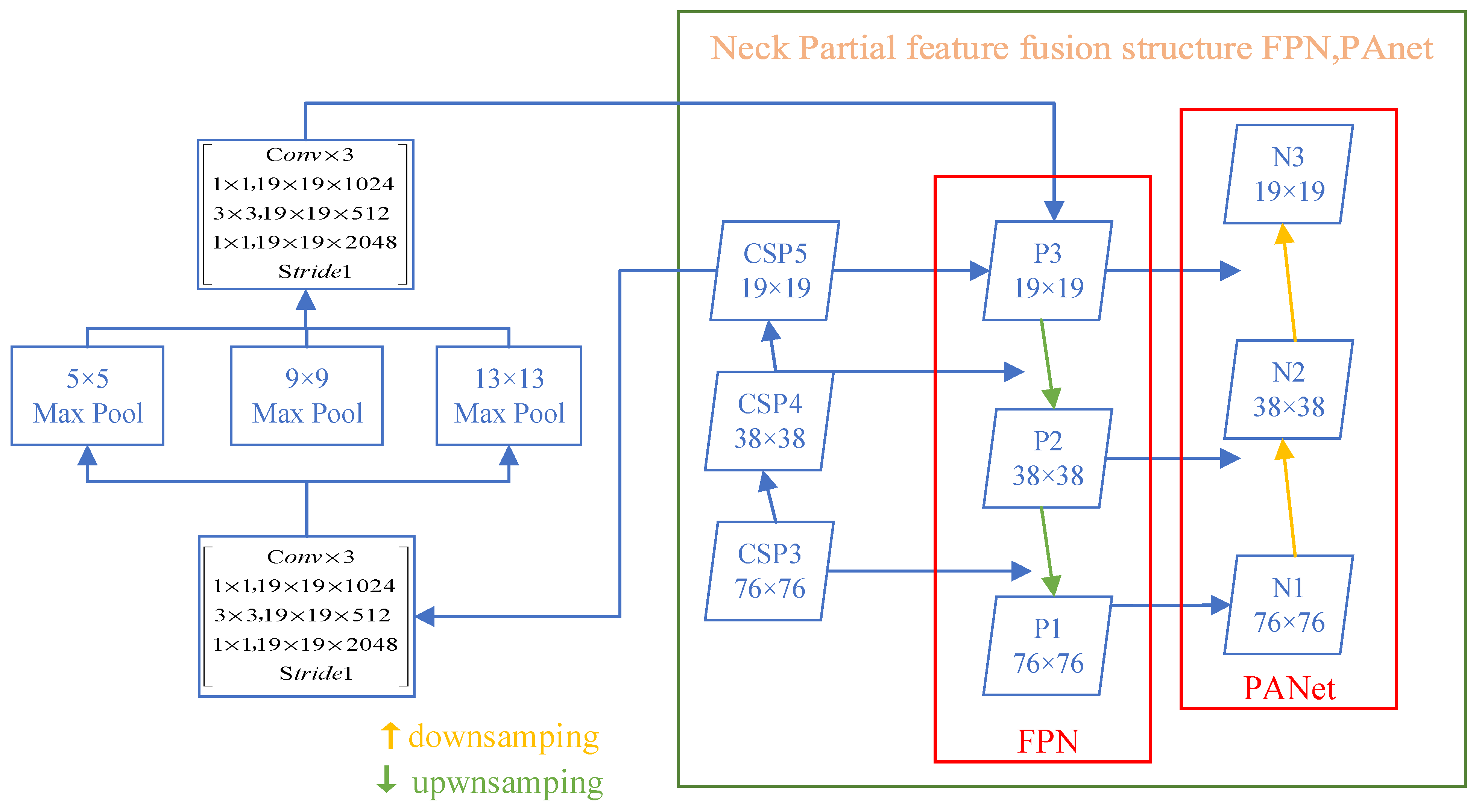
MHSA focuses more on global information. In Figure 9, the important semantic features of small target images are in the surroundings of the targets and are transferred between contexts. Global information can sometimes cause redundancy in the transfer of essential features of small-size targets. Therefore, this study used convolution operations and attention mechanisms to separate the most significant context features instead of using the self-attention mechanism in the attention stage for detecting small-size target images.
In Figure 9, the bold red part is to replace the 3×3 convolution block position with the MHSA layer.
3.3. Prediction Module
3.3.1. CIoU Loss Function
The loss function of object detection usually is constructed from a classifying loss function and a regression loss function for boundary box regression. Because the initial bounding boxes for the truth and bounding boxes for candidates overlap, their intersection ratio is IoU. Scale invariance is a desirable characteristic of IoU. This indicates that the two bounding boxes are considered together with their width, height, and placement. The area of the forms, regardless of their size, is the focus of the normalized IoU measure. The change from norm loss to IoU loss in boundary box loss functions is based on the application of the metric as a loss function. Thus, the IoU’s mathematical formula is given:
This relevant loss function is:
The prediction box is after training. is called a ground truth bounding box, which is also the premarked target ground. If the extracted candidate object is not covering the box delimiting the main claim, LIoU is 1. The Generalized Intersection over Union (GIoU) loss [50] will put a large box outside, which is equivalent to a penalty item. DIoU loss [51] considers the distance between the overlapping area and the center point. If the target frame contains a prediction frame, the distance between them can be calculated directly. However, specific to our prediction task, this study must also consider the geometric factor of the target frame aspect ratio; thus, CIoU has also made improvements to this point, for example, by increasing the compliance limit.
Positive weight parameters are denoted by α. The function measuring the consistency of the aspect ratio is denoted by ν. The width of the target bounding box is . The target bounding box‘s height is .
This study should consider the overlap area, the distance from the center, and the aspect ratio. This study applies the objective box for the regression loss function as the CIoU loss. This loss function speeds up and improves the regression accuracy of prediction boxes.
3.3.2. DIoU-NMS
In order to filter the projected bounding boxes, this study applies nonmaximum suppression operation (NMS). The CV technique known as NMS is used for many tasks. It is a sort of algorithm that chooses one entity from among numerous overlapping instances. A set of criteria is chosen to produce the intended effects. In NMS, which suppresses redundant boxes by taking into consideration both the overlap area and the separation distance between two center points in two bounding boxes, DIoU can be utilized as a criterion. This makes NMS more resistant to occlusion conditions. The typical NMS approach is utilized the most frequently out of all the target detection methods. Our model employs DIoU instead of the computed portion of the IoU and is based on the DIoU/CIoU loss approach. The DIoU loss remains insensitive to the size of the regression problem. If the bounding box does not overlap with the target box, such as GIoU loss, DIoU loss might offer movement directions. It converges significantly more quickly than GIoU loss because DIoU loss may directly decrease the distance between two boxes. As a result, DIoU serves as NMS’s judgmental foundation. DIoU-updated NMS’s formula considers both the area of overlap and the center space distance between the two boxes. can be formally defined as:
If the center lengths of the IoU and the two boxes are also taken into account, the can freely eliminate. means the categorization score, while NMS denotes the NMS threshold. Two boxes, with a central point located apart from each other, can be placed on a large number of objects according to the DIoU-NMS technique. The main difference between DIoU-NMS and NMS is not to delete the two boxes mentioned earlier. At each threshold, the tests in the program [52] show that DIoU-NMS outperforms ordinary NMS. Consequently, the final prediction box in Auto-T-YOLO is screened using the DIoU-NMS approach.
4. Experiments and Results
The inshore and offshore scenarios from two subdatasets of the public SSDD were used in the experiments in this paper. These allow us to validate the efficiency, generalizability, and robustness of Auto-T-YOLO. This part presents the dataset content, the experimental platform, the experimental results, and some analysis.
4.1. SSDD
The SSDD made the first ship-specific dataset in SAR images available to the public. Additionally, labels and bounding boxes are designed following the Pattern Analysis, Statistical Modeling, and Computational Learning Visual Object Classes (POACAL VOL) standard. The information that can be seen in Table 2 reveals that SSDD has a total of 1160 images. Out of these images, a total of 947 were offshore and 213 were inshore images. The majority of the images were taken through sensors. The study used the COCO dataset for the definition of target size and counted the number of images. The number of images whose target size area is >64 × 64 is the least inshore or offshore in Table 2. If the pre-attention stage is divided into A and B subdatasets, the threshold is set to be >64 × 64, and the help for the improvement of model accuracy will be small. SSDD dataset details are in Table 3. Our conjecture has also been verified in Section 4.3.1. In the experimental section of Section 4, the ratio of the training set is 70%. The ratio of the validation set is 20%, and the test set is 10% [31].
4.2. Settings
The Python language used in our experiment was based on the PyTorch framework. PyTorch is a free, open-source machine learning framework built using Python and Torch libraries. It is one of the most recognized research platforms for deep learning. The framework is intended to minimize the length between the research prototype and deployment. This study used Ubuntu 18.04.2 as the operating system with the graphics card of Nvidia RTX 2080Ti. The Turing GPU architecture and the all-new RTX platform power GeForce RTXTM graphics cards. It delivers up to six times the speed of the previous generation of graphics cards and introduces real-time ray tracing and AI in games. Because the weights of YOLOv4 are obtained by training the COCO dataset, in order to obtain the weight values of SSDD, this study trained the SAR image dataset from scratch. The pulse was set to 0.9 and the learning rate to 0.001. The maximum number of iterations was 20,000, and the input image size was 608 × 608.
4.3. Standard of Evaluation
The probability that the classifier categorizes the items correctly is referred to as accuracy. If a ship target is detected, the object will likely be accurately identified as a ship. Two types of accuracy measures were considered to evaluate the prospective performance of Auto-T-YOLO. is the fault detection rate.
is missing the alarm rate.
is the false alarm rate.
, , and are defined by:
means the chance of judging objects. It is the rate that the model predicts correctly in data of true.
Sometimes these two metrics do not change in a synchronized manner. If it is not intuitive to determine which algorithm is superior, the F1 indicator can be used:
In the above formulas, is , and is . is the number of the ground truth. represents a true positive number; represents a true negatives number; is a false positives number; and is a false negatives number. In general, and are detection metrics used by a single image. For the whole dataset, this study needs to introduce one evaluation standard . It represents the accuracy of the whole dataset and the regional curve under accurate recall.
The relationship between the detection time () and frames per second () of a SAR image is:
4.3.1. Target Size Threshold Setting
The study trains Auto-T-YOLO on SSDD (including offshore and inshore scenes). In the preattention module, Auto-T-YOLO divides the entire dataset into two subdatasets, A and B, based on the target size with an explanation of the target size in the COCO dataset. Due to the difference between the object characteristics in remote sensing and the COCO dataset, the classification process cannot fully operate depending on the definition of the target size for the COCO dataset. Therefore, to identify the appropriate target size for the actual case, the experiments were based on the large-size target (64 × 64) and medium-size target (32 × 32) to train the dataset. The training results illustrated in Table 4 indicate that splitting the dataset based on the target size (32 × 32) is more appropriate for remote sensing images and more efficient in detection.
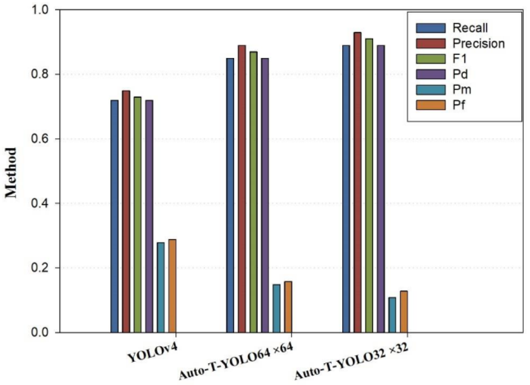
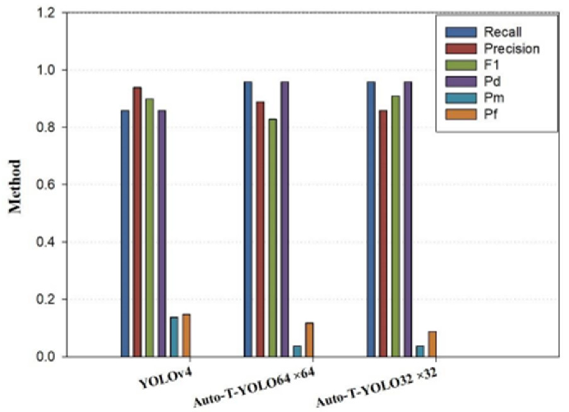
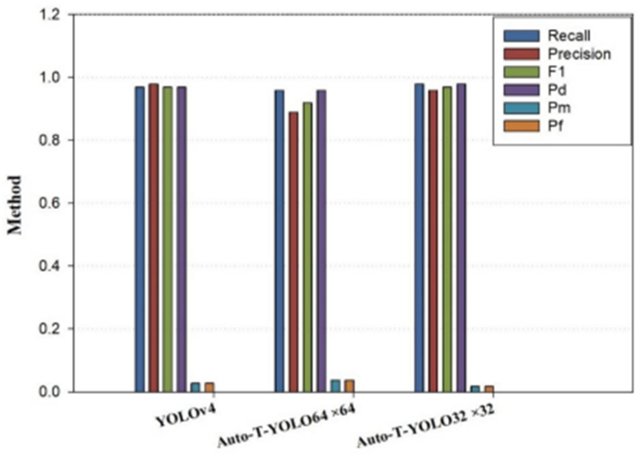
As shown in Table 2, there are a few large-size targets defined by the COCO dataset in the remote sensing images. As shown in Table 4, Table 5 and Table 6, the scores for are all higher than those of . In the inshore scenes, our model has a much higher accuracy than the YOLOv4 model because the ship target size in the inshore scenes is slightly larger. We can also incorporate a transformer mechanism to make it concentrate more on the useful information of the object and extract the essential semantic characteristic information from the overall information because the complicated background has an impact. For offshore scenes, due to the simple background, the characteristics of the area near the ship targets do not contribute much to the target itself. The original YOLOv4 model already has an ideal detection accuracy. The number of images with a target-size area >32 × 32 is three times greater than the number of images with a target-size area > 64 × 64 in Table 2, indicating that the performance of is superior to those of after adding the MHSA module, and the detection accuracy of medium-size targets can be increased once the MHSA module is added. It can be seen that the associated modeling of global semantic information can also supplement the feature information of targets that was lost in the deep CNN. Therefore, Table 4, Table 5 and Table 6 exhibit a combination of experimental findings and target size features from the remote sensing dataset. As shown in Figure 10, Figure 11 and Figure 12, the histograms show the effect of different target size classifications on the experimental results. To employ the SPP-MHSA model for feature fusion extraction, we recommend setting the target area to 32 × 32 in the preattention module stage. If all target sizes in the images are less than 32 × 32, the image features should be processed using the YOLOv4 module.
4.3.2. Impact of the Preattention Module on SSDD including Offshore and Inshore Scenes
Using the logic discussed in the earlier sections, this study divided the datasets into two subdatasets, A and B, based on whether or not the target size of the dataset in the experiments is more than 32 × 32. The model without the preattention module is known as YOLOv4-MHSA. Experiments were run on both datasets to see if there was a preattention module and how it affected the detection accuracy of Auto-T-YOLO.
The detection results of the two accuracy evaluation indicators on YOLOv4, YOLOv4-MHSA, and Auto-T-YOLO on SSDD, including offshore and offshore scenes, are shown in Table 7, Table 8 and Table 9, respectively. On the SSDD, without the preattention module, indicators such as detection accuracy are lower than in the models with preattention modules. On the SSDD dataset, the accuracy of Auto-T-YOLO is 1.4% greater than that of YOLOv4-MHSA. When compared to YOLOv4, Auto-T-YOLO has a 6.3% higher accuracy. This shows the effectiveness of the preattention module. Moreover, it has been demonstrated that incorporating the biological optic nerve into the working principle of CV image processing is the appropriate research direction. It enables the network mode to replicate the human brain for image processing features, enhancing detection accuracy.
Auto-T-YOLO has the best performance, as shown in Table 8, with 98.33% mAP. When combined with the image characteristics of offshore scenes, the accuracy of Auto-T-YOLO is only 0.23% higher than that of YOLOv4-MHSA. We believe this is because images of offshore scenes have a simple background, making the MHSA mechanism, which focuses more on global information and senses the larger field, unable to extract more valid information. The accuracy of the YOLOv4 model and YOLOv4-MHSA models can be improved by adding the preattention stage. This also indicates that automatically classifying the target size can enhance the accuracy value of target detection. The improvement of the proposed model’s accuracy also shows that deep CNN can focus more on effective semantic information for images of small-size targets. The results demonstrate that Auto-T-YOLO is more accurate than the other two models, indicating that the detection method for target size classification is effective.
For the inshore scenes on SSDD, the accuracy and other indicators of Auto-T-YOLO is also higher than those of YOLOv4-MHSA and YOLOv4, as illustrated in Table 8. From our previous analysis of SSDD, it can be seen that there are some complex backgrounds for the inshore scenes. Accordingly, the YOLOv4-MHSA is 10.63% more accurate than the YOLOv4. After incorporating the MHSA mechanism, more information is retrieved from the features of the ship’s target region, compensating for YOLOv4’s lack of global information. After including the automatic target size selection mechanism in our model, various network structures are employed for target images of varying sizes. The advantages of the two network structures are pooled, resulting in more accuracy than a single fixed YOLO-MHSA. Moreover, the accuracy of YOLOv4-MHSA is higher than that of YOLOv4, demonstrating the MHSA module’s superiority for identifying medium- and large-size objects and further validating it for image capture global features. The accuracy of Auto-T-YOLO is higher than that of YOLOv4-MHSA, demonstrating that, compared to the transformer mechanism, the convolutional network has certain advantages in detecting small-size targets. Using the precedence of global features in visual perception to detect medium- and large-size targets and incorporating the MHSA module into the model to fuse feature information from global to local can considerably increase the accuracy of target identification tasks.
4.3.3. Figures of the Results of Some Ablation Experiments
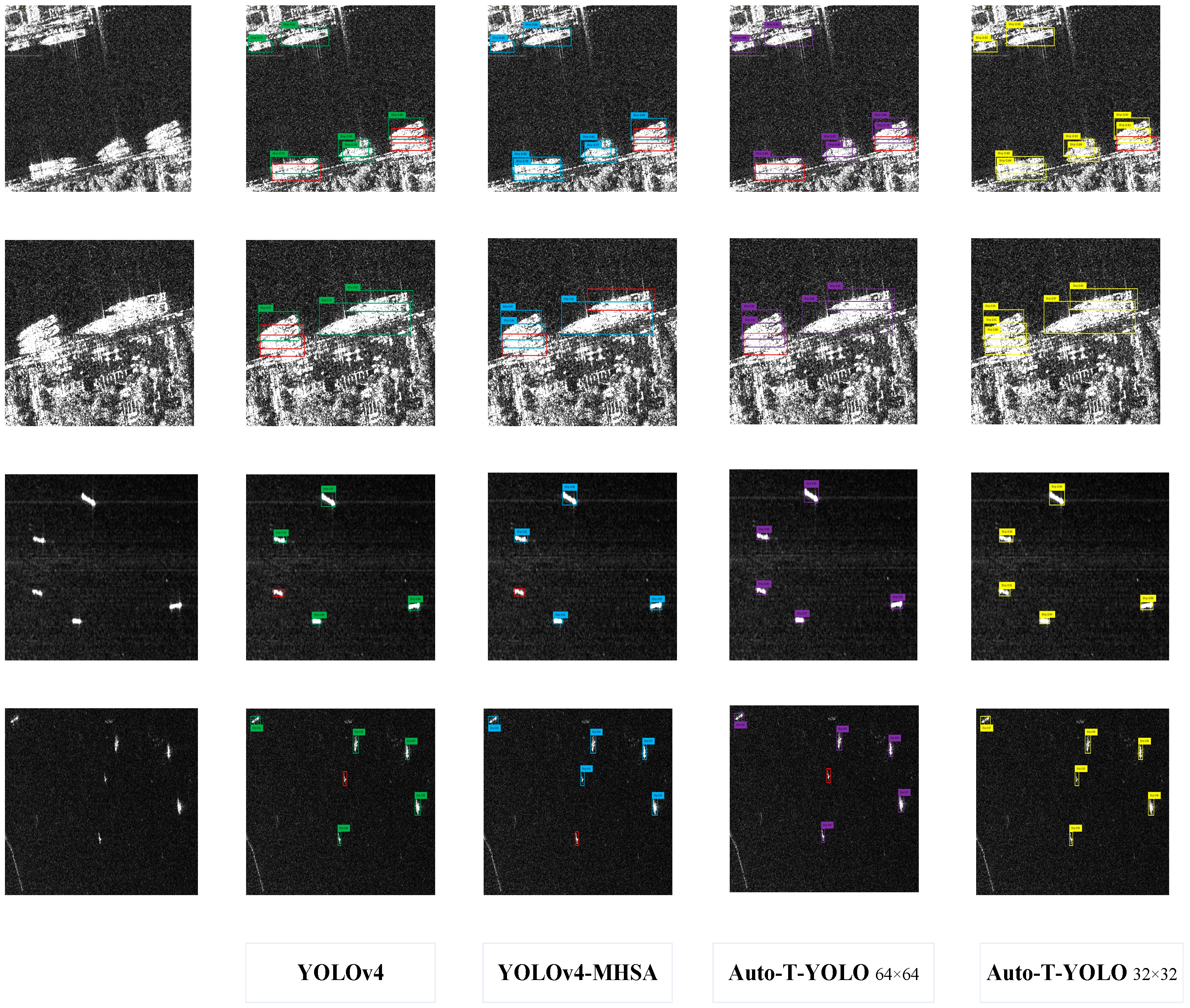
In Figure 13, the first two lines are inshore scenes. The remaining two lines are offshore scenes. The red detection box is the ship target not detected by models. As shown in the figure, the detection accuracy of is higher than that of in rows 1 and 2. The red ground represents the ship target that the model failed to detect. Therefore, it can be seen that the of in the inshore scene is also higher than that of . This demonstrates how we use the MHSA mechanism to extract target semantic information from global to local, allowing critical aspects to be highlighted while reducing the impact of redundant information. In the preattention stage, setting the threshold to Auto—T—YOLO (32 × 32) is also more appropriate for remote sensing image features and considerably enhances accuracy. When comparing the images of YOLO-MHSA and Auto-T-YOLO in rows 1 and 2, it can be seen that for some small-size ship targets that are reasonably close, the MHSA mechanism will incorrectly classify the two ship targets as one because it focuses on global information. Therefore, we can demonstrate the need to include a preattention stage. Following automatic classification, different feature extraction and fusion models can be employed to target features of varying sizes to improve accuracy and efficiency. Although the overall accuracy for the offshore images in rows 3 and 4 is already strong, there are still numerous missed targets in the YOLOv4-MHSA model. This also demonstrates that the MHSA mechanism’s detection accuracy is not optimal for small-size objects. In the next step, this is where we need to work on making improvements. However, based on the visual ship detection findings, it is concluded that Auto-T-YOLO is the best in terms of detection results.
4.4. Comparison with SOTA Models
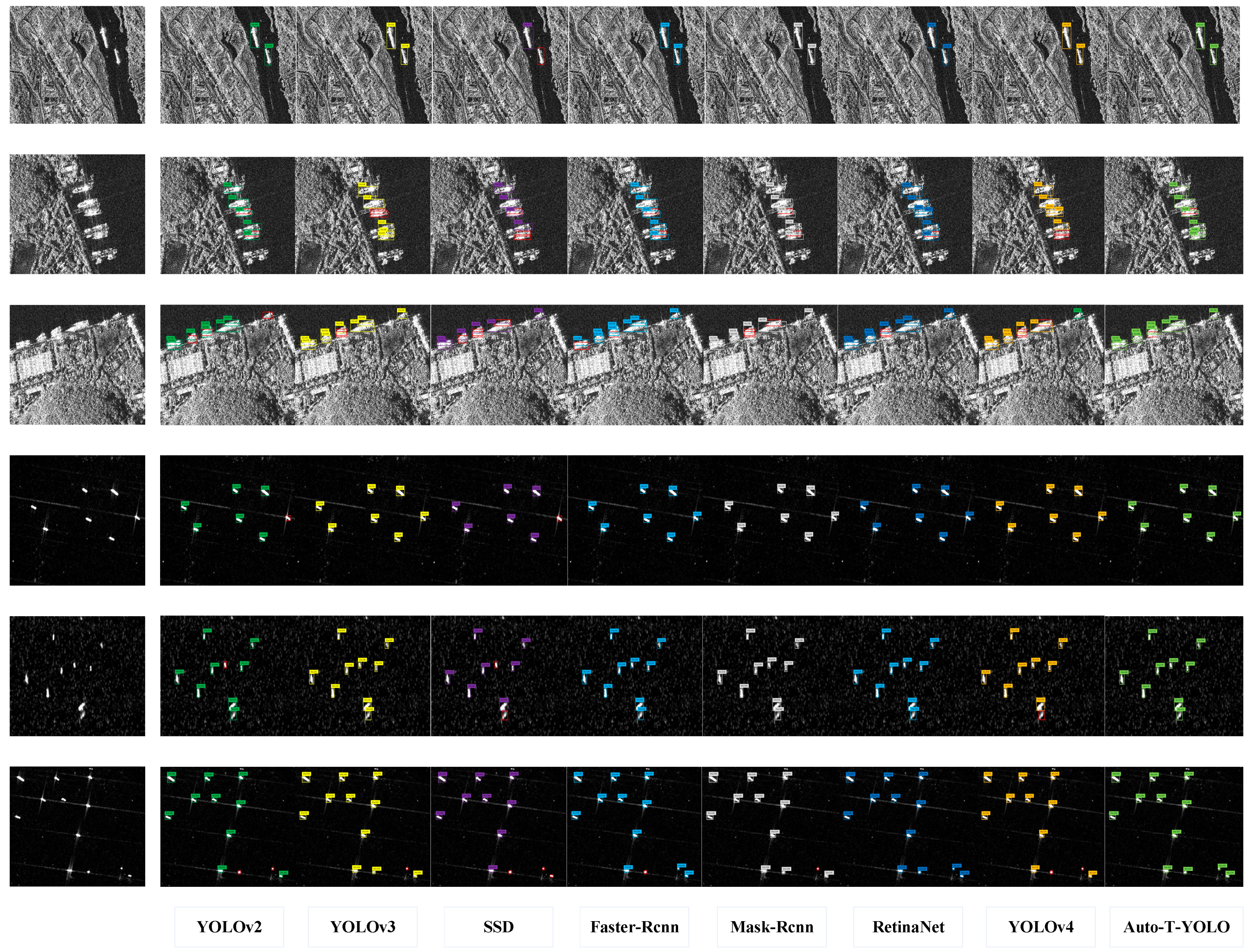
To validate this study’s findings, Auto-T-YOLO was compared to current SOTA models. The field of target detection was introduced to remote sensing imaging. In addition, two accuracy assessment measures were used to assess the effectiveness of the detecting model. Figure 14 depicts the visualization results of different detection models on inshore and offshore scenes from the SSDD dataset. The following discussions and conclusions are based on Table 10, Table 11 and Table 12.
In Table 10, the Auto-T-YOLO model has the highest accuracy compared to the other SOTA models. In terms of accuracy, Auto-T-YOLO is 2.1% is better than the Retinanet model, which is the second best. Model detection is also faster than Retinanet. However, the added characteristics and computational complexity of the model cause a drop in speed compared to one-stage detectors (YOLOv2 and YOLOv3). However, the proposed model is more accurate. Compared to two-stage detection systems, Auto-T-YOLO has fewer parameters, reduced computing complexity, and higher accuracy. Although the FPS of our proposed model is not the highest, as shown in Table 10, yet, when compared to the highest FPS of YOLOv2, the model’s detection accuracy improves by 6% without significantly increasing detection time. Based on the above discussions, it can be concluded that improving Auto-T-YOLO results in a notable improvement in accuracy.
As shown in Table 11, while the accuracy of Auto-T-YOLO is 0.07% lower than that of the ARPN model, it is 1.6 times faster in terms of operating speed. In addition to the ARPN model, Auto-T-YOLO outperforms Retinanet by 0.32% and is 1.7 times faster. Speed and accuracy are important indicators for assessing the model’s performance in terms of real-time target detection. There is sufficient evidence that suggests that Auto-T-YOLO optimally balances the relationship between accuracy and speed in real-world application scenarios. The results in Table 12 show that Auto-T-YOLO has the highest accuracy in inshore scenarios. The AP of 91.87% achieves gains of 11.78%, 10.64%, 9.68%, and 7.68% using HR-SDNet, Fater RCNN, RetinaNet, and ARPN, respectively, with an accuracy rate of more than 80%. On inshore scenarios, our model outperforms the ARPN model. This demonstrates that for complicated backgrounds and large-size targets, the approaches of automatically selecting the suitable structure based on image size and the MHSA mechanism for feature extraction from global to local provide a more successful approach. Therefore, combining the transformer mechanism and the deep CNN is feasible to perform a multiscale fusion of features from the global to the local. Moreover, a model that simulates human visual selective attention mechanisms can be used to improve object detection accuracy. Comparison with detection results of different SOTA algorithms in the SSDD (containing inshore and offshore scenarios) reveals that Auto-T-YOLO has strong generalization capability. Compared to SOTA models, Auto-T-YOLO achieves the appropriate balance of accuracy and speed and the optimal speed and accuracy.
In Figure 14, the first three rows are inshore scenes. Others are offshore scenes. The red detection box represents the ship target not detected by the detection model. These visualization results also corroborate what is shown in the tables above. Compared with the SOTA method, Auto-T-YOLO has the highest accuracy. In inshore scenes, Auto-T-YOLO showed a significantly reduced missed detection rate (1-recall) compared with the values of YOLOV2, YOLOV3, and SSD. The accuracy rate for the offshore scenes was also significantly improved. These visualization results also represent the superiority of the model.
5. Discussion and Conclusions
The current study addresses the issue of edge features for ship objects with large sizes or irregular aspect ratios, which result in poor detection accuracy. Moreover, deep CNN only mechanically learns image features and cannot automatically update the structure with the image features during computation. To solve these issues, the present study introduced an enhanced object detection model that combines the features of the transformer mechanism and CNN. To overcome the problem of the target’s edge features, which are easily ignored, feature fusion is accomplished from global to local for large-size images and medium-size targets. The proposed method, which simulates the human visual attention pattern, chooses distinct structures based on image attributes for target detection. Moreover, the adopted Auto-T-YOLO model autonomously selects different structures to process different image information to improve the model’s detection level. The results showed that once the network structure is incorporated into the preattention and attention stages, the detection accuracy improves, providing some interpretability for the deep CNN’s black-box operation.
Inshore and offshore images for remote sensing have distinct characteristics. Offshore images feature small ship targets against plain backgrounds, and inshore images feature larger ship targets against complex backgrounds. As a result, individually detecting various types of images can show the model’s adaptability and usefulness. In addition, the study used two distinct assessment indexes to validate the detection performance, both of which improved the detection accuracy of the YOLOv4 model. Compared to the SOTA technique, the experimental findings proved the efficacy and superiority of Auto-T-YOLO over existing SOTA ship detectors in terms of target detection.
Although this study’s findings indicated that the proposed model achieves high detection accuracy, there is still potential for improvement. Due to model limitations, it is impossible to change the position of the inspection frame to the ship’s bow clew angle for more accurate detection. Researchers should focus on better integrating the transformer mechanism with the CNN in the future to improve decontamination accuracy and make the network structure consciously detect and process the ship based on its bow clew angle. There is also potential to improve the model’s detection accuracy on inshore images. Meanwhile, the model’s framework will be modified to lower the algorithm’s complexity in the subsequent study.
Author Contributions
Conceptualization, B.S. and X.W.; methodology, B.S. and X.W.; formal analysis, B.S. and F.D.; investigation, B.S., X.W. and A.O.; resources, X.W. and F.D.; data curation, B.S. and A.O.; writing—original draft preparation, B.S. and X.W.; writing—review and editing, B.S., X.W. and A.P.; visualization, B.S. and X.W.; supervision, X.W.; project administration, B.S., X.W. and A.P.; funding acquisition, X.W. All authors have read and agreed to the published version of the manuscript.
Funding
This work was supported by the National Natural Science Foundation of China under Grant 61872231 and Grant 61701297.
Institutional Review Board Statement
Not applicable.
Informed Consent Statement
Not applicable.
Data Availability Statement
Not applicable.
Conflicts of Interest
The authors declare no conflict of interest.
References
- Brusch, S.; Lehner, S.; Fritz, T.; Soccorsi, M.; Soloviev, A.; van Schie, B. Ship surveillance with TerraSAR-X. IEEE Trans. Geosci. Remote Sens. 2010, 49, 1092–1103. [Google Scholar] [CrossRef]
- Crisp, D.J. A ship detection system for RADARSAT-2 dual-pol multi-look imagery implemented in the ADSS. In Proceedings of the 2013 International Conference on Radar, Adelaide, Australia, 9–12 September 2013; pp. 318–323. [Google Scholar]
- Torres, R.; Snoeij, P.; Geudtner, D.; Bibby, D.; Davidson, M.; Attema, E.; Rostan, F. GMES Sentinel-1 mission. Remote Sens. Environ. 2012, 120, 9–24. [Google Scholar] [CrossRef]
- Zhu, C.; Zhou, H.; Wang, R.; Guo, J. A novel hierarchical method of ship detection from spaceborne optical image based on shape and texture features. IEEE Trans. Geosci. Remote Sens. 2010, 48, 3446–3456. [Google Scholar] [CrossRef]
- Liu, Z.; Gu, X.; Chen, J.; Wang, D.; Chen, Y.; Wang, L. Automatic recognition of pavement cracks from combined GPR B-scan and C-scan images using multiscale feature fusion deep neural networks. Autom. Constr. 2023, 146, 104698. [Google Scholar] [CrossRef]
- Wang, S.; Gao, S.; Zhou, L.; Liu, R.; Zhang, H.; Liu, J.; Qian, J. YOLO-SD: Small Ship Detection in SAR Images by Multi-Scale Convolution and Feature Transformer Module. Remote Sens. 2022, 14, 5268. [Google Scholar] [CrossRef]
- Vaswani, A.; Shazeer, N.; Parmar, N.; Uszkoreit, J.; Jones, L.; Gomez, A.N. Attention is all you need. In Proceedings of the Advances in Neural Information Processing Systems, Long Beach, CA, USA, 4–9 December 2017; Volume 30. [Google Scholar]
- Zhang, L.; Lin, W. Selective Visual Attention: Computational Models and Applications; John Wiley & Sons: Hoboken, NJ, USA, 2013. [Google Scholar]
- Liu, Z.; Yeoh, J.K.W.; Gu, X.; Dong, Q.; Chen, Y.; Wu, W.; Wang, D. Automatic pixel-level detection of vertical cracks in asphalt pavement based on GPR investigation and improved mask R-CNN. Autom. Constr. 2023, 146, 104689. [Google Scholar] [CrossRef]
- Navon, D. Forest before trees: The precedence of global features in visual perception. Cognit. Psychol. 1977, 9, 353–383. [Google Scholar] [CrossRef]
- Henschel, M.D.; Rey, M.T.; Campbell, J.W.M.; Petrovic, D. Comparison of probability statistics for automated ship detection in SAR imagery. In Proceedings of the 1998 International Conference on Applications of Photonic Technology III: Closing the Gap between Theory, Development, and Applications, Ottawa, ON, Canada, 4 December 1998; pp. 986–991. [Google Scholar]
- Stagliano, D.; Lupidi, A.; Berizzi, F. Ship detection from SAR images based on CFAR and wavelet transform. In Proceedings of the 2012 Tyrrhenian Workshop on Advances in Radar and Remote Sensing (TyWRRS), Naples, Italy, 12–14 September 2012; pp. 53–58. [Google Scholar]
- Wang, R.; Huang, Y.; Zhang, Y.; Pei, J.; Wu, J.; Yang, J. An inshore ship detection method in SAR images based on contextual fluctuation information. In Proceedings of the 2019 6th Asia-Pacific Conference on Synthetic Aperture Radar (APSAR), Xiamen, China, 26–29 November 2019; p. 19493178. [Google Scholar]
- Ioffe, S.; Szegedy, C. Batch normalization: Accelerating deep network training by reducing internal covariate shift. Int. Conf. Mach. Learn. 2015, 37, 448–456. [Google Scholar]
- Pinheiro, P.O.; Collobert, R. Weakly supervised semantic segmentation with convolutional networks. In CVPR; Citeseer: University Park, PA, USA, 2015; Volume 2, p. 6. [Google Scholar]
- Simonyan, K.; Zisserman, A. Very deep convolutional networks for large-scale image recognition. arXiv 2014, arXiv:1409.1556. [Google Scholar]
- Krizhevsky, A.; Sutskever, I.; Hinton, G.E. ImageNet Classification with Deep Convolutional Neural Networks. Commun. ACM 2017, 60, 84–90. [Google Scholar] [CrossRef] [Green Version]
- Szegedy, C.; Liu, W.; Jia, Y.; Sermanet, P.; Reed, S.; Anguelov, D.; Rabinovich, A. Going deeper with convolutions. In Proceedings of the IEEE Conference on Computer Vision and Pattern Recognition, Boston, MA, USA, 7–12 June 2015; pp. 1–9. [Google Scholar]
- He, K.; Zhang, X.; Ren, S.; Sun, J. Deep residual learning for image recognition. In Proceedings of the IEEE Conference on Computer Vision and Pattern Recognition, Las Vegas, NV, USA, 26 June–1 July 2016; pp. 770–778. [Google Scholar]
- Huang, G.; Liu, Z.; Van Der Maaten, L.; Weinberger, K.Q. Densely connected convolutional networks. In Proceedings of the IEEE Conference on Computer Vision and Pattern Recognition, Honolulu, HI, USA, 21–26 July 2017; pp. 4700–4708. [Google Scholar]
- Tan, M.; Le, Q. Efficient net: Rethinking model scaling for convolutional neural networks. Int. Conf. Mach. Learn. 2019, 97, 6105–6114. [Google Scholar]
- Liu, W.; Anguelov, D.; Erhan, D.; Szegedy, C.; Reed, S.; Fu, C.Y.; Berg, A.C. Ssd: Single shot multibox detector. In Proceedings of the Computer Vision—ECCV 2016, 14th European Conference, Amsterdam, The Netherlands, 11–14 October 2016; Springer: Cham, Switzerland, 2016; pp. 21–37. [Google Scholar]
- Liu, S.; Huang, D. Receptive field block net for accurate and fast object detection. In Proceedings of the European Conference on Computer Vision (ECCV), Munich, Germany, 8–14 September 2018; pp. 385–400. [Google Scholar]
- Bochkovskiy, A.; Wang, C.Y.; Liao, H.Y.M. Yolov4: Optimal speed and accuracy of object detection. arXiv 2020, arXiv:2004.10934. [Google Scholar]
- Redmon, J.; Farhadi, A. YOLO9000: Better, faster, stronger. In Proceedings of the IEEE Conference on Computer Vision and Pattern Recognition, Honolulu, HI, USA, 21–26 July 2017; pp. 7263–7271. [Google Scholar]
- Redmon, J.; Farhadi, A. YOLOv3: An Incremental Improvement. arXiv 2018, arXiv:1804.02767. [Google Scholar]
- Redmon, J.; Divvala, S.; Girshick, R.; Farhadi, A. You only look once: Unified, real-time object detection. In Proceedings of the IEEE Conference on Computer Vision and Pattern Recognition, Las Vegas, NV, USA, 26 June–1 July 2016; pp. 779–788. [Google Scholar]
- Ren, S.; He, K.; Girshick, R.; Sun, J. Faster r-CNN: Towards real-time object detection with region proposal networks. In Proceedings of the Advances in Neural Information Processing Systems, Montreal, QC, Canada, 7–12 December 2015; Volume 28. [Google Scholar]
- Lin, T.Y.; Dollár, P.; Girshick, R.; He, K.; Hariharan, B.; Belongie, S. Feature pyramid networks for object detection. In Proceedings of the IEEE Conference on Computer Vision and Pattern Recognition, Honolulu, HI, USA, 21–26 July 2017; pp. 2117–2125. [Google Scholar]
- Chen, C.; Liu, M.Y.; Tuzel, O.; Xiao, J. R-CNN for small object detection. In Proceedings of the Computer Vision - ACCV 2016—13th Asian Conference on Computer Vision, Taipei, Taiwan, 20–24 November 2016; Springer: Cham, Switzerland, 2017; pp. 214–230. [Google Scholar]
- Li, J.; Qu, C.; Shao, J. Ship detection in SAR images is based on an improved faster R-CNN. In Proceedings of the 2017 SAR in Big Data Era: Models, Methods and Applications (BIGSARDATA), Beijing, China, 13–14 November 2017; pp. 1–6. [Google Scholar]
- Wang, Y.; Wang, C.; Zhang, H.; Zhang, C.; Fu, Q. Combing Single Shot Multibox Detector with transfer learning for ship detection using Chinese Gaofen-3 images. In Proceedings of the 2017 Progress in Electromagnetics Research Symposium-Fall (PIERS-FALL), Singapore, 19–22 November 2017; pp. 712–716. [Google Scholar]
- Lin, Z.; Ji, K.; Leng, X.; Kuang, G. Squeeze and excitation rank faster R-CNN for ship detection in SAR images. IEEE Geosci. Remote Sens. Lett. 2018, 16, 751–755. [Google Scholar] [CrossRef]
- Mao, Y.; Yang, Y.; Ma, Z.; Li, M.; Su, H.; Zhang, J. Efficient, low-cost ship detection for SAR imagery based on simplified U-net. IEEE Access. 2020, 8, 69742–69753. [Google Scholar] [CrossRef]
- Zhang, T.; Zhang, X.; Shi, J.; Wei, S. HyperLi-Net: A hyper-light deep learning network for high-accurate and high-speed ship detection from synthetic aperture radar imagery. ISPRS J. Photogramm. Remote Sens. 2020, 167, 123–153. [Google Scholar] [CrossRef]
- Gong, H.; Mu, T.; Li, Q.; Dai, H.; Li, C.; He, Z.; Wang, B. Swin-Transformer-Enabled YOLOv5 with Attention Mechanism for Small Object Detection on Satellite Images. Remote Sens. 2022, 14, 2861. [Google Scholar] [CrossRef]
- Wang, D.; Liu, Z.; Gu, X.; Wu, W.; Chen, Y.; Wang, L. Automatic detection of pothole distress in asphalt pavement using improved convolutional neural networks. Remote Sens. 2022, 14, 3892. [Google Scholar] [CrossRef]
- Gallo, I.; Rehman, A.U.; Dehkordi, R.H.; Landro, N.; La Grassa, R.; Boschetti, M. Deep Object Detection of Crop Weeds: Performance of YOLOv7 on a Real Case Dataset from UAV Images. Remote Sens. 2023, 15, 539. [Google Scholar] [CrossRef]
- Huang, Z.; Li, Y.; Zhao, T.; Ying, P.; Fan, Y.; Li, J. Infusion port level detection for intravenous infusion based on Yolo v3 neural network. Math. Biosci. Eng. 2021, 18, 3491–3501. [Google Scholar] [CrossRef]
- Carion, N.; Massa, F.; Synnaeve, G.; Usunier, N.; Kirillov, A.; Zagoruyko, S. End-to-end object detection with transformers. In Proceedings of the Computer Vision—ECCV 2020: 16th European Conference, Glasgow, UK, 23–28 August 2020; Springer: Cham, Switzerland, 2020; pp. 213–229. [Google Scholar]
- Srinivas, A.; Lin, T.Y.; Parmar, N.; Shlens, J.; Abbeel, P.; Vaswani, A. Bottleneck transformers for visual recognition. In Proceedings of the IEEE/CVF Conference on Computer Vision and Pattern Recognition, Nashville, TN, USA, 20–25 June 2021; pp. 16519–16529. [Google Scholar]
- Bichot, N.P. Neural mechanisms of top-down selection during visual search. In Proceedings of the 23rd Annual International Conference of the IEEE Engineering in Medicine and Biology Society, Istanbul, Turkey, 25–28 October 2001; pp. 780–783. [Google Scholar]
- Peterson, M.S.; Kramer, A.F.; Wang, R.F.; Irwin, D.E.; McCarley, J.S. Visual search has memory. Psychol. Sci. 2001, 12, 287–292. [Google Scholar] [CrossRef] [PubMed]
- Shaw, P.; Uszkoreit, J.; Vaswani, A. Self-attention with relative position representations. arXiv 2018, arXiv:1803.02155. [Google Scholar]
- Bello, I.; Zoph, B.; Vaswani, A.; Shlens, J.; Le, Q.V. Attention augmented convolutional networks. In Proceedings of the IEEE/CVF International Conference on Computer Vision, Seoul, Korea, 27 October–2 November 2019; pp. 3286–3295. [Google Scholar]
- Zhao, H.; Jia, J.; Koltun, V. Exploring self-attention for image recognition. In Proceedings of the IEEE/CVF Conference on Computer Vision and Pattern Recognition, Seattle, WA, USA, 13–19 June 2020; pp. 10076–10085. [Google Scholar]
- Ramachandran, P.; Parmar, N.; Vaswani, A.; Bello, I.; Levskaya, A.; Shlens, J. Stand-alone self-attention in vision models. In Proceedings of the Advances in Neural Information Processing Systems, Vancouver, BC, Canada, 8–14 December 2019; p. 32. [Google Scholar]
- Wang, X.; Girshick, R.; Gupta, A.; He, K. Non-local neural networks. In Proceedings of the IEEE Conference on Computer Vision and Pattern Recognition, Salt Lake City, UT, USA, 18–23 June 2018; pp. 7794–7803. [Google Scholar]
- Xie, C.; Wu, Y.; Maaten, L.V.D.; Yuille, A.L.; He, K. Feature denoising for improving adversarial robustness. In Proceedings of the IEEE/CVF Conference on Computer Vision and Pattern Recognition, Long Beach, CA, USA, 15–20 June 2019; pp. 501–509. [Google Scholar]
- Rezatofighi, H.; Tsoi, N.; Gwak, J.; Sadeghian, A.; Reid, I.; Savarese, S. Generalized intersection over union: A metric and a loss for bounding box regression. In Proceedings of the IEEE/CVF Conference on Computer Vision and Pattern Recognition, Long Beach, CA, USA, 15–20 June 2019; pp. 658–666. [Google Scholar]
- Zheng, Z.; Wang, P.; Liu, W.; Li, J.; Ye, R.; Ren, D. Distance-IoU loss: Faster and better learning for bounding box regression. In Proceedings of the AAAI Conference on Artificial Intelligence, New York, NY, USA, 7–12 February 2020; pp. 12993–13000. [Google Scholar]
- Kang, M.; Ji, K.; Leng, X.; Lin, Z. Contextual region-based convolutional neural network with multilayer fusion for SAR ship detection. Remote Sens. 2017, 9, 860. [Google Scholar] [CrossRef] [Green Version]
Figure 1.
Components of the YOLOv4 model (Including Input, Backbone, Neck, and Head).

Figure 2.
Some specific explanations of the YOLOv4 module.

Figure 3.
3D process of feature extraction operation by FPN and PANet.

Figure 4.
Flow chart of Auto-T-YOLO.

Figure 5.
Auto-T-YOLO structure diagram.

Figure 6.
Structure of CSPDarknet53.

Figure 7.
Multihead Self-Attention (MHSA) layer in Auto-T-YOLO.

Figure 8.
Structure of SPP, FPN, and PANet.

Figure 9.
Architecture of SPP-MHSA, FPN, and PANet.

Figure 10.
Experimental results for models with different target classifications on inshore scenes.

Figure 11.
Experimental results for models with different target classifications on SSDD.

Figure 12.
Experimental results for models with different target classifications on offshore scenes.
Figure 12.
Experimental results for models with different target classifications on offshore scenes.

Figure 13.
Images of ablation experiments result.

Figure 14.
Visual detection results of ships for different models in the SSDD dataset.


Table 1.
Explanation of large, medium, and small target sizes from the COCO dataset.
| small objects | area < 32 × 32 | ||
| medium objects | 32 | × | 32 < area < 64 × 64 |
| large objects | area > 64 × 64 |
Table 2.
There are statistics about the ships’ target-size area in the SSDD dataset. When there is more than one target size area of the ship in the image larger than 64 × 64, this study will count this image as “the number of areas > 64 × 64”. The same as “the number of areas > 32 × 32” is also counted like this. When the target size area of all ships in the image is smaller than 32 × 32, we count this image as “the number of all area < 32 × 32”.
| Name | Number of Areas >64 × 64 | Number of All Area >32 × 32 | Number of All Area <32 × 32 | Total |
|---|---|---|---|---|
| Inshore | 82 | 150 | 64 | 213 |
| Offshore | 206 | 647 | 300 | 947 |
| Total | 288 | 797 | 363 | 1160 |
Table 3.
SSDD dataset details.
| Sensors | Polarization | Scale | Resolution | Position |
|---|---|---|---|---|
| RadarSat-2 TerraSAR-X Sentinel-1 | HH, VV, VH, HV | 1:1 1:2 2:1 | 1 m-15 m | In the sea and offshore |
Table 4.
Experimental results for models with different target classifications on SSDD.
| Method | |||||||
|---|---|---|---|---|---|---|---|
| YOLOv4 | 90.15% | 0.86 | 0.94 | 0.90 | 0.86 | 0.14 | 0.15 |
| 92.48% | 0.92 | 0.89 | 0.90 | 0.92 | 0.08 | 0.07 | |
| 96.3% | 0.96 | 0.86 | 0.91 | 0.96 | 0.04 | 0.09 |
Table 5.
Experimental results for models with different target classifications on offshore scenes.
| Method | |||||||
|---|---|---|---|---|---|---|---|
| YOLOv4 | 97.98% | 0.97 | 0.98 | 0.97 | 0.97 | 0.03 | 0.03 |
| 98.01% | 0.97 | 0.98 | 0.97 | 0.97 | 0.03 | 0.03 | |
| 98.33% | 0.98 | 0.96 | 0.97 | 0.98 | 0.02 | 0.02 |
Table 6.
Experimental results for models with different target classifications on inshore scenes.
| Method | |||||||
|---|---|---|---|---|---|---|---|
| YOLOv4 | 78.73% | 0.72 | 0.75 | 0.73 | 0.72 | 0.28 | 0.29 |
| 85.98% | 0.85 | 0.89 | 0.87 | 0.85 | 0.15 | 0.16 | |
| 91.78% | 0.89 | 0.93 | 0.91 | 0.89 | 0.11 | 0.13 |
Table 7.
Influence of preattention module on SSDD.
| Method | |||||||
|---|---|---|---|---|---|---|---|
| YOLOv4 | 90.15% | 0.86 | 0.94 | 0.90 | 0.86 | 0.14 | 0.15 |
| YOLOv4-MHSA | 94.9% | 0.96 | 0.89 | 0.83 | 0.96 | 0.04 | 0.12 |
| Auto-T-YOLO | 96.3% | 0.96 | 0.86 | 0.91 | 0.96 | 0.04 | 0.09 |
Table 8.
Influence of preattention module on the offshore scenes.
| Method | |||||||
|---|---|---|---|---|---|---|---|
| YOLOv4 | 97.98% | 0.97 | 0.98 | 0.97 | 0.97 | 0.03 | 0.03 |
| YOLOv4-MHSA | 98.1% | 0.96 | 0.89 | 0.92 | 0.96 | 0.04 | 0.04 |
| Auto-T-YOLO | 98.33% | 0.98 | 0.96 | 0.97 | 0.98 | 0.02 | 0.02 |
Table 9.
Influence of preattention module on the inshore scenes.
| Method | |||||||
|---|---|---|---|---|---|---|---|
| YOLOv4 | 78.73% | 0.72 | 0.75 | 0.73 | 0.72 | 0.28 | 0.29 |
| YOLOv4-MHSA | 89.36% | 0.89 | 0.87 | 0.88 | 0.859 | 0.11 | 0.14 |
| Auto-T-YOLO | 91.78% | 0.89 | 0.93 | 0.91 | 0.89 | 0.11 | 0.13 |
Table 10.
Experimental results of SOTA models on SSDD dataset.
| Method | AP | Recall | Precision | F1 | Pd | Pm | Pf | FPS | Param(M) |
|---|---|---|---|---|---|---|---|---|---|
| YOLOv2 | 90.10% | 0.89 | 0.91 | 0.91 | 0.89 | 0.11 | 0.11 | 27 | 217 |
| YOLOv3 | 91.84% | 0.90 | 0.92 | 0.91 | 0.90 | 0.10 | 0.10 | 20.1 | 243.5 |
| SSD | 80.77% | 0.72 | 0.80 | 0.76 | 0.72 | 0.28 | 0.31 | 21.3 | 297.8 |
| Fater R-cnn | 92.94% | 0.71 | 0.92 | 0.76 | 0.71 | 0.29 | 0.38 | 13.3 | 482.4 |
| Mask R-cnn | 92.43% | 0.95 | 0.89 | 0.92 | 0.92 | 0.05 | 0.04 | 12.5 | 503.4 |
| RetinaNet | 94.1% | 0.94 | 0.92 | 0.93 | 0.94 | 0.06 | 0.05 | 12.8 | 442.3 |
| YOLOv4 | 90.15% | 0.86 | 0.94 | 0.90 | 0.86 | 0.14 | 0.15 | 24 | 244.2 |
| Auto-T-YOLO | 96.3% | 0.96 | 0.86 | 0.91 | 0.96 | 0.04 | 0.09 | 20.9 | 247.8 |
Table 11.
Experimental results of SOTA models on offshore scenes.
| Method | AP | Recall | Precision | F1 | Pd | Pm | Pf | FPS | Param(M) |
|---|---|---|---|---|---|---|---|---|---|
| YOLOv3 | 95.39% | 0.99 | 0.95 | 0.97 | 0.99 | 0.01 | 0.01 | 20.1 | 243.5 |
| Fater R-cnn | 97.74% | 0.96 | 0.97 | 0.97 | 0.96 | 0.04 | 0.03 | 13.3 | 482.4 |
| RetinaNet | 97.81% | 0.96 | 0.95 | 0.96 | 0.96 | 0.04 | 0.04 | 12.8 | 442.3 |
| DAPN | 95.93% | 0.99 | 0.96 | 0.98 | 0.99 | 0.01 | 0.01 | 24 | 244.2 |
| HR-SDNet | 92.10 % | 0.94 | 0.95 | 0.94 | 0.94 | 0.06 | 0.06 | 11 | 598.1 |
| ARPN | 98.20 % | 0.96 | 0.97 | 0.96 | 0.96 | 0.04 | 0.04 | 13 | 490.7 |
| Auto-T-YOLO | 98.33% | 0.98 | 0.96 | 0.97 | 0.98 | 0.02 | 0.02 | 20.9 | 247.8 |
Table 12.
Experimental results of SOTA models on inshore scenes.
| Method | AP | Recall | Precision | F1 | Pd | Pm | Pf | FPS | Param(M) |
|---|---|---|---|---|---|---|---|---|---|
| YOLOv3 | 78.50% | 0.71 | 0.73 | 0.72 | 0.71 | 0.29 | 0.30 | 20.1 | 243.5 |
| Fater R-cnn | 81.14% | 0.82 | 0.63 | 0.71 | 0.82 | 0.18 | 0.14 | 13.3 | 482.4 |
| RetinaNet | 82.1% | 0.83 | 0.86 | 0.84 | 0.83 | 0.27 | 0.18 | 12.8 | 442.3 |
| DAPN | 77.20% | 0.72 | 0.69 | 0.70 | 0.72 | 0.28 | 0.27 | 24 | 244.2 |
| HR-SDNet | 80.0% | 0.84 | 0.66 | 0.73 | 0.84 | 0.26 | 0.16 | 11 | 598.1 |
| ARPN | 84.1 % | 0.85 | 0.73 | 0.79 | 0.85 | 0.15 | 0.13 | 13 | 490.7 |
| Auto-T-YOLO | 91.78% | 0.89 | 0.93 | 0.91 | 0.89 | 0.11 | 0.13 | 20.9 | 247.8 |
Disclaimer/Publisher’s Note: The statements, opinions and data contained in all publications are solely those of the individual author(s) and contributor(s) and not of MDPI and/or the editor(s). MDPI and/or the editor(s) disclaim responsibility for any injury to people or property resulting from any ideas, methods, instructions or products referred to in the content. |
© 2023 by the authors. Licensee MDPI, Basel, Switzerland. This article is an open access article distributed under the terms and conditions of the Creative Commons Attribution (CC BY) license (https://creativecommons.org/licenses/by/4.0/).
Share and Cite
MDPI and ACS Style
Sun, B.; Wang, X.; Oad, A.; Pervez, A.; Dong, F. Automatic Ship Object Detection Model Based on YOLOv4 with Transformer Mechanism in Remote Sensing Images. Appl. Sci. 2023, 13, 2488. https://0-doi-org.brum.beds.ac.uk/10.3390/app13042488
AMA Style
Sun B, Wang X, Oad A, Pervez A, Dong F. Automatic Ship Object Detection Model Based on YOLOv4 with Transformer Mechanism in Remote Sensing Images. Applied Sciences. 2023; 13(4):2488. https://0-doi-org.brum.beds.ac.uk/10.3390/app13042488
Chicago/Turabian StyleSun, Bowen, Xiaofeng Wang, Ammar Oad, Amjad Pervez, and Feng Dong. 2023. "Automatic Ship Object Detection Model Based on YOLOv4 with Transformer Mechanism in Remote Sensing Images" Applied Sciences 13, no. 4: 2488. https://0-doi-org.brum.beds.ac.uk/10.3390/app13042488
Note that from the first issue of 2016, this journal uses article numbers instead of page numbers. See further details here.