A Fast Reactive Power Optimization in Distribution Network Based on Large Random Matrix Theory and Data Analysis

Abstract

In this paper, a reactive power optimization method based on historical data is investigated to solve the dynamic reactive power optimization problem in distribution network. In order to reflect the variation of loads, network loads are represented in a form of random matrix. Load similarity (LS) is defined to measure the degree of similarity between the loads in different days and the calculation method of the load similarity of load random matrix (LRM) is presented. By calculating the load similarity between the forecasting random matrix and the random matrix of historical load, the historical reactive power optimization dispatching scheme that most matches the forecasting load can be found for reactive power control usage. The differences of daily load curves between working days and weekends in different seasons are considered in the proposed method. The proposed method is tested on a standard 14 nodes distribution network with three different types of load. The computational result demonstrates that the proposed method for reactive power optimization is fast, feasible and effective in distribution network.

1. Introduction

Voltage control and reactive power optimization (RPO) have been identified as two of the important operation functions in distribution network (DN). The RPO is usually implemented to get the optimal objective by optimally controlling load ratio control transformer, step-voltage regulators, shunt capacitors, shunt reactor, static synchronous compensator (STATCOM), etc. The minimal line loss is often selected as the objectives.

Many researchers, in recent years, have investigated RPO in DN. An optimization approach was proposed in [1] based on recursive mixed-integer programming method. The feature of the proposed algorithm is to treat the capacitor or reactor compensation unit number as a discrete variable. A mixed-integer linear programming method using convexification and linearization was proposed in [2]. Genetic algorithm [3] and the other stochastic search algorithms are global optimization algorithms and suitable for multi-path searching and solving problems with discrete integer constraints. A hybrid optimization algorithm combining with improved GA and continuous linear programming method was proposed in [4], which can obtain the global optimal solution and reduce the computation time.

Based on the one-day-ahead load forecasting, dynamic RPO determines the reactive power control devices action sequence in next day, with the purpose to reduce daily network losses, improve voltage quality and avoid excessive operation [5].

Distributed generation (DG) in DN makes RPO a more complex problem. A trust-region sequential quadratic programming (TRSQP) method is proposed in [6] to solve the RPO problem for distribution networks with DG. With wind power and photovoltaic power introduced into distribution network, the effects of wind generation and photovoltaic generation have been taken into consideration in RPO problems for DN. Uncertain wind power is considered in [7] and photovoltaic power is considered in [8] when optimizing reactive power in DN.

The traditional RPO methods are mathematical model-based methods, and there are two levels. One level is the derivative-based methods using sensibility matrix, Jacobi matrix, Hessian matrix, etc. The second level is the stochastic searching algorithms based methods, such as GA, PSO, etc. Although the traditional methods can formulate accurate mathematical model, many iterations and a lot of time are required in the solution process.

Most previous studies on RPO mainly focused on improving the performance of mathematical programming based and stochastic search algorithm. In addition, the load model is often treated as several simple and fixed typical types. Little effort was focused on utilizing data analysis method on historical data of the RPO.

With a big data method, regularity of RPO can be found to avoid time-consuming iterative calculation and reduce computing time, improving the real-time capability. Some achievement has been made in studies on big data applications in power system currently. In [9], a big data architecture designed for smart grids was proposed based on random matrix theory (RMT). However, the investigation on RPO in DN with big data technology has not yet been carried out. Exploring the regularity in RPO from the historical data of power system, combining with the characteristics of loads can introduce new approach in DN.

Large random matrix theory, with its advantages to deal with mass data, has already been applied to many fields, including signal detection [10], etc. In this paper, the focus of the study is mainly devoted to the sampled covariance matrix’s largest eigen value. Random matrix theory is a big subject with application in many disciplines of science [11], engineering [12], communication [13] and finance [14]. The data of power system shows considerable randomness with the influence of weather, finance, sociocultural, etc. Thus, it is necessary to introduce random matrix theory into power system analysis.

The amount and kind of data in our living world have been exploding. Big data analysis will become a key basis of competition, underpinning new waves of productivity growth and innovation [15]. As the power grid moves to smart grid, the power system has to deal with a large amount of data collected from millions of sensors and integrate series sets of data analytics and applications [16]. Therefore, it is necessary to introduce big data analysis technology into power grid management. With the help of big data technology, we can make corrective, predictive, distributed and adaptive decisions [17].

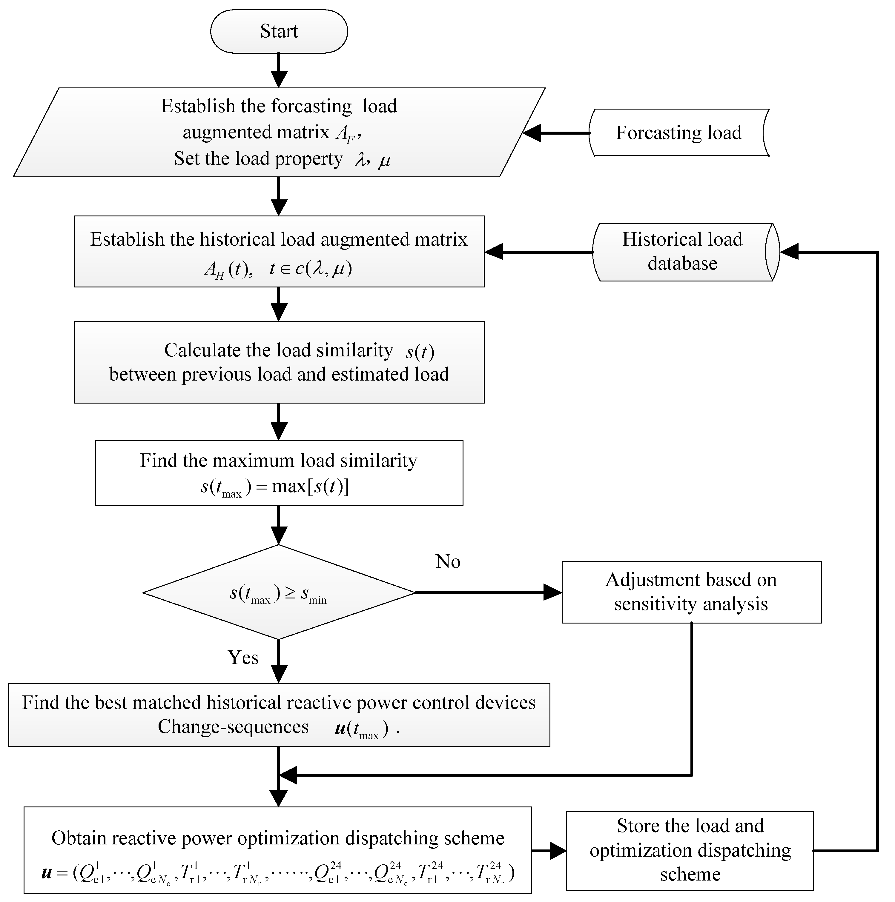
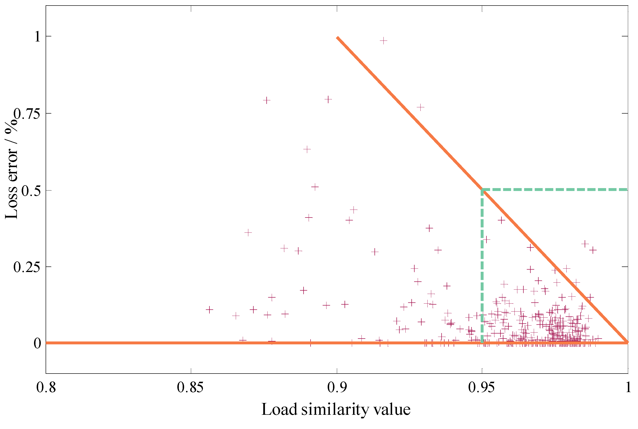
A big data RPO method based on historical data and random matrix (RM) is presented in this paper, whose target is to solve the day-ahead RPO (DPRO) problem by combining with historical load and dispatching scheme of reactive power control devices. Network loads are expressed in a form of RM in this paper. Load similarity (LS) is defined to measure the degree of similarity between the loads in different days. By computing the load similarity between the forecasting load random matrix and the historical load random matrix, the reactive power control approach for one-day-ahead can refer to the historical dispatching scheme of RPO.

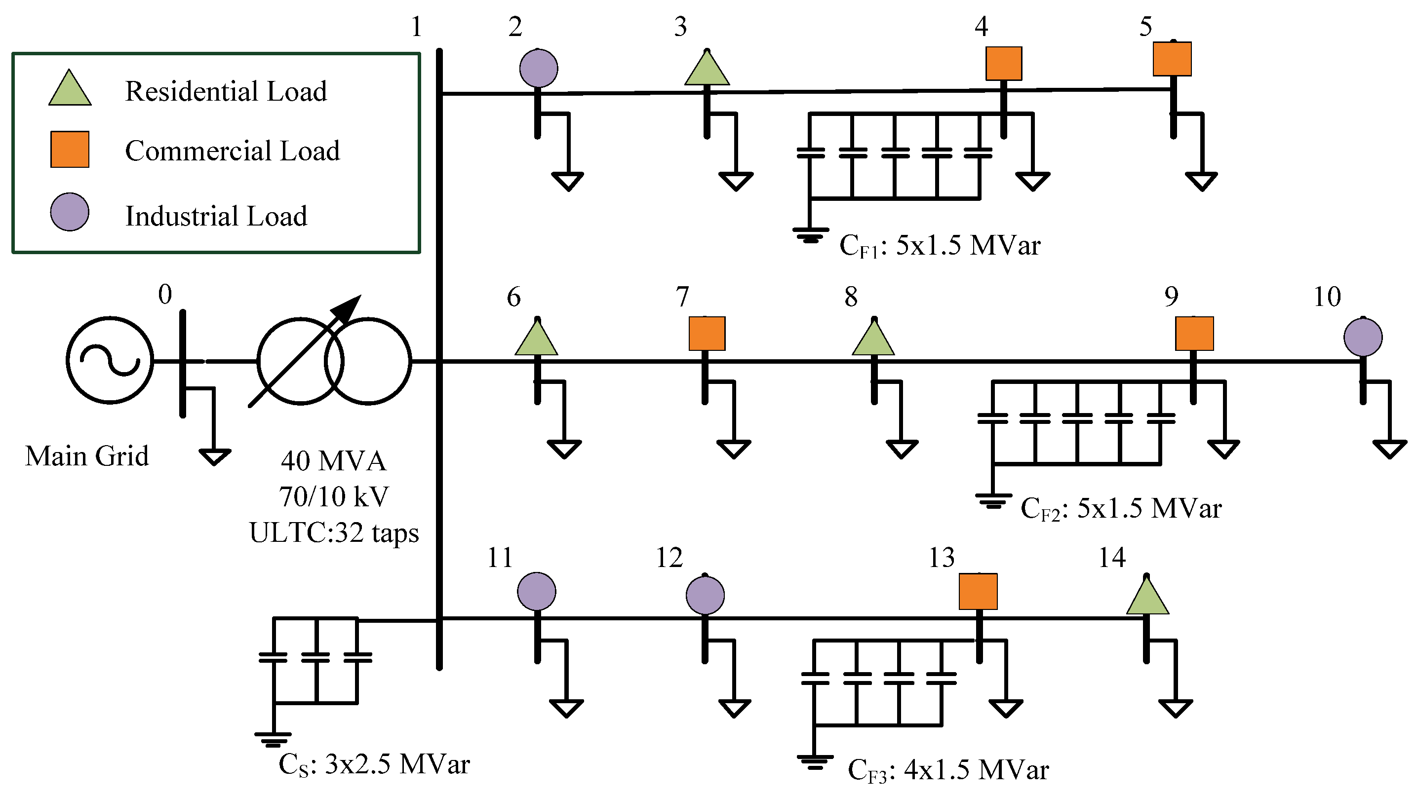
The remainder of the paper is organized as follows. Random matrix and data model in RPO are presented in Section 2. Section 3 presents the optimization formulation. Section 4 states the proposed method for predicting the reactive power adjustment. Results and comparisons are provided in Section 5 with the proposed method, using a real 10 kV distribution system. Section 6 summarizes main contributions and conclusions.

2. Random Matrix and Data Model in Reactive Power Optimization

2.1. Random Matrix of Loads

Large random matrix refers to the matrix including random numbers with part or all of that elements [18]. The loads change periodically in accordance with seasons, weeks and days, and it shows a random distribution feature with the influences of some factors, including weather condition, temperature, humidity, etc. It is feasible to construct a RM of load to analyze the varying patterns of load data.

RM of loads is defined as the one whose elements are nodal loads in power system. Assuming that the nodes number is N, the load data are sampled hourly, and the daily load curve can be expressed by a load vector with the size equaling to 24. Taking active power vector for an example, the daily load curve of the node i can be expressed by the vector ${\mathit{p}}_i$:

$${\mathit{p}}_i={(p_{i1},p_{i2},p_{i3},\cdot \cdot \cdot ,p_{i24})}^T$$

(1)

where $p_{i1}$, $p_{i2}$, $p_{i3}$,…, $p_{i24}$ denote the active power of the node i at 1:00, 2:00, 3:00, …, 24:00, respectively. For a network with N nodes, loads on all nodes can be expressed by a random matrix with $N\times 24$ dimensions, and the load random matrix of the active load can be expressed as:

$$P={[{\mathit{p}}_1,{\mathit{p}}_2,{\mathit{p}}_3,\cdot \cdot \cdot ,{\mathit{p}}_N]}^T$$

(2)

The reactive power vector of the node i can be expressed as ${\mathit{q}}_i={(q_{i1},q_{i2},q_{i3},\cdot \cdot \cdot ,q_{i24})}^T$, and the load random matrix of the reactive power can be expressed as:

$$Q={[q_1,{\mathit{q}}_2,{\mathit{q}}_3,\cdot \cdot \cdot ,{\mathit{q}}_N]}^T$$

(3)

2.2. Lengths and Covariance of Random Matrix of Loads

The norm of vector is important to measure the length of a vector. For a real vector $x={(x_1,x_2,x_3,\mathrm{...},x_m)}^T$, assuming its Euclid norm is expressed with d, then d can be expressed as:

$$d=\sqrt{{\displaystyle \sum _{i=1}^m{x}_i^2}}$$

(4)

In order to compare the similarity of different matrices, characteristics of the length, the distribution and the fluctuation of the matrices are measured. For the convenience of comparing the length of random load matrices, the length of a random matrix $X$ is defined as:

$$d=\sqrt{tr(X\cdot X^T)}$$

(5)

In Equation (5), tr(·) represents the trace of a matrix. The length of active power and the reactive power random matrix can be respectively expressed with $d_P$ and $d_Q$:

$$d_P=\sqrt{tr(P\cdot P^T)}$$

(6)

$$d_Q=\sqrt{tr(Q\cdot Q^T)}$$

(7)

In the multivariate statistics analysis, the sample covariance is usually essential when calculating some important statistics variables. The analysis of sample covariance is particularly important in multivariate statistics. Assuming vectors $x$, $y$ are two groups of random samples with Gaussian distributions, $x={(x_1,x_2,x_3,\mathrm{...},x_m)}^T$, $y={(y_1,y_2,y_3,\mathrm{...},y_m)}^T$, then the covariance of two vectors can be expressed as:

$$\mathrm{cov}(x,y)=\frac{1}{m}{\displaystyle \sum _{i=1}^m(x_i-\overline{x})}(y_i-\overline{y})$$

(8)

where $\overline{x}$, $\overline{y}$ are the average values of $x$, $y$, and $\overline{x}=\frac{1}{m}{\displaystyle \sum _{i=1}^m{x}_i}$, $\overline{y}=\frac{1}{m}{\displaystyle \sum _{i=1}^m{y}_i}$.

In order to compare the correlation between two random matrices, each matrix is treated as a extended vector in this paper. The covariance of matrices $A$ and $B$ is expressed by $\mathrm{cov}(A,B)$. Assuming matrices $A$, $B$ are $M\times N$ dimensions matrices and $A={\left\{a_{ij}\right\}}_{M\times N}$, $B={\left\{b_{ij}\right\}}_{M\times N}$, the covariance of $A$ and $B$ can be expressed as:

$$\mathrm{cov}(A,B)=\frac{1}{M\cdot N}{\displaystyle \sum _{i=1}^M{\displaystyle \sum _{j=1}^N(a_{ij}-\overline{a})}}(b_{ij}-\overline{b})$$

(9)

where $\overline{a}=\frac{1}{M\cdot N}{\displaystyle \sum _{i=1}^M{\displaystyle \sum _{j=1}^N{a}_{ij}}}$, $\overline{b}=\frac{1}{M\cdot N}{\displaystyle \sum _{i=1}^M{\displaystyle \sum _{j=1}^N{b}_{ij}}}$.

2.3. Data Model of Loads

Different load types are considered in establishing the load data model. The loads include three typical types, residential load type, commercial load type and industrial load type. In the process of data modeling, the original data are from real load data with hourly interval of Nantucket Electric Company [19]. The data are grouped with residential customer groups, commercial customer groups and industrial customer groups. The historical load data of three typical loads above from 2006 to 2014 are utilized to construct the simulation load data model.

The objective of RPO in operation period is to determine the proper action sequences of reactive power control devices one day ahead, based on load forecasting. Most studies on RPO treated load as simple or fixed typical load types based on the load forecasting of the day ahead. Loads in different seasons have different characteristics in the distribution and fluctuation of loads. Thus, the historical load data, the sequence adjustment operations of reactive power devices should be considered and utilized for the decision support of RPO. The daily load curves of residential load type, commercial load type and industrial load type are shown in Figure 1.

The load data model for big data RPO can be established based on the stored historical load data in DN. The daily load curves of the three kinds of load can be expressed with vectors $p_{\mathrm{Re}s}(t)$, $p_{Com}(t)$ and $p_{Ind}(t)$, as shown in Equation (10). The maximum allowable active load of node i is $p_{i,std}$ in a simulation case. The maximum loads of the three kinds of load in a year are $\text{max}(p_{\mathrm{Re}\mathrm{s}})$, $\text{max}(p_{Com})$, $\text{max}(p_{Ind})$. Then, the simulation load vector can be calculated as follows:

$$p_i(t)=\{\begin{array}{l}{p}_{i,std}\frac{p_{\mathrm{Re}\mathrm{s}}(t)}{\text{max}(p_{\mathrm{Re}s})}\begin{array}{cc},& for\hspace{1em}residential load\end{array}\\ p_{i,std}\frac{p_{Com}(t)}{\text{max}(p_{Com})}\begin{array}{cc},& for\hspace{1em}commercial load\end{array}\\ p_{i,std}\frac{p_{Ind}(t)}{\text{max}(p_{Ind})}\begin{array}{cc},& for\hspace{1em}industrial load\end{array}\end{array}$$

(10)

where $t=1,2,3,\mathrm{...},365$ for a year.

The active power in load random matrix is $P(t)={[{\mathit{p}}_1(t),{\mathit{p}}_2(t),{\mathit{p}}_3(t),\cdot \cdot \cdot ,{\mathit{p}}_N(t)]}^T$, and the reactive power in load random matrix is $Q(t)={[{\mathit{q}}_1(t),{\mathit{q}}_2(t),{\mathit{q}}_3(t),\cdot \cdot \cdot ,{\mathit{q}}_N(t)]}^T$.

2.4. Load Grouping

The daily load curves in different periods of a year have obviously different characters. A detailed grouping of the daily load curves considering characteristics in distribution and fluctuation can narrow the searching range and reduce time when comparing and matching loads in similarity. As shown in Figure 1, each line of daily load curves in different seasons greatly varies.

For residential load shown in Figure 1a, daily load curves in winter and spring appear two peaks and the evening peak appears 1 h earlier in winter than that in spring. In summer and autumn, there is one valley appeared between 2:00 and 7:00 a.m., and one peak between 5:00 and 10:00 p.m. The peak time lasts longer in summer than in autumn. For commercial load shown in Figure 1b, the peak time lasts longer in winter, from 8:00 a.m. to 8:00 p.m., than in spring from 9:00 a.m. to 5:00 p.m. Compared with load in winter and spring, the peak in summer and autumn is higher and it appears the highest in autumn. For industrial load shown in Figure 1c, the load in winter and spring share little fluctuation. The peak in summer and autumn appears from 9:00 a.m. to 9:00 p.m. Above all, the daily load curves can be separated into four types, spring load, summer load, autumn load and winter load, based on the different seasons.

Besides, daily load curves in workdays and weekends are different. Weekly load curves of residential load, commercial load and industrial load are shown in Figure 2. For residential load, load in weekend is a little lower than that in workday. While for commercial load and industrial load, load in weekend is obviously lower than that in workday. As the difference between loads in workday and weekend, daily load curves can be separated in two types, workday load and weekend load.

3. Problem Formulation

3.1. Overview

The day-ahead RPO problem can be defined as a dynamic optimization problem. The optimization objective is to minimize the total cost in the whole day of active power loss and the switching operation, while keeping no constraints violation. By solving the dynamic optimization, the optimal schedule in the coming day of switching device operation can be calculated one-day ahead.

3.2. Objective Function

The objective is to minimize the whole day’s active power loss at the same time ensuring that no constraint violations occur.

$$\begin{array}{c}\text{min}\hspace{1em}f(u)=\text{min}{\displaystyle \sum _{h=1}^{24}{P}_{Loss}^h}\\ P_{Loss}^h={\displaystyle \sum _{(i,j)\in B}{g}_{ij}\{{(V_i^h)}^2+{(V_j^h)}^2-2V_i^h{V}_j^h\cos {\theta }_{ij}\}}\end{array}$$

(11)

where $P_{Loss}^h$ is the power loss at time h, $B$ represents the set of branches, and $(i,j)\in B$ denotes the two nodes of one branch. $V_i^h$ and $V_j^h$ are voltage magnitudes of two nodes $i$ and $j$ at time h, respectively. $g_{ij}$ is the conductance value between nodes $i$ and $j$. ${\mathsf{\theta }}_{ij}$ is the phase angles difference of ${\mathsf{\theta }}_i$ and ${\mathsf{\theta }}_j$. $u$ is the vector containing all the control variables which is expressed as follow:

$$u=\{u^1,u^2,\cdot \cdot \cdot ,u^h,\cdot \cdot \cdot ,u^{24}\}$$

(12)

where $u^h$ is the vector of RPO control variables at time h, which is expressed as follow:

$$u^h=(Q_{\mathrm{c}1}^h,Q_{\mathrm{c}2}^h,\cdot \cdot \cdot ,Q_{\mathrm{c}{N}_c}^h,T_{\mathrm{r}1}^h,T_{\mathrm{r}2}^h,\cdot \cdot \cdot ,T_{\mathrm{r}{N}_r}^h)$$

(13)

where $Q_{\mathrm{c}i}^h$ and $T_{\mathrm{r}i}^h$ are the compensation capacity of reactive power capacitor and the tap setting of regulating transformer at time h, respectively. $N_{\mathrm{c}}$ is the number of the compensator capacitors including substation capacitors and feeder capacitors. $N_{\mathrm{r}}$ is the number of regulating transformers. The vector of state variables x is expressed as follow:

$$x=\{x^1,x^2,\cdot \cdot \cdot ,x^h,\cdot \cdot \cdot ,x^{24}\}$$

(14)

where $x^h$ is the vector of state variables at time h, which is expressed as follow:

$$x^h=(V_1^h,V_2^h,\cdot \cdot \cdot ,V_N^h,{\theta }_1^h,{\theta }_2^h,\cdot \cdot \cdot ,{\theta }_N^h)$$

(15)

where $N$ is the total number of nodes.

3.3. Constraints

3.3.1. Equality Constraints

The constraint of power flow can be expressed as:

$$\begin{array}{l}{P}_{DGi}-P_{di}=V_i{\displaystyle \sum _{j=1}^N{V}_j(G_{ij}\cos {\mathsf{\theta }}_{ij}+B_{ij}\sin {\mathsf{\theta }}_{ij})} \\ Q_{DGi}-Q_{di}=V_i{\displaystyle \sum _{j=1}^N{V}_j(G_{ij}\sin {\mathsf{\theta }}_{ij}-B_{ij}\cos {\mathsf{\theta }}_{ij})} \end{array}$$

(16)

where $P_{DGi}$ and $Q_{DGi}$ are active and reactive generation outputs, respectively; $P_{di}$ and $Q_{di}$ are active/reactive loads at node $i$, respectively; and $G_{ij}$ and $B_{ij}$ are the real/imaginary parts of the nodal admittance matrix, respectively.

3.3.2. Inequality Constraints

Reactive power limits of capacitors:

$$Q_{\mathrm{c}i}^{\text{min}}\le Q_{\mathrm{c}i}^h\le Q_{\mathrm{c}i}^{\text{max}}i=1,\mathrm{...},N_c$$

(17)

Switching operations constraints:

$$T_{\mathrm{r}i}^{\text{min}}\le T_{\mathrm{r}i}^h\le T_{\mathrm{r}i}^{\text{max}}i=1,\mathrm{...},N_{\mathrm{r}}$$

(18)

Nodal voltage constraints:

$$V_i^{\text{min}}\le V_i^h\le V_i^{\text{max}}i=1,\mathrm{...},N$$

(19)

where $Q_{\mathrm{c}}^{\text{min}}$ and $Q_{\mathrm{c}}^{\text{max}}$ are the minimum and maximum compensation capacity of reactive power capacitor, respectively. $T_{\mathrm{r}}^{\text{min}}$ and $T_{\mathrm{r}}^{\text{max}}$ are lower/upper tap setting of regulating transformers, respectively. $V_i^{\text{min}}$ and $V_i^{\text{max}}$ are the minimum and maximum limits of voltage magnitude in 24 h at node i, respectively.

3.3.3. Constraints on Equipment Operations Number

Since the compensator capacitors and tap setting of regulating transformers are discrete values, there are operations limits in order to prolong equipment life. The equipment operations number constraints are as follows:

$${\displaystyle \sum _{h=1}^{23}\left|Q_{\mathrm{c}}^h-Q_{\mathrm{c}}^{h+1}\right|}\le C_{\mathrm{c}}$$

(20)

$${\displaystyle \sum _{h=1}^{23}\left|T_{\mathrm{r}}^h-T_{\mathrm{r}}^{h+1}\right|}\le C_{\mathrm{r}}$$

(21)

where $C_{\mathrm{c}}$ and $C_{\mathrm{r}}$ are the operations limit of compensator capacitors and tap setting of regulating transformers, respectively.

3.4. Overall Formulation

The control variables of RPO problem include the compensator capacitors at load buses $Q_{\mathrm{c}}$, tap setting of regulating transformers units $T_{\mathrm{r}}$. The status variables include the nodal voltage $V$, nodal voltage phase angle $\theta$, etc. Taking the objectives and constraints into consideration, the RPO problem can be expressed as follows:

$$\text{min}{P}_{\mathrm{loss}}=f\left(\mathit{u},\mathit{x}\right)$$

(22)

$$\begin{array}{cc}s.t.& g_{eq}\left(\mathit{u},\mathit{x}\right)\end{array}=0$$

(23)

$$g_L\le g_{neq}\left(\mathit{u},\mathit{x}\right)\le g_U$$

(24)

4. The Proposed Method for Predicting the Reactive Power Adjustment

4.1. Sensitivity Analysis

Sensitivity analysis is one of the commonly used power system analysis methods, based on the power flow constraints and reflecting the mutual influence between variables by differentiation relations. Compared with traditional analysis methods, it has advantages in power system analysis. It transforms inter bus P-Q-V relationships into an easier form to make decisions [20]. To calculate the active power loss sensitivity to the reactive power control variable, define the power flow constraint to be generalized as:

$$g(\mathit{u},\mathit{v})=0$$

(25)

The total daily active power loss can be generalized as:

$$P_{\mathrm{loss}}=f(\mathit{u},\mathit{v})$$

(26)

When the control variable increment $\Delta \mathit{u}$ and the state variable increment are small, the quadratic and higher terms in the Taylor expandable of Equation (25) can be ignored. The increment of $g(\mathit{u},\mathit{v})$ can be approximately expressed as:

$$\Delta g=\frac{\partial g}{\partial \mathit{u}}\Delta \mathit{u}+\frac{\partial g}{\partial \mathit{x}}\Delta \mathit{x}$$

(27)

Let $\Delta g=0$, the state variable increment can be expressed as:

$$\Delta \mathit{x}=-{\left(\frac{\partial g}{\partial \mathit{x}}\right)}^{-1}\frac{\partial g}{\partial \mathit{u}}\Delta \mathit{u}$$

(28)

The total daily active power loss increment can be formulated as:

$$\Delta P_{\mathrm{loss}}=\frac{\partial f}{\partial \mathit{u}}\Delta \mathit{u}+\frac{\partial f}{\partial \mathit{x}}\Delta \mathit{x}$$

(29)

Combining Equation (28) and Equation (29) yields the total daily active power loss increment:

$$\Delta P_{\mathrm{loss}}=\left[\frac{\partial f}{\partial \mathit{u}}-\frac{\partial f}{\partial \mathit{x}}{\left(\frac{\partial g}{\partial \mathit{x}}\right)}^{-1}\frac{\partial g}{\partial \mathit{u}}\right]\Delta \mathit{u}$$

(30)

Then, the active power loss sensitivity to the control variable can be expressed as:

$$S_u=\frac{\partial f}{\partial \mathit{u}}-\frac{\partial f}{\partial \mathit{x}}{\left(\frac{\partial g}{\partial \mathit{x}}\right)}^{-1}\frac{\partial g}{\partial \mathit{u}}$$

(31)

4.2. Load Similarity

In the same period of different years, the daily load curves are similar. To measure the similarity of forecasting load and the historical load quantitatively, load similarity (LS) is defined to measure the similarity level of the length quantitatively. To reflect the fluctuation of daily load cures in the same network of two days, the load similarity s is defined.

According to Equations (2) and (3), the historical load and forecasting load of the day ahead can be represented with random matrix. $P_H$ and $Q_H$, respectively, represent the historical active load and reactive load. $P_F$ and $Q_F$, respectively, represent the active load and reactive load of the day ahead. Structure the load augmented matrix $A_H=\left[\begin{array}{l}{P}_H\\ Q_H\end{array}\right]$, $A_F=\left[\begin{array}{l}{P}_F\\ Q_F\end{array}\right]$ Combining with the method to obtain the length of the matrix in Equation (5) and the method to obtain the covariance of random matrix in Equation (9), the load similarity can be listed as:

$$s=\left(1-\frac{\left|d_{A_H}-d_{A_F}\right|}{d_{A_H}+d_{A_F}}\right)\frac{\mathrm{cov}(A_H,A_F)}{\sqrt{\mathrm{cov}(A_H,A_H)}\cdot \sqrt{\mathrm{cov}(A_F,A_F)}}$$

(32)

where $0\le 1-\frac{\left|d_{A_H}-d_{A_F}\right|}{d_{A_H}+d_{A_F}}\le 1$, $-1\le \frac{\mathrm{cov}(A_H,A_F)}{\sqrt{\mathrm{cov}(A_H,A_H)}\cdot \sqrt{\mathrm{cov}(A_F,A_F)}}\le 1$, so the load similarity ranges from –1 to 1. As load similarity $s$ approaches 1, the similarity of matrix $A_H$ and $A_F$ rises, indicating the similarity of historical load and forecasting load rises. Only when $A_H=A_F$, load similarity is $s=1$, indicating historical load and forecasting load are the same.

4.3. Reactive Power Optimization Method Based on Big Data

The big data reactive power optimization (BDO) method presented in this paper is targeted to solve the dynamic RPO problem in distribution network. It optimizes dispatching scheme of reactive power control devices of the day ahead, based on forecasting load, reducing active power losses and making voltage quality better. Compared with the traditional optimization method based on exact mathematical models, the big data RPO method relies on the historical RPO empirical data. By calculating the load similarity between the forecasting load random matrix and the historical load random matrix, dispatching scheme of the day ahead can be obtain from the best matching historical RPO dispatching scheme.

4.3.1. Data Preparation

(a) Obtain the forecasting load data of the day ahead and establish the forecasting load random matrix $P_F$, $Q_F$ according to Equations(2) and (3). Then, establish the forecasting load augmented matrix $A_F$.

(b) Obtain the historical load data of the distribution network in recent years and establish the historical load augmented matrix $A_H(t)$ of each day, where $t=1,2,3,\cdot \cdot \cdot ,L$ and L stands for the total number of days. Then, obtain the reactive power control devices dispatching scheme of each day, including the sequence of tap settings and the sequence of capacitor capacities in 24 h.

(c) Divide the historical load augmented matrices into four groups according to seasons, as shown in Figure 3. Then, divide the historical load augmented matrices for each season into two subgroups, workdays and weekends; not that holidays are treated as weekends. Define $\mathsf{\lambda }$ as the seasonal grouping property and $\mathsf{\mu }$ as weekday grouping property. Define $c(\mathsf{\lambda },\mathsf{\mu })$ as the subset of t after the grouping according to Figure 3. The groups of load are shown in

Table 1. Groups of load.

$c(\mathsf{\lambda },\mathsf{\mu })$	Workday, $\mathsf{\mu }=1$	Weekend, $\mathsf{\mu }=1$
Spring, $\mathsf{\lambda }=1$	$t\in c(1,1)$	$t\in c(1,2)$
Summer, $\mathsf{\lambda }=2$	$t\in c(2,1)$	$t\in c(2,2)$
Autumn, $\mathsf{\lambda }=3$	$t\in c(3,1)$	$t\in c(3,2)$
Winter, $\mathsf{\lambda }=4$	$t\in c(4,1)$	$t\in c(4,2)$

.

4.3.2. Load Similarity Matching

The big data RPO method is presented in detail as follows:

Step 1: Establish the forecasting load augmented matrix of the day ahead, based on the forecasting load. According to the date of the day ahead, determine the load grouping properties $\mathsf{\lambda }$ and $\mathsf{\mu }$.

Step 2: Based on grouping properties, select the group $t\in c(\mathsf{\lambda },\mathsf{\mu })$ and establish the corresponding historical load augmented matrices $A_H(t)$, where $t\in c(\mathsf{\lambda },\mathsf{\mu })$.

Step3: According to Equation (32), calculate the load similarity $s(t)$ of historical load augmented matrix $A_H(t)$ and forecasting load augmented matrix $A_F$, when $t\in c(\mathsf{\lambda },\mathsf{\mu })$.

Step 4: According to Equation (33), the best matching day $t=t_{\text{max}}$ can be found when the load similarity becomes the maximum.

$$s(t_{\text{max}})=\text{max}[s(t)], t\in c(\mathsf{\lambda },\mathsf{\mu })$$

(33)

Step 5: Set the minimum load similarity margin $s_{\text{min}}$ based on experience.

Step 6: Compare the largest load similarity $s(t_{\text{max}})$ with the minimum load similarity margin $s_{\text{min}}$.

Step 7: If $s(t_{\text{max}})\ge s_{\text{min}}$, the historical load of the day with date $t=t_{\text{max}}$ and forecasting load have high similarity. The reactive power control devices dispatching scheme can be obtained from the historical sequence of tap setting and sequence of compensation capacity.

Step 8: If $s(t_{\text{max}})\le s_{\text{min}}$, the historical load of the day with date $t=t_{\text{max}}$ and forecasting load have low similarity. The reactive power control devices dispatching scheme of the day ahead should be calculated with a fine adjustment method based on sensitivity analysis.

Step 9: Store the RPO data into database including the forecasting load and the reactive power control devices dispatching scheme.

The flow diagram of the big data RPO method is shown in Figure 4.

4.3.3. Fine Adjustment Method Based on Sensitivity Analysis

When the load similarity between the forecasting load augmented matrix $A_F$ and the historical load augmented matrix $A_H$ is smaller than the minimum load similarity margin $s_{\text{min}}$, the reactive power control devices dispatching scheme cannot be achieved by the load similarity matching directly. Then, a fine adjustment method based on sensitivity analysis is required because the forecasting load and the historical load share little similarity. Based on Equation (31), the total daily active power loss sensitivity to the control variable can be achieved. To reduce the total daily active power loss, the increment should satisfy the constraint $\Delta P_{\mathrm{loss}}<0$ during the fine adjustment processes. According to Equation (30), the sensitivity and control variable increment should satisfy the following inequalities constraints:

$$\{\begin{array}{l}{S}_u<0,\Delta \mathit{u}>0\\ S_u>0,\Delta \mathit{u}<0\end{array}$$

(34)

Based on Equation (34), in order to adjust the action moment of the control devices only without increasing the actions of the control devices, the control variable increment can be calculate according to Algorithm 1.

Algorithm 1. Control variable increment calculation rules
if the sensitivity of active loss to control variable $S_u<0$
	if $u^h>u^{h+1}$ or $u^h>u^{h-1}$
		control variable increment $\Delta u^h=\text{max}(u^{h+1},u^{h-1})-u^h$
	end if
else if the sensitivity of active loss to control variable $S_u>0$
	if $u^h<u^{h+1}$ or $u^h<u^{h-1}$
		control variable increment $\Delta u^h=\text{min}(u^{h+1},u^{h-1})-u^h$
	end if
Else control variable increment $\Delta u^h=0$
end if

With the control variable increment calculation rules, the control variable fine adjustment method can be presented as follow:

Step 1: According to reactive power control devices dispatching scheme achieved by load similarity matching, initialize the control variable $u_k^h$, where $h=1,2,3,\mathrm{...},24$. Let the iteration number k = 1.

Step 2: Calculate the reactive power loss $P_{loss,k}$ when the control variable is $u_k^h$.

Step 3: Calculate the active power loss sensitivity $S_{u,k}$ to the control variable.

Step 4: According to the control variable increment calculation rules, calculate the control variable increment $\Lambda u_k^h$.

Step 5: Update the control variable by $u_{k+1}^h=u_k^h+\Delta u_k^h$ and calculate the new active power loss $P_{loss,k+1}$.

Step 6: If $P_{\mathrm{loss},k+1}<P_{\mathrm{loss},k}$, let k = k + 1 and continue the iteration process to Step 3. Otherwise, output the final control variable $u_k^h$.

The computing flow chart of the he control variable $u_k^h$ is shown in Figure 5.

5. Experiments and Results

5.1. Experiments Setting and Descriptions

To obtain the effectiveness of the proposed method, a standard DN test system is chosen to test based on [21]. The single-line diagram of the DN test system is shown in Figure 6. There are 14 nodes in this system with three feeders. The reactive power devices are one ULTC, one substation capacitor and three feeder capacitors in the system, whose configuration information is shown in

Table 2. Configuration of reactive power devices.

Device	Setting
ULTC	70/10 kV, −10% to 10% regulation with 32 steps
CS	Substation capacitors: 2.5 Mvar each
CF	Feeder capacitors: 1.5 Mvar each

.

In the test system, the nodes are separated into three types, residential load type, commercial load type and industrial load type (

Table 3. Load types.

Load Type	Node
Residential load	3, 6, 8, 14
Commercial load	4, 5, 7, 9, 13
Industrial load	2, 10, 11, 12

). The historical load data used in the test are from practical hourly load data collected by Nantucket Electric Company. Based on the load data model presented in Section 2, the simulation load data are established with the practical load for nine years from 2006 to 2014 according to Equation (10). The data of the years from 2006 to 2013 are treated as historical load. Suppose load forecasting has been accurately completed and ignore the load forecasting deviation. The data of 2014 can be used to test the method. An improved multi-population genetic algorithm (MGA) is chosen to obtain the historical RPO dispatching scheme based on the simulation load. Then, the history data including the sequence of tap setting actions and capacitor capacities are available.

5.2. Experiment on Standard Test Case

5.2.1. Calculation of Minimum Load Similarity Margin

The minimum load similarity margin $s_{\text{min}}$ is a parameter to affect the similarity matching accuracy. To determine $s_{\text{min}}$, 365 load matrices of one year are chosen to be tested. Define $P_{lossMGA}$ as the active power loss after optimized by the MGA method and $P_{lossBDO}$ as that after optimized by the BDO method without fine adjustment. To compare the active power losses of two methods, a factor named loss error is defined as follow:

$$err=\frac{P_{lossBDO}-P_{lossMGA}}{P_{lossMGA}}\times 100\%$$

(35)

Figure 7 shows the distribution of load similarity and loss error. As seen from Figure 7, the loss errors are consistently lower than 1%. Most of the points are centralized at the sector area divided by the two lines through point (0, 1). The point distributions approach high density when close to point (0, 1). As shown on Figure 7, the loss errors are lower than 0.5% when the load similarities are larger than 0.95. Twenty groups of optimization results are shown in

Table 4. Optimization result of MGA (multi-population genetic algorithm) and BDO (big data reactive power optimization) without fine adjustment.

No.	Loss of MGA (MWh)	Loss of BDO (MWh)	Similarity	Error (%)
1	7.9886	7.9971	0.9741	0.1074
2	7.8271	7.8406	0.8888	0.1734
3	15.3140	15.3225	0.9779	0.0561
4	8.5332	8.5356	0.9618	0.0282
5	7.1424	7.1453	0.9731	0.0408
6	11.5872	11.6022	0.9595	0.1288
7	7.4006	7.4100	0.9332	0.1268
8	15.1935	15.2026	0.9780	0.0599
9	8.6196	8.6207	0.9856	0.0131
10	14.0853	14.0928	0.9857	0.0529
11	8.9968	8.9973	0.9557	0.0054
12	8.7716	8.7723	0.9597	0.0080
13	10.5138	10.5196	0.9754	0.0551
14	7.0980	7.0980	0.9688	0.0000
15	7.3734	7.3806	0.9382	0.0976
16	6.6822	6.6869	0.9509	0.0700
17	9.0290	9.0409	0.9552	0.1311
18	9.4201	9.4521	0.9515	0.3393
19	8.9582	8.9799	0.9665	0.2428
20	8.0961	8.1206	0.9350	0.3029

. Compared with the optimization result of MGA, the active power losses of BDO are larger than those of MGA, but the loss errors are lower than 1%, which is acceptable. Thus, the minimum load similarity margin can be set to 0.95 in this paper.

5.2.2. Three test cases

Case 1: Test of a Random Day

A workday in summer with heavy load is chosen to be tested. During the experiment procedure, we set the load property $\mathsf{\lambda }=2$ for summer, $\mathsf{\mu }=1$ for workday and the minimum load similarity margin $s_{\text{min}}=0.95$.

During the experiment, the maximum load similarity is $s(t_{\text{max}})=0.9684>s_{\text{min}}$, so the historical RPO dispatching scheme of date $t_{\text{max}}$ can be used on the tested day without fine adjustment.

Most of the reactive power control device action sequences by BDO and MGA are the same, except some actions of C_F1 and C_F2 at several points shown in Figure 8a,b. The optimization results of the selected day are shown in

Table 5. Optimization results of a random day.

Optimization Method	Action Times					Loss (MWh)	Computing Time (s)
	ULTC	CS	CF1	CF2	CF3
MGA	4	2	2	2	2	14.4631	141.6
BDO	4	2	1	2	2	14.4805	0.283

.

Based on the results of BDO and MGA, as shown in Table 5, the comparison of the two methods can be presented as follows. In the aspect of active power loss, the BDO method achieves a little larger active power loss than the MGA method. The loss error is 2.76%, which is acceptable in engineering application under undemanding condition. In the aspect of device action times, the BDO method can spend less action times than the MGA method, which can prolong the service life of the devices. In the aspect of computation time, the BDO method can achieve the optimization result within 0.5 s, while the computation time of MGA method lasts as long as 141.6 s. It is concluded that the BDO method can be a fast RPO method.

Comparing the optimization results of BDO method and MGA method, the differences appear at the feeder capacitor units C_F1 and C_F2, as shown in Figure 8a,b. The BDO method shows less action times at C_F1 and presents less compensation capacity at C_F2 compared with the MGA method.

Case 2: Test of Some Random Days

In order to compare performances of BDO and MGA, 20 random days are chosen to be tested. The optimization results are shown in

Table 6. Optimization results of 20 random days.

No.	Load Similarity	$s(t_{\text{max}})\ge s_{\text{min}}$	Loss (MWh)			Loss Error (%)	Computing Time (s)
			MGA	BDO (a)	BDO (b)		MGA	BDO
1	0.9657	Yes	7.2708	7.2710	-	0.0020	138.91	0.2473
2	0.9682	Yes	7.3735	7.3747	-	0.0153	133.34	0.2810
3	0.9536	Yes	7.8297	7.8472	-	0.2241	155.77	0.2966
4	0.9332	No	7.4009	7.4017	7.4012	0.0048	155.51	0.3130
5	0.9465	No	7.4885	7.4908	7.4897	0.0162	108.40	0.3263
6	0.9668	Yes	6.1113	6.1120	-	0.0127	141.80	0.2826
7	0.9797	Yes	7.3538	7.3563	-	0.0334	136.40	0.2353
8	0.9787	Yes	8.0612	8.0658	-	0.0581	168.11	0.2577
9	0.9670	Yes	9.4710	9.4823	-	0.1193	186.73	0.2482
10	0.9264	No	13.3107	13.3258	13.2658	−0.3370	187.37	0.3505
11	0.9852	Yes	14.9465	14.9511	-	0.0304	108.45	0.2615
12	0.9796	Yes	13.0150	13.0156	-	0.0046	146.09	0.3024
13	0.9358	No	14.7954	14.8173	14.7873	−0.0550	94.44	0.2742
14	0.9399	No	8.6167	8.6319	8.6119	−0.0546	98.46	0.3067
15	0.9783	Yes	9.6760	9.6763	-	0.0030	142.73	0.2571
16	0.9802	Yes	9.0971	9.1012	-	0.0456	204.31	0.2379
17	0.9509	Yes	6.6868	6.6906	-	0.0571	112.21	0.2373
18	0.9765	Yes	8.3112	8.3162	-	0.0599	157.86	0.2946
19	0.9632	Yes	10.3017	10.3087	-	0.0674	133.98	0.2747
20	0.9765	Yes	6.9651	6.9654	-	0.0045	187.69	0.2741

, in which the losses of BDO (a) and BDO (b) stand for the losses before and after the application of control variables fine adjustment method, respectively.

As shown in Table 6, there are five days requiring fine adjustment with similarities smaller than 0.95 and another 15 days obtaining the optimization results simply by similarity matching. The largest loss error is 0.2241%, which means the BDO method can obtain a similar result to the MGA method. There are negative loss errors, which mean the BDO method may obtain a more excellent result than the MGA method.

Case 3: Test of Typical Days

Based on the load grouping process shown in Figure 3, typical days of different categories are chosen to be tested among workdays and weekends in different seasons. Both the BDO method and the MGA method are used to obtain the optimization results. As shown in

Table 7. Optimization results of typical days.

Load Property	Forecasting Date	Historical Date	Load Similarity	Loss (MWh)
				BDO	MGA
Workday, spring	17 March 2014	5 March 2012	0.9576	7.0678	6.8871
Weekend, spring	16 March 2014	7 April 2013	0.9618	6.1504	6.0030
Workday, summer	18 June 2014	10 June 2013	0.9644	16.1209	15.7828
Weekend, summer	15 June 2014	7 July 2013	0.9531	14.7790	14.3192
Workday, autumn	15 September 2014	13 September 2011	0.9701	12.9096	12.7573
Weekend, autumn	14 September 2014	15 September 2012	0.9665	12.4243	12.1118
Workday, winter	17 December 2014	9 December 2009	0.9636	7.8655	7.6621
Weekend, winter	14 December 2014	16 December 2012	0.9547	6.1919	5.8347

, though the losses by the BDO method are a little larger than those by the MGA method, it is acceptable within the range of allowable error. The dates of matched historical day are in a range of the nearest five years, which means we can select historical data of only the last five years when choosing historical data.

6. Conclusions

A fast RPO method based on historical data is presented. The proposed method is tested on a DN, and comparison has been made with a MGA method. The experimental result proves that the RPO method is an effective and feasible method within the range of allowable deviations. The contribution and the novelties of the proposed method can be generalized as:

(1) The proposed novel RPO method is robust and fast. The method has better feasibility than stochastic searching method.

(2) It is suitable for fast RPO in distribution network, which has enough historical RPO data. As the same time, it is unsuitable for a new network without historical data. Network topology structure is also assumed to be invariant.

References

1. Aoki, K.; Fan, W.; Nishikori, A. Optimal VAR planning by approximation method for recursive mixed-integer linear programming. IEEE Trans. Power Syst. 1988, 3, 1741–1747. [Google Scholar] [CrossRef]
2. Ferreira, R.S.; Borges, C.L.; Pereira, M.V. A flexible mixed-integer linear programming approach to the AC optimal power flow in distribution systems. IEEE Trans. Power Syst. 2014, 29, 2447–2459. [Google Scholar] [CrossRef]
3. Iba, K. Reactive power optimization by genetic algorithm. IEEE Trans. Power Systems 1994, 9, 685–692. [Google Scholar] [CrossRef]
4. Urdaneta, A.J.; Gomez, J.F.; Sorrentino, E.; Flores, L.; Diaz, R. A hybrid genetic algorithm for optimal reactive power planning based upon successive linear programming. IEEE Trans. Power Syst. 1999, 14, 1292–1298. [Google Scholar] [CrossRef]
5. Zhao, J.Q.; Ju, L.J.; Dai, Z M.; Chen, G. Voltage stability constrained dynamic optimal reactive power flow based on branch-bound and primal-dual interior point method. Int. J. Electr. Power Energy Syst. 2015, 73, 601–607. [Google Scholar] [CrossRef]
6. Sheng, W.; Liu, K.-Y.; Cheng, S. Optimal power flow algorithm and analysis in distribution system considering distributed generation. IET Gener. Transm. Distrib. 2014, 8, 261–272. [Google Scholar] [CrossRef]
7. Ding, T.; Liu, S.; Yuan, W.; Bie, Z.; Zeng, B. A Two-Stage Robust Reactive Power Optimization Considering Uncertain Wind Power Integration in Active Distribution Networks. IEEE Trans. Sustain. Energy 2016, 7, 301–311. [Google Scholar] [CrossRef]
8. Liu, L.; Li, H.; Xue, Y.; Liu, W. Reactive power compensation and optimization strategy for grid-interactive cascaded photovoltaic systems. IEEE Trans. Power Electron. 2015, 30, 188–202. [Google Scholar]
9. He, X.; Ai, Q.; Qiu, R.C.; Huang, W.; Piao, L.; Liu, H. A Big Data Architecture Design for Smart Grids Based on Random Matrix Theory. IEEE Trans. Smart Grid. 2015, in press. [Google Scholar]
10. Silverstein, J.; Combettes, P. Signal detection via spectral theory of large dimensional random matrices. IEEE Trans. Signal Process. 1992, 40, 2100–2105. [Google Scholar]
11. Frisch, A.; Mark, M.; Aikawa, K.; Ferlaino, F.; Bohn, J.L.; Makrides, C.; Petrov, A.; Kotochigova, S. Quantum chaos in ultracold collisions of gas-phase erbium atoms. Nature 2014, 507, 475–479. [Google Scholar] [CrossRef] [PubMed]
12. Hassan, M.; Bermak, A. Robust Bayesian Inference for Gas Identification in Electronic Nose Applications by Using Random Matrix Theory. IEEE Sens. J. 2016, 16, 2036–2045. [Google Scholar] [CrossRef]
13. Couillet, R.; Hachem, W. Fluctuations of spiked random matrix models and failure diagnosis in sensor networks. IEEE Trans. Inf. Theory 2013, 59, 509–525. [Google Scholar] [CrossRef]
14. Nobi, A.; Maeng, S.E.; Ha, G.G.; Lee, J.W. Random matrix theory and cross-correlations in global financial indices and local stock market indices. J. Kor. Phys. Soc. 2013, 62, 569–574. [Google Scholar] [CrossRef]
15. Manyika, J.; Chui, M.; Brown, B. Big data: The Next Frontier for Innovation, Competition, and Productivity; The McKinsey Global Institute: Las Vegas, NV, USA, 2014. [Google Scholar]
16. Yin, J.; Sharma, P.; Gorton, I.; Akyoli, B. Large-scale data challenges in future power grids. In Proceedings of the 2013 IEEE 7th International Symposium on Service Oriented System Engineering (SOSE), Redwood City, CA, USA, 25–28 March 2013; pp. 324–328.
17. Kezunovic, M.; Xie, L.; Grijalva, S. The role of big data in improving power system operation and protection. In Proceedings of the 2013 IEEE IREP Symposium on Bulk Power System Dynamics and Control-IX Optimization, Security and Control of the Emerging Power Grid (IREP), Rethymno, Greece, 25–30 August 2013.
18. Wigner, E.P. Characteristic vectors of bordered matrices with infinite dimensions I. In The Collected Works of Eugene Paul Wigner; Springer-Berlin: Heidelberg, Germany, 1993; pp. 524–540. [Google Scholar]
19. National Grid. Available online: http://www.nationalgridus.com/energysupply/data.asp (accessed on 2 December 2015).
20. Tamp, F.; Ciufo, P. A Sensitivity Analysis Toolkit for the Simplification of MV Distribution Network Voltage Management. IEEE Trans. Smart Grid. 2014, 5, 559–568. [Google Scholar] [CrossRef]
21. Kim, Y.; Ahn, S.; Hwang, P.; Pyo, G.; Moon, S. Coordinated Control of a DG and Voltage Control Devices Using a Dynamic Programming Algorithm. IEEE Trans. Power Syst. 2013, 28, 42–51. [Google Scholar] [CrossRef]
Figure 1. Three types of typical daily load curves in different seasons: (a) residential load; (b) commercial load; and (c) industrial load.
Applsci 06 00158 g001aApplsci 06 00158 g001b
Figure 2. Three types of typical weekly load curves.
Applsci 06 00158 g002
Figure 3. Load grouping process.
Applsci 06 00158 g003
Figure 4. Fine adjustment method based on sensitivity analysis.
Applsci 06 00158 g004
Figure 5. Flow chart of control variable fine adjustment method.
Applsci 06 00158 g005
Figure 6. Test case of standard 14-node system.
Applsci 06 00158 g006
Figure 7. Distribution of load similarity and loss error.
Applsci 06 00158 g007
Figure 8. Capacities of capacitor units of different methods: (a) capacitor unit CF1 at Node 4; and (b) capacitor unit CF2 at Node 9.
Applsci 06 00158 g008