
The Spotting Distribution of Wildfires

Centre for Mathematical Biology, Department of Mathematical and Statistical Sciences, University of Alberta, Edmonton, AB T6G2G1, Canada
*
Author to whom correspondence should be addressed.
Appl. Sci. 2016, 6(6), 177; https://0-doi-org.brum.beds.ac.uk/10.3390/app6060177
Submission received: 12 February 2016
/
Revised: 11 May 2016
/
Accepted: 23 May 2016
/
Published: 17 June 2016
(This article belongs to the Special Issue Dynamical Models of Biology and Medicine)
Abstract
:In wildfire science, spotting refers to non-local creation of new fires, due to downwind ignition of brands launched from a primary fire. Spotting is often mentioned as being one of the most difficult problems for wildfire management, because of its unpredictable nature. Since spotting is a stochastic process, it makes sense to talk about a probability distribution for spotting, which we call the spotting distribution. Given a location ahead of the fire front, we would like to know how likely is it to observe a spot fire at that location in the next few minutes. The aim of this paper is to introduce a detailed procedure to find the spotting distribution. Most prior modelling has focused on the maximum spotting distance, or on physical subprocesses. We will use mathematical modelling, which is based on detailed physical processes, to derive a spotting distribution. We discuss the use and measurement of this spotting distribution in fire spread, fire management and fire breaching. The appendix of this paper contains a comprehensive review of the relevant underlying physical sub-processes of fire plumes, launching fire brands, wind transport, falling and terminal velocity, combustion during transport, and ignition upon landing.
1. Introduction
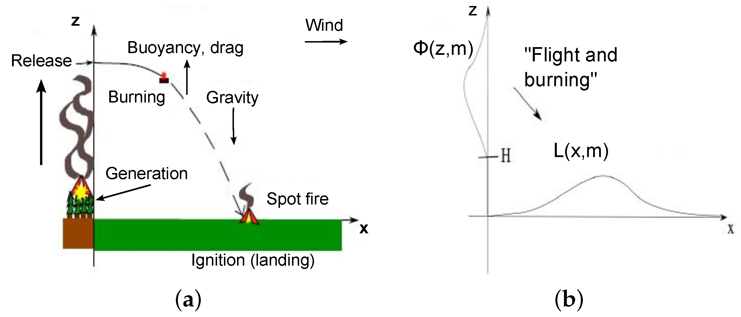
Wildfires are capable of creating powerful updrafts, called convection columns, which launch burning plant materials—referred to as firebrands—into the atmosphere [1]. Generally one speaks of coupled fire-atmosphere interactions [2], in which heat and moisture exchanges occur between the fire, the convection column and the atmosphere, resulting in the birth of new fire-driven wind and convective updrafts. Firebrands are then transported by the ambient windflow, simultaneously combusting and decreasing in mass, until they reach the ground. Upon landing, depending on the local fuel and weather conditions at the landing site, a firebrand may ignite the local fuel and start a new fire. Such a fire is called a spot fire, and the process is called spotting (see Figure 1a for a sketch of the spotting process). Spotting occurs in many ecosystems spanning the Earth, from the Americas to Europe, Africa and Australia.
Spotting can play an important role in wildfire spread, and while many of the subprocesses outlined in Figure 1 have been studied in detail, many remain poorly understood. One thing is certain: where spotting is important, it is a very diffficult spread mechanism to understand and therefore control.
The model framework we present here has the potential to produce realistic spotting distributions: spatial maps describing the probability of spot fires downwind of an existing fire. We will show how it is possible to incorporate the vast, but disparate literature on spotting, with some new ideas, to create a very robust modelling framework. We hope to draw the interest of researchers, in particular those working in fire management and experimental or statistical modelling of spotting subprocesses, by highlighting the lesser known subprocesses and demonstrating some potential uses of our approach. While fully realistic distributions are still some time away, a major advantage of our approach is that as subprocesses become better understood, our spotting distributions will become more accurate.
1.1. The Havoc Caused by Spotting
Spotting is not important in all fire contexts, but in a variety of ecosystems worldwide its importance varies from a minor concern, to the primary front spread mechanism or the primary breaching mechanism from wildland to urban structures. The type of fire, classified according to the structure of the fire’s convection column, is also very important, and we will discuss this in detail in Section 1.4.
In Boreal forests of North America, for example, there are vast continuous stretches of coniferous forests, which can create incredibly intense fires, called crown fires [3,4]. These crown fires are capable of prolific spotting, and highly variable rates of spread. In the most extreme tinder-dry burning conditions, spotting may occur with sufficient frequency beyond a minimum distance, such that it influences the rate of spread. In addition, the prolific release of flaming needles [5] presents another mechanism, which might speed up a fire’s local progression. Either of these mechanisms may describe the high variability in observed rates of spread for Boreal crown fires as outlined in [3]. While writing this article, a huge crown fire of high intensity is unfolding in Fort McMurray in Alberta, Canada. Spotting has allowed the fire to enter the city and more than 1600 homes were destroyed.
As another example, in the chapparal brush of California, spotting from brushfires annually threatens property in the wildland-urban interface [6,7]. The warm, dry foehn winds which pass through the great basin in Southern California [8], lead to extreme fire spreading scenarios in which spotting can play an important role. In fact, examples of foehn winds are found in many other regions, such as the Chinook winds East of the Rocky Mountains, or the Viento del Sur winds in Spain.
In Australia, spotting is a major issue for fires in Eucalyptus-grassland forests [9,10,11]. In certain instances, severe burning conditions have led to the observation that the fire’s boundary “appears to be moving as a continual coalescence of spot fires” [9]. In these cases, spotting seems to drive the fire front; such situations will be globally described as spotting dominated cases. An example of a spotting dominated case are conflagrations, where fire spreads rapidly in an urban setting, as with post-earthquake fires which occurred in San Francisco (1906) or Tokyo (1923) [12].
Spotting is often the cause of a fire breaching across an extended obstacle to local spread, such as roads, rivers, or man-made fuel breaks [13]. Naturally, then, spotting is also the most frequent mechanism for the escape of prescribed fires, the latter used by fire ecologists and management, to promote ecological diversity and mitigate potential large fires through fuel management [14]. Spotting can also cause an increased rate of spread across a region which might otherwise slow the fire’s progress, as might happen if a crown fire front encounters an extended slash region, across which local spread would be much slower. On the other hand, slash is notorious for spotting, which in this case could allow the fire to reach the slash boundary faster relative to local spread alone.
When conditions aloft are favorable for strong convection column development [15], or large-scale fire-induced vortices (fire whirls) exist [16], spotting may contribute significantly to a fire’s spread. A spot fire 29 km downwind of an existing fire in Victoria, Australia appears to be the longest recorded spot fire event [11]. As reported by Ellis [9], the Ash Wednesday fires in Australia, which occurred on the 16th of February 1983, produced spotting distances of between 5 and 12 km, with the most extreme incident measured being 25 km from the primary fire.
While these extreme long-distance dispersal events cannot be seen to drive a front’s rate of spread, they dramatically increase fire danger. It may take fire suppression crews a long time to reach such fires, increasing their likelihood of growing to a full blaze. Accurate wind-transport models for combusting firebrands, operational in real time and with access to accurate wind information, are in demand to help improve spotting forecasts in such situations. As mentioned above, coupled fire-atmosphere models [2,17,18] may provide an improvement to static fluid dynamic computations currently employed in operational front prediction software (for North American examples see [19,20]). Indeed, Large Eddy Simulations (LES) coupled with firebrand dispersal have shown that the fire plume may be quite different from the plume used in standard models like the Baum and McCaffery plume [21], leading to different firebrand trajectories [22,23,24]. In addition, there is an extensive literature covering empirical measurement of plume characteristics; extensive measurement of plume heights and characteristics in [25] compared a variety of plume models (different from Baum and McCaffery) against measurements for approximately 2000 wildfire plumes. The results showed an unexpected importance of the lower limit of the atmospheric boundary layer, as well as a perplexing independence of plume injection heights on wind, but also a non-neglibible fraction of plumes whose structure could not be determined by the models employed. Comparison of model output versus experimental observation, coupled with the development of increasingly sophisticated plume models, provides a promising paradigm involving experiment and modelling which must be further employed in addressing the challenging processes which drive wildfire spread.
As a final, very important note, there are examples in the literature, which indicate that spotting can at times lead to the acceleration of a fire’s rate of advance. During the Beerburrum Fire No. 48, which occurred in Queensland Australia in 1994, the firefighters observed “Spotting ... accelerated its rate of spread and its advance was halted only by Pumecestone Passage” [9]. The issue of acceleration in local spread caused by the addition of a non-local spread mechanism is not new in for invasion ecology since the seminal paper by Kot et al., [26], but the possibility of acceleration is an important open, unaddressed question in the context of wildfire spreading with spotting.
1.2. The Primary Questions of This Article
Motivated by all the problems which spotting causes, the central questions which we address here or in future work are:
- 1.
- What is the spotting distribution, or the probability of spot fire ignition, at each location downwind of an existing fire front?
In this paper we will focus primarily on a mechanistic approach to the derivation of the spotting distribution. Of equal importance is the development of experimental approaches to measure the spotting distribution; we discuss this problem in Section 4.2. As soon as the spotting distribution is found, we can ask important follow-up questions, such as:
- 2.
- What is the probability that a fire will breach an obstacle?
- 3.
- What role does spotting play on the rate of spread of a fire front? Can spotting cause a wildfire to quickly traverse a region across which it would spread slower with purely local spread?
- 4.
- Can spotting accelerate a fire’s advance?
In this paper we will address Question 1 in Section 1.4 and Section 2. Here we will borrow heavily from methodologies proposed in plant, insect and animal dispersal [27,28]. Questions 2, 3 and 4 have been discussed in detail in the PhD thesis of J. Martin [29], while Problem 3 has been further discussed in the more general mathematical framework of birth-jump processes in [30]. The problem of connecting theory to experimental measurement is taken up in the Discussion.
Our approach is based on existing physical principles and experimental results, summarized in Table A1 from the Appendix, to derive the spotting distribution. In Section 2 we present a new transport model for firebrand transport and combustion. We model the time-mean behaviour of trajectories and combustion, since turbulence creates high variability in the atmospheric paths of individual firebrands. The authors have not been able to find published quantitative spotting distributions from more complicated physics-based models (e.g., fire-atmosphere models, or the extensive physics-based model by Sardoy [31]). In fact, the only known article presenting a spotting distribution is that of Wang [32], though our methodology is much more general. Our ability to provide spotting distributions, incorporating realistic sub-processes as discussed in the Appendix, is the greatest strength of the present article.
We also introduce, in Section 2, a transport and combustion model in the form of a hyperbolic partial differential equation (PDE), based on the launching distribution, the horizontal wind profile, the terminal falling velocity, the burning rate of the flying brands, ending with a discussion of the ignition probability for a landed firebrand to generate a spot fire.
In Section 3 we discuss how the models of Section 2 can be used to determine the spotting distribution. We provide analytical solutions of the transport PDE from Section 2, and employ these to generate examples of the spotting distribution. The analytical solutions are used to illustrate how the characteristic components of the model, such as horizontal wind, terminal falling velocity or combustion model may influence the spotting distribution.
In our discussion of measuring the spotting distribution in Section 4 and in the Appendix, we describe a number of successes which have been achieved in describing some of the above subprocesses. Most of these are fairly recent, as the wildfire research community has become increasingly interested in understanding spotting. We also draw attention to components of the spotting process which are relatively poorly understood, taking the lead from experimentalists in Dispersal Ecology [27]. We suggest potential methodologies which may be employed in experimentally measuring spotting distributions.
1.3. Prior and Concurrent Models Coupling Spotting with Local Spread
A recent cellular automata model [33] was the first of its kind to incorporate spotting. The authors assumed a simple two-dimensional normal distribution for the spotting distribution, where the spotting distribution represents the probability of ignition occurring in a non-burning cell in a given time step. This model was considered first separate from local spread, in which non-burning cells can be ignited by their burning neighbours, with some probability related to the rate of spread indicated by the empirically-based Fire Behaviour Prediction system [34]. In addition, burning cells become burnt-out in each time step with some probability. The authors of the paper then used distributions to describe the spotfire distribution in the plane, neglecting topographical variation. The room for improvement of the normal distributions from [33] provided some of the initial motivation for examining more realistic spotting kernels, as in this paper.
The cellular automata model was unique in that it provided a coherent mathematical model in which spotting and local spread were simultaneously present. Since then other stochastic models have been developed, such as the augmentation of Discrete Event System Specification models (which employ novel Lagrangian point-advancement techniques), to include spotting [35]. This particular reference improved on the spotting distribution of [33], employing the more realistic log-normal distribution.
It must be mentioned that computer implementations of spotting have been employed in computer-based local spread simulators (like PROMETHEUS[20], or FARSITE [19]). Spotting models, such as those developed by Albini [1], have been incorporated in an ad-hoc way [36], focussing on the maximum spotting distance, rather than the downwind spotting distribution. Most of the Albini models deal with torching, where ladder fuels allow at most a few isolated trees to crown and spot at the same time, and with line thermals [13], which are well-mixed rising columns of air which lift firebrands—this framework is more appropriate for a large, very intense forest fire, as we consider here.
The above computational models provide fire front prediction through explicit curve tracking. The level-set method is an alternative and very powerful method for front tracking. Consequently, several authors use level set methods for the propagation of wild fires [37,38,39]. Our approach for the spotting distribution studied here differs from the level-set approach, as we are not only interested in the location of the fire front, but we also like to understand the distribution of spot fires in a continuous region ahead of the fire. While here we focus on the spotting process, a detailed probabilistic model for wildfire spread including spotting and local effects has been developed in the thesis of J. Martin [29]. We briefly discuss these models in the Discussion Section 4.1, though we emphasize that the present work is devoted to the spotting model.
1.4. The Types of Spotting Considered in This Paper
It should be stressed that the model we develop corresponds to a line fire spreading in a flat, homogeneous medium. This means the fire front represents a division between burned and unburned regions. We consider spotting only in the direction perpendicular to the fire front. This is an idealization, since the vortex structure of the convection column releases fire brands in any direction.
With respect to wind, we do not account for the fire-atmosphere interaction. Describing this analytically is beyond the scope of our current discussion, but poses an interesting challenge for future research. It is perhaps best left to coupled fire-atmosphere models, many of which are outlined in the Appendix.
In general, the convection column from a wildfire will be bent in the wind’s direction. Many formulae have been considered in the literature to characterize the bending angle as a function of fire characteristics. For illustrative purposes we will consider the model of Van Wagner (1973), as discussed in the doctoral thesis by Alexander [40], which built on earlier work by Taylor (1961) and Thomas (1962, 1964). This model proposes a burning angle θ, measured relative to the horizontal axis, given by
where I is the fire intensity (in kiloWatts per second) and w is the ambient windspeed (in metres per second). Here b is a ‘buoyancy term’, , where g is acceleration due to gravity, ρ is the fuel density, is the specific heat at constant pressure, and T is temperature. Hence the term is dimensionless, since for linefires we measure intensity I in terms of (J/(m·s)).
The more intense the fire and the weaker the windspeed respectively, the more upright the convection column. Hence our approximation, that our convection column is vertical, is more accurate the more intense the fire. In fact, it is mentioned in the thesis by Alexander [40], that with ambient windspeeds not exceeding one metre per second, the convection column is essentially vertical.
Depending on the convection column, and the fire’s surroundings [8], one can consider seven types of spotting, as suggested by S. Ryu [41]. We want to be clear about the types of spotting, which our impulse-release model might describe, as well as, how our models might be modified to account for other spotting scenarios.
A type one fire consists of a very powerful convection column, with light surface winds, which rises vertically into the atmosphere.
A type two fire is similar, but the distinction is the presence of strong surface winds, which can lead to spotting. We would expect the spotting distribution to be highly concentrated along the front, and here the influence of local spread mechanisms may be comparable to the influence of spotting on rates of spread. The Canadian Fire Behavior Prediction System (FBP) [34] accounts for spotting up to about thirty metres downwind in its rate of spread computation, so spotting from a fire insufficient to sustain ignition beyond thirty metres has already been accounted for in terms of the rate of spread computation. On the other hand, there may be a “blocking effect”, where the convection column allows a relatively fast and vertically uniform atmospheric flow in the near-field; since we assume firebrands are carried passively by the atmosphere, as the windspeed is comparatively large. Since we model a vertical release, type two fires are of specific interest in this paper.
Fires of type three (as well as type seven) consist of spotting over mountainous topography, so our models as they stand would be inadequate to model this type of situation. Discussing mountainous topography is the subject of future research.
Another extreme spotting situation is a type four fire, where strong winds aloft cause the shearing off of the top of the convection column. The result is a nearly horizontal column aloft, which rains firebrands down well ahead of the main fire. These conditions can be incorporated into our model framework by suitable choice of lofting distributions and wind profiles.
For spotting type five, where the convection column leans towards the strong winds but does not break off, both short and long-range spotting is possible. The more intense the fire, the straighter the convection column and the more intense the wind, the more horizontal the convection column. Empirical relationships have been developed to quantify the angle which the column makes with the vertical [34]; in particular, in the case of an extremely intense fire, the column is nearly vertical, corresponding to the idealized launching distributions considered in this work. In future work we could consider initial conditions along a slanted line, as in the work of Wang [32].
Spotting type six situations occur where there are very strong winds above the ground, so that no convection column forms. In this case, spotting could play an important role, and diffusion and non-local dispersal might occur over similar spatial scales. For example, in coniferous forests, chapparal brush, slash, Eucalyptus-grassland forests, or even conflagration fires in cities, enormous amounts of firebrands are generated. In all these cases, the firebrands are literally swept along by the wind. Our launching model L3 from the Appendix covers this situation.
1.5. Ignition of Fuel Beds by Firebrands
One of the most challenging problems in modelling the spotting process, is to determine the ignition probability E, which is the probability for ignition to occur once a firebrand has made contact with a given fuel bed. Since the fire landscape is very heterogeneous, the ignition probability E may vary spatially, and can depend on a variety of factors, like:
- The species of plants emitting firebrands.
- Landed firebrand characteristics like diameter, length, and mass.
- The travel time from launch to landing.
- The moisture content of the fuel bed and local weather.
- The surface area, and thermal conductivity between firebrand and fuel.
- Whether the firebrand is in a “glowing” or “flaming” state upon landing.
- Variability of firebrand type within the launching stand (e.g., a coniferous tree might emit both small brands or cones).
- Whether there is a “re-settling” after landing due to slope or wind.
- Whether there is a shading effect from the sun due to the presence of the convection column.
An ideal model for ignition would account explicitly for all factors just mentioned. Several physics-based models have attempted to do just that (e.g., [31]), but necessarily include many equations whose analysis is mostly limited to computer simulation. Since we are interested in fire fronts, which occur at the macroscopic scale, we can ignore some of the smaller-scale details in our development of ignition models.
Prior to 2006 the experimental investigation of this topic was limited to qualitative descriptions of ignition. The experiments show that fuel bed moisture, firebrand mass and geometry are the most important characteristics determining ignition probability [5,9,42]. The Fine Fuel Moisture Code (FFMC) used by the FBP system [34], which provides a numerical measure for the moisture contained in forest litter, has been a useful standard for determining ignition probabilities. It is determined in turn by the Fire Weather Index, another component of the FBP system [34]. The lower the FFMC, the higher the fine fuel moisture content. Experiments by the Aerospace Corporation [16,43] found that for high fine moisture contents only large flaming brands cause ignition, while for low fine fuel moisture content glowing embers may easily ignite a fuel bed. Albini [13] reports that spotting can be significant when fine fuel moisture content is below ten percent, and confirmed the earlier results by [43] that glowing embers can be sources of ignition.
Following these experiments, in about 2006, Manzello [44] began qualitative experiments on firebrand ignition, for brands emitted during controlled laboratory burning of pine and fir trees. This work is a collaboration between the National Institute of Standards and Technology in the USA, and the Building Research Institute in Japan [45], where ongoing experiments may help further quantify the ignition process.
One important result following from the combustion experiments of Manzello, is that firebrands are not produced if the dead fuel moisture content exceeds thirty percent. One can further postulate that there will always be a maximum moisture above which spotting does not occur. Together these results suggest, as is common knowledge, that lower fine fuel moisture content (high FFMC) can correspond to greater spotfire risk.
A still more recent paper [46], is the first to describe ignition probabilities using regression analysis on systematic experimental data. The authors performed a number of controlled lab experiments to determine the time of ignition, rate of spread, rate of combustion, maximum and mean flame heights, and ignition frequency of fuel beds for a variety of fuel beds, representative of the Mediterranean. Examples of fuel beds include a variety of pine, eucalyptus, and grass beds, which could also be representative of fine fuels from forests in North America and Australia. These fuels were ignited under varying values for fuel moisture, ambient windflow, bulk density, and fuel arrangement (or loading). In terms of firebrands, the authors examined pine cones, Eucalyptus bark, acorns and twigs, and assessed their likelihood to cause ignition in terms of the fuel bed properties just mentioned. The general results of [46] are that grasses present higher flammability risk compared to tree and bush litters, pine litter is more ignitable than hardwood litter, and an increase of the fine fuel moisture and bulk density decreases the time, but not necessarily the likelihood of ignition. Finally, firebrand type and state (i.e., glowing or flaming) are the most important determinants of ignition.
The glowing or flaming state of a firebrand had already been qualitatively discussed in a number of investigations (e.g., [5,7,9]). A rigorous analysis of Eucalyptus firebrands by Ellis [9], and pine or fir firebrands by Manzello [44], confirms the results of [46] that flaming firebrands present greater risk of ignition. The time-to-burnout of flaming was investigated from a theoretical perspective in [31]. Flaming ignition most likely plays a more important role in short-range spotting, where “re”-flaming is possible upon landing, and is important to consider [9].
The results of [47] suggested that there are three firebrand groups which are important for spotting. These include: heavy firebrands with the ability to sustain flames, which are efficient for long-distance spotting (e.g., pine cones, cylindrical brands); light firebrands with high surface area-volume ratios are effective for short-range spotting (e.g., Eucalyptus or pine bark plates). Light firebrands with low surface-volume ratios fall somewhere in the middle of the other two classes.
Finally, experiments using the Commonwealth Scientific and Industrial Research Organization’s (CSIRO’s) Pyrotron combustion wind tunnel have further quantified the role of fuel moisture on ignition probability [48]. Further quantitative work, as discussed in these final two paragraphs, is underway and will soon be employed by fire management in assessing fire danger.
2. A Transport Model for Firebrand Transport and Combustion
The spotting mechanism can be divided into various physical processes that act in concert. Our mathematical formulation allows us to consider each process separately, and then join them together to get the spotting distribution. The main model ingredients, which we encourage the reader to visualize in Figure 1a, are listed below. We discuss detailed physical models for each of these processes in the Appendix, see also Table A1.
- Launching: The launching distribution describes how many fire brands of mass m are launched into the convection column to the height z. We assume a maximal loftable mass of , such that . We use H to denote the canopy height (in metres) such that lofting is only considered for heights . The launching distribution is a true probability density on , normalized and dimensionless. We measure heights z in metres, and masses m in kilograms (though it will be noted that typical firebrand masses are on the order of grams). Notice that one may be interested in many more characteristics of the firebrands launched: the firebrand type, for example, could be important [46,47].
- Horizontal wind profile: We describe the horizontal windspeed (in metres per second), parallel to the downwind direction (or perpendicular to the front), by , which, depending on the physical model, might depend on the height z (in metres).
- Terminal falling velocity: We assume that flying fire brands quickly reach their terminal velocity (measured in metres per second), where falling through gravity and frictional drag are in equilibrium. We make the strong assumption that as soon as the ember leaves the convection column; in reality, we would expect turbulent up-drafts in a neighbourhood of the convection column. It is an interesting challenge to properly describe the vertical and horizontal variation in the strength of such updrafts in a neighbourhood of the convection column, though it is beyond the scope of this paper to do so. However, as discussed in the Appendix, outside the region of significant updrafts, the assumption that the brand will rapidly assume its terminal speed and falling orientation is well-justified, established through wind tunnel experiments [5,9,17].
- Burning rate: With we denote the combustion rate of a brand of mass m at height z in a well oxygenated environment. The combustion rate f has units of kilograms per second. While the burning rate depends on the relative firebrand velocity, in most models we will assume this dependence is negligible.
- Ignition probability: The ignition probability describes the probability that a landed burning mass m starts a spot fire. As a probability density on the space (with masses in kilograms), it is normalized to take on values between zero and one, and is dimensionless. Of course, ignition generally depends on the local fuel conditions, moisture content and temperature amongst other variables, so we are making a simplifying assumption that ignition is homogeneous in space. Notice further that we are implicitly assuming that thermal energy transfer, proportional to firebrand mass, depends only on mass and not for example on firebrand geometry (the latter being known to influence energy transfer).
The asymptotic landing distribution , determined in Equation (21) below, roughly describes how much mass lands where (here x is downwind distance in metres and m is mass in kilograms). The determination of the asymptotic landing distribution is illustrated in Figure 1 b and is captured in the following flow diagram:
To determine the spotting distribution, we must be careful. If one examines too far downwind, one will not find spotfires from an impulse release, since there is a finite combustion lifetime for each firebrand.
It is useful at this point to introduce the combustion operator and its inverse, where the combustion operator tells us how much mass (in kilograms) remains after t time units, starting from mass . The inverse combustion operator is then defined as usual by
Another important concept is the landing time, which we denote by . The landing time has units of seconds, and quantifies how long it took a firebrand released at to reach the ground at location x. Provided windspeeds vary monotonically with height, each downwind location will have a unique landing time, hence this quantity is well defined. For example, if we have constant windspeed w and falling speed v, then , as can easily be computed.
In order to apply the ignition operator, it is necessary to determine the total landed mass at given location. This involves integrating the asymptotic landing distribution against m, incorporating the inverse combustion operator evaluated at the landing time into the distribution for the integration. We delay the presentation of this complicated term until Section 2.3.
Ignition, if it occurs, is extremely rapid in tinder-dry burning conditions (observed experimentally for example in the Porter Lake experiments [42]), which corresponds to scenarios we are interested in exploring. In this context we assume that masses ignite instantly upon landing. Hence to determine the spotting distribution, we can apply the ignition operator to the total landed mass, where, as in the previous paragraph, the landing distribution’s mass component is evaluated in terms of the inverse combustion operator at the landing time. The exact formula is given in Equation (23).
One can then augment our earlier flow chart to include spotting,
In turn, this flowchart defines a map . This is a map between distributions, which allows for abstract mathematical explorations of the spotting process.
2.1. The Impulse Release IBVP
The distribution of firebrands at time , location x, height z and mass m may be described by . Since flying and burning are deterministic processes, we model the whole process with a transport equation
on the domain
The functions describe the physical processes of wind transport, falling, and burning, respectively. We will use the appendix to give detailed, physically based, description of these terms.
To obtain a well defined model, we need to specify boundary and initial conditions. The above Model in Equation (5) is hyperbolic and the spatial characteristics are pointing downwards (falling) and to the right (wind). Hence we only need boundary conditions on the left boundary at . Like in a confetti problem, where you throw confetti into the wind and see where the pieces land, we assume a one-time release of fire brands and we are interested to see where they land. When the fire releases fire brands over a period of time, then a simple integration of our model will account for all the landed brands. Hence we set an initial condition of
where N is the total number of launched brands, and a boundary condition as
2.2. Solution of the Transport Model
The above transport model can be explicitly solved using the method of characteristics. We reformulate the above model by using the product rule for the partial derivatives:
The characteristic equations are
where Equation (11) describes horizontal transport due to wind, Equation (12) describes vertical movement due to gravity, buoyancy etc., and Equation (13) describes the combustion process of a burning ember. Detailed physical models are given in the Appendix. Each of the above equations needs to be equipped with an initial condition
which describes the initial location , the initial height and the initial mass of a fire brand. We introduce and we assume that the functions on the right hand side are globally Lipschitz continuous such that the IVP for the System (11)–(13), together with the initial conditions in Equation (14) has a unique solution
such that etc., which we call the characteristics of the system. Along the characteristics, p satisfies an ordinary differential equation
where we used Equation (10) in the last step. Equation (17) is solved by the exponential
This solution “lives” on the characteristics . To get a full solution to our problem, we consider a given point and we follow the characteristics backwards to its origin. We denote the backwards solution of the characteristics equation as , such that . Using this we can write the solution as
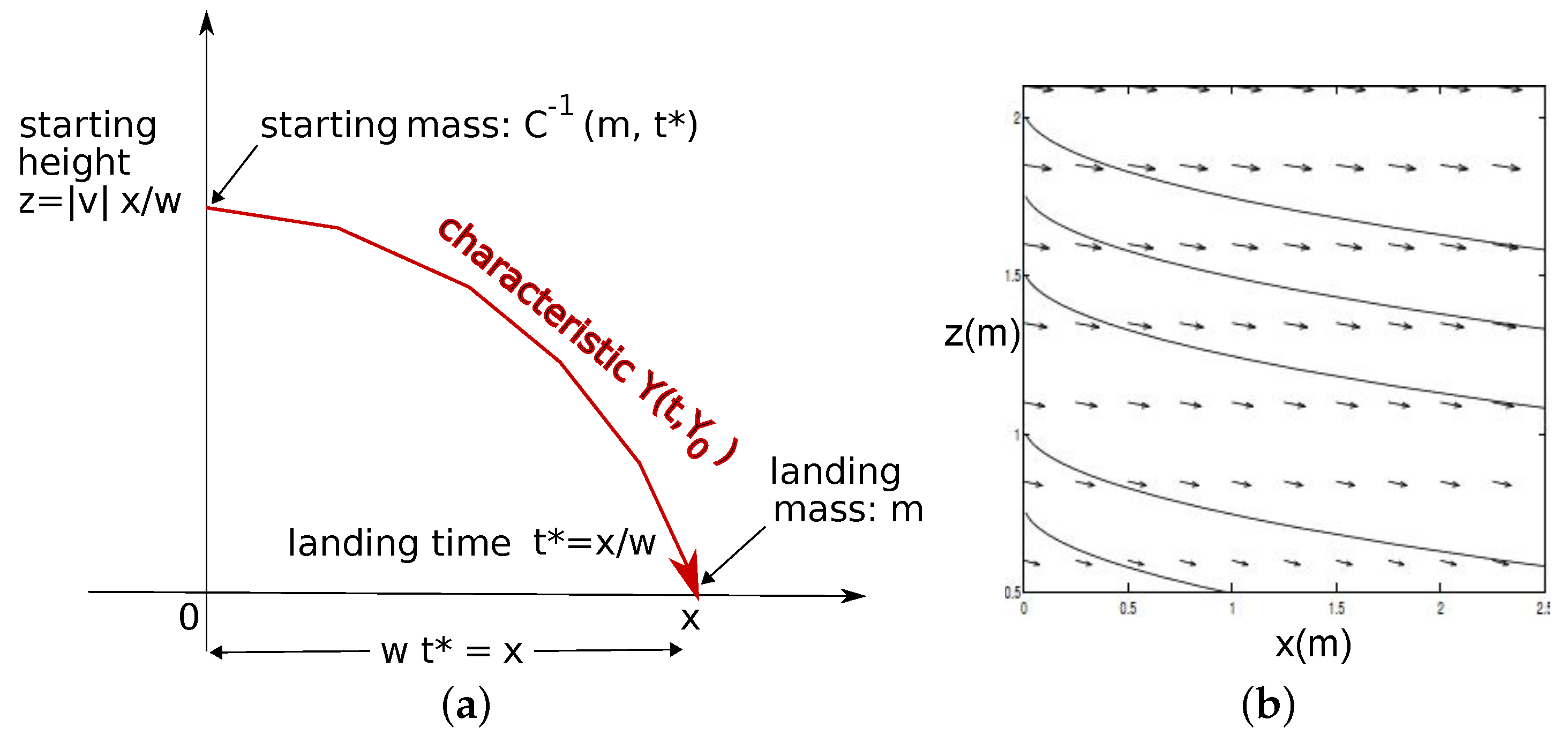
A schematic for the use of the method of characteristics, in case of constant wind and constant terminal falling velocity, is shown in Figure 2a.
2.3. From Landed Firebrands to the Spotting Distribution
The “landed brands” are those that reach the canopy at height (where we assume that they fall straight to the ground—meaning we neglect within-stand winds and resettling, although both effects can be considered [49]). We can track these explicitly according to the solution Equation (19) of the impulse-release IBVP for the transport Model (5) described earlier in this Section. We recall from the introduction to Section 2 the distribution keeping track of all brands that have landed before time t, namely the landing distribution
and recall that the limit as the asymptotic landing distribution
To determine the spotting distribution, we must first integrate the asymptotic landing distribution appropriately, to obtain the landed masses in kilograms. Employing the inverse combustion operator and the landing time , the mass in kilograms at location x is given by
Finally we can determine the spotting distribution in terms of the latter, by employing the ignition operator E, which we recall maps mass in kilograms to values in , as follows:
Our use of the spotting distribution is similar to the Green’s-function approach that is used in the study of linear partial differential equations [50]. The Green’s function describes the evolution of an impulse release, and the full solution to a PDE can be found by integrating the Green’s function against initial and boundary conditions.
In the examples in the next Section, we show some illustrative but simple spotting distributions. We have seen that the spotting distribution depends on various physical submodels for firebrand launching, flight, burning, landing and ignition. In the Appendix, we provide a detailed review of the most commonly used submodels, which we summarize in Table A1. Each combination of these submodels leads to a reasonable spotting distribution. This gives more than 500 cases, which we cannot cover in this paper. Hence, in the next Section, we focus on some easy to understand examples, which we identify by their corresponding model number as used in Table A1. We hope that the present work will generate interest, especially in the experimental community, in order to determine the most physically plausible spotting distributions for a variety of important spread scenarios.
3. Examples of the Spotting Distribution
3.1. Case (W1,V1): Constant Wind and Terminal Velocity
(Case (W1,V1) in Table A1). As explained in the Appendix, wind-tunnel experiments show that firebrands quickly take on their terminal speed and configuration [9,51]. Of course, the firebrands are combusting, so the speed and geometric properties will evolve with time. As a first approximation, and in the interest of analytical tractability, we will assume firebrands fall with constant velocity and constant wind . All combustion models studied here (F0–F6) have a combustion rate that is independent of the mass. Hence here and throughout we assume .
The landing time will be important in what follows. To present a concrete example, if , , then the landing time for firebrands launched initially at to arrive at is .
As a starting point, fix a point in the quarter plane , and assign a time . If , then the firebrands which started at 0 have not yet reached location x, so we can determine the firebrand density from the initial condition for p. However, if , then we must determine the firebrand density by integrating backwards along characteristics to the boundary at . The latter requires solving Equations (11) and (12) with negative signs in front of the terms on the RHS. It is clear, then, that the firebrand density, provided N firebrands are released above a canopy of height H, is given by
where is the vertical launch distribution, and is the inverse combustion operator. A schematic of this solution is shown in Figure 2a. We remind the reader that at we have for , from our initial condition for an impulse release, so we find for . Recalling that the distribution of landed brands is given by for , so we find:
where represents the Heaviside, or unit-step function, defined by for , and for .
Taking the limit as in Equation (26), we obtain the asymptotic landing distribution ,
This equation maps the launching distribution to the asymptotic landing distribution , as depicted on the right of Figure 1. We will compute some explicit examples in Section 3.6.
We impose the assumption, that if:
This is to assure that we do not obtain any negative mass density.
We see that the asymptotic landing distribution in Equation (28) is simply the number of firebrands released N, multiplied by the vertical launch distribution with its arguments shifted. We employ this remarkably simple result in the next subsections, for important vertically-varying horizontal wind profiles.
3.2. Case (W3,V1): Power-Law for Wind, Constant Terminal Velocity
In the previous subsection we explored the case where and are constants, corresponding to constant wind and constant falling terminal velocity. We also made no discussion of the canopy; the approximation that the canopy height , can be useful in describing long-distance spotting events, as on this spatial scale the canopy height is negligible. Increasing slightly our model complexity, in this subsection we consider a ‘power-law’ wind profile, first employed in the context of spotting by Albini [1]. We model the horizontal windspeed as a function of height z above the canopy by
where H is the canopy height, is the windspeed at the canopy’s base, and . We are interested solely in values of . Further, we will not consider resettling or within-canopy winds, so we assume once a firebrand has reached , it drops straight downward, and is immediately capable of igniting a new fire. We will continue to assume .
With all this said, the spatial characteristics read:
The solution to the first equation, given an initial condition , is , which we then use to solve the equation for x. Notice that since , the heights z are decreasing with time. The Equation (31) for x becomes:
Integrating both sides with respect to t, we obtain:
Now consider a firebrand which reaches the canopy at . We wish to determine the landing time which it took for the firebrand to travel from at time to the top of the canopy at . As in the preceding subsection, we will run the characteristics in reverse. To do this, we choose , , and , and insert these values into:
We obtain:
The reader will notice that in the case where , Equation (37) reduces to , which is consistent with the constant w, constant v case in Section 3.1.
We find the exact solution p of our impulse IBVP for the transport and combustion process:
where
so that the bounds on x appearing in Equation (38) can be written in explicit terms, through the following expression:
We can interpret the latter integral in Equation (41) as the location of the leading edge of the expanding firebrand distribution , since for , but when .
In particular, from Equation (41) we see that . So we can argue similar to the preceding subsection, arriving at the asymptotic landing distribution (which appears very similar to Equation (28)):
but here the landing time is given by Equation (37). Again, as shown in Figure 1 (b), we obtain a map from launching to landing . Notice that we set if (i.e., we allow only nonnegative masses).
3.3. Case (W2,V1): Logarithmic Profile for w, Constant Vertical Velocity
In this subsection, we again assume a constant vertical velocity , and we introduce the logarithmic horizontal wind profile (first employed by Albini in spot fire modelling [1]):
where , is the friction velocity, κ is von Karman’s constant, is the zero-datum displacement, where H is the canopy height and d is the distance above the canopy where horizontal winds begin [49]. We will approximate .
As in the preceding subsections, we may determine the landing time . After some work (see [29] for details), we arrive at an implicit expression for the landing time:
For given values of the parameters we can then use a numerical method, like Newton’s iterative root-finding method, to compute the landing time as a function of x to any desired precision, since we cannot obtain an explicit expression for the landing time. Because the landing time must be increasing with x by uniqueness of firebrand trajectories, with some more work we obtain once more a very similar expression for the the asymptotic landing distribution,
though the formula is slightly less attractice since must be solved implicitly from Equation (44).
3.4. The Spotting Distribution Determined from
The uniqueness of firebrand trajectories for the constant wind, power law and logarithmic wind profiles, and the assumption that the ignition probability depends only on the landed mass, will allow us to use the asymptotic landing distributions obtained in the previous section, to obtain the spotting distribution . Recall our Formula (23) for the spotting distribution; having computed several asymptotic landing distributions, we now have several examples of the spotting distribution. Our assumption that the continuous ignition operator depends only on the landed mass implies that the spotting distribution , which characterizes the probability of a spotfire igniting due to an impulse release from , is given by:
An explicit example for constant wind is given in Section 3.6.
We can extend this concept to firebrands released at location , at time , to determine:
The Formula (47) describes the kernel for a firebrand release at , at time . Notice that our expression is very general, in that we are free to employ a variety of ignition or combustion models, through inclusion of specific functional forms for or C respectively.
3.5. Case (W1,V1, F0, L3, I3): A Family of Simple Spotting Kernels
Let us consider the threshold ignition law (I3) presented in the Appendix, in the case where (see Equation (A35)). Then any firebrand landing on a location which is not burning, will instantly generate a fire. We again have constant w and v, and further we will suppose that no mass is lost during transport corresponding to the constant burning law with zero rate of combustion (the transport process being assumed very rapid).
Let’s assume that the firebrand vertical launching distribution satisfies the assumption (L3), so that
This says the lofting heights z are independent of the masses m. This may occur, for example, in the case of well-mixed line thermals. We can choose the mass distribution in accordance with experiments such as in the experiments by Manzello [5], or out of mathematical curiosity we could consider any other probability distribution. What is most important is to assume that is not exponentially bounded, in order to obtain a fat-tailed kernel. For example, one could assume:
for . This kernel is of particular interest here, since it decays sub-exponentially, and has been shown in integro-difference models [26] to give rise to accelerating propagation of the corresponding solution in space [26]. Physically this could correspond to extreme spotting conditions like in the presence of fire whirls.
From Equation (46), with the form Equation (49) appearing in the landed mass distribution , we find that for a release of N firebrands the landed distribution of masses at location x is:
where is the total landed mass at x, namely
Since we are assuming instant ignition, the spotting distribution is the same as the landed mass distribution. Referring to Equation (50), we can then write the spotting kernel in this case:
3.6. Applications: Examples of the Spotting Distribution
In this subsection we show some explicit examples for the landed mass and for the spotting distribution. First we consider an explicit version for the cases (L3, G1, W1, V1, F0, I2), which is a special case of case (W1, V1) that was studied in Section 3.1. We consider
According to Formula (28) we have a landing distribution of
Substituting the explicit forms from Equations (58)–(62) into the landing distribution, we get an explicit formula for :
The condition implies that
and
To obtain the total landed mass, we multiply with m and integrate from 0 to :
Now we use the integral
and we find and explicit formula for the landed mass
To obtain the spotting distribution, we need an ignition law. Here we use the piecewise linear ignition function with lower ignition threshold and we obtain
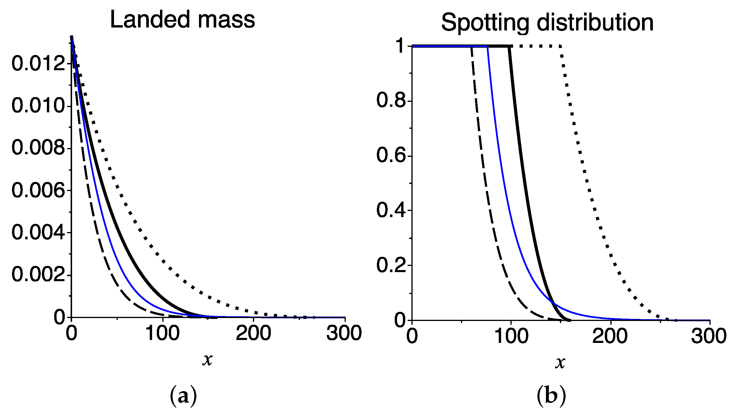
with given by Equation (70). Hence we find an explicit formula for the spotting distribution. As examples we chose the parameters as in Table 1 and we plot the landed mass and the spotting distributions for these cases in Figure 3.
The parameters in Table 1 have been chosen to model realistic physical scenarios, at the lower limit where spotting might begin to have an impact. The windspeed w of two metres per second is on the low end of observed values [3]. Terminal speed of one metre per second is also low, but on the same order of magnitude as firebrands with diameter, mass and length as described in Manzello’s study. The upper and lower bounds on the mass, measured in kilograms, correspond to the values found in Manzello’s combustion experiments [5]. The rate of combustion, chosen between 0.03 and 0.05 g per second, results in flaming burnout in under two minutes. Choosing 1000 firebrands, corresponds to combustion of about ten trees—a moderate estimate for the width of our front. The decay rates λ were chosen so that firebrand launching would drop off appreciably beyond several hundred metres. Finally the parameter a is a normalization constant for our mass distribution.
Next we consider the effect of changing combustion model, choosing instead our modified version of Tarifa’s model (F2), while keeping all other parameters fixed (see Table 1). It is thus important to reconsider the inverse combustion operator. According to the model (F2), we have
since this is the initial mass, which travelled through the air after launching during a time of . We can start with Equation (65) and replace the term by . Then the landed mass is computed to be
and the spotting distribution is again explicitly given by Equation (71). As an example we use parameters as in Table 1 and plot the landed mass and the spotting distribution as thin blue lines in Figure 3. Notice that the inverse combustion operator in Equation (72) is always positive for all . Hence in this case we have no maximum spotting range and = ∞, even though it is effectively zero beyond 200 m.
It is important to determine the minimum spatial extent of the spotting distribution required for spotting to be important. Below this extent, the main fire will outrun spot fires before they can develop into a separate front. As a specific example, Alexander has estimated such an effective distance for crown fires in North America to be approximately 300 m (in the most extreme ignition conditions [3]). In Figure 3 we consider Alexander’s crown fire situation. In comparing the Tarifa-case with the dotted curve (base case with slower burning), both distributions extend at least approximately to the 300 m cutoff—though in the Tarifa-case the distribution is essentially zero there. We further note that, while not shown, just halving the combustion rate in the base case pushes the distribution past the 300 m mark. By changing the combustion model or parameters, we obtain very different outcomes for the importance of spotting.
4. Discussion
4.1. Usage of the Spotting Distribution
One of our primary motives in determining the spotting distribution, is to employ the latter as a redistribution kernel in fire spread models. For example, the model in [35] uses an indicator function approach to describe the interface between burned and unburned regions. They include spotting in the form of a log-normal distribution, but other spotting distributions, such as computed here, could be included as well.
A somewhat different approach was taken in [29,30], where an integro-PDE equation approach was used to model the probability of fire at a certain location. The time evolution of the likelihood to observe a fire a time t at location x is given by the integro-PDE
where is the spotting distribution, describes combustion, denotes the heat loss term and the diffusion describes local fire spread. This model was used in [30] to investigate invading fire fronts and their asymptotic invasion speeds. For example, we could there show that spotting is able to increase the fire invasion speed. A model of the above type is quite versatile and it can include various spotting distributions as well as different combustion and fuel dynamics.
A more standard approach starts from conservation laws for physical quantities like energy of chemical species, leading to coupled reaction-diffusion systems for temperature and mass evolution [31,52,53] and knowledge of the spotting distribution might be a useful addition to these models.
Changing gears from our discussion of the “spread problem”, knowledge of the spotting distribution is also important for the “breaching problem”—of great practical importance for wildfire management, but poorly understood. For example, suppose a crowning forest fire reaches a wide river. On the opposite side is a continuous stretch of dense coniferous forest. The likelihood of a spot fire occurring on the non-burning side of the river equals the integral of the spotting distribution along the opposing side of the river. It gives a direct quantitative measurement for fire risk beyond fuel breaks. A similar problem arises at the wildland-urban interface and the spotting distribution can tell us how far the spotting is likely to reach.
4.2. Measurements of Spotting Distributions
The primary challenge for the spotting experimentalist is the paucity of quantitative observations from real fires. The landing fire brands could be visualized by visual recording or infrared recording. In the paper “Monitoring Insect Dispersal”, by J.L. Osborne et al. in the collection [27], the authors discuss “vertically looking radar” (VLR). Such radar has been used to study insect dispersal, and consists of a series of gates capable of monitoring the skies from 100 m to a kilometre above ground. In addition, the VLR system is capable of determining flying mass, direction and magnitude of the velocity vector of a flying brand. One could imagine field experiments where such instrumentation is employed, in order to count how many, to which height and with what mass are the firebrands being released.
In field situations, the ignition probability can be estimated by the number of spot fires which result per unit of landed firebrand mass, or ideally extrapolated from laboratory experiments. Satelite data, or other forms of radar collection could be of use here as well; while individual spotting events may only be observable through the appearance of a new fire, if we had detailed spotting information for a particular fire situation, such information could help inform the likelihood of long-distance dispersal.
There are some field experiments, in particular from Australia’s Project Vesta [54,55], where attempts have been made to directly measure the spotting distribution. In particular, in a series of experimental fires, firebrand distributions were measured by catching brands on plastic sheets. The goal was to validate earlier firebrand modelling employing the CSIRO wind tunnel by Ellis [9], though the results were mostly qualitative and the need for model improvement was a primary finding.
In controlled lab experiments, several trees could be alighted in a wind stream and all landing embers can be first put out, then counted and weighed, as has been done in experiments by Manzello [44,45]. Both of these approaches (field and lab) give us the landing distribution . To get the spotting distribution we need a second ingredient, which is the probability of ignition . Several lab experiments have been done already, where burning material is thrown into various fuel beds and the ignition probability has been measured using regression analysis in quite some depth ([46,47]). In the very hetereogeneous natural spotting environment, understanding the variability in spotting ignition probabilities over space and time is very important.
We believe that many of this data is already available in various fire management and research centers, but, to our knowledge, they have not been systematically examined to estimate a spotting distribution. Promising data are available for example for the 1961 Basin Fire in the Sierra National Forest (USA) [56], the 1994 South Canyon Fire in Colorado [57], the 1994 Butte City Fire in Idaho [58] and the Oakland/Berkeley Hills Fire [59], which in particular was described in the review paper by Koo et al. [12]. We leave a detailed exploration of these data to future research and we write this paper in the hope of generating increased interest in better quantifying the lesser known model components.
We have seen that the derivation of specific spotting distributions depends on many physical details, which we outline in the Appendix. However, direct measurement might enable us to skip the detailed physical modelling and rather use an empirically measured spotting distribution.
4.3. Future Studies
The key idea behind the spotting distribution is a separation of time scales for the relevant processes, namely the fast wind-distribution of firebrands versus the relatively slow crawling combustion of the main front. In real wildfires, the total flight time of burning material is of the order of seconds to minutes, while we may assume that the overall fire front progression is of the order of minutes or hours. The maximum possible flight time of firebrands has been established through wind-tunnel experiments, which confirm that combustion of firebrands results in extinction after at most several minutes, and flaming combustion even prior to that, though there is the possibility for re-flaming if travel is fast enough (e.g., [5,9,31]). Ignition is highly dependent on firebrand state upon landing (e.g., flaming vs. glowing). For forest fires, the required separation of timescales between spotting and local spread is valid—wind transport is much more rapid. For grass fires, however, the time scale of local spread and spotting is comparable and our scaling argument is invalid for grassfires.
We only consider horizontal winds perpendicular to the main fire front. However, dispersal of firebrands happens in all directions, often leading to a “V”-shaped spread downwind—similar to the wake left by a boat travelling through water. In our case, any spread parallel to the front will not change the front’s shape. However, increased travel times due to horizontal movement parallel to the front’s axis may lead to decreased support for the downwind landing distribution, due to earlier burnout. Further, there may be a greater net accumulation of firebrands than is described in our distributions, due to cross-wind contributions from launches further down the front. The latter point is less concerning, since there is already uncertainty in the number N of firebrands launched. Since our idealized distributions will be translation-invariant parallel to the front, extra accumulation could be accounted for by increasing N.
From a mathematical perspective, integro-differential equations, which employ redistribution kernels to describe long-distance dispersal, such as Equation (74), have become of much greater interest of late. There is considerable overlap with research on plant seed dispersal [26,28] and we expect that analysis methods that are used in seed dispersal to become useful for fire spotting as well. Employing our spotting distribution as such a redistribution kernel, we hope to be able to provide more complete answers to the questions posed in Section 1.3. Including topography, spatial variation in fuel and weather leads to heterogeneous and nonlinear mathematical models, which would be further complicated—but made more realistic—by adding an additional spatial dimension.
Many avenues of research are opened by considering the analysis of such models, since such models are mathematically complex and at the forefront of current applied analysis and numerical modelling research. Hence another way our models could be improved is a better understanding of the analytical aspects of nonlocal models in heterogeneous media, which is another avenue of research underway by the authors and others [60].
Acknowledgments
This work resulted from a MITACS (Mathematics of Information Technology and Complex Systems) Full Project on Forest Fire Modelling. The authors are grateful for feedback and support through the researchers involved in this MITACS project. Details of this work were discussed during Journal Club meetings at the University of Alberta, and we are grateful for the lively interest and feedback from the Journal Club participants. Parts of J.M.’s work was supported by the PIMS (Pacific Institute for Mathematical Sciences) International Graduate Student Training Centre, two MITACS summer internships, and part of this work has been carried out in the framework of the project NONLOCAL (ANR-14-CE25-0013), funded by the French National Research Agency (ANR). T.H. is grateful to support through NSERC (Natural Sciences and Engineering Research Council of Canada).
Author Contributions
The models and results of this paper are part of Jonathan Martin’s PhD thesis [29] under supervision of Thomas Hillen. The model derivation and analysis, as well as the writing of the manuscript has been done in equal parts. The extensive appendix was developed by Jonathan Martin.
Conflicts of Interest
The authors declare no conflict of interest.
Appendix. Ember Release, Burning, Flying and Fuel Ignition
In this Appendix we will discuss the modelling of physical subprocesses that are involved in the spotting problem. We will review the extensive literature in this area, and derive mathematical models for the firebrand mass distribution, plume models and the vertical launch distribution, firebrand combustion and temperature, vertical and horizontal transport speeds, and ignition probabilities. We summarize all models and their references in Table A1.
Appendix A.1. The Launching Distribution
The greatest challenge in modelling spotting is to determine how many firebrands, distributed according to their various characteristics, are both generated and subsequently launched into the atmosphere. The latter process takes place in the fire plume, which is a high-velocity, buoyancy-driven flow induced by the combustion at the surface [61]. The plume of a wildland fire is often called its convection column [32]. Any fire plume is more turbulent than laminar, and our knowledge about plumes is mostly experimental [61]. There is a complicated interaction between the atmosphere and the fire, hereafter referred to as fire-atmosphere interactions, which has been extensively studied from experiments, and physical modelling [1,2,17,18,22,23,24,31,62,63,64,65,66,67].
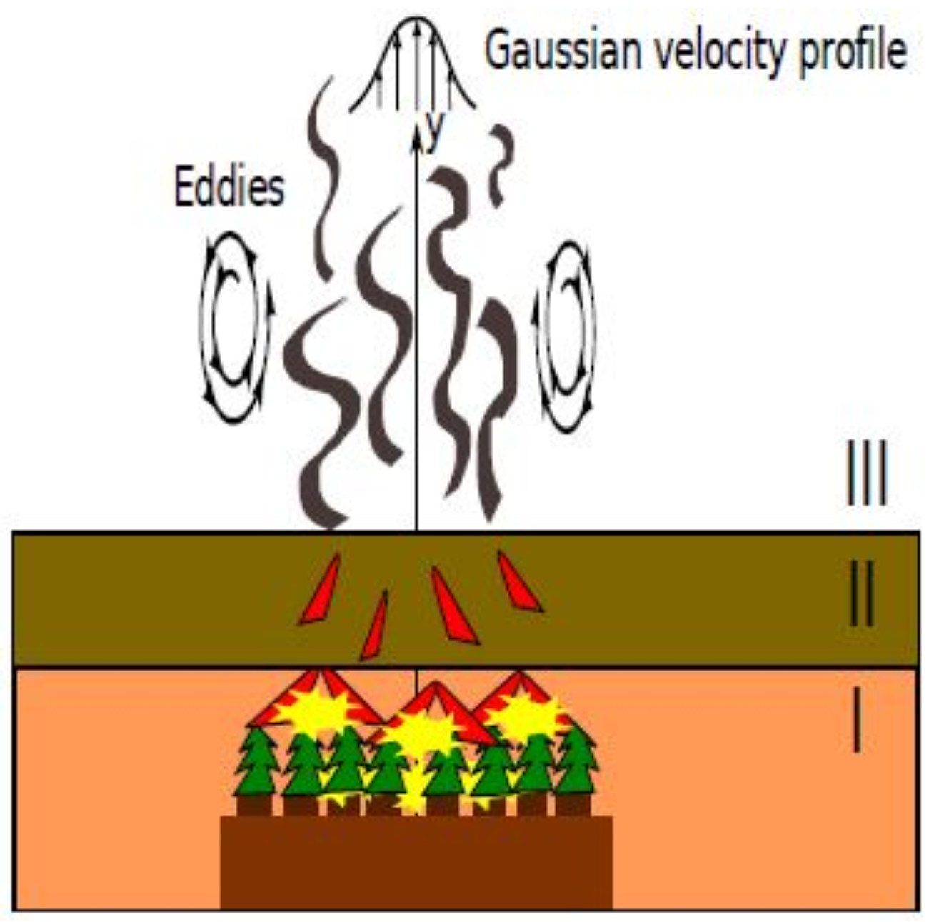
The most widely used fire plume model in spotfire modelling is the model developed by Baum and McCaffery [18,21], as used for example in [1,7,13,19,20,22,67]. The model consists of three burning regions, illustrated in Figure A1. Our discussion here closely follows that of the book [61] and the paper [22]. Region I lies at the base, and is the continuous burning region. Here the flow is pulsating and unsteady. Region II is an intermittent zone, in which flame patches break off from the below-anchored flame, while at the top of Region II all combustion ceases. Finally we have region III, the non-combusting plume, where we assume that the time-averaged upward velocity and temperature drop off radially in a Gaussian manner.

| Process | Number, Description | Reference |
|---|---|---|
| launching | L1, Unique launching height | [1,21,22]. |
| L2 , Normally distributed | New. | |
| L3, Heights and masses independent: | ||
| New. | ||
| launched mass | G1, Power law | New; [44] |
| G2, Slash burning | [32]. | |
| Wind transport | W1, Constant horizontal wind | New. |
| w | W2, Logarithmic wind profile | [1,15]. |
| W3, Power-law wind profile | [1,13]. | |
| Terminal vertical | V1, Constant v | [9,68]. |
| velocity v. | V2, Experiments on | |
| cylindrical firebrands. | [16]. | |
| Combustion models | F0, Constant burn rate | New. |
| f | F1, Tarifa’s model | [1] |
| F2, Simplified Tarifa’s model | New. | |
| F3, Negligible combustion | New. | |
| F4, Fernandez-Pello model | [69]. | |
| F5, Refinements to | ||
| Fernandez-Pello model | [22,70]. | |
| F6, Albini’s line | ||
| thermal model | [3]. | |
| Ignition probability | I1, Piecewise linear | [32,46,47]. |
| I2, Heaviside step function | New. | |
| I3, Smoothed step function | New. | |
| Temperature | T1, Newton’s Law of Cooling, | |
| T2, Stefan-Boltzmann law | [22]. |
Figure A1.
Sketch of the Baum and McCaffery plume. Region I is the continuous (canopy) burning region. Region II is a transition zone over which the plume velocity is constant. The buoyant upward motion in region III is reinforced by large ambient eddies, which cause entrainment of air into the plume.

The relevant parameters are height z, plume velocity , and temperature T. These are made dimensionless by the scaling where:
The parameters appearing in Equation (A1) are the heat release rate Q, the density of air kg·m, kg·K is the specific heat capacity of air at constant pressure, is the temperature of the ambient air, and g is the gravitational constant.
The analysis in [71] then leads us to the mean plume-centerline velocity and temperature as a function of the rescaled height :
For a given height z in the plume region there is associated a unique mass , such that this mass attains terminal velocity exactly at height z. In other words, the drag induced by the upward plume velocity is balanced by the weight of the mass at this height.
In the idealized case of a spherical particle, we have a direct connection between the cross-sectional area A, the diameter d, the drag coefficient and the density . Employing the relation Equation (A2), we obtain the unique lofting height:
Employing Equation (A1) in the latter equation, we can re-write the lofting height as:
We will introduce a constant which absorbs all the constants in Equation (A4), and re-write the Equation:
Recent work suggests that the fire-atmosphere interaction results in distinctly non-Gaussian distributions [22]. In the physically realistic computer simulations of grass fire plumes of [22], which employs a Large Eddy Simulator to model the atmospheric winds, the time-averaged velocity profiles are not observed to be Gaussian and the Baum and McCaffery plume model needs to be extended.
Based on these observations, we study three launching models:
Model L1. We assume that each firebrand of mass m is lofted to a unique height , as for example in Equation (A5). We can then define
where is a given mass distribution, and δ represents the Dirac delta functional.
Model L2. Instead of assuming that each mass is lofted to a unique height, we might instead suppose that it is launched randomly about the standard lofting height . For example, if heights are normally distributed about the lofting height , we can write , a one-sided normal distribution where has mean and variance σ, with
where the constant A is chosen so that the distribution is normalized. We allow values of z to lie in , where H is the canopy height and is the maximum lofting height predicted by the Baum and McCaffery plume.
Model L3. Finally, we consider the case where the launching heights z, and masses m, are independent of each other, so we can write
where is a probability distribution which describes how firebrands are distributed with height z, and is the mass distribution.
A similar sort of model was employed by Albini in the context of firebrand transport by line thermals [13], where is a uniform distribution .
Appendix A.2. Distribution of Launched Masses
A recent series of studies by Manzello and colleagues [5,44,45] investigated firebrands emitted from the controlled burning of either pine or fir trees. In the Manzello experiments, trees both 2.6 m and 5.2 m tall were investigated. For each tree, more than 70 firebrands were collected. These were all cylindrical in shape. The average firebrand length and diameter for the 2.6 m class was 40 mm in length and 3 mm in diameter, while for the 5.2 m class the average was 53 mm in length and 4 mm in diameter. The most recent of the experiments, on Korean pine [44], confirmed that the distribution was approximately the same. The total number of firebrands collected numbered almost 1000.
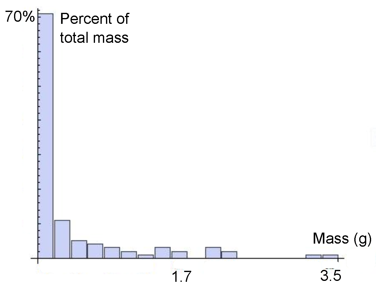
With respect to mass, all three of Manzello’s studies indicate that between 60 and 80 percent of the firebrands have masses less than 0.1 g. Further, for both pine and fir taller trees produce larger firebrands, with the largest found at about 5 g. In addition, between 58 and 65 percent of the firebrand mass is needles, which are insignificant in long-range spotting, but may be effective at igniting local fuel only in short-range spotting [46]. We remove the needles from Manzello’s mass distribution, to obtain an ‘effective mass’ distribution.
Model G1: Regression analysis on Manzello’s data. In order to determine a functional form for the effective mass distribution, we reproduced the histograms from [44,45], an example of which is shown in Figure A2. Between 60 to 70 percent of the mass is needles which are negligible for long-range spotting. Hence we first removed the needles lying in the 0.1 g mass class, to obtain an effective firebrand distribution. We use non-linear regression of the functional form:
where , corresponding to the maximum firebrand mass. Regression analysis gives , and , which gave a better fit than an exponential form.
Figure A2.
The mass distribution for the 5.2 m Douglas fir firebrands plotted as histogram from the data from [5]. The histograms for the other taller specimens for each species studied are similar. Along the x-axis we plot firebrand mass in grams.
Figure A2.
The mass distribution for the 5.2 m Douglas fir firebrands plotted as histogram from the data from [5]. The histograms for the other taller specimens for each species studied are similar. Along the x-axis we plot firebrand mass in grams.

Model G2: Models obtained from burning slash. Another firebrand distribution was suggested in [32], which relates the possible radius r of a firebrand to the mass consumption rate f, in the form:
where and σ were parameters determined by regression analysis, and α represents the number of firebrands generated per unit mass. If we assume a relationship of the form , where ρ is the density and is the firebrand volume, then from Equation (A11) we find the mass density:
where δ denotes the Dirac delta distribution.
From the experiments of Manzello described in this chapter, it was found that approximately one percent of the total mass lost during combustion appeared as firebrands. This could inform our parameter α, and in turn determine the total mass and total number of firebrands released when a given number of trees begin to spot.
Appendix A.3. The Atmospheric Boundary Layer
The atmospheric boundary layer (ABM) is the lowest portion of the atmosphere, extending on average about one kilometre, and ranging up to at most about three kilometres above the Earth’s surface [72]. It consists of a number of distinct sublayers, and it is of utmost importance since the ABM is where firebrand transport occurs. At the bottom is the laminar sublayer, which has a thickness of only a few millimetres. This is a region where high viscosity, induced by the “roughness” of the surface, results in molecular diffusion being the basis for transport of momentum and heat [73]. Above the laminar layer is a transition region, leading into the Prandtl layer, in which turbulent convective motion is the dominant transport process [73]. The lower boundary of the Prandtl layer is called the roughness height . At the top of the ABM is the Ekman layer, throughout which the effects of turbulent convection lessen with height, decreasing to zero near the top of the Ekman layer [73].
Firebrands are transported by convection, and hence are subject to the turbulent fluctuations in wind velocity present in the ABM. Turbulence is a dissipative process which converts kinetic energy in a fluid into heat energy, and it is essentially three-dimensional and rotational [74].
Turbulent eddies, which may be envisioned as large sheets of wind rolling over one another, exist on length scales from m to m. The largest eddies can therefore extend up to the height of the ABM [74]. In the case of a fire’s convection column, the eddies swirling parallel to the column result in the entrainment of ambient air into the column [22].
Because of the inherent variability in the transport process, we introduce the standard Reynolds decomposition for the velocity components [74]. This means we decompose the horizontal velocity w into a slowly-varying mean component and a rapidly-varying component , so that:
In general the mean windspeed increases with height, though exactly how this happens is effected by surface roughness and variable topography, to say nothing of the fire-ABM interactions. In our transport model we will be interested in the time-mean behavior of the stochastic flight process, so we will focus exclusively on the mean velocity . We drop the bar in what follows for notational simplicity.
Model W1: Constant horizontal wind. The simplest assumption for the windspeed w is that it does not vary with height z, so that
Model W2: Logarithmic horizontal wind. Another commonly used wind model is the logarithmic profile, introduced in the context of spotting first by Albini [1]:
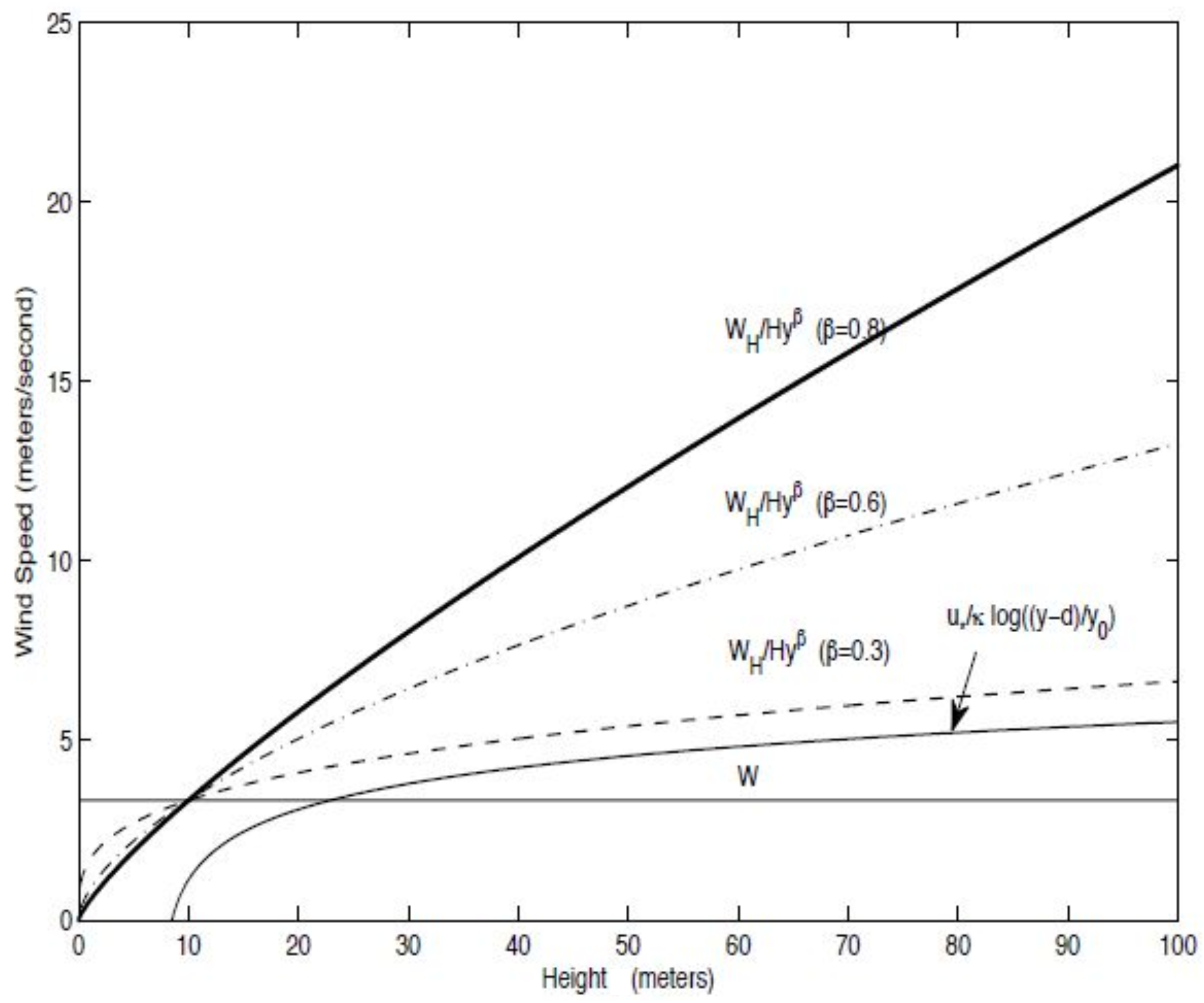
Appearing on the right hand side of Equation (A15) is the von Karman constant , the roughness height , the zero-datum displacement d, and the friction velocity . The friction velocity is generally defined by , where T is the time-mean flux of tangential momentum towards the surface, borne by turbulence outside the lower ABM and by viscosity within it [15]. Typical values for in a strongly upward-convective atmosphere are around m/s, while for a roll-dominated atmosphere m/s [24]. The roughness height corresponds to the lower boundary of the Prandtl layer. At the upper end examples include m for dense forest or shrubs, m for low crops or bushes, and flat grassland has m. When there is significant roughness or dense forests, the zero-datum displacement d is employed in Equation (A15) to offset the height at which the windspeed aloft vanishes. The value of d is usually about 2/3 the average height of the obstacles. We show velocity versus height for three different cases in Figure A3.
Figure A3.
A comparison of the wind profiles discussed in this Section. Shown are three power-law models for different values of the parameter β, together with a logarithmic wind profile and a constant wind profile. We have chosen m/s, and the canopy height to be 10 m.
Figure A3.
A comparison of the wind profiles discussed in this Section. Shown are three power-law models for different values of the parameter β, together with a logarithmic wind profile and a constant wind profile. We have chosen m/s, and the canopy height to be 10 m.

Model W3: Power-law wind profile. A third wind model was also first introduced in the context of spotting by Albini [1]. It assumes a power-law profile for the horizontal velocity versus height,
where H is the canopy height, is the windspeed at the canopy’s base, and . In Albini’s work, he chose the constant [13]. Model (A16) is a better approximation to the windflow when it is over terrain which is not covered by tall vegetation. Further, this model may be seen as an approximation to the logarithmic profile, and is consistent with the constant-wind model (to see this, set in Equation (A16)).
A comparison of our three functional forms is presented in Figure A3.
Appendix A.4. Drag, Gravity and Terminal Velocity
In order to accurately model the falling of firebrands in the atmosphere, it is important to model the drag experienced by the firebrand. Often, the drag is proportional to the object’s speed, or speed squared, depending on the Reynolds number of the flow. For firebrands, it is more accurate to model drag as proportional to the speed squared, since we have a relatively high Reynolds number flow [22].
Let us denote the drag force by D. Then the speed-squared assumption is generally written as:
where refers to the mass density of the ambient fluid, and the object is assumed to have constant cross-sectional area A. The parameter appearing in Equation (A17) is called the drag coefficient. This is a dimensionless number, with values typically ranging between 0.001 and 2, assumed to vary with shape. This constant is typically determined by experiment.
Newton’s Second Law then provides us with an expression for the terminal velocity. If we focus on the vertical direction, the balancing of the drag force D with the weight W implies:
Model V1: Constant terminal velocity. The simplest assumption (V1) is to assume the terminal velocity does not change during transport.
Model V2: Experimentally determined model. Experimental analysis on the Aerospace Corporation’s experiments, appearing in [16], revealed that for the cylindrical firebrands in the study the mass is related to the terminal velocity according to:
Appendix A.5. Firebrand Combustion
Several combustion models have been proposed in the literature, and the interested reader is invited to peruse the review in [7]. They are usually modeled as continuous-time processes, so we will present functional forms for the density, effective radius, or simply the mass as functions of time.
Suppose the mass is the unique solution of the initial value problem
where f is the rate of combustion. We introduce the combustion operator C as the unique solution
In our spotting problem, we need to compute backwards. If a fire brand of mass m lands, then we like to know its initial mass . Hence we define the inverse combustion operator , which is the unique solution to the initial value problem at time . Before continuing, it is important to note that the combustion process does not continue past the point where the firebrands have masses less than or equal to zero. Hence the combustion operator is only defined up to the burnout time , and similarly for its inverse.
Model F0: Constant burning rate. Suppose the burning rate is a constant , then we have , and . The inverse satisfies for .
Model F1: Tarifa’s original experiments and models. The first experiments on the density and shape changes in combusting firebrands were carried out by Tarifa and collaborators at the Aerospace Corporation [1]. This data was fit by regression analysis obtained from windtunnel experiments, where both spherical and cylindrical firebrands were examined under a variety of ambient windspeeds.
Suppose represents the density of a firebrand at time t, and is the initial density. Then Tarifa found the density varied as:
where the constant was determined from regression analysis.
Models F2: Caricature of Tarifa’s model. We employ an analogue of Tarifa’s density evolution for the mass , namely
Model F3: Constant mass. If we take case F2 to its extreme, sending , we get
Model F4: Tse and Fernandez-Pello’s improvements. Tse and Fernandez-Pello revisited Tarifa’s data set [75], and determined the model which best fit the data for the effective radius evolution is:
Clearly the latter is only defined while , which implies a finite burnout time. Here the parameter χ depends on the wood species and moisture content of the firebrand, and β is described below in the derivation of Equation (A31). Based on Tarifa’s data, the parameter gave the best fit [69].
To determine the mass , we first employ the simple relation:
where is the volume of the firebrand, and hence dependent on the radius .
As a simple example, suppose the firebrand is approximately spherical, so that . Then we combine Equations (A24) and (A26), so that the mass evolution Equation (A27) is given by
Taking for example cedar wood as representative of forest fuel, as did the authors in [22], the initial density of the firebrands would be 513 , while in the experiments of Manzello [44] he found radii ranging from one half to five centimetres.
Another important result following the analysis in [69], is that one can reasonably approximate extinction of the firebrand to occur once:
where is a critical mass ratio which depends on the wood species. Beyond this point all that remains is non-flaming char, whose temperature then decreases according to Equation (A42) described in the next subsection. From regression analysis in [69], we find for maple and pine.
Model F5: Including more physical realism. Another model has been derived in [22], and is based in part on experimental fitting of data by Tse and Fernandez-Pello [69]. It is based on Nusselt’s physically-motivated combustion theory, known as ‘shrinking drop theory’ [22,70]. We include a discussion of the model here because, as we will see later, the firebrand’s burning temperature may influence its flight path significantly [22]. In Nusselt’s combustion theory, the firebrand’s surface is assumed to be held at constant temperature, maintaining its geometrical shape while a pyrolysis wave propagates inward. One employs the so-called Frossling relation, in which we define the effective mass diameter , and an experimental constant β, such that:
The constant β, introduced earlier in Equations (A26) and (A28), is determined physically from the equation:
where on the right hand side we have the Reynolds number , and the Schmidt number , and an experimentally determined constant . The Reynolds number , where is the firebrand’s speed relative to the surrounding air, r is the firebrand radius, and is the kinematic viscosity of the surrounding air [22]. is a dimensionless constant which measures the ratio of the effects of inertia to viscosity for the firebrand. The Schmidt number is a dimensionless constant which gives the ratio for viscosity to mass density, for mass-transfer problems. For air is approximately constant, i.e., for a wide range of temperatures. Based on the data from [69], which was computed experimentally for firebrands with temperatures at about 993 K, we find the constant which appears in Equation (A31) to be .
Employing Tarifa’s model for the density evolution ρ Equation (A23), and the solution to the differential equation for , the firebrand mass m is then approximated by:
Model F6: Albini’s combustion model within line thermals. A final model was derived by Albini [13] in the context of firebrand transport by line thermals. Line thermals are well-mixed horizontal columns of warm air which rise above large forest fires, and are subsequently transported in a coherent manner downwind. Albini modeled line thermals as well-mixed cylinders of air rising above a fire.
If we assume that a firebrand has mass density , and terminal velocity v relative to the line thermal, Albini’s model reads:
where the constant was chosen to match wind-tunnel data [13].
Appendix A.6. Ignition Models
Based on the observations of fuel bed ignition mentioned before, we assume that the ignition probability depends on the flaming mass that lands in a given location, where a mass larger than will always ignite a spot fire. We consider three cases of a linear increase (I1), a step function (I2), and a smoothed out step function (I3).
Model I1:
Model I2:
Model I3:
Here the function erf denotes the error function, related to the standard normal distribution. The parameter A measures the steepness of the transition region; the larger A, the steeper the transition.
In the most extreme fire burning situations, where the fuel beds are so dry that almost any landed mass will cause ignition, we can send as an approximation.
Appendix A.7. Models for Firebrand Temperature
A model for firebrand temperature based on energy conservation is given in [22]. Let us define the density ρ, volume V, specific heat capacity at constant pressure , and surface area A for a given firebrand. Then the temperature appears in the energy conservation equation,
where the terms and , appearing on the right hand side in the latter equation, represent the heat loss due to convection and radiation; the notation represents the material derivative of T along the firebrand’s trajectory. The convective heat flux can be modelled by Newton’s law of cooling [22],
where h is an average heat-transfer coefficient, and is the ambient temperature. To determine the heat-transfer coefficient, we first introduce the average Nusselt number ,
where the Prandtl number for air, and is the Reynolds number as described following Equation (A31) [22]. The Prandtl number is a dimensionless constant which measures the ratio of viscosity to thermal diffusivity. For example, when , heat diffuses quickly compared to momentum. For air, we have [22]. Then the average heat transfer coefficient is given by:
where is the thermal conductivity of air, and r is the firebrand’s radius.
The radiative heat flux can be approximated by the Stefan-Boltzmann law, which states:
where σ is the Stefan-Boltzmann constant, and ϵ is the emissivity. From experiment, .
It follows that the energy balance equation for the temperature evolution can be written:
This can be solved assuming the firebrand is initially at flaming temperature, e.g., K, to determine the temperature evolution once flaming combustion has halted when .
References
- Albini, F.A. Spot Fire Distance From Burning Trees—A Predictive Model; Technical Report; Intermountain Forest and Range Experiment Station, Forest Service, US Department of Agriculture: Ogden, UT, USA, 1979.
- Clark, T.; Jenkins, M.A.; Coen, J.; Packham, D. A coupled atmospheric-fire model: Convective feedback on fire line dynamics. J. Appl. Meteorol. 1996, 35, 875–901. [Google Scholar] [CrossRef]
- Alexander, M.E.; Cruz, M.G. Evaluating a model for predicting active crown fire rate of spread using wildfire observations. Can. J. For. Res. 2006, 36, 3015–3028. [Google Scholar] [CrossRef]
- Cruz, M.G.; Alexander, M.E. Assessing crown fire potential in coniferous forests of western north america: A critique of current approaches and recent simulation studies. Int. J. Wildland Fire 2010, 19, 377–398. [Google Scholar] [CrossRef]
- Manzello, S.L.; Cleary, T.G.; Shields, J.R.; Yang, J.C. On the ignition of fuel beds by firebrands. Fire Mater. 2006, 30, 77–87. [Google Scholar] [CrossRef]
- University of California. Man, Fire and Chapparal: A Conference on Southern California Wildland Research Problems; University of California Conference Center at Lake Arrowhead: Lake Arrowhead, CA, USA, 1961. [Google Scholar]
- Woycheese, J.P.; Pagni, P.J.; Liepmann, D. Brand propagation from large-scale fires. J. Fire Protect. Eng. 1999, 10, 32–44. [Google Scholar] [CrossRef]
- Schroeder, M.; Buck, C. Fire Weather: A Guide for Application of Meteorological Information to Forest Fire Control Operations; Forest Service, US Department of Agriculture: Washington, DC, USA, 1970. [Google Scholar]
- Ellis, P.F. The Aerodynamic and Combustion Characteristics of Eucalypt Bark—A Firebrand Study. Ph.D. Thesis, Australian National University, Canberra, Australia, 2000. [Google Scholar]
- Luke, R.H.; McArthur, A.G. Bushfires in Australia; Technical Report; Australian Government Publishing Service: Canberra, Australia, 1978. [Google Scholar]
- McArthur, A.G. Fire Behaviour in Eucalypt Forests; Technical Report; Forestry and Timber Bureau: Canberra, Australia, 1967. [Google Scholar]
- Koo, E.; Pagni, P.J.; Weise, D.R.; Woycheese, J.P. Firebrands and spotting ignition in large-scale fires. Int. J. Wildland Fire 2010, 19, 818–843. [Google Scholar] [CrossRef]
- Albini, F.A. Transport of firebrands by line thermals. Combust. Sci. Technol. 1983, 32, 277–288. [Google Scholar] [CrossRef]
- Johnson, E.A.; Miyanishi, K. Forest Fires; Academic Press: Waltham, MA, USA, 2001. [Google Scholar]
- McIlveen, R. Fundamentals of Weather and Climate, 2nd ed.; Oxford University Press: Oxford, UK, 2010. [Google Scholar]
- Muraszew, A.; Fedele, J.B.; Kuby, W.C. Trajectory of firebrands in and out of fire whirls. Combust. Flame 1977, 30, 321–324. [Google Scholar] [CrossRef]
- Clark, T.; Coen, J.; Latham, D. Description of a coupled atmosphere-fire model. Int. J. Wildland Fire 2004, 13, 49–63. [Google Scholar] [CrossRef]
- Clark, T.; Jenkins, M.A.; Coen, J.; Packham, D. A coupled atmospheric-fire model: Convective Froude number and dynamic fingering. Int. J. Wildland Fire 1996, 6, 177–190. [Google Scholar] [CrossRef]
- Finney, M.A. Farsite: Fire Area Simulator—Model Development and Evaluation; Technical Report; USDA Forest Service: Washington, DC, USA, 2004. [Google Scholar]
- Tymstra, C. Prometheus—The Canadian Wildland Fire Growth Model: Development and Assessment; Technical Report; Canadian Forest Service, Northern Forestry Centre: Edmonton, AB, Canada, 2007. [Google Scholar]
- Baum, H.R.; McCaffrey, B.J. Fire Induced Flow Field—Theory and Experiment, Fire Safety Science; Technical Report; Hemisphere: Washington, DC, USA, 1983. [Google Scholar]
- Bhutia, S.; Jenkins, M.A.; Sun, R. Comparison of firebrand propagation prediction by a plume model and a coupled-fire/atmosphere large-eddy simulator. J. Adv. Model. Earth Syst. 2010. [Google Scholar] [CrossRef]
- Sun, R.; Jenkins, M.A.; Krueger, S.K.; Mell, W.; Charney, J.J. An evaluation of fireplume properties simulated with the fire dynamics simulator (FDS) and the clark coupled wildfire model. Can. J. For. Res. 2006, 36, 2894–2908. [Google Scholar] [CrossRef]
- Sun, R.; Krueger, S.K.; Jenkins, M.A.; Zulauf, M.A.; Charney, J.J. The importance of fire-atmosphere coupling and boundary-layer turbulence to wildfire spread. Int. J. Wildland Fire 2009, 18, 50–60. [Google Scholar] [CrossRef]
- Sofiev, M.; Ermakova, T.; Vankevich, R. Evaluation of the smoke-injection height from wild-land fires using remote-sensing data. Atmos. Chem. Phys. 2012, 12, 1995–2006. [Google Scholar] [CrossRef]
- Kot, M.; Lewis, M.; van den Driessche, P. Dispersal data and the spread of invading organisms. Ecology 1996, 77, 2027–2042. [Google Scholar] [CrossRef]
- Bullock, J.M.; Kenward, R.E.; Hails, E.R.S. Dispersal Ecology, 1st ed.; British Ecological Society: London, UK, 2002. [Google Scholar]
- Robbins, T. Seed Dispersal and Biological Invasion: A Mathematical Analysis. Ph.D. Thesis, University of Utah, Salt Lake City, UT, USA, 2003. [Google Scholar]
- Martin, J. Mathematical Modelling and Analysis of a Model for Wildfire Spread Including Spotting. Ph.D. Thesis, University of Alberta, Edmonton, AB, Canada, 2013. [Google Scholar]
- Hillen, T.; Greese, B.; Martin, J.; de Vries, G. Birth-jump processes, with applications to wildfire spotting. J. Theor. Biol. 2015, 9 (Suppl. S1), 104–127. [Google Scholar]
- Sardoy, N.; Consalvi, J.-L.; Porterie, B.; Fernandez-Pello, A.C. Modeling transport and combustion of firebrands from burning trees. Combust. Flame 2007, 150, 151–169. [Google Scholar] [CrossRef]
- Wang, H.H. Analysis on downwind distribution of firebrands sourced from a wildland fire. Fire Technol. 2011, 47, 321–340. [Google Scholar] [CrossRef]
- Boychuk, D.; Braun, W.J.; Kulperger, R.J.; Krougly, Z.L.; Stanford, D.A. A stochastic model for forest fire growth. INFOR 2008, 45, 9–16. [Google Scholar] [CrossRef]
- Forestry Canada Danger Group. Development and Structure of the Canadian Forest Fire Behaviour Prediction System; Technical Report; Forestry Canada: Edmonton, AB, Canada, 1992. [Google Scholar]
- Kaur, I.; Mentrelli, A.; Bosseur, F.; Filippi, J.B.; Pagnini, G. Turbulence and fire-spotting effects into wild-land fire simulators. Commun. Nonlinear Sci. Numer. Simul. 2016, 39, 300–320. [Google Scholar] [CrossRef]
- Alexander, M.E.; Tymstra, C.; Frederick, K.W. Incorporating Breaching and Spotting Considerations into Prometheus, the Canadian Wildland Fire Growth Model; Technical Report; Foothills Model Forest: Hinton, AB, Canada, 2004. [Google Scholar]
- Pagnini, G.; Mentrelli, A. Modelling wildland fire propagation by tracking random fronts. Nat. Hazards Earth Syst. Sci. 2014, 14, 2249–2263. [Google Scholar] [CrossRef]
- Mandel, J.; Beezley, J.D.; Kochanski, A.K. Coupled atmosphere-wildland fire modeling with WRF 3.3 and SFIRE 2011. Geosci. Model Dev. 2011, 4, 591–610. [Google Scholar] [CrossRef] [Green Version]
- Bova, A.S.; Mell, W.E.; Hoffman, C.M. A comparison of level set and marker methods for the simulation of wildland fire front propagation. J. Appl. Meteorol. 2015, 25, 229–241. [Google Scholar] [CrossRef]
- Alexander, M.E. Crown Fire Thresholds in Exotic Pine Plantations of Australasia. Ph.D. Thesis, Australian National University, Canberra, Australia, 1998. [Google Scholar]
- Ryu, S.D.; University of Alberta, Edmonton, AB, Canada. The seven types of spotting. Private communication, 2013. [Google Scholar]
- Blackmarr, W.H. Moisture Content Influences Ignitability of Slash Pine Litter; Technical Report; USDA Forest Service South-Eastern Forest Experimental Station: Asheville, NC, USA, 1972. [Google Scholar]
- Muraszew, A.; Fedele, J.B. Firebrand Investigation; Technical Report; The Aerospace Corporation: El Segundo, CA, USA, 1975. [Google Scholar]
- Manzello, S.L.; Maranghides, A.; Mell, W.E. Firebrand generation from burning vegetation. Int. J. Wildland Fire 2007, 16, 458–462. [Google Scholar] [CrossRef]
- Manzello, S.L.; Maranghides, A.; Shields, J.R.; Mell, W.E.; Hayashi, Y. Mass and size distribution of firebrands generated from burning Korean pine trees. Fire Mater. 2009, 33, 21–31. [Google Scholar] [CrossRef]
- Gentaume, A.; Lampin-Maillet, C.; Guijarro, M.; Hernando, C.; Jappiot, M.; Fonturbel, T.; Perez-Gorostiaga, P.; Vega, J. Spot fires: Fuel ammability and capability of firebrands to ignite fuel beds. Int. J. Wildland Fire 2009, 18, 951–969. [Google Scholar] [CrossRef]
- Gentaume, A. Laboratory characterization of firebrands involved in spot fires. Ann. For. Sci. 2011, 68, 531–541. [Google Scholar] [CrossRef]
- Ellis, P.F. Fuelbed ignition potential and bark morophology explain the notoriety of eucalypt messmate ‘stringybark’ for intense spotting. Int. J. Wildland Fire 2011, 20, 897–907. [Google Scholar] [CrossRef]
- Okubo, A.; Levin, S.A. Diffusion and Ecological Problems: Modern Perspectives, 2nd ed.; Springer-Verlag: New York, NY, USA, 2002. [Google Scholar]
- Evans, L.C. Partial Differential Equations; AMS Press: New York, NY, USA, 1998. [Google Scholar]
- Muraszew, A. Firebrand Phenomena; Technical Report; The Aerospace Corporation: El Segundo, CA, USA, 1974. [Google Scholar]
- Asensio, M.I.; Ferragut, L. On a wildland fire model with radiation. Int. J. Numer. Meth. Eng. 2002, 54, 135–157. [Google Scholar] [CrossRef]
- Mandel, J.; Bennethum, L.S.; Beezley, J.D.; Coen, J.L.; Douglas, C.C.; Kim, M.; Vodacek, A. A wildland fire model with data assimilation. Math. Comput. Simul. 2008, 79, 584–606. [Google Scholar] [CrossRef]
- Ellis, P.F. Spotting and firebrand behaviour in dry eucalypt forest and the implications for fuel management in relation to fire suppression and to “ember” (firebrand) attack on houses. In Proceedings of the 3rd International Wildland Conference, Sydney, Australia, 3–6 October 2003.
- Gould, J.S.; Cheney, N.P.; McCaw, L. Project Vesta-Research into the effects of fuel structure and fuel load on behaviour of moderate to high-intensity fires in dry eucalypt forest: Progress Report. In Proceedings of the Australasian Bushfire Conference, Christchurch, New Zealand, 3–6 July 2001; pp. 104–127.
- Chandler, C.C. Fire Behaviour of the Basin Fire, Sierra National Forest; Technical Report; USDA Forest Service Pacific Southwest Forest and Range Experiment Station: Berkeley, CA, USA, 1961. [Google Scholar]
- Butler, B.W.; Bartlette, R.A.; Bradshaw, L.S.; Cohen, J.D.; Andrews, P.L.; Putnam, T.; Mangan, R.J. Fire Behaviour Associated with the 1994 South Canyon Fire on Storm King Mountain, Colorado; Technical Report; USDA Forest Service Rocky Mountain Research Station: Asheville, NC, USA, 1998. [Google Scholar]
- Butler, B.W.; Reynolds, T.D. Wildfire Case Study: Butte City Fire, Southeastern Idaho, July 1, 1994; Technical Report; USDA Forest Service Intermountain Research Station: Asheville, NC, USA, 1997. [Google Scholar]
- Baden, W.; Klem, T.; Teague, P.E. The Oakland/Berkeley Hills Fire; Technical Report; National Wildland/Urban Interface Fire Protection Initiative: Quincy, MA, USA, 1991. [Google Scholar]
- Martin, J.; Coville, J.; Hamel, F. Generalized transition waves for nonlocal equations with periodic heterogeneous dispersal. Unpublished work. 2016. [Google Scholar]
- Quintiere, J.G. Fundamentals of Fire Phenomena; John Wiley and Sons Ltd.: Hoboken, NJ, USA, 2006. [Google Scholar]
- Ai, S.; Huang, W. Travelling wavefronts in combustion and chemical reaction models. Proc. R. Soc. Edinb. 2007, 137A, 671–700. [Google Scholar] [CrossRef]
- Cunningham, P.; Goodrick, S.L.; Hussaini, M.Y.; Linn, R.R. Coherent vertical structures in numerical simulations of buoyant plumes from wildland fires. Int. J. Wildland Fire 2005, 14, 61–75. [Google Scholar] [CrossRef]
- Cunningham, P.; Linn, R.R. Numerical simulations of grass fires using a coupled atmosphere-fire model: Dynamics of fire spread. J. Geophys. Res. 2007, 112. [Google Scholar] [CrossRef]
- Mercer, G.N.; Weber, R.O. Plumes above line fires in a cross wind. Int. J. Wildland Fire 1994, 4, 201–207. [Google Scholar] [CrossRef]
- Nmira, F.; Consalvi, J.J.; Boulet, P.; Porterie, B. Numerical study of wind effects on the characteristics of flames from non-propagating vegetation fires. Fire Saf. J. 2010, 45, 129–141. [Google Scholar] [CrossRef]
- Porterie, P.; Louraud, J.C.; Morvan, D.; Larini, M. A numerical study of buoyant plumes in cross-flow conditions. Int. J. Wildland Fire 1999, 9, 101–108. [Google Scholar] [CrossRef]
- Sanchez, C.T.; del Notario, P.P.; Moreno, F.G. On the flight paths and lifetimes of burning particles of wood. Symp. Int. Combust. 1967, 10, 1021–1037. [Google Scholar]
- Tse, S.D.; Fernandez-Pello, A.C. On the flight paths of metal particles and embers generated by power lines in high winds—A potential source of wildland fires. Fire Saf. J. 1998, 30, 333–356. [Google Scholar] [CrossRef]
- Kanuri, A.M. Introduction to Combustion Phenomena; Gordon and Breach Science: New York, NY, USA, 1995. [Google Scholar]
- McCaffrey, B. Momentum implications for buoyant dffusion flames. Combust. Flames 1983, 52, 149–167. [Google Scholar] [CrossRef]
- Linn, R.; Winterkamp, J.; Edminster, C.; Colman, J.J.; Smith, W.S. Coupled influences of topography and wind on wildland fire behaviour. Int. J. Wildland Fire 2007, 16, 183–195. [Google Scholar] [CrossRef]
- Zdunkowski, W.; Bott, A. Dynamics of the Atmosphere: A Course in Theoretical Meteorology; Cambridge University Press: Cambridge, UK, 2003. [Google Scholar]
- Lynch, A.H.; Cassano, J.J. Applied Atmospheric Dynamics; John Wiley and Sons: Hoboken, NJ, USA, 2006. [Google Scholar]
- Taylor, M.E. Partial Differential Equations I: Basic Theory; Springer-Verlag: New York, NY, USA, 1996. [Google Scholar]
Figure 1.
(a) Caricature of the spotting process. A cohort of firebrands are launched to various heights z above a spreading ambient forest fire. The x-direction denotes the mean ambient wind direction. The firebrands are then released and transported in the ambient windfield: combusting, falling downward due to gravity, experiencing drag and possibly buoyancy, until they finally come to rest downwind of the main fire. Depending on the local conditions for fuel and weather at the landing site, a new fire may be ignited if the firebrand is still combusting. Such a fire is called a spot fire, and the process is called spotting; (b) Determining the “flight and burning” distribution L from the vertical launch distribution . The term “flight and burning” refers to the physical details of firebrand flight and combustion, which we will discuss in detail in the Appendix. Shown in the vertical is a cross-section of the launching distribution for some fixed . A possible asymptotic landing distribution is plotted here in the horizontal.

Figure 2.
(a) Schematic of the method of characteristics. A typical characteristic is shown as a curved red line; (b) Spatial characteristics (solid lines) for the power-law wind profile, with constant vertical velocity, described in Equation (34). The vertical-axis represents height in metres, while the x-axis represents downwind distance in metres. Here , , and .

Figure 3.
(a) Examples of landed mass distributions, with mass in kilograms along the y-axis and distance in metres along the x-axis; (b) Corresponding spotting distributions, dimensionless values on the y-axis and distance in metres along the x-axis. The parameters are from Table 1, with the base case in thick solid black, the slow burning case in dotted, the lower release height case in dashed and Tarifa’s model in thin solid blue.

| Parameter | w | v | a | κ | N | λ | |||
|---|---|---|---|---|---|---|---|---|---|
| base case (thick solid) | 2 | −1 | 0.004 | 0.001 | 7.91 | 0.00005 | 1000 | 0.01 | 160 |
| slow burner (dotted) | 2 | −1 | 0.004 | 0.001 | 7.91 | 0.00003 | 1000 | 0.01 | 266.66 |
| lower release height (dashed) | 2 | −1 | 0.004 | 0.001 | 7.91 | 0.00005 | 1000 | 0.05 | 160 |
| Parameter | |||||||||
| Tarifa’s case (thin blue) | 2 | −1 | 0.004 | 0.001 | 7.91 | 0.000286 | 1000 | 0.01 | ∞ |
© 2016 by the authors; licensee MDPI, Basel, Switzerland. This article is an open access article distributed under the terms and conditions of the Creative Commons Attribution (CC-BY) license (http://creativecommons.org/licenses/by/4.0/).
Share and Cite
MDPI and ACS Style
Martin, J.; Hillen, T. The Spotting Distribution of Wildfires. Appl. Sci. 2016, 6, 177. https://0-doi-org.brum.beds.ac.uk/10.3390/app6060177
AMA Style
Martin J, Hillen T. The Spotting Distribution of Wildfires. Applied Sciences. 2016; 6(6):177. https://0-doi-org.brum.beds.ac.uk/10.3390/app6060177
Chicago/Turabian StyleMartin, Jonathan, and Thomas Hillen. 2016. "The Spotting Distribution of Wildfires" Applied Sciences 6, no. 6: 177. https://0-doi-org.brum.beds.ac.uk/10.3390/app6060177
Note that from the first issue of 2016, this journal uses article numbers instead of page numbers. See further details here.