Article

Impulse Noise Denoising Using Total Variation with Overlapping Group Sparsity and Lp-Pseudo-Norm Shrinkage

School of Physics and Information Engineering, Minnan Normal University, Zhangzhou 363000, China
*
Author to whom correspondence should be addressed.
Submission received: 16 October 2018 / Revised: 29 October 2018 / Accepted: 5 November 2018 / Published: 20 November 2018
(This article belongs to the Special Issue Advanced Intelligent Imaging Technology)

Abstract

:

Featured Application

This paper proposes a new model for restoring polluted images under impulse noise, which makes a contribution to the research in image processing and image reconstruction.

Abstract

Models based on total variation (TV) regularization are proven to be effective in removing random noise. However, the serious staircase effect also exists in the denoised images. In this study, two-dimensional total variation with overlapping group sparsity (OGS-TV) is applied to images with impulse noise, to suppress the staircase effect of the TV model and enhance the dissimilarity between smooth and edge regions. In the traditional TV model, the L1-norm is always used to describe the statistics characteristic of impulse noise. In this paper, the Lp-pseudo-norm regularization term is employed here to replace the L1-norm. The new model introduces another degree of freedom, which better describes the sparsity of the image and improves the denoising result. Under the accelerated alternating direction method of multipliers (ADMM) framework, Fourier transform technology is introduced to transform the matrix operation from the spatial domain to the frequency domain, which improves the efficiency of the algorithm. Our model concerns the sparsity of the difference domain in the image: the neighborhood difference of each point is fully utilized to augment the difference between the smooth and edge regions. Experimental results show that the peak signal-to-noise ratio, the structural similarity, the visual effect, and the computational efficiency of this new model are improved compared with state-of-the-art denoising methods.

1. Introduction

Image denoising is one of the most important research areas in the field of image processing, and it has great value in both theoretical studies and engineering applications. Its usage spans the broad fields of image restoration [1], detection [2], photoelectric detection [3], geological exploration [4], remote sensing [5], and medical image analysis [6], among others [7,8]. With the development of compressed sensing theory, image processing algorithms based on sparse representation and constrained regularization have evolved into promising methods of image restoration [9]. Models based on total variation (TV) regularization [10,11,12] are found to be effective in removing random noise. The TV model has been successfully used in image restoration tasks such as denoising [13], deblurring [14], and super-resolution [15]. Although TV regularization can recover sharp edges of a degraded image, it also leads to some undesired effects and transforms the smooth signal into piecewise constants, the so-called staircase effect. Several models have been proposed by scholars to make an improvement on the TV model [16,17,18,19,20,21]. One usual method is to replace the original TV norm by a high-order TV norm. The high-order TV overcomes the staircase effect while preserving the edges in the restored image. However, the high-order TV based methods may transform the smooth signal to over-smoothing and take more time to compute. More details can be referred to in References [22]. In 2010, Bredies et al. proposed the total generalized variation (TGV) model [19]. The TGV model puts constraints on both the first- and second-order gradients of an image, thus effectively attenuating the staircase effect of the TV model. Still, it is difficult to both preserve the image details and suppress the noise simultaneously in TGV. Furthermore, some scholars pay attention to fractional-order gradients replacing integer-order gradients [23]. Their research shows that using a fractional differential operator with 0 < v < 1 can appropriately process the noise and edge information, but it also has un-denoised “spots” in the image.
Although these improved methods can alleviate the staircase artifacts, they might lead to “spots” effects on the processed image. How to choose a good regularization functional is a key point in imaging science, in order to balance the staircase artifacts and “spots” effects. Recently, Selesnick and Chen proposed the total variation with overlapping group sparsity (OGS-TV) [24,25,26,27,28], which introduces the concept of the group gradient into the TV model and takes into full consideration the dissimilarity between smooth and edge regions. The OGS-TV model can distinguish the individual noise point and image edge point, so it greatly alleviates the staircase effect. Based on this work, Liu et al. applied this method in the removal of speckle noise. Wu and Du applied the OGS model in the field of Magnetic Resonance (MR) image reconstruction [27]. In this paper, we introduce the OGS model into the denoising of impulse noises.
In the typical denoising method, the L1-norm is commonly used as the fidelity term of impulse noise. However, the solution to the L1-norm usually involves the soft-thresholding function, which reduces large values by a constant amount. As a result, noise signals are estimated systematically underestimated for large signal values [26]. To improve this shortcoming, many non-convex reconstruction methods are proposed. Non-convex regularizers have also shown to exhibit a sparser solution than the L1 regularizer [24,29,30]. Inspired by their research, we propose a total variation model based on overlapping group sparsity and Lp-pseudo-norm shrinkage (called OGS-Lp for short). Compared with the L1-norm, the Lp-pseudo-norm adds another degree of freedom to the model, which better characterizes the sparsity features of the image [31].
To solve the problem, the alternating multiplier iterative method (ADMM) [32] and the majorization-minimization (MM) algorithm [33] were used to split the complex problem into several subproblems. Furthermore, an accelerated ADMM with a restart [34] is used to solve the new model (OGS-Lp-FAST for short). In this way, a large amount of spatial-domain calculations are transferred to the frequency domain, which significantly reduces the complexity of the algorithm and speeds up its convergence.
The anisotropic total variation (ATV), isotropic total variation (ITV), total generalized variation (TGV), overlapping group sparsity with L1-norm (OGS-L1), overlapping group sparsity with pseudo-norm (OGS-Lp), and our method are compared experimentally using criteria such as peak signal-to-noise ratio (PSNR), structural similarity (SSIM), and runtime. The model and algorithm proposed here could further improve the image denoising performance.
The contributions of this study are as follows: (1) By introducing OGS into TV, a new regularization was proposed, which incorporated the advantages of TV and OGS models. In the OGS-TV model, the neighborhood difference of each point is fully utilized to augment the difference between the smooth and edge regions. It could balance the staircase artifacts and “spots” effects well. (2) We adopt the Lp-pseudo-norm instead of the L1-norm to describe the fidelity term of impulse noise, extending the L1-norm-based OGS-TV to the OGS-Lp model. (3) The ADMM framework was employed to solve the proposed model. In the ADMM framework, the complex multi-constraints optimization problem is changed to several decoupled subproblems, which are easier to solve. Fourier transform technology is introduced to transform the matrix operation from the spatial domain to the frequency domain, which avoids large-scale matrix calculations. (4) In order to achieve faster convergence speed, the rapid ADMM with a restart process is adopted to improve the speed of the proposed algorithm. This improved model is named OGS-Lp-FAST. The rate of convergence of the model increases from O ( 1 k ) to O ( 1 k 2 ) .
This paper is organized as follows: Section 2 gives a review of the traditional TV model; Section 3 describes the incorporation of overlapping group sparsity and Lp-pseudo-norm shrinkage into the TV model, and uses accelerated ADMM with a restart to solve the new model; Section 4 seeks to validate the proposed algorithm with standard images, and compares it with four other models; and Section 5 summarizes this paper and proposes future work.

2. Traditional TV Model

An image could contain many types of noise. According to the distribution condition of probability density function (PDF) of their amplitude, noises are classified into Gaussian noise, Rayleigh noise, uniform noise, exponential noise, impulse noise, gamma noise, etc.
In this paper, the discussion focuses on impulse noise denoising of images. Impulse noise is additive and is mainly caused by black-and-white bright and dark spots produced by image sensors, transmission channels, decoding processes, etc. In 2004, Nikolova [11] proposed the use of a L1 data-fidelity term for impulse noise related problems. Since then, many research papers adopted this model in their characterization of this type of noise [35,36,37]. The ATV model of impulse noise based on this model is:
F = arg min F F G 1 + μ R A T V ( F ) .  
where G M × M is the image with noise and F M × M  is the denoised image. With ‖●‖1 being the L1-norm, the first term in Equation (1), i.e., a r g m i n F F G 1 is called the fidelity term, and the second term μ R A T V ( F )  is the sparsity regularization term, which includes the prior sparsity information of the image. μ is a regularization parameter for weighing between the fidelity and regularization terms. The image restoration problem can then be solved by finding the smallest value of F satisfying the conditions, so that Equation (1) is valid. Since the regularization term of the anisotropic total variation model needs to ensure the minimization of both horizontal and vertical gradients, R A T V ( F ) can be defined as
R A T V ( F ) = K h * F 1 + K v * F 1
where * represents the convolution, and K h = [ 1 , 1 ] with K v = [ 1 1 ] are the differential operators used for convolution operations in horizontal and vertical directions, respectively.

3. Proposed Method

3.1. Overlapping Group Sparsity with L1 Norm (OGS-L1) Model

To reduce the staircase effect of the ATV model, Selesnick and Chen proposed the overlapping group sparsity regularization term [5,6,7] in 2006, which expands the vertical and horizontal gradient of pixels to the group gradient of N adjacent points ( N is the size of the group). Setting a reasonable threshold, the individual noise points and image edge points can be distinguished. This model preserves the edge information of the image and mitigates the disadvantages of the staircase effect. With reference to the work of Selesnick and Chen, Liu et al. extended the overlapping group sparsity regularizer from one-dimensional to two-dimensional cases, then substituted it in the anisotropic total variation model for the deconvolution and removal of salt and pepper noise [8].
This model is centered at the pixel x i , j and extends into all directions, forming multiple staggered and overlapped squares. The variable X ~ i , j , N , N N × N is the N × N pixel matrix, centered at the coordinates ( i , j ) , as shown in Equation (3):
X ~ i , j , N , N = [ x i N l , j N l x i N l , j N l + 1 x i N l , j + N r x i N l + 1 , j N l x i N l + 1 , j N l + 1 x i N l + 1 , j + N r x i + N r , j N l x i + N r , j N l + 1 x i + N r , j + N r ] ,
where N l = N 1 2 , N r = N 2 . and ⌊ ⌋ is the rounding-down operators. We define φ ( X ) to represent the overlapping group sparsity functional of the two-dimensional array:
φ ( X ) = i = 1 N j = 1 N X ~ i , j , N , N 2 .
The ATV model can then be extended to embody overlapping group sparsity regularization (called OGS-L1 model for short), as shown in Equation (5):
F = arg min F F G 1 + μ [ φ ( K h * F ) + φ ( K v * F ) ] ,  
where the regularization term φ ( X ) = i = 1 N j = 1 N X ~ i , j , N , N 2 . is the group gradient. Equation (4) shows that the OGS-TV model takes into full consideration the gradient information close to a pixel, so it strengthens the dissimilarity between the smooth and edge regions of the image.

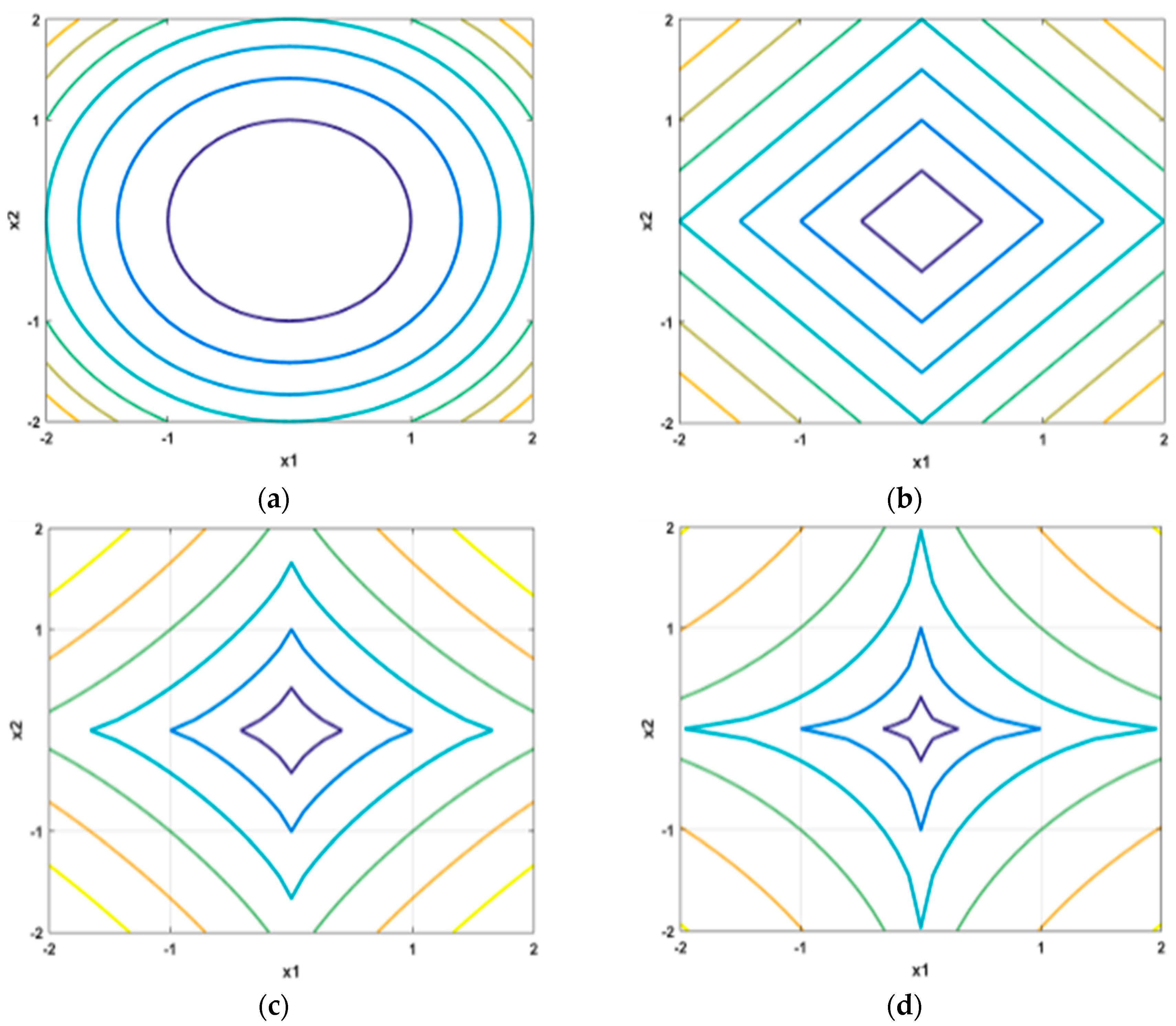
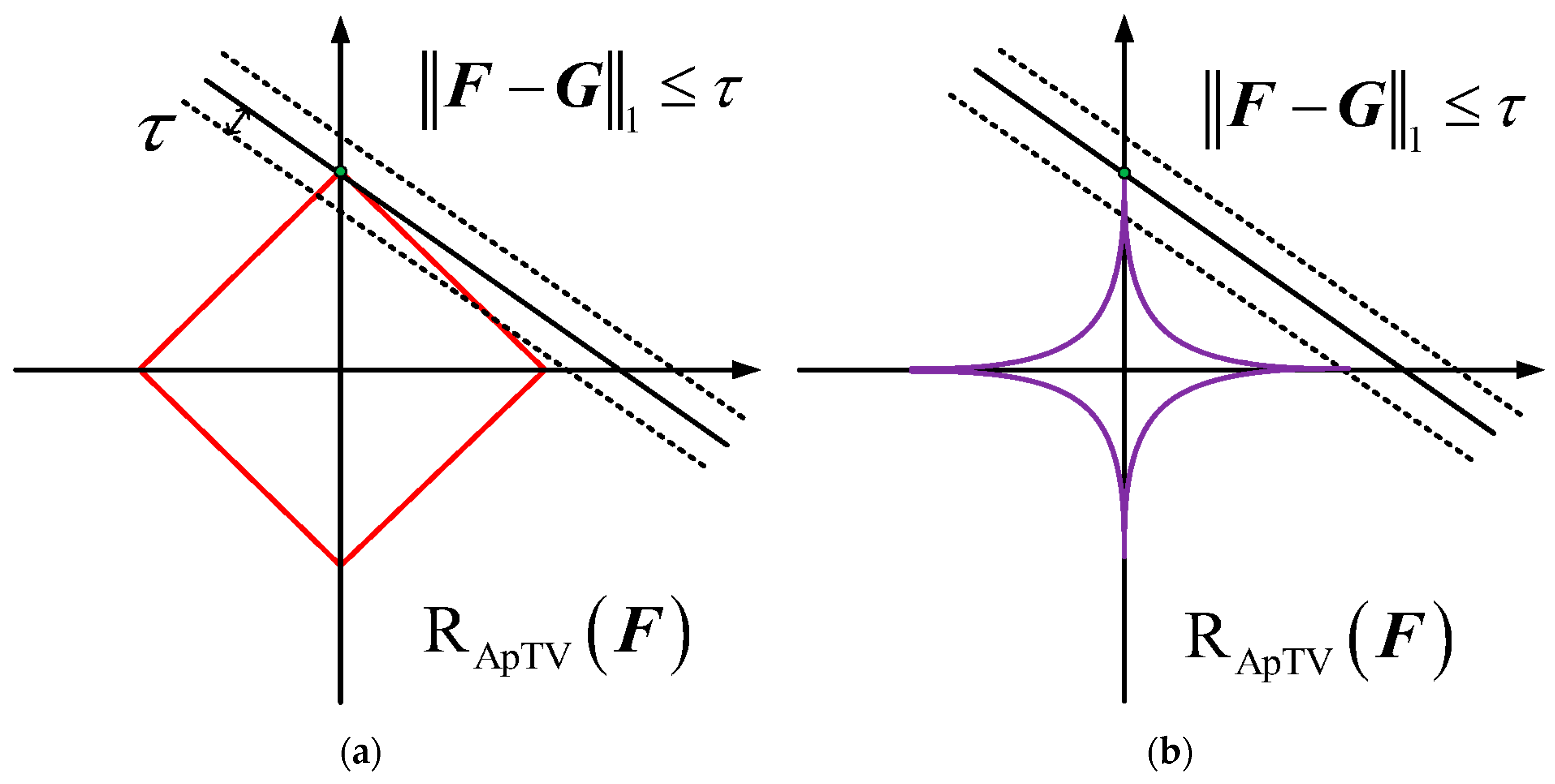
3.2. Overlapping Group Sparsity with Lp-Pseudo-Norm (OSG-Lp) Model

The L1-norm is commonly used as the fidelity term of impulse noise. However, the L1-norm is only the convex relaxation of the L0-norm. The p t h power of the Lp-norm ( 0 p 1 , for simplicity, we name it Lp-pseudo-norm) is another relaxation of the L0-norm. In fact, the L1-norm constraint is a particular case of the Lp-pseudo-norm.
Recently, the Lp-pseudo-norm [38,39,40,41,42] has attracted much attention in academia. Woodworth and Chartrand pointed out that the Lp-quasinorm is better for approximating the original L0-norm than the L1-norm and developed an iterative Lp-quasinorm shrinkage (LpS) solving the problem [43].
The Lp-pseudo-norm makes an improvement on the sparsity-based shrinkage operator by introducing another degree of freedom, thus giving the model a better ability to depict the sparsity of an image in the gradient domain, as shown in Figure 1.
Lp-pseudo-norm contour lines are given in Figure 1, where p = 2 and p = 1 represent L2- and L1-norms, respectively. Assuming that the image is contaminated by impulse noises with an absolute difference of τ, Figure 2 shows the schematic plots of anisotropic total variation contour lines R ApTV ( F ) = K h * F p p + K v * F p p ( 0 < p 1 ) intersecting with the fidelity term. As shown in Figure 2, the intersections of the contour lines with the fidelity term are more sparse for 0 < p < 1 , as shown in Figure 2b, than for p = 1 , as shown in Figure 2a, therefore the robustness of the model against noise is better.
Based on the above analysis, the advantages of Lp-quasinorm regularization are listed as follows: (1) The LpS operator may converge to an accurate solution. (2) The Lp-quasinorm is more flexible than the L1-norm. This might be useful to adapt the degree of sparsity to the signal being processed. (3) The Lp-quasinorm feasible domain makes the solution robust to noise.
Thus, the L1-norm-based OGS-TV could be extended to the Lp-pseudo-norm (abbreviated as OGS-Lp) [38,39,44] and is expressed as follows:
F = arg min F F G p p + μ [ φ ( K h * F ) + φ ( K v * F ) ] .  

4. Solution

4.1. Solving the OSG-Lp Model

The OSG-Lp model is treated as a minimization problem whose computation is given below. In real-life images, the values of all pixels usually fall in a limited interval [a, b]. For calculation and verification convenience, the image data are normalized so that they are all within [0, 1]. The operator PΩ is first defined with Ω = { F M × M | 0 F i , j 1 } .
  Ρ Ω ( F i , j ) = { 0 , F i , j < 0 , F i , j , F i , j [ 0 1 ] 1 , F i , j > 1 , .  
To solve the proposed model, we employed the ADMM framework and changed the complex problem into several subproblems. First, some intermediate variables were introduced to decouple the subproblems. That is, Z 1 = K h F , Z 2 = K v F , Z 3 = F G , Z 4 = F . then Equation (6) can be reformulated into the following constrained optimization problem:
F = arg min F i , j Ω Z 3 p p + μ [ φ ( Z 1 ) + φ ( Z 2 ) ] s . t . Z 1 = K h F , Z 2 = K v F , Z 3 = F G , Z 4 = F .
According to the principle of the ADMM framework, the Lagrange multipliers and the quadratic penalty term are needed to establish the augmented function. Then we have the following:
J ( F , Z 1 , Z 2 , Z 3 , Z 4 , β 1 , β 2 , β 3 , β 4 ) = Z 3 p p + μ [ φ ( Z 1 ) + φ ( Z 2 ) ] Λ 1 , ( Z 1 K h * F ) + β 1 2 Z 1 K h * F 2 2 Λ 2 , ( Z 2 K v * F ) + β 2 2 Z 2 K v * F 2 2 , Λ 3 , ( Z 3 F + G ) + β 3 2 Z 3 F + G 2 2 Λ 4 , ( Z 4 F ) + β 4 2 Z 4 F 2 2
where Λ 1 , Λ 2 , Λ 3 , Λ 4 are the Lagrange multipliers, and β1, β2, β3, β4 > 0 are the penalty coefficients. A , B is the inner-production operator of the matrixes A and B .
Introducing the scaled Lagrange multipliers Z ˜ 1 , Z ˜ 2 , Z ˜ 3 , Z ˜ 4 , which are also called dual variables.
Defined Z ˜ i ( i = 1 , 2 , 3 , 4 ) as following Z ˜ 1 = 1 β 1 Λ 1 , Z ˜ 2 = 1 β 2 Λ 2 , Z ˜ 3 = 1 β 3 Λ 3 , Z ˜ 4 = 1 β 4 Λ 4 . Add the term β i 2 ( Z ˜ i ) 2 β i 2 ( Z ˜ i ) 2 = 0 ( i = 1 , 2 , 3 , 4 ) to Equation (9) to complete the formula item. Equation (10) is obtained after rearrangement.
J ( F , Z 1 , Z 2 , Z 3 , Z 4 , β 1 , β 2 , β 3 , β 4 ) = Z 3 p p + μ [ φ ( Z 1 ) + φ ( Z 2 ) ] + β 1 2 Z 1 K h * F 2 2 β 1 Z ˜ 1 , Z 1 K h * F + β 1 2 ( Z ˜ 1 ) 2 β 1 2 ( Z ˜ 1 ) 2 + β 2 2 Z 2 K v * F 2 2 β 2 Z ˜ 2 , Z 2 K v * F + β 2 2 ( Z ˜ 2 ) 2 β 2 2 ( Z ˜ 2 ) 2 + β 3 2 Z 3 F + G 2 2 β 3 Z ˜ 3 , Z 3 F + G + β 3 2 ( Z ˜ 3 ) 2 β 3 2 ( Z ˜ 3 ) 2 + β 4 2 Z 4 F 2 2 β 4 Z ˜ 4 , Z 4 F + β 4 2 ( Z ˜ 4 ) 2 β 4 2 ( Z ˜ 4 ) 2 .
In Equation (10), the expressions
β i 2 Z i A 2 β i Z ˜ i , Z i A + β i 2 ( Z ˜ i ) 2 ( i = 1 , 2 , 3 , 4 ) ,  
satisfy the form of a 2 2 a b + b 2 = ( a b ) 2 , so Equation (10) can be written as Equation (12):
J ( F , Z 1 , Z 2 , Z 3 , Z 4 , β 1 , β 2 , β 3 , β 4 ) = Z 3 p p + μ φ ( Z 1 ) + μ φ ( Z 2 ) + β 1 2 Z 1 K h * F Z ˜ 1 2 2 + β 2 2 Z 2 K v * F Z ˜ 2 2 2 + β 3 2 Z 3 F + G Z ˜ 3 2 2 + β 4 2 Z 4 F Z ˜ 4 2 2 β 1 2 ( Z ˜ 1 ) 2 β 2 2 ( Z ˜ 2 ) 2 β 3 2 ( Z ˜ 3 ) 2 β 4 2 ( Z ˜ 4 ) 2 .
Because Z 1 , Z 2 , Z 3 , Z 4 , Z ˜ 1 , Z ˜ 2 , Z ˜ 3 , Z ˜ 4 are mutually independent, so, they can be solved as some independent subproblems according to the principle of the ADMM algorithm. These problems can be solved by the iterative algorithm for minimizing Z i .
Defining Z i ( k ) ( i = 1 , 2 , 3 , 4 ) represents the value of Z i after ( k ) t h iterations. For a given Z i ( k ) , the next iteration Z i ( k + 1 ) is generated as follows:
Z 1 ( k + 1 ) = arg min Z 1 μ φ ( Z 1 ) + β 1 2 Z 1 K h * F ( k ) Z ˜ 1 ( k ) 2 2 .  
Z 2 ( k + 1 ) = arg min Z 2 μ φ ( Z 2 ) + β 2 2 Z 2 K v * F ( k ) Z ˜ 2 ( k ) 2 2 .  
Z 3 ( k + 1 ) = arg min Z 3 Z 3 p p + β 3 2 Z 3 F ( k ) + G Z ˜ 3 ( k ) 2 2 .  
Z 4 ( k + 1 ) = arg min Z 4 β 4 2 Z 4 F ( k ) Z ˜ 4 ( k ) 2 2 .  
Each of these four equations are solved below:
(1) The Z 1 ( k + 1 ) and the Z 2 ( k + 1 ) are solved by the majorization-minimization (MM) algorithm [33], which approximates the solution of the target problem by finding a well-behaving multi-variable auxiliary function and constructing an iterative sequence.
First, suppose a minimization optimization problem with the following form:
min v P ( v ) = { α 2 v v 0 2 2 + φ ( v ) } , v M 2 × 1 ,  
where α > 0 and φ (v) satisfies φ ( v ) = i = 1 N j = 1 N v ˜ i , j , N , N 2 . To avoid having to solve the complex minimization problem P(v) directly, a function Q(v, u) for which Q(v, u) ≥ P(v) for all v , u could be constructed. The equality sign holds if and only if u = v. Thus, the optimal solution of P(v) is the minimum value of Q(v, u). Generally, an MM iterative algorithm for minimizing P(v) has the form:
v ( n + 1 ) = arg min v Q ( v , v ( n ) ) ,
It can be solved step-by-step in the following way.
The properties of the function φ ( v ) = i = 1 N j = 1 N v ˜ i , j , N , N 2  are first observed. It is known that the equality sign holds when u = v, as shown in Equation (19):
1 2 ( 1 u 2 v 2 2 + u 2 ) v 2  
which means φ ( v )  can be solved by constructing the function S(v) of Equation (20):
S ( v , u ) = 1 2 i = 1 N j = 1 N [ 1 u ˜ i , j , N , N 2 v ˜ i , j , N , N 2 2 + u ˜ i , j , N , N 2 ] φ ( v ) = i = 1 N j = 1 N v ˜ i , j , N , N 2 .
After a simple calculation [31], S ( v , u ) is rewritten as
S ( v , u ) = 1 2 D ( u ) v 2 2 + C ( u )  
to facilitate future calculations.
C ( u ) in the above equation is independent of v , and D ( u ) M 2 × M 2 is a diagonal matrix with its elements defined as
[ D ( u ) ] m , m = i = N l N r j = N l N r [ k 1 = N l N r k 2 = N l N r | u m i + k 1 , m i + k 2 | 2 ] 1 2 ( m = 1 , 2 , , M 2 )  
The entries of D can be easily computed by using MATLAB built-in function “conv2”. Putting Equations (17), (21), and (22) together, the optimization problem P ( v ) can be written as
Q ( v , u ) = α 2 v v 0 2 2 + S ( v , u ) = α 2 v v 0 2 2 + 1 2 D ( u ) v 2 2 + C ( u ) .  
When v = u , Q ( u , u ) = P ( u ) , to minimize P ( v ) , the MM aims to iteratively solve
v ( n + 1 ) = arg min v α 2 v v 0 2 2 + 1 2 D ( v ( n ) ) v 2 2 , n = 1 , 2 , 3  
with the solution
v ( n + 1 ) = ( I + 1 α D 2 ( v ( n ) ) ) 1 v 0 , n = 1 , 2 , 3 ,  
where I M 2 × M 2 is an identity matrix with the same size of D 2 ( v ( n ) ) , D 2 ( v ( n ) ) is also a diagonal matrix which has the same form of Equation (22).
Observing functions of Equations (13) and (14), the subproblem Z 1 , Z 2 conforms to the function in Equation (17) and can be solved iteratively using Equation (26). Z i ( n + 1 ) ( k + 1 ) ( i = 1 , 2 ) represents the ( n ) -th iteration of the MM algorithm in the ( k + 1 ) -th outer loop.
Z i ( n + 1 ) ( k + 1 ) = m a t { [ I + μ β i D 2 ( Z i ( n ) ( k + 1 ) ) ] 1 z i ( 0 ) ( k + 1 ) } , ( i = 1 , 2 ) ,  
where m a t plays the role of reshaping a vector to a matrix and z i ( 0 ) ( k + 1 ) is the vector form of Z i ( 0 ) ( k + 1 ) .
The initial values of Z 1 ( 0 ) ( k + 1 ) Z 2 ( 0 ) ( k + 1 ) in the above equation are:
{ Z 1 ( 0 ) ( k + 1 ) = K h * F ( k ) + Z ˜ 1 ( k ) Z 2 ( 0 ) ( k + 1 ) = K v * F ( k ) + Z ˜ 2 ( k ) .  
(2) Z 3 ( k + 1 ) could be solved by the famous soft thresholding shrinkage method [45] as shown below:
Z 3 ( k + 1 ) = arg min Z 3 Z 3 p p + β 3 2 Z 3 F ( k ) + G Z ˜ 3 ( k ) 2 2 = s h r i n k a g e ( F ( k ) G + Z ˜ 3 ( k ) , 1 β 3 , p ) = sign ( F ( k ) G + Z ˜ 3 ( k ) ) . * max ( abs ( F ( k ) G + Z ˜ 3 ( k ) ) ( 1 β 3 ) . ^ ( p 2 ) . * abs ( F ( k ) G + Z ˜ 3 ( k ) ) . ^ ( p 1 ) , 0 ) .
(3) The Z 4 ( k + 1 ) subproblem is computed as
Z 4 ( k + 1 ) = arg min Z 4 β 4 2 Z 4 F ( k ) Z ˜ 4 ( k ) 2 2 = min ( 1 , max ( F ( k ) + Z ˜ 4 ( k ) , 0 ) ) , .
(4) The F ( k + 1 ) subproblem is solved by substituting Z 1 ( k + 1 ) , Z 2 ( k + 1 ) , Z 3 ( k + 1 ) , Z 4 ( k + 1 ) into Equation (12) and calculating for the variable F ( k + 1 ) . Under the assumption of periodic boundary conditions, fast Fourier transform is applied to both sides of the equation to perform the computation in the frequency domain instead of a spatial domain, in order to reduce the computational complexity caused by matrix multiplication. Matrix multiplication is converted to dot product operation, in other words, solving the following normal equation:
( β 1 K ¯ h * . * K ¯ h + β 2 K ¯ v * . * K ¯ v + β 3 1 + β 4 1 ) . * F ¯ ( k + 1 ) = β 1 K ¯ h * . * ( Z ¯ 1 ( k + 1 ) Z ˜ ¯ 1 ( k ) ) + β 2 K ¯ v * . * ( Z ¯ 2 ( k + 1 ) Z ˜ ¯ 2 ( k ) ) + β 3 ( Z ¯ 3 ( k + 1 ) + G ¯ Z ˜ ¯ 3 ( k ) ) + β 4 ( Z ¯ 4 ( k + 1 ) Z ˜ ¯ 4 ( k ) )
where x ¯ is the frequency-domain representation of x , “ . * ” stands for dot product, “*“ is the conjugate, 1 is the matrix whose entries are all 1, and represents the two-dimensional fast Fourier transform (FFT). Rearranging of the equation gives F ( k + 1 ) as
F ( k + 1 ) = 1 ( β 1 K ¯ h * . * ( Z ¯ 1 ( k + 1 ) Z ˜ ¯ 1 ( k ) ) + β 2 K ¯ v * . * ( Z ¯ 2 ( k + 1 ) Z ˜ ¯ 2 ( k ) ) + β 3 ( Z ¯ 3 ( k + 1 ) + G ¯ Z ˜ ¯ 3 ( k ) ) + β 4 ( Z ¯ 4 ( k + 1 ) Z ˜ ¯ 4 ( k ) ) β 1 K ¯ h * K ¯ h + β 2 K ¯ v * K ¯ v + β 3 1 + β 4 1 ) .
(5) The dual variables Z ˜ 1 , Z ˜ 2 , Z ˜ 3 , Z ˜ 4 could be updated via the gradient ascent method.
{ Z ˜ 1 ( k + 1 ) = Z ˜ 1 ( k ) + γ β 1 ( K h * F ( k + 1 ) Z 1 ( k + 1 ) ) Z ˜ 2 ( k + 1 ) = Z ˜ 2 ( k ) + γ β 2 ( K v * F ( k + 1 ) Z 2 ( k + 1 ) ) Z ˜ 3 ( k + 1 ) = Z ˜ 3 ( k ) + γ β 3 ( F ( k + 1 ) G Z 3 ( k + 1 ) ) Z ˜ 4 ( k + 1 ) = Z ˜ 4 ( k ) + γ β 4 ( F ( k + 1 ) Z 4 ( k + 1 ) ) .  

4.2. OGS-Lp-FAST Model

The denoising models based on OGS is more time consuming than the TV-based model. This is mainly because that OGS model considers the gradient information of the neighborhood in a reconstructed image, thus making the computation more complex. Thus, this is a shortcoming.
Goldstein et al. [12] proposed an accelerated ADMM algorithm with a restart that improves the convergence rate of the ADMM algorithm from O ( 1 k ) to O ( 1 k 2 ) . Inspired by them, we adopted this algorithm to improve the OGS-Lp model. This modified model is named OGS-Lp-FAST (“Ours” for short). The auxiliary variables U i ( i = 1 , 2 ) and U ˜ i ( i = 1 , 2 ) are first adopted. Under this framework, Z i ( i = 1 , 2 , 3 , 4 ) is updated in the following way:
{ Z 1 ( n + 1 ) ( k + 1 ) = m a t { [ I + μ β 1 D 2 ( v ( n ) ) 2 ( Z 1 ( n + 1 ) ( k + 1 ) ) ] 1 z 1 ( 0 ) ( k + 1 ) } Z 2 ( n + 1 ) ( k + 1 ) = m a t { [ I + μ β 2 D 2 ( v ( n ) ) ( Z 2 ( n + 1 ) ( k + 1 ) ) ] 1 z 2 ( 0 ) ( k + 1 ) } Z 3 ( k + 1 ) = s h r i n k a g e ( F ( k ) G + Z ˜ 3 ( k ) , 1 β 3 , p ) Z 4 ( k + 1 ) = m i n ( 1 , m a x ( F ( k ) + Z ˜ 4 ( k ) , 0 ) ) , .  
The initial values of Z 1 ( 0 ) ( k + 1 ) Z 2 ( 0 ) ( k + 1 ) in the above equation are:
{ Z 1 ( 0 ) ( k + 1 ) = K h * F ( k ) + U ˜ 1 ( k ) Z 2 ( 0 ) ( k + 1 ) = K v * F ( k ) + U ˜ 2 ( k ) .  
The dual variable Z ˜ i ( i = 1 , 2 ) can be updated as follows:
{ Z ˜ 1 ( k + 1 ) = U ˜ 1 ( k ) + γ β 1 ( K h * F ( k ) Z 1 ( k + 1 ) ) Z ˜ 2 ( k + 1 ) = U ˜ 2 ( k ) + γ β 2 ( K v * F ( k ) Z 2 ( k + 1 ) ) Z ˜ 3 ( k + 1 ) = Z ˜ 3 ( k ) + γ β 3 ( F ( k ) G Z 3 ( k + 1 ) ) Z ˜ 4 ( k + 1 ) = Z ˜ 4 ( k ) + γ β 4 ( F ( k ) Z 4 ( k + 1 ) ) .  
As image denoising is not a strong convex problem, the iteration needs to be restarted to ensure the convergence of the algorithm. When Equation (33) is not satisfied, the algorithm is restarted.
c i ( k ) < η c i ( k 1 ) ( i = 1 , 2 ) ,  
where c i ( k ) = β 1 Z ˜ i ( k ) U ˜ i ( k ) 2 2 + β Z i ( k ) U i ( k ) 2 2 is the sum of the ( k ) - t h primal residuals β Z i ( k ) U i ( k ) 2 2 and the dual residuals β 1 Z ˜ i ( k ) U ˜ i ( k ) 2 2 , and η is a number close to 1. To prevent frequent restarts, η = 0.97 is set.
When c i ( k ) < η c i ( k 1 ) , the acceleration step size is set to ε i , and the auxiliary variables U i ( i = 1 , 2 ) and U ˜ i ( k + 1 ) ( i = 1 , 2 ) are updated as follows:
{ ε i ( k + 1 ) = 1 + 1 + 4 ( ε i ( k ) ) 2 2 ( i = 1 , 2 ) U i ( k + 1 ) = Z i ( k + 1 ) + ε i ( k ) 1 ε i ( k + 1 ) ( Z i ( k + 1 ) Z i ( k ) ) ( i = 1 , 2 ) U ˜ i ( k + 1 ) = Z ˜ i ( k + 1 ) + ε i ( k ) 1 ε i ( k + 1 ) ( Z ˜ i ( k + 1 ) Z ˜ i ( k ) ) ( i = 1 , 2 ) .  
which is updated according to the equations below upon restart:
{ ε i ( k + 1 ) = 1 ( i = 1 , 2 ) U i ( k + 1 ) = Z i ( k + 1 ) ( i = 1 , 2 ) U ˜ i ( k + 1 ) = Z ˜ i ( k + 1 ) ( i = 1 , 2 ) c i ( k + 1 ) = η 1 c i ( k ) ( i = 1 , 2 ) .  
Up to this point, all subproblems of the proposed model are solved. The OGS-Lp-FAST algorithm just described is summarized as Algorithm 1.
The F sub-problem should be updated as
F ( k + 1 ) = 1 ( β 1 K ¯ h * . * ( U ¯ 1 ( k + 1 ) U ˜ ¯ 1 ( k + 1 ) ) + β 2 K ¯ v * . * ( U ¯ 2 ( k + 1 ) U ˜ ¯ 2 ( k + 1 ) ) + β 3 ( Z ¯ 3 ( k + 1 ) + G ¯ Z ˜ ¯ 3 ( k + 1 ) ) + β 4 ( Z ¯ 4 ( k + 1 ) Z ˜ ¯ 4 ( k + 1 ) ) β 1 K ¯ h * K ¯ h + β 2 K ¯ v * K ¯ v + β 3 1 + β 4 1 ) .
Algorithm 1 OGS-Lp-FAST pseudo-code
Input: image G with noise
Output: denoised image F
Initialize:
k = 1 , n = 0 , Z i ( k ) = 0 , Z ˜ i ( k ) = 0 ( i = 1 , 2 , , 4 ) , β 1 , β 2 , β 3 , β 4 , μ , p , η , U j ( k ) = 0 , U ˜ j ( k ) = 0 ( j = 1 , 2 ) , γ , t o l , c 1 = i n f , F ( k ) = G , M a x
1: for k = 1 : M a x
2: If : c i ( k + 1 ) < η c i ( k ) :
3: Z i ( k + 1 ) , ( i = 1 , 2 , 3 , 4 ) , are updated with Equations (33) and (34)
4: Z ˜ i ( k + 1 ) ( i = 1 , 2 , 3 , 4 ) are updated with Equation (35)
5: ε i ( k + 1 ) , U j ( k + 1 ) , U ˜ j ( k + 1 ) ( j = 1 , 2 ) is updated with Equation (37)
6: F ( k + 1 ) are updated with Equation (39)
7: E = F ( k + 1 ) F ( k ) 2 / F ( k ) 2
8 Else
9: Restart as in Equation (38)
10: End If
11: If E < tol Break;
12: End For
13: Return F(k) as F

5. Experimental Results and Analyses

In this section, eight typical grayscale images with a size of 256 × 256 pixels are chosen to validate the denoising performance of the Lp-OSG-TV-FAST method. The test images are as shown in Figure 3. The image “House” is downloaded from http://sipi.usc.edu/database/database.php?volume%92=%92misc&image=5top. The images “Lena“ and “Pepper” are from http://decsai.ugr.es/cvg/dbimagenes/. The images “Woman”, “Girl”, and “Reagan” are from http://www.hlevkin.com/default.html#testimages. The images “Milk drop” and “Shoulder” are from http://www.cs.cmu.edu/~cil/v-images.html. The versions of the images in our paper are other special formats which are converted by Photoshop from the sources above.
The method proposed here is compared with ATV, ITV, TGV, OSG-L1, and OGS-Lp methods, and is evaluated objectively in terms of the peak signal-to-noise ratio (PSNR), structural similarity (SSIM), runtime, and other experimental indicators [45]. Simulations are performed on MATLAB R2014a platform running in a hardware environment of Inter(R) Core (TM) [email protected] CPU and 16 GB memory.

5.1. Evaluation Method

In the denoising field, the common evaluating criteria including PSNR, SSIM, and runtime. The PSNR and SSIM [46] are defined in Equations (40) and (41):
P S N R ( X , Y ) = 10 lg ( M A X ( X ) ) 2 1 N 2 i = 1 N j = 1 N ( X i j Y i j ) 2  
where X denotes the original image, Y is the reconstructed image, and M A X ( X ) represents the largest gray value in the original image.
S S I M ( X , Y ) = ( 2 u X u Y + ( L k 1 ) 2 ) ( 2 σ X Y + ( L k 2 ) 2 ) ( u X 2 + u Y 2 + ( L k 1 ) 2 ) ( σ X 2 + σ Y 2 + ( L k 2 ) 2 )  
where u X is the mean of X ; u Y is the mean of Y ; σ X 2 is the variance of X ; σ Y 2 is the variance of Y ; σ X Y is the covariance between X and Y ; and L = 512 , k 1 = 0.05 , k 2 = 0.05 . The parameter L = 255 .

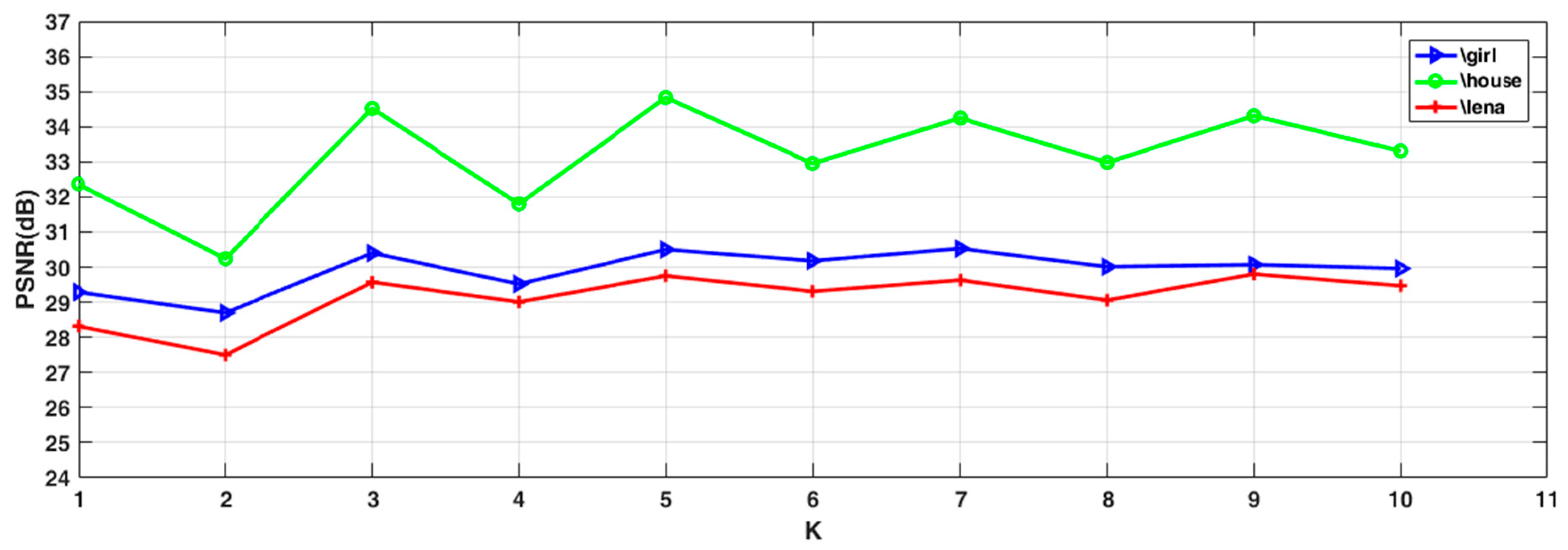
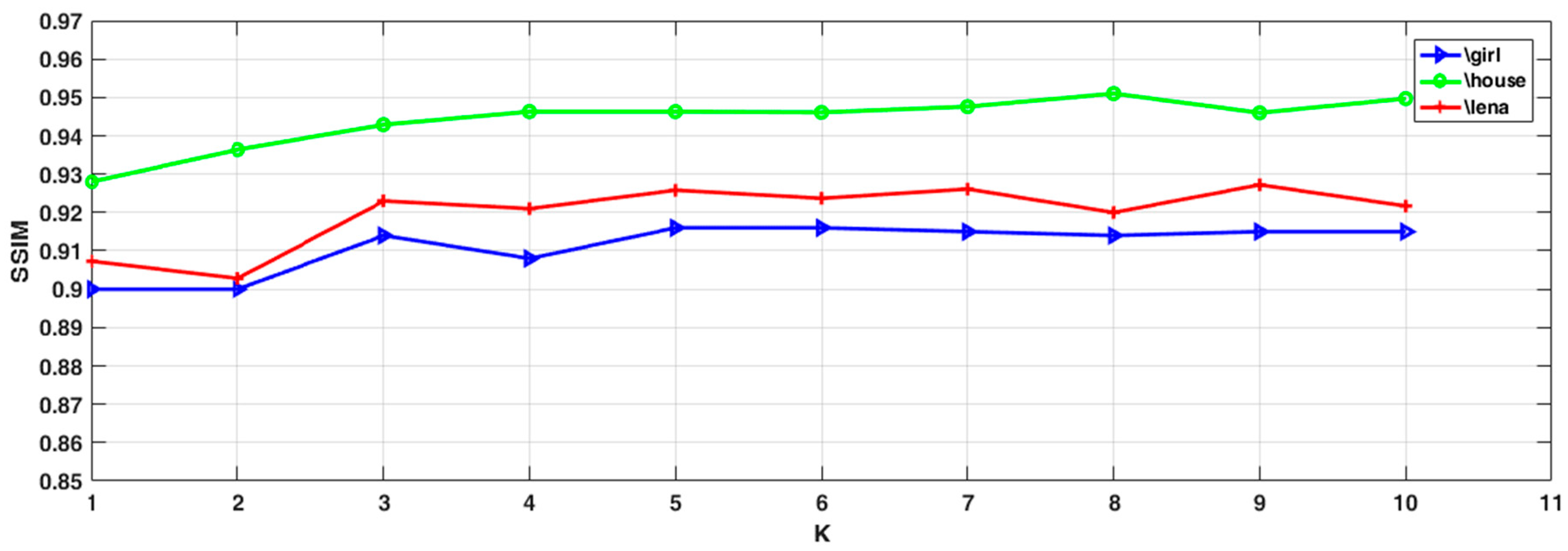
5.2. Sensitivity of the Parameters

In this section, an important parameter of the proposed algorithm, the group size K, is tested and compared to evaluate its overall effect on the algorithm. PSNR and SSIM are used as criteria to evaluate the algorithm objectively. Three images (“Girl”, “House”, and “Lena”) with 30% noise level are selected, on which K is made to vary continuously from 1 to 10. The other parameters are adjusted to the optimum. PSNR and SSIM values are recorded and plotted into graphs, as shown in Figure 4 and Figure 5. In Figure 4, PSNR and SSIM increase with the increase of K and reach their maximum at K = 5. Further increases in K leads to decreased PSNR values. Thus, the neighborhood information of an image has a positive impact on the performance of the algorithm. With K set to appropriate values, the edge information of the image is better preserved, and the noise resistance is improved. However, K should not be too large either, or nearby regions with drastic pixel changes could be taken, which will result in decreased PSNR and SSIM.
Then, we tested how to select a good regularization parameter μ for different images. We started with the value of μ from a low value then increased the parameters empirically as the level of noise improved to get the best visual effect. For example, for the “Girl” image corrupted by impulse noise from 20% to 50%, μ = 0.14, 0.15, 0.15, 0.18, respectively.
In the selection of the parameter p , the p value is set between 0 and 1. On the premise of fixing other parameters, we increase p by 0.1 step. After several rounds of experiments, we select the optimal when the image gets the best visual effect.
The optimal parameters for different images with the noise level from 20% to 50% are given in Table 1.

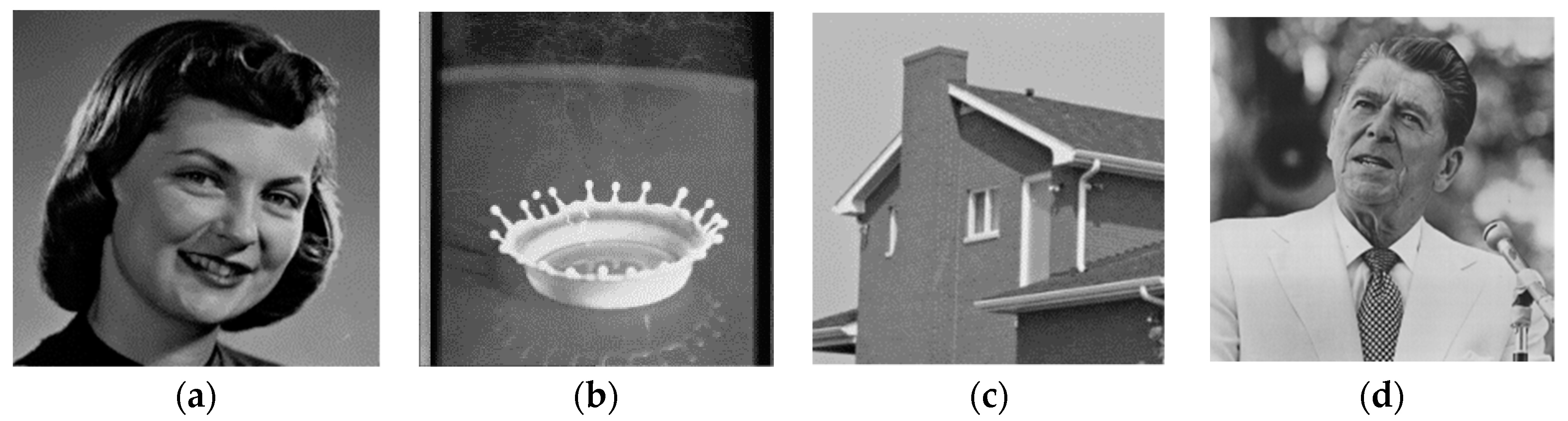
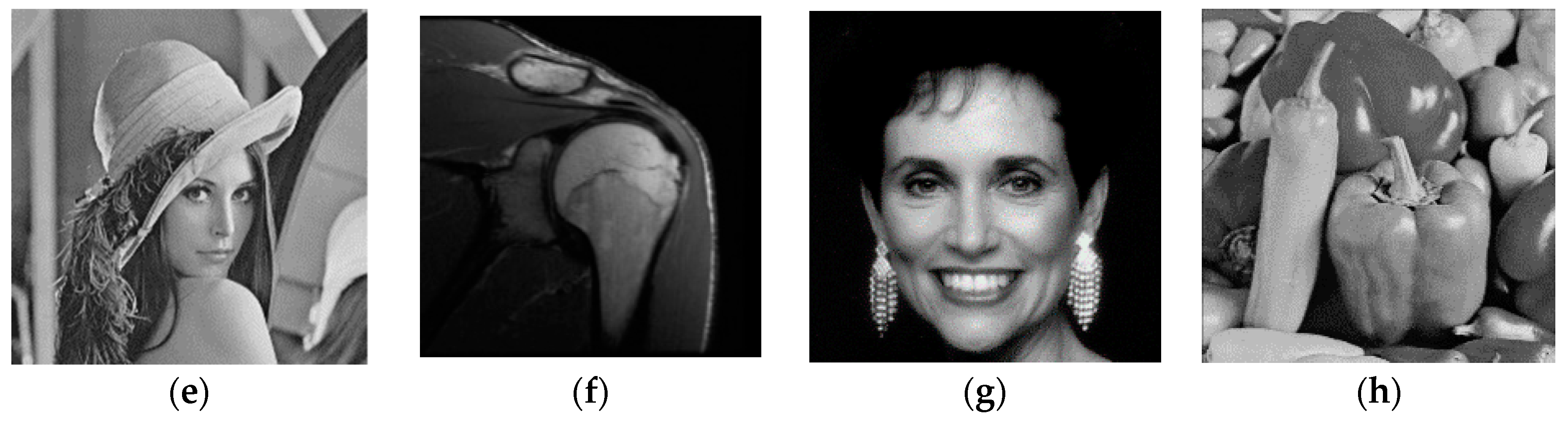
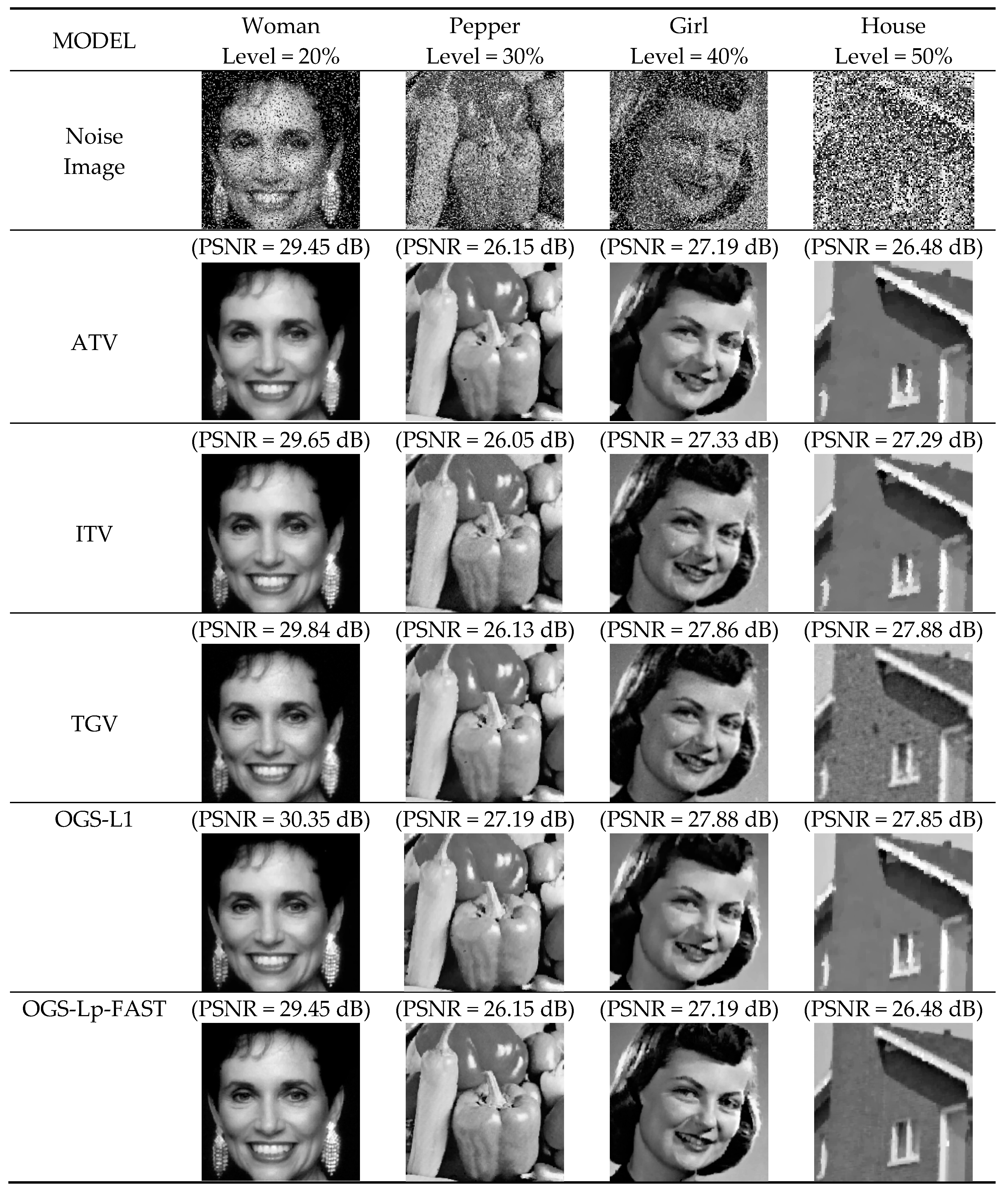
5.3. Testing and Comparing the Denoising Performance of Different Algorithms

Six images are selected from the original images of Figure 3 for testing, on which impulse noise at levels from 20% to 50%, to compare the denoising effects of ATV, ITV, TGV, OGS-L1, OGS-Lp, and Ours algorithms (six in total). To ensure the objectiveness and fairness of the evaluation, the above algorithms all adopt the following iterative condition:
F ( k + 1 ) F ( k ) 2 F ( k ) 2 1 < 1 0 4 .  
Regularization parameters of these algorithms are adjusted to ensure the best denoising effect of each, which ensured the fairness of the test. For methods based on the OGS model, the group size is set to K = 5. The test results on different images are given in Table 2, Table 3, Table 4 and Table 5. The best indicator values are labeled as black and bold. By observing the data in each table, the following conclusions could be made:
  • With the introduction of different levels of noise to the images, our model generates higher PSNR and SSIM values for the reconstructed images than other methods, indicating its superior denoising effect. The recovered images also resemble the original ones more.
  • The proposed model works better at lower noise levels. For example, at a 20% noise level, as shown in Table 2, the PSNR value of the “House” image (37.72 dB) given by our model is 5.91 dB higher than that given by the ITV model (31.81 dB) and 5.4 dB higher than that of the TGV model (32.32 dB). Even at high noise levels, our model still performs better than the others, which shows the clear advantages that total variation with overlapping group sparsity has over the classic anisotropic TV model.
  • Compared to OGS-L1, our proposed method incorporates the Lp-pseudo-norm shrinkage, which adds another degree of freedom to the algorithm and improves the depiction of the gradient-domain sparsity of the images, achieving a better denoising effect. For example, at a 20% noise level, as shown in Table 2, the PSNR value of the “Girl” image (32.34 dB) given by our model is 1.67 dB higher than that given by the OGS-L1 model (30.67 dB). Even at a noise level of 50%, as shown in Table 5, the PSNR value of the “Girl” image (27.35 dB) given by our model is still 0.90 dB higher than that given by the OGS-L1 model (26.45 dB). This proves that the Lp-pseudo-norm is more suitable as a regularizer for describing the sparsity of images than the L1-norm.
  • In terms of the runtime of the six models, the OGS-based method is more time consuming than ATV, ITV, and TGV. This is mainly because the OGS model considers the gradient information of the neighborhood in an image undergoing reconstruction, thus making the computation more complex.
  • Comparing the values of PSNR and SSIM in Table 2, Table 3, Table 4 and Table 5, OGS-Lp-FAST and OGS-Lp have the same denoising effect. However, by observing the value of runtime of all testing images, we find that convergence is sped up in the OGS-LP-FAST method with the use of accelerated ADMM with a restart. For example, at a 20% noise level, as shown in Table 2, the time value of the “Woman” image (8.69 s) given by the OGS-Lp-FAST model is 7.53 s less than that given by the OGS-L1 model (16.22 s).
To verify our proposed method further, we compared the image details restored by different algorithms. Figure 6 shows four images (“Woman”, “Pepper”, “Girl”, and “House”) with impulse noise from 20% to 50%. The enlarged details of the images restored by ATV, ITV, TGV, OGS-L1, and OGS-Lp-FAST algorithms are displayed for comparison.
In terms of the visual effect of the restored images, ATV denoising produces apparent blocking artifacts in the images. In the “Pepper” image ATV recovers, we can easily find two heavy noise pixels.
The ITV method also shows significant staircase effect. In the “House” image it restores, the edge of the image is not well preserved when the noise pollution is high.
For the denoising results of TGV, the blocking artifacts in the images are sufficiently suppressed, but local heavy noise spots are still observable.
Finally, by comparing the four images, we can easily see the visual improvement in the images by using our method. Even at high noise pollution, our method protects the edge information of the image very well, and at the same time, avoids the staircase effect.

6. Discussion and Conclusions

In this work, we study a new regularization model by applying TV with OGS and Lp-pseudo-norm shrinkage for the image polluting under impulse noise. We provided the efficient algorithm OGS-Lp-FAST under the ADMM framework. This algorithm is rooted in overlapping group sparsity-based regularization, and incorporated the comparisons made with ATV, ITV, TGV, OGS-L1, and OGS-Lp models for validation of our proposed method. The following conclusions are drawn from the experimental results:
  • An overlapping group sparsity (OGS)-based regularizer is used to replace the anisotropic total variation (ATV), to describe the prior conditions of the image. OGS makes full use of the similarity among image neighborhoods and the dissimilarity in the surroundings of each point. It promotes the distinction between the smooth and edge regions of an image, thus enhancing the robustness of the proposed model.
  • Lp-pseudo-norm shrinkage is used in place of the L1-norm regularization to describe the fidelity term of images with salt and pepper noise. With the inclusion of another degree of freedom, Lp-pseudo-norm shrinkage reflects the sparsity of the image better and greatly improves the denoising performance of the algorithm.
  • The difference operator is used for convolution. Under the ADMM framework, the complex model is transformed into a series of simpler mathematical problems to solve.
  • Appropriate K values could effectively improve the overall denoising performance of the model. In practice, this parameter needs to be adjusted. If it is too small, the neighborhood information is not utilized completely. If the value is too big, too many dissimilar pixel blocks will be included, impairing the denoising result.
  • The adoption of accelerated ADMM with a restart accelerates the convergence of the algorithm. The running time is reduced.
  • In this paper, we focus on impulse noise removal, but the model is also applicable to other types of noise removal that we will further study in future work.

Author Contributions

Funding acquisition, F.Y.; Methodology, L.W., Y.C. (Yingpin Chen) and F.L.; Software, L.W., Y.C. (Yingpin Chen) and Y.C. (Yuqun Chen) and Z.C.; Writing—original draft, L.W.; Writing—review & editing, Y.C. (Yingpin Chen).

Funding

This work is supported by the Foundation of Fujian Province Great Teaching Reform [FBJG20180015], the Education and Scientific Research Foundation of Education Department of Fujian Province for Middle-aged and Young Teachers [grant number JT180309],the Education and Scientific Research Foundation of Education Department of Fujian Province for Middle-aged and Young Teachers [grant number JAT170352], the Foundation of Department of Education of Guangdong Province [2017KCXTD015], and the Open Foundation of Digital Signal and Image Processing Key Laboratory of Guangdong Province [grant number 2017GDDSIPL-01], the Education and Scientific Research Foundation of Education Department of Fujian Province for Middle-aged and Young Teachers [grant number JT180310], the Education and Scientific Research Foundation of Education Department of Fujian Province for Middle-aged and Young Teachers [grant number JT180311].

Conflicts of Interest

The authors declare no conflict of interest.

References

  1. He, W.; Zhang, H.; Zhang, L.; Shen, H. Total-Variation-Regularized Low-Rank Matrix Factorization for Hyperspectral Image Restoration. IEEE Trans. Geosci. Remote Sens. 2015, 54, 178–188. [Google Scholar] [CrossRef]
  2. Cevher, V.; Sankaranarayanan, A.; Duarte, M.F.; Reddy, D.; Baraniuk, R.G.; Chellappa, R. Compressive Sensing for Background Subtraction; Springer: Berlin/Heidelberg, Germany, 2008; pp. 155–168. [Google Scholar]
  3. Huang, G.; Jiang, H.; Matthews, K.; Wilford, P. Lensless imaging by compressive sensing. In Proceedings of the IEEE International Conference on Image Processing, Melbourne, VIC, Australia, 15–18 September 2014; pp. 2101–2105. [Google Scholar]
  4. Chen, Y.; Peng, Z.; Cheng, Z.; Tian, L. Seismic signal time-frequency analysis basedon multi-directional window using greedy strategy. J. Appl. Geophys. 2017, 143, 116–128. [Google Scholar] [CrossRef]
  5. Lu, S.L.T.; Fang, L. Spectral–spatial adaptive sparse representation for hyperspectral image denoising. IEEE Trans. Geosci. Remote Sens. 2016, 54, 373–385. [Google Scholar] [CrossRef]
  6. Zhao, W.; Lu, H. Medical Image Fusion and Denoising with Alternating Sequential Filter and Adaptive Fractional Order Total Variation. IEEE Trans. Instrum. Meas. 2017, 66, 1–12. [Google Scholar] [CrossRef]
  7. Knoll, F.; Bredies, K.; Pock, T.; Stollberger, R. Second order total generalized variation (TGV) for MRI. Magn. Reson. Med. 2011, 65, 480–491. [Google Scholar] [CrossRef] [PubMed]
  8. Kong, D.; Peng, Z. Seismic random noise attenuation using shearlet and total generalized variation. J. Geophys. Eng. 2015, 12, 1024–1035. [Google Scholar] [CrossRef]
  9. Zhu, Z.; Yin, H.; Chai, Y.; Li, Y.; Qi, G. A novel multi-modality image fusion method based on image decomposition and sparse representation. Inform. Sci. 2018, 432, 516–529. [Google Scholar] [CrossRef]
  10. Marquina, A.; Osher, S.J. Image super-resolution by TV-regularization and Bregman iteration. J. Sci. Comput. 2008, 37, 367–382. [Google Scholar] [CrossRef]
  11. Nikolova, M. A variational approach to remove outliers and impulse noise. J. Math. Imaging Vis. 2004, 20, 99–120. [Google Scholar] [CrossRef]
  12. Rudin, L.I.; Osher, S.; Fatemi, E. Nonlinear total variation based noise removal algorithms. Phys. D Nonlinear Phenom. 1992, 60, 259–268. [Google Scholar] [CrossRef]
  13. Qin, Z. An Alternating Direction Method for Total Variation Denoising. Optim. Methods Softw. 2015, 30, 594–615. [Google Scholar] [CrossRef]
  14. Tai, X.C.; Wu, C. Augmented Lagrangian Method, Dual Methods and Split Bregman Iteration for ROF Model. In International Conference on Scale Space and Variational Methods in Computer Vision; Springer: Berlin/Heidelberg, Germany, 2009; pp. 502–513. [Google Scholar]
  15. Ng, M.; Wang, F.; Yuan, X.M. Fast Minimization Methods for Solving Constrained Total-Variation Superresolution Image Reconstruction. Multidimens. Syst. Signal Process. 2011, 22, 259–286. [Google Scholar] [CrossRef]
  16. Chan, T.; Marquina, A.; Mulet, P. High-order total variation-based image restoration. SIAM J. Sci. Comput. 2000, 22, 503–516. [Google Scholar] [CrossRef]
  17. Chan, T.F.; Esedoglu, S.; Park, F. A fourth order dual method for staircase reduction in texture extraction and image restoration problems. In Proceedings of the 2010 17th IEEE International Conference on Image Processing (ICIP), Hong Kong, China, 26–29 September 2010; pp. 4137–4140. [Google Scholar]
  18. Wu, L.; Chen, Y.; Jin, J.; Du, H.; Qiu, B. Four-directional fractional-order total variation regularization for image denoising. J. Electron. Imaging 2017, 26, 053003. [Google Scholar] [CrossRef]
  19. Bredies, K.; Kunisch, K.; Pock, T. Total generalized variation. SIAM J. Imaging Sci. 2010, 3, 492–526. [Google Scholar] [CrossRef]
  20. Feng, W.; Lei, H.; Gao, Y. Speckle reduction via higher order total variation approach. IEEE Trans. Image Process. 2014, 23, 1831–1843. [Google Scholar] [CrossRef] [PubMed]
  21. Cheng, Z.; Chen, Y.; Wang, L.; Lin, F.; Wang, H.; Chen, Y. Four-Directional Total Variation Denoising Using Fast Fourier Transform and ADMM. In Proceedings of the IEEE 3rd International Conference on Image, Vision and Computing (ICIVC), Chongqing, China, 27–29 June 2018; pp. 379–383. [Google Scholar]
  22. Hajiaboli, M.R. An Anisotropic Fourth-Order Partial Differential Equation for Noise Removal; Springer: Berlin/Heidelberg, Germany, 2009. [Google Scholar]
  23. Zhang, J.; Chen, K. A Total Fractional-Order Variation Model for Image Restoration with Non-homogeneous Boundary Conditions and its Numerical Solution. Siam J. Imaging Sci. 2015, 8, 2487–2518. [Google Scholar] [CrossRef]
  24. Chen, P.-Y.; Selesnick, I.W. Group-Sparse Signal Denoising: Non-Convex Regularization, Convex Optimization. arXiv 2013, arXiv:1308.5038. [Google Scholar] [CrossRef]
  25. Liu, J.; Huang, T.-Z.; Selesnick, I.W.; Lv, X.-G.; Chen, P.-Y. Image restoration using total variation with overlapping group sparsity. Inform. Sci. 2015, 295, 232–246. [Google Scholar] [CrossRef]
  26. Adam, T.; Paramesran, R. Image denoising using combined higher order non-convex total variation with overlapping group sparsity. Multidimens. Syst. Signal Process. 2018, 1–25. [Google Scholar] [CrossRef]
  27. Wu, Y.C.L.; Du, H. Efficient compressedsensing MR image reconstruction using anisotropic overlapping group sparsitytotal variation. In Proceedings of the 2017 7th International Workshop on Computer Science and Engineering, Beijing, China, 25–27 June 2017. [Google Scholar]
  28. Chen, Y.; Wu, L.; Peng, Z.; Liu, X. Fast Overlapping Group Sparsity Total Variation Image Denoising Based on Fast Fourier Transform and Split Bregman Iterations. In Proceedings of the 7th International Workshop on Computer Science and Engineering, Beijing, China, 25–27 June 2017. [Google Scholar]
  29. Chartrand, R. Exact Reconstruction of Sparse Signals via Nonconvex Minimization. IEEE Signal Process. Lett. 2007, 14, 707–710. [Google Scholar] [CrossRef] [Green Version]
  30. Parekh, A.; Selesnick, I.W. Convex Denoising using Non-Convex Tight Frame Regularization. IEEE Signal Process. Lett. 2015, 22, 1786–1790. [Google Scholar] [CrossRef]
  31. Li, S.; He, Y.; Chen, Y.; Liu, W.; Yang, X.; Peng, Z. Fast multi-trace impedance inversion using anisotropic total p-variation regularization in the frequency domain. J. Geophys. Eng. 2018, 15. [Google Scholar] [CrossRef]
  32. Boyd, S.; Parikh, N.; Chu, E.; Peleato, B.; Eckstein, J. Distributed optimization and statistical learning via the alternating direction method of multipliers. Found. Trends Mach. Learn. 2011, 3, 1–122. [Google Scholar] [CrossRef]
  33. Liu, J.; Huang, T.-Z.; Liu, G.; Wang, S.; Lv, X.-G. Total variation with overlapping group sparsity for speckle noise reduction. Neurocomputing 2016, 216, 502–513. [Google Scholar] [CrossRef]
  34. Goldstein, T.; O’donoghue, B.; Setzer, S.; Baraniuk, R. Fast alternating direction optimization methods. SIAM J. Imaging Sci. 2014, 7, 1588–1623. [Google Scholar] [CrossRef]
  35. Chan, R.H.; Ho, C.-W.; Nikolova, M. Salt-and-pepper noise removal by median-type noise detectors and detail-preserving regularization. IEEE Trans. Image Process. 2005, 14, 1479–1485. [Google Scholar] [CrossRef] [PubMed] [Green Version]
  36. Zhong, Q.; Wu, C.; Shu, Q.; Liu, R.W. Spatially adaptive total generalized variation-regularized image deblurring with impulse noise. J. Electron. Imaging 2018, 27, 053006. [Google Scholar] [CrossRef]
  37. Trivedi, M.C.; Singh, V.K.; Kolhe, M.L.; Goyal, P.K.; Shrimali, M. Patch-Based Image Denoising Model for Mixed Gaussian Impulse Noise Using L1 Norm. In Intelligent Communication and Computational Technologies; Springer: Singapore, 2018; pp. 77–84. [Google Scholar]
  38. Zheng, L.; Maleki, A.; Weng, H.; Wang, X.; Long, T. Does ℓp-minimization outperform ℓ1-minimization? IEEE Trans. Inform. Theory 2017, 63, 6896–6935. [Google Scholar] [CrossRef]
  39. Xie, Y.; Gu, S.; Liu, Y.; Zuo, W.; Zhang, W.; Zhang, L. Weighted Schatten $p$ -Norm Minimization for Image Denoising and Background Subtraction. IEEE Trans. Image Process. 2016, 25, 4842–4857. [Google Scholar] [CrossRef]
  40. Zhou, X.; Molina, R.; Zhou, F.; Katsaggelos, A.K. Fast iteratively reweighted least squares for lp regularized image deconvolution and reconstruction. IEEE Int. Conf. Image Process. 2015, 24, 1783–1787. [Google Scholar]
  41. Chen, F.; Zhang, Y. Sparse Hyperspectral Unmixing Based on Constrained lp—l2 Optimization. IEEE Geosci. Remote Sens. Lett. 2013, 10, 1142–1146. [Google Scholar] [CrossRef]
  42. Chen, Y.; Peng, Z.; Gholami, A.; Yan, J.; Li, S. Seismic Signal Sparse Time-Frequency Analysis by Lp-Quasinorm Constraint. arXiv 2018, arXiv:1801.05082. [Google Scholar]
  43. Woodworth, J.; Chartrand, R. Compressed Sensing Recovery via Nonconvex Shrinkage Penalties. Inverse Probl. 2016, 32, 075004. [Google Scholar] [CrossRef]
  44. Sidky, E.Y.; Chartrand, R.; Boone, J.M.; Pan, X. Constrained TpV Minimization for Enhanced Exploitation of Gradient Sparsity: Application to CT Image Reconstruction. IEEE J. Transl. Eng. Health Med. 2014, 2, 1–18. [Google Scholar] [CrossRef] [PubMed]
  45. Wu, C.; Tai, X.C. Augmented Lagrangian Method, Dual Methods, and Split Bregman Iteration for ROF, Vectorial TV, and High Order Models. Siam J. Imaging Sci. 2012, 3, 300–339. [Google Scholar] [CrossRef]
  46. Wang, Z.; Bovik, A.C.; Sheikh, H.R.; Simoncelli, E.P. Image quality assessment: From error visibility to structural similarity. IEEE Trans. Image Process. 2004, 13, 600–612. [Google Scholar] [CrossRef] [PubMed]
Figure 1. Contour lines of Lp-pseudo-norm: (a) p = 2; (b) p = 1; (c) p = 0.8; (d) p = 0.6.
Applsci 08 02317 g001
Figure 2. Feasible regions of R ApTV ( F ) : (a) p = 1; (b) 0 < p < 1.
Applsci 08 02317 g002
Figure 3. Original images. Top row: from left to right, (a) Girl.bmp, (b) Milk drop.tiff, (c) House.png, (d) Reagan.bmp, (e) Lena.png, (f) Shoulder.jpg, (g) Woman.tif, and (h) Pepper.tiff.
Applsci 08 02317 g003aApplsci 08 02317 g003b
Figure 4. Comparison of peak signal-to-noise ratio (PSNR) under different K values (Noise Level = 30%). The test images (“Girl”, “House”, ”Lena”) are corrupted by 30% impulse noise.
Applsci 08 02317 g004
Figure 5. Comparison of structural similarity (SSIM) under different K values (Noise Level = 30%). The test images (“Girl”, “House”, ”Lena”) are corrupted by 30% impulse noise.
Applsci 08 02317 g005
Figure 6. Comparison of image details recovered by our proposed models and other models. The test images (“Woman”, “Pepper”, ”Girl”, and ”House”) are corrupted by 20~50% impulse noise, respectively.
Applsci 08 02317 g006
Table 1. The optimal parameters for different images with the noise level from 20% to 50%.
ImageHouseLenaWomanMilk dropGirlShoulder
Parameter μ / p   μ / p   μ / p   μ / p   μ / p   μ / p  
Level
20%0.14/0.450.15/0.450.15/0.650.14/0.650.14/0.650.14/0.65
30%0.15/0.450.15/0.650.15/0.70.16/0.650.15/0.650.15/0.65
40%0.15/0.450.16/0.650.15/0.70.19/0.650.15/0.650.15/0.65
50%0.18/0.550.17/0.650.2/0.70.2/0.650.18/0.550.18/0.55
Table 2. Numerical comparison of our proposed method and other models (images are corrupted by impulse noise of 20%). ATV: anisotropic total variation; ITV: isotropic total variation; TGV: total generalized variation; OGS-L1: overlapping group sparsity with L1-norm; OGS-Lp: overlapping group sparsity with pseudo-norm.
L e v e l   ImageMethodThe Output Seismic Signal
PSNR (dB)SSIMTime (s)
20%LenaATV28.710.88544.81
ITV28.830.89362.45
TGV28.630.89669.59
OGS-L129.790.911516.34
OGS-Lp31.470.947413.94
OGS-Lp-FAST31.550.94828.64
HouseATV32.310.88713.09
ITV31.810.88881.84
TGV32.320.91358.38
OGS-L133.040.912715.27
OGS-Lp37.470.966712.45
OGS-Lp-FAST37.720.967910.48
ShoulderATV35.320.96365.42
ITV35.330.96493.56
TGV35.290.925614.98
OGS-L137.000.971917.77
OGS-Lp38.890.982916.06
OGS-Lp-FAST38.920.98314.61
GirlATV29.450.88684.53
ITV30.050.8943.22
TGV30.140.89079.58
OGS-L130.670.899513.48
OGS-Lp32.290.936514.17
OGS-Lp-FAST32.340.937111.69
Milk DropATV32.320.89734.83
ITV31.020.90393.63
TGV30.480.8948.59
OGS-L133.350.91116.39
OGS-Lp35.760.953313.42
OGS-Lp-FAST35.870.95388.58
WomanATV29.450.88684.53
ITV29.650.90153.73
TGV29.840.88538.98
OGS-L130.350.90816.03
OGS-Lp31.710.939516.22
OGS-Lp-FAST31.70.93988.69
Table 3. Numerical comparison of our proposed method and other models (images are corrupted by impulse noise of 30%).
L e v e l   ImageMethodThe Output Seismic Signal
PSNR (dB)SSIMTime (s)
30%LenaATV27.080.8295
ITV27.060.8372.88
TGV27.230.83198.16
OGS-L127.590.85439.56
OGS-Lp29.190.903515.72
OGS-Lp-FAST29.210.90397.48
HouseATV30.40.87173.8
ITV30.160.85452.17
TGV30.820.886211.61
OGS-L131.50.88077.77
OGS-Lp35.030.943213.8
OGS-Lp-FAST35.130.944410.77
ShoulderATV34.480.95514.95
ITV34.330.95563.94
TGV34.740.949322
OGS-L135.340.959916.97
OGS-Lp36.50.963318.88
OGS-Lp-FAST36.470.96285.88
GirlATV28.170.85865.17
ITV28.530.87373.31
TGV28.820.84228.84
OGS-L129.110.88188.88
OGS-Lp30.420.915515.64
OGS-Lp-FAST30.410.914812.84
Milk DropATV30.240.87884.95
ITV30.10.86812.33
TGV29.420.887811.45
OGS-L131.080.88369.33
OGS-Lp32.70.926116.88
OGS-Lp-FAST33.190.927410.64
WomanATV27.860.85344.27
ITV28.430.8662.83
TGV28.320.8449.53
OGS-L129.050.872511.59
OGS-Lp30.150.906317.25
OGS-Lp-FAST30.130.904710.89
Table 4. Numerical comparison of our proposed method and other models (images are corrupted by impulse noise of 40%).
L e v e l   ImageMethodThe Output Seismic Signal
PSNR (dB)SSIMTime (s)
40%LenaATV25.850.7965
ITV25.80.80093.11
TGV26.20.804110.27
OGS-L126.220.815111.25
OGS-Lp27.640.868318.88
OGS-Lp-FAST27.670.86759.81
HouseATV28.50.84334.94
ITV28.690.83562.31
TGV29.210.82849.48
OGS-L129.310.856611.95
OGS-Lp32.840.918213.77
OGS-Lp-FAST32.920.918912.8
ShoulderATV32.40.93284.86
ITV32.540.93573.86
TGV32.80.934524.81
OGS-L132.620.931016.36
OGS-Lp33.250.951020.66
OGS-Lp-FAST33.240.950917.61
GirlATV27.190.83484.94
ITV27.330.84473.09
TGV27.860.813512.11
OGS-L127.880.852611.78
OGS-Lp28.870.886118.05
OGS-Lp-FAST28.860.884712.69
Milk DropATV27.510.83073.97
ITV28.10.84243.19
TGV28.090.852112.97
OGS-L129.340.856910.27
OGS-Lp30.560.893816.94
OGS-Lp-FAST30.460.893313
WomanATV26.970.83384.67
ITV27.130.83663.63
TGV27.340.77089.58
OGS-L127.70.848313.13
OGS-Lp28.270.872218.45
OGS-Lp-FAST28.290.871613.11
Table 5. Numerical comparison of our proposed method and other models (images are corrupted by impulse noise of 50%).
L e v e l   ImageMethodThe Output Seismic Signal
PSNR (dB)SSIMTime (s)
50%LenaATV23.440.73536
ITV23.560.74574.14
TGV25.050.763113.44
OGS-L125.080.761215.86
OGS-Lp25.740.826419.06
OGS-Lp-FAST25.720.826211.67
HouseATV26.480.80463.61
ITV27.090.81392.88
TGV27.880.826415.14
OGS-L127.850.824510.05
OGS-Lp31.240.893216.41
OGS-Lp-FAST31.150.892314.61
ShoulderATV30.990.91374.91
ITV31.070.91683.59
TGV31.930.895424.31
OGS-L130.990.913716.5
OGS-Lp31.940.916119.45
OGS-Lp-FAST32.050.927717.72
GirlATV25.10.77615.58
ITV25.730.79773.3
TGV26.750.81415.67
OGS-L126.450.81114.16
OGS-Lp27.320.84619.28
OGS-Lp-FAST27.350.846315.91
Milk DropATV26.190.80824.92
ITV26.510.81883.42
TGV27.010.834919.05
OGS-L127.610.835114.67
OGS-Lp28.650.86817.8
OGS-Lp-FAST28.590.868214.11
WomanATV25.840.80495.11
ITV25.240.79393.67
TGV25.990.68510.84
OGS-L126.290.814313.95
OGS-Lp26.560.816518.19
OGS-Lp-FAST26.610.816914.02

