Incoherent Shock and Collapse Singularities in Non-Instantaneous Nonlinear Media

1
Laboratoire Interdisciplinaire Carnot de Bourgogne (ICB), UMR 6303 CNRS—Université Bourgogne Franche-Comté, F-21078 Dijon, France
2
Centre de Mathematiques Appliquées, Ecole Polytechnique, 91128 Palaiseau CEDEX, France
*
Author to whom correspondence should be addressed.
Appl. Sci. 2018, 8(12), 2559; https://0-doi-org.brum.beds.ac.uk/10.3390/app8122559
Submission received: 14 November 2018
/
Revised: 3 December 2018
/
Accepted: 7 December 2018
/
Published: 10 December 2018
(This article belongs to the Special Issue Recent Advances in Statistical Optics and Plasmonics)
Abstract
:We study the dynamics of a partially incoherent optical pulse that propagates in a slowly responding nonlinear Kerr medium. We show that irrespective of the sign of the dispersion (either normal or anomalous), the incoherent pulse as a whole exhibits a global collective behavior characterized by a dramatic narrowing and amplification in the strongly non-linear regime. The theoretical analysis based on the Vlasov formalism and the method of the characteristics applied to a reduced hydrodynamic model reveal that such a strong amplitude-incoherent pulse originates in the existence of a concurrent shock-collapse singularity (CSCS): The envelope of the intensity of the random wave exhibits a collapse singularity, while the momentum exhibits a shock singularity. The dynamic behavior of the system after the shock-collapse singularity is characterized through the analysis of the phase-space dynamics.
1. Introduction
Shockwaves are known to play a key role in many different branches of physics [1,2,3]. When dissipative effects can be neglected, the formation of shockwaves is regularized, owing to dispersion, through the onset of rapidly oscillating nonstationary structures, the so-called dispersive shockwaves (DSWs) or undular bores. Originally observed in plasmas [4], water surface waves [5] and fiber optics [6], DSWs have become the subject of intense theoretical and experimental studies in different areas and specifically in non-linear optics where they have regained great interest [7,8,9,10,11,12], in particular to study hydrodynamic analogues [13], non-local non-linearities [14,15,16,17,18] or the impact of a structural disorder of the non-linear material [19,20].
These previous studies on DSWs have been reported for purely coherent, i.e., deterministic, amplitudes of the waves. From a different perspective, a rather recent work predicted the existence of incoherent DSWs, which manifest themselves as a wave breaking process (“gradient catastrophe”) in the spectral dynamics of the incoherent wave evolving in a non-instantaneous non-linear environment [21,22]. We note that such a DSW behavior solely occurs in the spectral domain: The shock singularity cannot be identified in the spatio-temporal domain, where the incoherent wave exhibits fluctuations that are statistically stationary in time.
Our aim in this work is to study the development of a shock singularity with a highly non-instantaneous non-linearity starting from an initial incoherent wave whose envelope profile is localized in time, i.e., starting from an incoherent optical pulse that propagates, e.g., in an optical fiber. On the basis of a long-range Vlasov-like formalism, we show that the incoherent wave exhibits a shock singularity that is of different nature than conventional DSW [1,2,3]. The analysis reveals that the optical wave exhibits a global collective behavior in which it is the incoherent pulse as a whole that exhibits a shock singularity.
This type of collective incoherent behavior is of the same form as the incoherent shocks [23] identified in the spatial domain in the presence of a highly non-local spatial response [14,15,16,17,18,24,25,26,27]. In particular, on the basis of a temporal version of the long-range Vlasov formalism [28], here we show that the incoherent pulse exhibits the CSCS behavior: In addition to the expected shock singularity for the evolution of the momentum, the incoherent pulse also exhibits a collapse-like singularity for the evolution of the intensity of the random wave. In contrast with the previous study reported in the spatial domain [23], here in the temporal domain the response function is constrained by the causality condition, a distinguished feature which confers an asymmetric temporal dynamics to the evolution of the wave. As a consequence, the intensity of the incoherent pulse as a whole exhibits a temporally drifted collapse behavior characterized by a high-intensity peak—a feature that may be interpreted in analogy with an incoherent rogue wave phenomenon. In this work we provide physical insights into the nature of the CSCS by using the method of the characteristics to solve in explicit form a reduced hydrodynamic model derived from the temporal Vlasov equation. In addition, we study the subsequent post-shock and post-collapse behaviors through the analysis of the phase-space dynamics of the incoherent pulse.
Besides its fundamental interest, optical fibers and waveguides [29] turn out to be ideal testbeds for the experimental verification of our predictions, thanks to the easily tailorable Raman response function, as well as other recently investigated mechanisms involving liquid or gas-filled photonic crystal fibers (PCF), as well as surface plasmon polariton systems [30,31,32,33,34,35,36,37].
2. NLS Simulations
A non-instantaneous non-linear response of the medium arises in several problems of radiation–matter interaction. A typical example in one-dimensional systems is provided by the Raman effect in optical fibers, which finds its origin in the delayed molecular response of the material. We consider the standard one-dimensional NLS equation accounting for a non-instantaneous non-linear response function
For convenience, we normalized the equation with respect to the ‘healing time’ and the non-linear length scale , where is the power, the dispersion coefficient () and the non-linear coefficient. The time plays a key role: It refers to the time scale for which linear and non-linear effects are of same order of magnitude (e.g., is the typical modulational instability period in the limit of an instantaneous non-linearity [28]). The variables can be recovered in real units through the transformations , , and . Hence , where is the temporal numerical window ( in our simulations). The response function is constrained by the causality condition. In the following we use the convention that corresponds to the leading edge of the pulse, so that the causal response will be on the trailing edge of a pulse, i.e., for (clearly, the physical phenomena we are going to present do not depend on the choice of the convention). We will write the response function in the form , where is a smooth function from to , while the Heaviside function ensures the causality property. In the following we focus the presentation on the normal dispersion regime, where a priori one would not expect the formation of a collapse-like behavior of the wave.
The formation of a shock-like singularity is known to require a strong non-linear interaction, i.e., a regime in which non-linear effects dominate linear dispersion effects , where denotes the time correlation of the initial partially coherent wave—note that this condition is analogous to ( being the dispersion length in dimensional units). If we consider a quasi-instantaneous non-linear regime , then since the response time is smaller than the correlation time (), each individual fluctuation in the initial pulse will lead to the formation of a dispersive shockwave. This quasi-instantaneous non-linear regime is in some sense similar to what occurs for a purely coherent initial pulse since the fluctuations of the incoherent pulse evolve (at least initially) independently of each other for . It is important to note that in this regime the intensity does not exhibit a collapse-like behavior, a feature that will be discussed below.
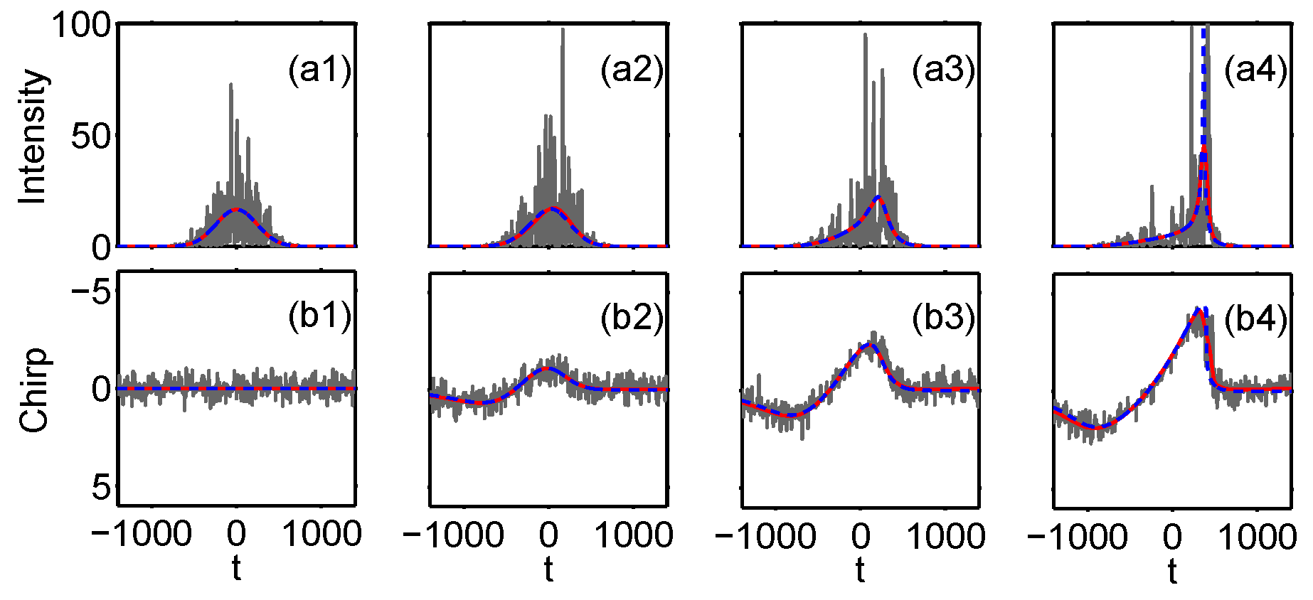
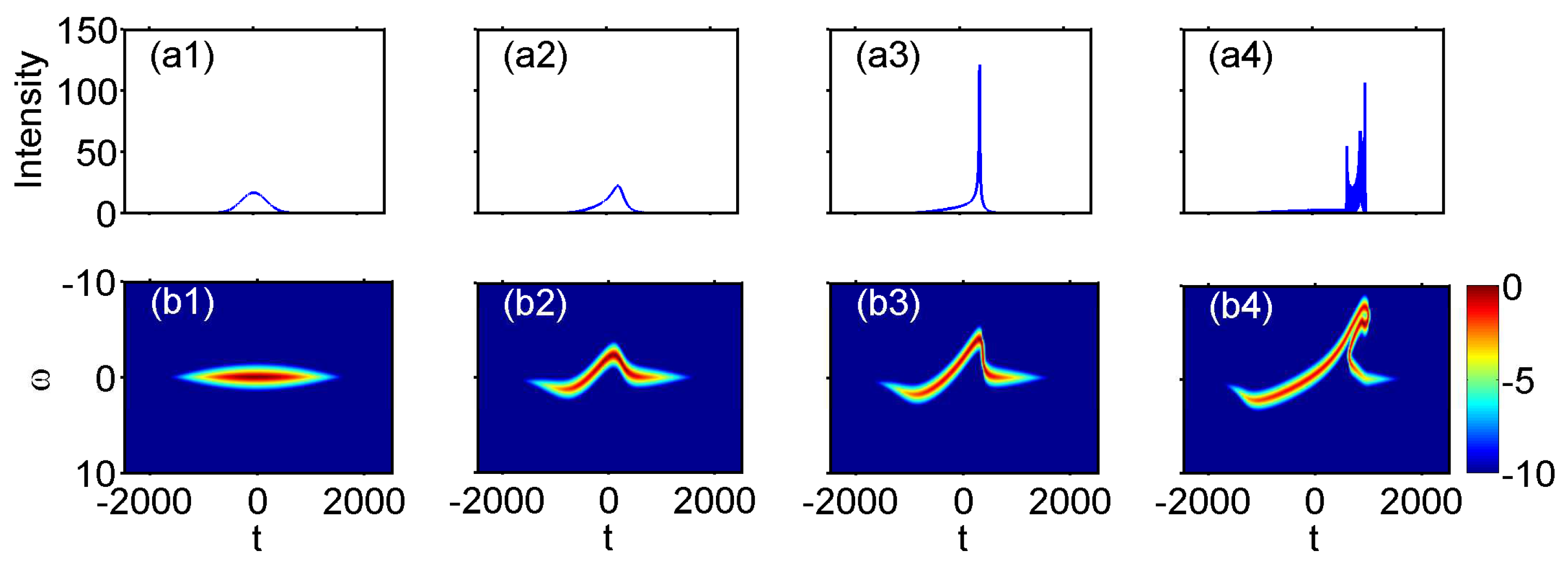
The situation is fundamentally different in the regime characterized by a highly non-instantaneous non-linear response time, . In contrast with the quasi-instantaneous non-linear regime, here the incoherent pulse exhibits a global collective behavior, in which it is the incoherent pulse as a whole that exhibits a shock singularity. This is illustrated in Figure 1, which shows the temporal dynamics of an initial incoherent pulse during its propagation through the non-linear medium, while the corresponding spectrogram dynamics is reported in Figure 2. The remarkable result is that, aside from the shock singularity revealed by the dynamics of the chirp, the global incoherent pulse also exhibits a dramatic narrowing and amplification as it is drifted in time. The subsequent analysis will reveal that this effect relies on the existence of a collapse singularity emanating from the envelope of the incoherent pulse. In this example we considered for simplicity an exponential-like response function, , where the prefactor is considered to ensure the continuity of the response function at the origin . This appears consistent with the variety of response functions considered for instance in [31] to model light propagation in liquid-filled PCFs.
3. Vlasov Approach
The collective incoherent behavior revealed by the NLS simulations can be described in detail by a temporal version of the long-range Vlasov formalism [28,38,39]. The Vlasov equation governs the evolution of the averaged spectrum of the incoherent wave , with the correlation function:
where is the temporal profile of the averaged intensity of the incoherent wave, and is the effective potential. Please note that since the statistics of the pulse is not stationary in time, the spectrum depends on the time position, i.e., it denotes the spectrogram of the optical pulse. The Vlasov Equation (2) conserves the total power . Contrary to the spatial case [28], in the temporal domain the potential is constrained by the causality of , which breaks the Hamiltonian structure of the Vlasov Equation (2) [28]. In the same way, the total momentum , is no longer conserved [40]. Please note that the Vlasov equation governs the evolution of the averaged spectrum , which is inherently a deterministic (smooth) function of the phase-space variables . In contrast, the NLS equation governs the evolution of an initial random function , which remains stochastic during the propagation in z. We compare the evolutions of the spectrograms of (e.g., Figure 2a) with the corresponding averaged spectra obtained from the numerical integration of the Vlasov equation e.g., Figure 2a)—we do not perform averages over the realizations of the initial random condition . We also note that in Figure 1 (as well as Figures 5 and 8) the direct comparison between the NLS and Vlasov simulations has been improved by smoothing the NLS data with an averaging over nearest-neighbor points (smooth MATLAB function).
4. Hydrodynamic-Like Model
4.1. Singular Solutions of the Vlasov Equation
The spectrogram dynamics can be described by means of singular solutions of the Vlasov equation [23,41], —note that the presence of the Dirac function reflects the narrowness of the spectrum evolving in the strongly non-linear regime. The function can be interpreted as a ‘momentum per particle’, a feature that becomes apparent by remarking that , where the momentum density is defined by . This leads to the following hydrodynamic-like model governing the evolutions of the intensity envelope , and momentum , of the incoherent pulse:
Starting from , the ‘spectrogram’ is initially driven by the last non-linear term in (4), while the Burgers-like (second) term of (4) subsequently leads to the gradient catastrophe of . The finite ‘time’ (distance, z) shock singularity of will be shown to be responsible for a collapse singularity of the intensity envelope .
4.2. Evolution Along the Characteristics
The singular behavior of the random wave can be described theoretically by solving Equations (3) and (4) by the method of the characteristics [42]. We define , , , and , which can be shown to satisfy the set of coupled ordinary differential equations (ODE):
where the dots denote the derivatives with respect to the evolution variable, . The method of the characteristics allows for a major simplification of the problem since the partial difference Equations (3) and (4) are reduced to a small number of ODEs (5)–(9) without approximations. A significant advantage of the ODEs (3) and (4) is that they show that the PDE system (5)–(9) exhibits finite ‘time’ singularities for the gradient of the momentum and the intensity. In addition, the ODEs (5)–(9) specify how such singularities develop during the time evolution of the system, see Equation (11) below.
The equations for the characteristics (5)–(9) look similar to those considered in the spatial domain for the propagation of two-dimensional speckle beams [23]. There is however an important difference with the spatial case: In the temporal case considered here, because of the causality condition inherent to the temporal response function, the derivatives of are not continuous at . This aspect becomes relevant by noting that the whole dynamics is driven by the gradient of the envelope of the incoherent pulse, i.e., the variable in Equation (8). In contrast with the spatial case, the effective potential and its derivatives are not uniformly bounded. As a consequence, the first source term in the equation for takes the general form . Considering the continuity of the response function () [43], we can write the evolution of the potential along the characteristic
The second term in the right-hand side is bounded (because is bounded and is constant). We anticipate that the first term is smaller than in Equation (8) (see Equation (11)), so that it cannot prevent from the catastrophic singularity. We then obtain the singular behaviors of and just before the singularity at :
Please note that the behavior of is obtained by remarking that, irrespective of the dispersion regime (normal or anomalous), we have from Equation (9) .
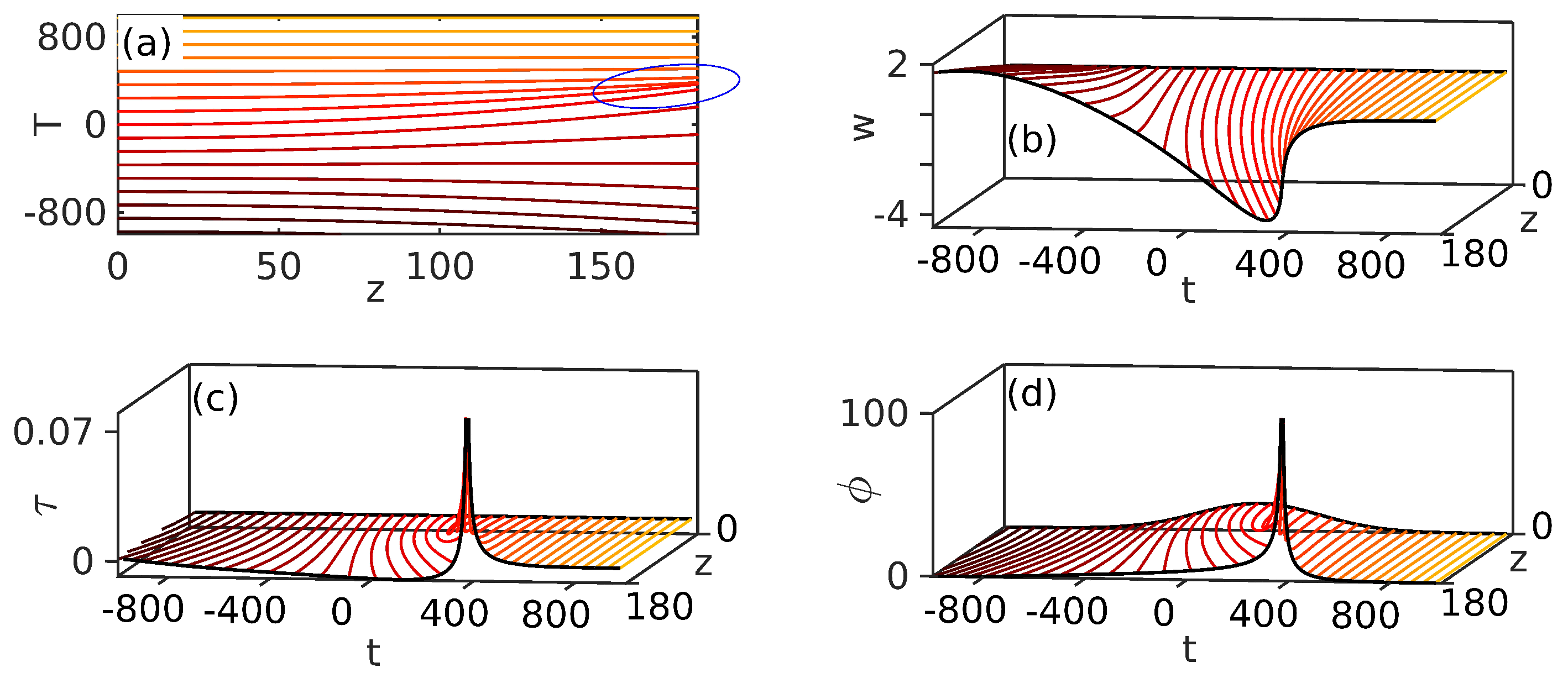
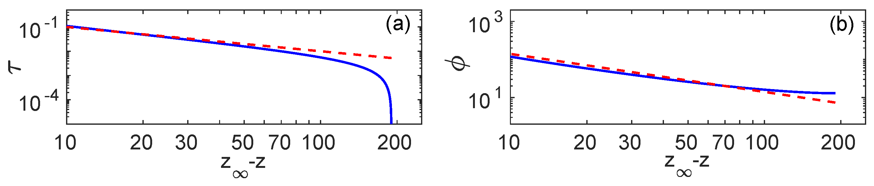
To complete our study we have solved by numerical integration the complete set of ODE (5)–(9)—note in this respect that the first term in the right-hand side of (7) involves partial derivatives of the effective potential taken along the characteristics , so that the numerical integration requires the explicit evolution of which is obtained by solving the hydrodynamic Equations (3) and (4). The evolutions of the characteristics are reported in Figure 3a for a set of initial conditions , which clearly show that the characteristics tend to approach each other nearby the shock point. Correspondingly, the evolution of the momentum of the incoherent pulse for such a set of initial conditions exhibit a self-steepening process followed by a shock singularity. Such a gradient catastrophe is reflected by the evolution of that exhibits a collapse singularity, which in turn induces a collapse singularity of the intensity envelope of the incoherent pulse . We have also verified that and exhibit a finite time singularity with the expected power-law divergence given by (11), as illustrated in Figure 4.
The analysis of the characteristic ODE (5)–(9) also reveals that, contrary to the (defocusing) spatial case where the response function is even and the field experiences two symmetric shock-singularities on the boundaries of the beam, in the temporal domain considered here the causality property of breaks the time symmetry , so that only one shock-collapse singularity is visible on the pulse evolution. According to Equations (8) and (10), the function is large for a characteristic where the intensity is itself large. Remarking that the intensity profile shifts toward , it turns out that a single shock-collapse singularity develops for , which inhibits the development of the singularity for . As a remarkable result, the initial incoherent pulse as a whole develops a temporal-asymmetric collapse singularity in the normal dispersion regime.
4.3. Dynamics after the Shock-Collapse Singularity
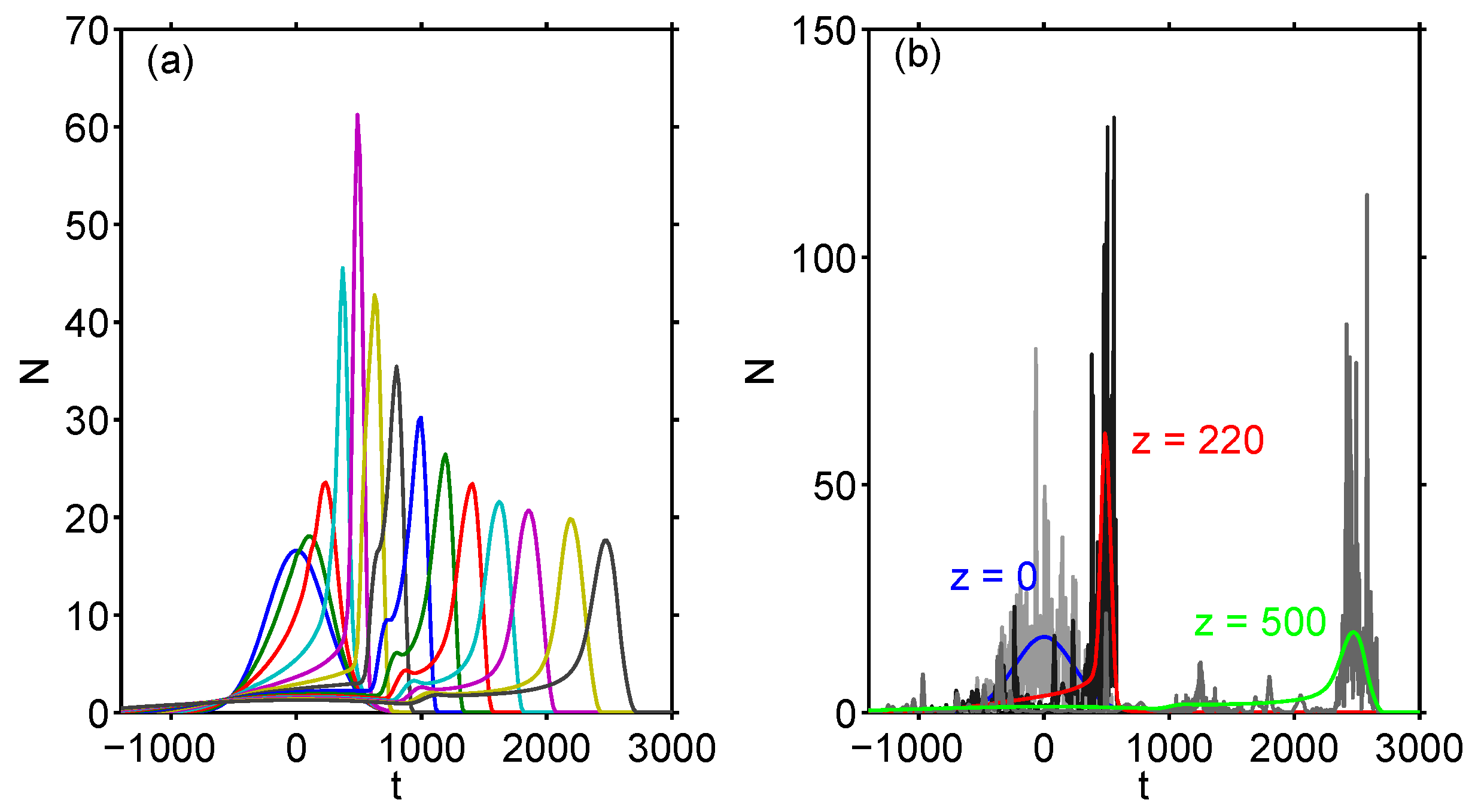
The hydrodynamic model (3) and (4) exhibits a finite ‘time’ singularity (11), which is regularized by the NLS and Vlasov equations (1) and (2)—note that the regularization is not characterized by the formation of rapid DSW oscillations. This is illustrated in Figure 5 and Figure 6 that show the evolution of the incoherent pulse after the shock-collapse singularity. The regularization becomes apparent by remarking that the spectrogram evolves in the two-dimensional phase-space so that its evolution can become ‘multi-valued’, as evidenced in Figure 6. This is in contrast with the function ruled by the hydrodynamic model (3) and (4) that undergoes the shock singularity and which is inherently a single valued function. The derivation of a more complete hydrodynamic-like model describing the regularization of the shock-collapse singularity is a difficult task related to a long-standing mathematical problem, namely achieving a closure of the infinite hierarchy of equations that govern the evolutions of -moments in transport kinetic equations [44,45]. It is important to note in this respect that the wave-turbulence closure is usually justified in the weakly non-linear regime [46,47,48,49] leading to the celebrated (Boltzmann-like) kinetic equation for optical waves [28], which describes important phenomena such as light thermalization [50,51,52,53,54,55], wave condensation [28], or the dynamics of certain fiber lasers [56,57,58,59]. On the other hand, the closure of moments equations considered here concerns the opposite strongly non-linear regime. This problem of regularization was discussed in [23] through the analysis of higher-order truncations of the hierarchy of moments equations. The analysis revealed that higher-order -moments become all of the same order of magnitude nearby the singularity (11), which prevents a closure of the hierarchy and thus a reduced description of the dynamics beyond the shock-collapse point.
5. Discussion and Conclusions
In summary, we have shown that a highly non-instantaneous non-linearity is responsible for a global collective behavior of an incoherent pulse, which is characterized by the development of the CSCS. The theoretical analysis is based on a long-range Vlasov formalism that exhibits interesting analogies with long-range gravitational systems [28,60,61]. The Vlasov equation has been reduced to a hydrodynamic model that has been solved by the method of the characteristics. The corresponding set of coupled ordinary differential equations provide a detailed description of the nature of the CSCS. This novel regime of incoherent wave propagation may shed new light on recent experiments of high-power incoherent supercontinuum generation in optical fibers [62]. More generally, we can envisage the experimental observation of the CSCS of incoherent waves owing to the recent progress made on the fabrication of PCF filled with liquids displaying highly non-instantaneous Kerr responses [30,31]. For example, in comparison to standard silica fibers, CS filled PCFs studied in the reference [34] exhibit interesting properties of the response function: The ratio between the instantaneous Kerr effect and the delayed Raman effect is 15:85, and in addition the response time can be as large as 1.5 ps. At the wavelength of 1550 nm, our preliminary numerical simulations indicate that if one injects incoherent pulses with a duration of 20 ps and a peak power of 1 KW, the incoherent shockwaves should be generated and observed after a propagation length of about 0.5 m in this kind of PCFs.
5.1. Toward Incoherent Rogue Waves?
We have seen that, as a consequence of the causality property of the response function, the intensity of the incoherent pulse exhibits a temporally drifted collapse behavior featured by a pronounced intensity peak. In a loose sense, this phenomenological behavior is reminiscent of a rogue-like wave phenomenon. Extreme wave events have been widely investigated in the context of optics [63,64,65,66], in particular in the presence of a non-instantaneous (Raman-like) non-linearity [67,68,69,70,71]. Note however that, although rogue waves have been shown to emerge from a turbulent environment, so far, the rogue wave itself has been always identified as being inherently a coherent localized entity [72,73,74,75,76,77,78,79,80,81,82,83,84]. In contrast, here, it is the incoherent pulse as a whole that leads to the formation of an extreme high-amplitude structure, a feature that may be interpreted in analogy with an incoherent rogue wave phenomenon. Work is in progress in order to study the spontaneous emergence of these collective incoherent events from an initial homogeneous random state of the field (i.e., with fluctuations that are statistically stationary in time).
5.2. Coherent Initial Conditions
We underline that the collapse-like behavior of the incoherent pulse originates in the highly non-instantaneous non-linearity. This can be seen by noting that in the limit of a (quasi-)instantaneous non-linearity () the hydrodynamic model Equations (3) and (4) recovers the shallow-water equations [1], which do not exhibit collapse singularities. In this respect, we note that the formation of the collapse singularity does not require an incoherent dynamic of the optical field. This is illustrated in Figure 7 that shows the evolution of the field by starting from a purely coherent initial pulse. As discussed in Refs. [14,15,85] in the spatial domain (non-local non-linearity), the evolution of the coherent field can be described by effective equations that are analogous to the hydrodynamic model (3) and (4), which precisely predicts the CSCS. Interestingly, the development of the shock singularity has been recently discussed in analogy with the quantum squeezing effect in phase-space [86], while its actual irreversible behavior has been discussed in relation to Gamow vectors [87]. Note in Figure 7 that, by starting from a coherent pulse, the post-collapse dynamics evidence the formation of an erratic dynamics of the field, as illustrated by NLS simulations in Figure 7. In its long term evolution, the incoherent field is expected to self-organize into an incoherent soliton [88], which would be sustained by the normal dispersion regime as discussed in Ref. [39,89].
5.3. Anomalous dispersion
We have focused the presentation of our work into the case where the incoherent pulse propagates in the normal dispersion regime. However, the analysis can easily be transposed to the anomalous dispersion regime (). As illustrated in Figure 8, the phenomenological behavior is very similar to the normal dispersion regime, except that the incoherent pulse develops the CSCS toward the negative temporal axis.
Author Contributions
A.P. and G.X. initialized the subject; J.G. and A.P. developed the theory; G.X. and A.F. performed the numerical simulations; A.P. supervised the project and wrote the paper. All the authors participated in the interpretations of the theoretical and numerical results.
Funding
This research was funded by the Labex ACTION (ANR-11-LABX-01-01) program.
Acknowledgments
The authors are grateful to S. Trillo and J. Barré for fruitful discussions.
Conflicts of Interest
The authors declare no conflict of interest.
References
- Whitham, G.B. Linear and Nonlinear Waves; Wiley: New York, NY, USA, 1974. [Google Scholar]
- El, G.A.; Hoefer, M.A. Dispersive shock waves and modulation theory. Physica D 2016, 333, 11–65. [Google Scholar] [CrossRef] [Green Version]
- Onorato, M.; Residori, S.; Baronio, F. (Eds.) Rogue and Shock Waves in Nonlinear Dispersive Media; Lectures Notes in Physics; Springer: Berlin, Germany, 2016. [Google Scholar]
- Taylor, R.J.; Baker, D.R.; Ikezi, H. Observation of collisionless electrostatic shocks. Phys. Rev. Lett. 1970, 24, 206–209. [Google Scholar] [CrossRef]
- Smyth, N.F.; Holloway, P.E. Hydraulic Jump and Undular Bore Formation on a Shelf Break. J. Phys. Oceanogr. 1988, 18, 947–962. [Google Scholar] [CrossRef] [Green Version]
- Rothenberg, J.E.; Grischkowsky, D. Observation of the formation of an optical intensity shock and wave breaking in the nonlinear propagation of pulses in optical fibers. Phys. Rev. Lett. 1989, 62, 531. [Google Scholar] [CrossRef]
- Wan, W.; Jia, S.; Fleischer, J.W. Dispersive superfluid-like shock waves in nonlinear optics. Nat. Phys. 2007, 3, 46–51. [Google Scholar] [CrossRef]
- Whalen, P.; Moloney, J.V.; Newell, A.C.; Newell, K.; Kolesik, M. Optical shock and blow-up of ultrashort pulses in transparent media. Phys. Rev. A 2012, 86, 033806. [Google Scholar] [CrossRef]
- Fatome, J.; Finot, C.; Millot, G.; Armaroli, A.; Trillo, S. Observation of Optical Undular Bores in Multiple Four-Wave Mixing. Phys. Rev. X 2014, 4, 021022. [Google Scholar] [CrossRef]
- Conforti, M.; Baronio, F.; Trillo, S. Resonant radiation shed by dispersive shock waves. Phys. Rev. A 2014, 89, 013807. [Google Scholar] [CrossRef]
- Wetzel, B.; Bongiovanni, D.; Kues, M.; Hu, Y.; Chen, Z.; Trillo, S.; Dudley, J.M.; Wabnitz, S.; Morandotti, R. Experimental Generation of Riemann Waves in Optics: A Route to Shock Wave Control. Phys. Rev. Lett. 2016, 117, 073902. [Google Scholar] [CrossRef] [Green Version]
- Trillo, S.; Deng, G.; Biondini, G.; Klein, M.; Clauss, G.F.; Chabchoub, A.; Onorato, M. Experimental Observation and Theoretical Description of Multisoliton Fission in Shallow Water. Phys. Rev. Lett. 2016, 117, 144102. [Google Scholar] [CrossRef] [Green Version]
- Xu, G.; Conforti, M.; Kudlinski, A.; Mussot, A.; Trillo, S. Dispersive Dam-Break Flow of a Photon Fluid. Phys. Rev. Lett. 2017, 118, 254101. [Google Scholar] [CrossRef] [PubMed]
- Ghofraniha, N.; Conti, C.; Ruocco, G.; Trillo, S. Shocks in Nonlocal Media. Phys. Rev. Lett. 2007, 99, 043903. [Google Scholar] [CrossRef] [PubMed]
- Ghofraniha, N.; Amato, L.S.; Folli, V.; Trillo, S.; DelRe, E.; Conti, C. Measurement of scaling laws for shock waves in thermal nonlocal media. Opt. Lett. 2012, 37, 2325–2327. [Google Scholar] [CrossRef] [PubMed]
- Karpov, M.; Congy, T.; Sivan, Y.; Fleurov, V.; Pavloff, N.; Bar-Ad, S. Spontaneously formed autofocusing caustics in a confined self-defocusing medium. Optica 2015, 2, 1053–1057. [Google Scholar] [CrossRef]
- El, G.A.; Smyth, N.F. Radiating dispersive shock waves in non-local optical media. Proc. R. Soc. A 2016, 472, 20150633. [Google Scholar] [CrossRef] [PubMed] [Green Version]
- Gentilini, S.; Braidotti, M.C.; Marcucci, G.; DelRe, E.; Conti, C. Nonlinear Gamow vectors, shock waves, and irreversibility in optically nonlocal media. Phys. Rev. A 2015, 92, 023801. [Google Scholar] [CrossRef]
- Fratalocchi, A.; Armaroli, A.; Trillo, S. Time-reversal focusing of an expanding soliton gas in disordered replicas. Phys. Rev. A 2011, 83, 053846. [Google Scholar] [CrossRef]
- Ghofraniha, N.; Gentilini, S.; Folli, V.; DelRe, E.; Conti, C. Shock waves in disordered media. Phys. Rev. Lett. 2012, 109, 243902. [Google Scholar] [CrossRef]
- Garnier, J.; Xu, G.; Trillo, S.; Picozzi, A. Incoherent Dispersive Shocks in the Spectral Evolution of Random Waves. Phys. Rev. Lett. 2013, 111, 113902. [Google Scholar] [CrossRef]
- Xu, G.; Garnier, J.; Trillo, S.; Picozzi, A. Impact of self-steepening on incoherent dispersive spectral shocks and collapse-like spectral singularities. Phys. Rev. A 2014, 90, 013828. [Google Scholar] [CrossRef]
- Xu, G.; Vocke, D.; Faccio, D.; Garnier, J.; Rogers, T.; Trillo, S.; Picozzi, A. From coherent shocklets to giant collective incoherent shock waves in nonlocal turbulent flows. Nat. Commun. 2015, 6, 8131. [Google Scholar] [CrossRef] [PubMed] [Green Version]
- Peccianti, M.; Conti, C.; Assanto, G.; de Luca, A.; Umeton, C. Routing of anisotropic spatial solitons and modulational instability in liquid crystals. Nature 2004, 2004 432, 733–737. [Google Scholar] [CrossRef]
- Krolikowski, W.; Bang, O.; Nikolov, N.I.; Neshev, D.; Wyller, J.; Rasmussen, J.J.; Edmundson, D. Modulational instability, solitons and beam propagation in spatially nonlocal nonlinear media. J. Opt. B Quant. Semicl. Opt. 2004, 6, S288. [Google Scholar] [CrossRef]
- Alberucci, A.; Jisha, C.P.; Smyth, N.F.; Assanto, G. Spatial optical solitons in highly nonlocal media. Phys. Rev. A 2015, 91, 013841. [Google Scholar] [CrossRef]
- Vocke, D.; Roger, T.; Marino, F.; Wright, E.M.; Carusotto, I.; Clerici, M.; Faccio, D. Experimental characterisation of nonlocal photon fluids. Optica 2015, 2, 484–490. [Google Scholar] [CrossRef]
- Picozzi, A.; Garnier, J.; Hansson, T.; Suret, P.; Randoux, S.; Millot, G.; Christodoulides, D. Optical wave turbulence: Toward a unified nonequilibrium thermodynamic formulation of statistical nonlinear optics. Phys. Rep. 2014, 542. [Google Scholar] [CrossRef]
- Fanjoux, G.; Michaud, J.; Maillotte, H.; Sylvestre, T. Slow-Light Spatial Solitons. Phys. Rev. Lett. 2008, 100, 013908. [Google Scholar] [CrossRef] [Green Version]
- Conti, C.; Schmidt, M.; Russell, P.; Biancalana, F. Highly noninstantaneous solitons in liquid-core photonic crystal fibers. Phys. Rev. Lett. 2010, 105, 263902. [Google Scholar] [CrossRef]
- Pricking, S.; Giessen, H. Generalized retarded response of nonlinear media and its influence on soliton dynamics. Opt. Express 2011, 19, 2895–2903. [Google Scholar] [CrossRef]
- Saleh, M.F.; Chang, W.; Hölzer, P.; Nazarkin, A.; Travers, J.C.; Joly, N.Y.; Russell, P.S.J.; Biancalana, F. Theory of photoionization-induced blueshift of ultrashort solitons in gas-filled hollow-core photonic crystal fibers. Phys. Rev. Lett. 2011, 107, 203902. [Google Scholar] [CrossRef]
- Husko, C.A.; Combrie, S.; Colman, P.; Zheng, J.; de Rossi, A.; Wong, C.W. Soliton dynamics in the multiphoton plasma regime. Sci. Rep. 2013, 3, 1100. [Google Scholar] [CrossRef]
- Chemnitz, M.; Gebhardt, M.; Gaida, C.; Stutzki, F.; Kobelke, J.; Limpert, J.; Tünnermann, A.; Schmidt, M.A. Hybrid soliton dynamics in liquid-core fibres. Nat. Commun. 2017, 8, 42. [Google Scholar] [CrossRef] [PubMed]
- Markos, C.; Travers, J.C.; Abdolvand, A.; Eggleton, B.J.; Bang, O. Hybrid photonic-crystal fiber. Rev. Mod. Phys. 2017, 89, 045003. [Google Scholar] [CrossRef]
- Saleh, M.F.; Armaroli, A.; Marini, A.; Biancalana, F. Strong Raman-induced noninstantaneous soliton interactions in gas-filled photonic crystal fibers. Opt. Lett. 2015, 40, 4058–4061. [Google Scholar] [CrossRef] [PubMed] [Green Version]
- Saleh, M.F.; Armaroli, A.; Tran, T.X.; Marini, A.; Belli, F.; Abdolvand, A.; Biancalana, F. Raman-induced temporal condensed matter physics in gas-filled photonic crystal fibers. Opt. Express 2015, 23, 11879–11886. [Google Scholar] [CrossRef] [PubMed]
- Kibler, B.; Michel, C.; Garnier, J.; Picozzi, A. Temporal dynamics of incoherent waves in noninstantaneous response nonlinear Kerr media. Opt. Lett. 2012, 37, 2472–2474. [Google Scholar] [CrossRef] [PubMed]
- Michel, C.; Kibler, B.; Garnier, J.; Picozzi, A. Temporal incoherent solitons supported by a defocusing nonlinearity with anomalous dispersion. Phys. Rev. A 2012, 86, 041801. [Google Scholar] [CrossRef]
- The wave-packet is red-shifted P(z) < 0 and evolves according to ∂zP(z) = ∫V(t,z)∂tN(t,z)dt, while the mean time position T(z) = ∫∫tnω(t,z)dtdω verifies ∂zT(z) = σP(z).
- Xu, G.; Garnier, J.; Faccio, D.; Trillo, S.; Picozzi, A. Incoherent shock waves in long-range optical turbulence. Physica D 2016, 333, 310–322. [Google Scholar] [CrossRef]
- Evans, L.C. Partial Differential Equations; AMS: Providence, RI, USA, 2002. [Google Scholar]
- If the response function is not continuous at the origin (0) ≠ 0 (e.g., purely exponential response), then ∂tN(T(z),z) could be of the same order as τ2(z) in Equation (8). However, at the time where N(t, z) is maximal, the term ∂tN(t, z) is zero, so that the system still exhibits the catastrophic singularity.
- Levermore, C.D. Moment closure hierarchies for kinetic theories. J. Stat. Phys. 1996, 83, 1021–1065. [Google Scholar] [CrossRef]
- Perin, M.; Chandre, C.; Morrison, P.J.; Tassi, E. Higher order Hamiltonian fluid reduction of Vlasov equation. Ann. Phys. 2014, 2014 348, 50–63. [Google Scholar] [CrossRef]
- Zakharov, V.E.; L’vov, V.S.; Falkovich, G. Kolmogorov Spectra of Turbulence I; Springer: Berlin, Germnay, 1992. [Google Scholar]
- Newell, A.C.; Rumpf, B. Wave Turbulence. Annu. Rev. Fluid Mech. 2011, 43, 59. [Google Scholar] [CrossRef]
- Newell, A.C.; Nazarenko, S.; Biven, L. Wave turbulence and intermittency. Physica D 2001, 152–153, 520. [Google Scholar] [CrossRef]
- Nazarenko, S. Wave Turbulence; Lectures Notes in Physics; Springer: Berlin, Germany, 2011. [Google Scholar]
- Barviau, B.; Kibler, B.; Picozzi, A. Wave-turbulence approach of supercontinuum generation: Influence of self-steepening and higher-order dispersion. Phys. Rev. A 2009, 79, 063840. [Google Scholar] [CrossRef]
- Laurie, J.; Bortolozzo, U.; Nazarenko, S.; Residori, S. Optical wave turbulence and the condensation of light. Phys. Rep. 2012, 514, 121. [Google Scholar] [CrossRef]
- Barviau, B.; Garnier, J.; Xu, G.; Kibler, B.; Millot, G.; Picozzi, A. Truncated thermalization of incoherent optical waves through supercontinuum generation in photonic crystal fibers. Phys. Rev. A 2013, 87, 035803. [Google Scholar] [CrossRef]
- Xu, G.; Garnier, J.; Rumpf, B.; Fusaro, A.; Suret, P.; Randoux, S.; Kudlinski, A.; Millot, G.; Picozzi, A. Origins of spectral broadening of incoherent waves: Catastrophic process of coherence degradation. Phys. Rev. A 2017, 96, 023817. [Google Scholar] [CrossRef]
- Guasoni, M.; Garnier, J.; Rumpf, B.; Sugny, D.; Fatome, J.; Amrani, F.; Millot, G.; Picozzi, A. Incoherent Fermi-Pasta-Ulam Recurrences and Unconstrained Thermalization Mediated by Strong Phase Correlations. Phys. Rev. X 2017, 7, 011025. [Google Scholar] [CrossRef]
- Santić, N.; Fusaro, A.; Salem, S.; Garnier, J.; Picozzi, A.; Kaiser, R. Nonequilibrium precondensation of classical waves in two dimensions propagating through atomic vapors. Phys. Rev. Lett. 2018, 120, 055301. [Google Scholar] [CrossRef]
- Babin, S.; Churkin, D.; Ismagulov, A.; Kablukov, S.; Podivilov, E. Four-wave-mixing-induced turbulent spectral broadening in a long Raman fiber laser. J. Opt. Soc. Am. B 2007, 24, 1729–1738. [Google Scholar] [CrossRef]
- Turitsyna, E.; Falkovich, G.; El-Taher, A.; Shu, X.; Harper, P.; Turitsyn, S. Optical turbulence and spectral condensate in long fibre lasers. Proc. R. Soc. A 2012, 468, 2496–2508. [Google Scholar] [CrossRef] [Green Version]
- Turitsyna, E.; Smirnov, S.; Sugavanam, S.; Tarasov, N.; Shu, X.; Babin, S.; Podivilov, E.; Churkin, D.; Falkovich, G.; Turitsyn, S. The laminar-turbulent transition in a fibre laser. Nat. Photon. 2013, 7, 783–786. [Google Scholar] [CrossRef]
- Churkin, D.; Kolokolov, I.; Podivilov, E.; Vatnik, I.; Vergeles, S.; Terekhov, I.; Lebedev, V.; Falkovich, G.; Nikulin, M.; Babin, S.; et al. Wave kinetics of a random fibre laser. Nat. Commun. 2015, 2, 6214. [Google Scholar] [CrossRef] [PubMed]
- Campa, A.; Dauxois, T.; Ruffo, S. Statistical mechanics and dynamics of solvable models with long-range interactions. Phys. Rep. 2009, 480, 57–159. [Google Scholar] [CrossRef] [Green Version]
- Levin, Y.; Pakter, R.; Rizzato, F.B.; Teles, T.N.; Benetti, F.P. Nonequilibrium statistical mechanics of systems with long-range interactions. Phys. Rep. 2014, 535, 1–60. [Google Scholar] [CrossRef] [Green Version]
- Heidt, A.M.; Feehan, J.S.; Price, J.H.V.; Feurer, T. Limits of coherent supercontinuum generation in normal dispersion fibers. J. Opt. Soc. Am. B 2017, 34, 764–775. [Google Scholar] [CrossRef]
- Akhmediev, N.; Pelinovsky, E. Introductory remarks on Discussion & Debate: Rogue Waves—Towards a Unifying Concept? Eur. Phys. J. Spec. Top. 2010, 185, 1–4. [Google Scholar]
- Onorato, M.; Residori, S.; Bortolozzo, U.; Montina, A.; Arecchi, F.T. Rogue Waves and Their Generating Mechanisms in Different Physical Contexts. Phys. Rep. 2013, 528, 47–89. [Google Scholar] [CrossRef]
- Dudley, J.M.; Dias, F.; Erkintalo, M.; Genty, G. Instabilities, breathers and rogue waves in optics. Nat. Photonics 2014, 8, 755–764. [Google Scholar] [CrossRef] [Green Version]
- Akhmediev, N.; Kibler, B.; Baronio, F.; Belic, M.; Zhong, W.; Zhang, Y.; Chang, W.; Soto-Crespo, J.-M.; Vouzas, P.; Grelu, P.; et al. Roadmap on optical rogue waves and extreme events. J. Opt. 2016, 18, 063001. [Google Scholar] [CrossRef] [Green Version]
- Hammani, K.; Picozzi, A.; Finot, C. Extreme statistics in Raman fiber amplifiers: From analytical description to experiments. Opt. Commun. 2011, 284, 2594–2603. [Google Scholar] [CrossRef] [Green Version]
- Monfared, Y.E.; Ponomarenko, S.A. Non-Gaussian statistics and optical rogue waves in stimulated Raman scattering. Opt. Express 2017, 2017 25, 5941–5950. [Google Scholar] [CrossRef]
- Monfared, Y.E.; Ponomarenko, S.A. Non-Gaussian statistics of extreme events in stimulated Raman scattering: The role of coherent memory and source noise. Phys. Rev. A 2017, 96, 043817. [Google Scholar] [CrossRef]
- Chen, S.; Baronio, F.; Soto-Crespo, J.M.; Grelu, P.; Conforti, M.; Wabnitz, S. Optical rogue waves in parametric three-wave mixing and coherent stimulated scattering. Phys. Rev. A 2015, 92, 033847. [Google Scholar] [CrossRef]
- Armaroli, A.; Conti, C.; Biancalana, F. Rogue solitons in optical fibers: A dynamical process in a complex energy landscape? Optica 2015, 2, 497–504. [Google Scholar] [CrossRef]
- Akhmediev, N.; Ankiewicz, A.; Soto-Crespo, J.M. Rogue waves and rational solutions of the nonlinear Schrödinger equation. Phys. Rev. E 2009, 80, 026601. [Google Scholar] [CrossRef] [PubMed]
- Hammani, K.; Kibler, B.; Finot, C.; Picozzi, A. Emergence of rogue waves from optical turbulence. Phys. Lett. A 2010, 374, 3585–3589. [Google Scholar] [CrossRef]
- Kibler, B.; Hammani, K.; Finot, C.; Picozzi, A. Rogue waves, rational solitons and wave turbulence theory. Phys. Lett. A 2011, 3149–3155. [Google Scholar] [CrossRef]
- Walczak, P.; Randoux, S.; Suret, P. Optical Rogue Waves in Integrable Turbulence. Phys. Rev. Lett. 2015, 114, 143903. [Google Scholar] [CrossRef]
- Suret, P.; el Koussaifi, R.; Tikan, A.; Evain, C.; Randoux, S.; Szwaj, C.; Bielawski, S. Single-shot observation of optical rogue waves in integrable turbulence using time microscopy. Nat. Commun. 2016, 7, 13136. [Google Scholar] [CrossRef] [Green Version]
- Agafontsev, D.S.; Zakharov, V.E. Integrable turbulence and formation of rogue waves. Nonlinearity 2015, 2015 28, 2791–2821. [Google Scholar] [CrossRef]
- Soto-Crespo, J.M.; Devine, N.; Akhmediev, N. Integrable Turbulence and Rogue Waves: Breathers or Solitons? Phys. Rev. Lett. 2016, 116, 103901. [Google Scholar] [CrossRef] [PubMed]
- Akhmediev, N.; Soto-Crespo, J.M.; Devine, N. Breather turbulence versus soliton turbulence: Rogue waves, probability density functions, and spectral features. Phys. Rev. E 2016, 94, 022212. [Google Scholar] [CrossRef] [PubMed]
- Safari, A.; Fickler, R.; Padgett, M.J.; Boyd, R.W. Generation of Caustics and Rogue Waves from Nonlinear Instability. Phys. Rev. Lett. 2017, 119, 203901. [Google Scholar] [CrossRef] [PubMed]
- Toffoli, A.; Proment, D.; Salman, H.; Monbaliu, J.; Frascoli, F.; Dafilis, M.; Stramignoni, E.; Forza, R.; Manfrin, M.; Onorato, M. Wind generated rogue waves in an annular wave flume. Phys. Rev. Lett. 2017, 118, 144503. [Google Scholar] [CrossRef] [PubMed]
- Tikan, A.; Bielawski, S.; Szwaj, C.; Randoux, S.; Suret, P. Single-shot measurement of phase and amplitude by using a heterodyne time-lens system and ultrafast digital time-holography. Nat. Photon. 2018, 2018 12, 228–234. [Google Scholar] [CrossRef]
- el Koussaifi, R.; Tikan, A.; Toffoli, A.; Randoux, S.; Suret, P.; Onorato, M. Spontaneous emergence of rogue waves in partially coherent waves: A quantitative experimental comparison between hydrodynamics and optics. Phys. Rev. E 2018, 97, 012208. [Google Scholar] [CrossRef] [Green Version]
- Wang, J.; Ma, Q.W.; Yan, S.; Chabchoub, A. Breather rogue waves in random seas. Phys. Rev. Appl. 2018, 9, 014016. [Google Scholar] [CrossRef]
- Fusaro, A.; Garnier, J.; Xu, G.; Conti, C.; Faccio, D.; Trillo, S.; Picozzi, A. Emergence of long-range phase coherence in nonlocal fluids of light. Phys. Rev. A 2017, 95, 063818. [Google Scholar] [CrossRef]
- Braidotti, M.C.; Mecozzi, A.; Conti, C. Squeezing in a nonlocal photon fluid. Phys. Rev. A 2017, 96, 043823. [Google Scholar] [CrossRef]
- Marcucci, G.; Braidotti, M.C.; Gentilini, S.; Conti, C. Time asymmetric quantum mechanics and shock waves: exploring the irreversibility in nonlinear optics. Ann. Phys. 2017, 529, 1600349. [Google Scholar] [CrossRef]
- Picozzi, A.; Garnier, J. Incoherent soliton turbulence in nonlocal nonlinear media. Phys. Rev. Lett. 2011, 107, 233901. [Google Scholar] [CrossRef] [PubMed]
- Xu, G.; Garnier, J.; Picozzi, A. Spectral long-range interaction of temporal incoherent solitons. Opt. Lett. 2014, 39, 590–593. [Google Scholar] [CrossRef] [PubMed]
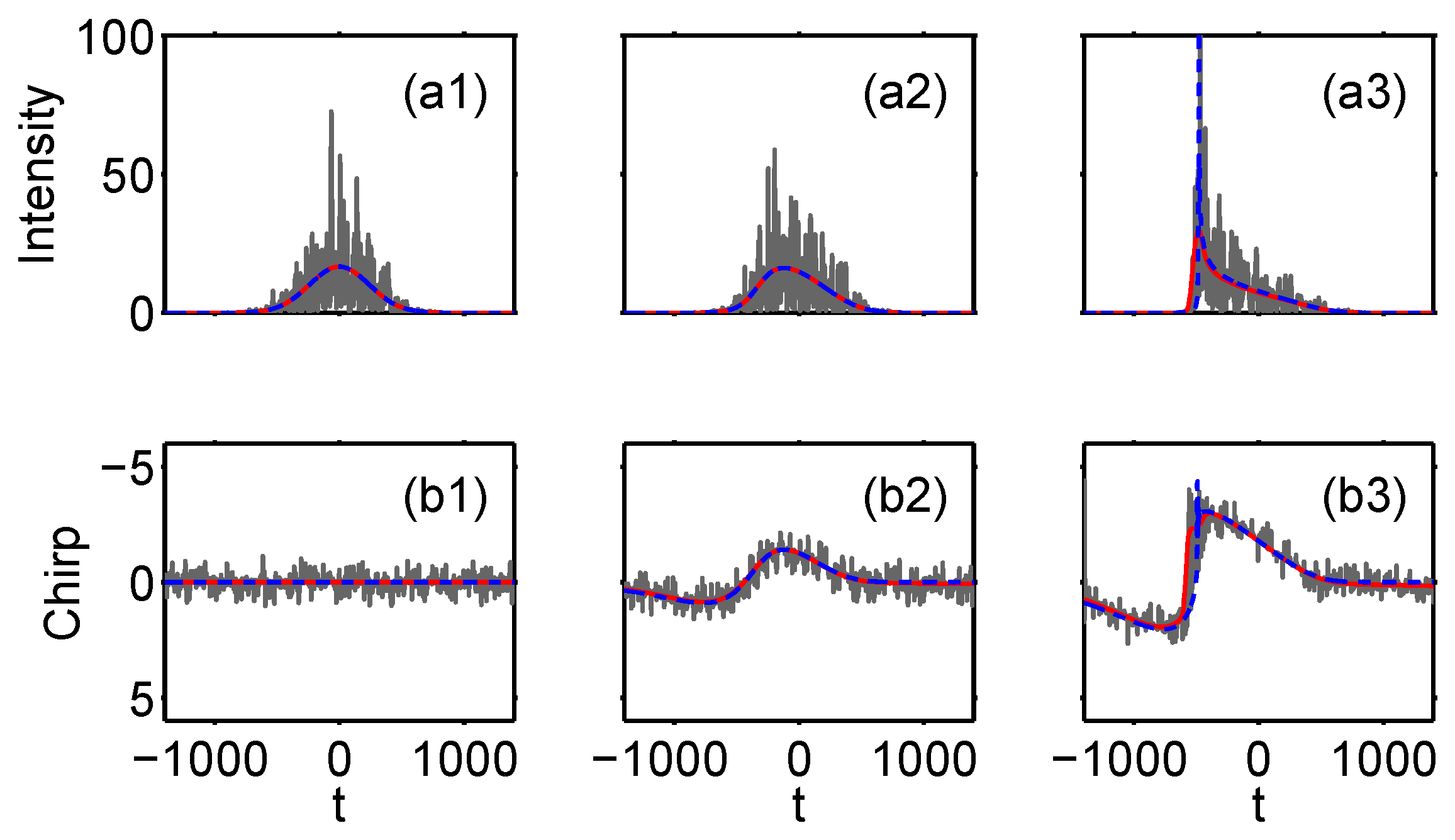
Figure 1.
Numerical simulations of the NLS Equation (1) (gray line), of the Vlasov Equation (2) (red line), and of the hydrodynamic-like Equation (3) and (4) (blue line). (a) Evolution of the intensity of the field that develops a collapse singularity, and corresponding evolution of the momentum (chirp) that develops a shock singularity (b). The quantitative agreement between the different models is obtained without using adjustable parameters. Propagation lengths at from left to right, , .

Figure 2.
Phase-space representation of the shock-collapse singularity shown in Figure 1: (a) Numerical simulation of the NLS Equation (1) showing the evolution of the spectrogram. (b) Numerical simulation of the Vlasov Equation (2). Propagation lengths at from left to right, , .

Figure 3.
Numerical integration of the coupled system of characteristic ODE (5)–(9): (a) Characteristics for a set of initial conditions . Corresponding evolutions of the momentum (chirp) (b) that exhibits a shock singularity, i.e., a collapse singularity for the corresponding gradient (c), which in turn induces a collapse singularity for the envelope of the incoherent pulse (d) ().

Figure 4.
Numerical integration of the coupled system of characteristic ODE (5)–(9): Evolutions during the propagation of the gradient of the momentum (a) and intensity envelope of the incoherent pulse (b) along a characteristic nearby the singularity. Their evolutions exhibit the power-law divergence predicted by the theory in Equation (11) (dashed red lines) ().

Figure 5.
(a) Post-collapse dynamics: Numerical simulation of the Vlasov Equation (2) showing the evolution of the intensity of the incoherent pulse at the propagation lengths , : The collapse-like behavior at is regularized as evidenced by the saturation and subsequent relaxation of the amplitude of the incoherent pulse (). (b) Comparison of the simulations of the NLS equation (1) (light gray, black, dark gray), and of the Vlasov Equation (2) at (blue), (red) nearby the shock-collapse point, (green)—the agreement between the NLS and Vlasov simulations is obtained without adjustable parameters.

Figure 6.
Phase-space representation of the post-shock-collapse singularity shown in Figure 2: (a) Numerical simulation of the NLS Equation (1) showing the evolution of the spectrogram. (b) Numerical simulation of the Vlasov Equation (2) showing the evolution of . The agreement between the NLS and Vlasov simulations is obtained without adjustable parameters. Parameters are: , , with the propagation lengths from left to right.

Figure 7.
Coherent dynamics: Numerical simulation of the NLS Equation (1) showing the evolution of the intensity (a), and corresponding spectrogram (b), with the same parameters as in Figure 1 and Figure 2, except that the initial condition is a fully coherent pulse. The coherent field exhibits a shock-collapse singularity and develops an incoherent behavior after the singularity. The corresponding propagation distances are from left to right.

Figure 8.
Anomalous dispersion regime: Numerical simulations of the NLS equation (1) (gray line), of the Vlasov Equation (2) (red line), and of the hydrodynamic-like Equations (3) and (4) (blue line). In analogy with the normal dispersion regime (Figure 1), the evolution of the intensity of the field develops a collapse singularity (a), while the momentum (chirp) develops a shock singularity (b). The good agreement between the different models is obtained without using adjustable parameters. Parameters are: , , with the propagation lengths from left to right.

© 2018 by the authors. Licensee MDPI, Basel, Switzerland. This article is an open access article distributed under the terms and conditions of the Creative Commons Attribution (CC BY) license (http://creativecommons.org/licenses/by/4.0/).
Share and Cite
MDPI and ACS Style
Xu, G.; Fusaro, A.; Garnier, J.; Picozzi, A. Incoherent Shock and Collapse Singularities in Non-Instantaneous Nonlinear Media. Appl. Sci. 2018, 8, 2559. https://0-doi-org.brum.beds.ac.uk/10.3390/app8122559
AMA Style
Xu G, Fusaro A, Garnier J, Picozzi A. Incoherent Shock and Collapse Singularities in Non-Instantaneous Nonlinear Media. Applied Sciences. 2018; 8(12):2559. https://0-doi-org.brum.beds.ac.uk/10.3390/app8122559
Chicago/Turabian StyleXu, Gang, Adrien Fusaro, Josselin Garnier, and Antonio Picozzi. 2018. "Incoherent Shock and Collapse Singularities in Non-Instantaneous Nonlinear Media" Applied Sciences 8, no. 12: 2559. https://0-doi-org.brum.beds.ac.uk/10.3390/app8122559
Note that from the first issue of 2016, this journal uses article numbers instead of page numbers. See further details here.