Multi-Objective Stochastic Optimal Operation of a Grid-Connected Microgrid Considering an Energy Storage System

1
Institute of Electrical Engineering, Shanghai University of Electric Power, Shanghai 200090, China
2
Key Laboratory of Control of Power Transmission and Conversion, Shanghai Jiao Tong University, Shanghai 200240, China
*
Author to whom correspondence should be addressed.
Appl. Sci. 2018, 8(12), 2560; https://0-doi-org.brum.beds.ac.uk/10.3390/app8122560
Submission received: 28 October 2018
/
Revised: 6 December 2018
/
Accepted: 7 December 2018
/
Published: 10 December 2018
(This article belongs to the Section Energy Science and Technology)
Abstract
:This paper investigates the stochastic optimal operation of microgrid considering the influence of energy storage system (ESS). The uncertain factors related to renewable energies are also fully considered. Monte Carlo simulation (MCS) and scenario reduction technique are used to capture the randomness of renewable energy output. The objective is to minimize the operation cost and pollutant treatment cost of the microgrid system. Then, the multi-objective optimization problem is transformed to a single-objective problem by a line weighted sum method. A nonlinear programming tool—General Algebraic Modeling System (GAMS)—is adopted to solve the single-objective problem. Simulation results indicate that the total cost of the microgrid system can be reduced effectively when considering the effect of ESS and verify the correctness of the proposed strategy.
1. Introduction
Microgrids have played an important role in solving the global energy crisis issue and, in recent years, microgrids have received more and more attention [1,2]. According to the definition by the U.S. Department of Energy, a microgrid is “a group of interconnected loads and Distributed Energy Resources within clearly defined electrical boundaries, which is considered as a single controllable entity from the main grid point of view [3]”. A microgrid can either work in grid-connected mode or stand-alone mode. The microgrid is extremely appealing owing to its flexibility, economy, and environmental protection.
In [4], an optimal energy planning of a stand-alone microgrid considering system uncertainties is studied to evaluate the system performance. In [5,6], several real-time optimization and energy management approaches considering ESS lifetime are proposed for an isolated microgrid. A multi-layer ant colony algorithm is adopted to address the problem. In [7], a novel expert fuzzy system—a grey wolf optimization based intelligent meta-heuristic method for battery sizing and energy management—is proposed. In [8], a fuzzy multi-objective optimization model with corresponding constraints to minimize the economic cost and network loss of microgrid is presented. In [9], the optimal operation problem is decomposed into two sub-problems of unit combination and optimal power flow. Ref. [10] discusses the optimal scheduling problem of accessible energies for a stand-alone microgrid. Ref. [11] presents a model-based method to analyze the performance of a domestic photovoltaic power plant with ESS. Among the research, the operation strategy optimization is limited to stand-alone microgrid. However, once the load demand of the microgrid changes significantly, the system may not be able to meet the load demand and loses stability as a result.
Ref. [12] investigates the coordinated optimal dispatch of ESSs to minimize the electricity costs in a group of grid-connected microgrids. In [13], a dynamic optimal operation atrategy for a microgrid in both stand-alone and grid-connected mode is presented. Dynamic programming (DP) and equal incremental fuel cost method are employed to solve the problem. In [14], a central controller based on mixed-integer-linear programming (MILP) is proposed to solve the optimal dispatch problem of a stand-alone microgrid. In the above research, the operation models are all built on deterministic optimization. The predictive errors of renewable energies are ignored. However, the uncertainty of renewable energies has a great influence on the safe and economical operation of microgrid. A modeling method which integrates both the deterministic and the stochastic nature of renewable power plants using a novel methodology inspired from reliability engineering: the Stochastic Hybrid Fault Tree Automaton is proposed in [15]. A novel probabilistic optimization model considering random characteristics of renewables and load profile is developed in [16]. Chance constraint programming for bi-objective optimal scheduling is used to solve the problem. In [17,18], MCS and Roulette mechanism are utilized to generate scenarios and a backward scenario reduction technique is applied to simplify the problem and reduce the computational burden.
In [19], a multi-objective optimal dispatch model for a grid-connected microgrid is raised. The optimization model is solved by an improved Particle Swarm Optimization (PSO) algorithm. In [20], a distributed control method based on multi-agent is proposed, which is used to deal with the complex energy management problems in the microgrid and multi-agent coordination is realized by game theory. Ref. [21] proposes an optimization strategy to provide the required energy for the microgrid system. PSO and Gaussian mutation algorithm are used to solve this problem. The above heuristic algorithms are sensitive to initial guesses that they can hardly find the global optimal solution. In [22], an advanced dynamic programming approach for energy management problem is presented by MATLAB (MATLAB 5.3(R11), MathWorks, Natick, MA, USA) and GAMS/Cplex 12 software, which is a numerical algorithm with good convergence characteristics.
Compared with the research mentioned above, the major contributions of this paper can be generalized as follows: (1) a multi-objective optimization model of a microgrid under a grid-connected mode is proposed; (2) a stochastic framework based on MCS and a scenario reduction method is proposed to deal with the uncertainties of renewable energy generation; (3) GAMS is utilized to solve the optimization model to find the global optimal solution; and (4) the influence of ESS on the optimization result of the microgrid are fully investigated.
The rest of this paper is arranged as follows. Firstly, the modeling of microgrid components is described in Section 2. The uncertainty modeling of renewable energies is analyzed in Section 3. The multi-objective optimization model of the microgrid system is described in Section 4, while the case study is given in Section 5. Finally, Section 6 gives conclusions and perspectives.
2. Modeling of Microgrid
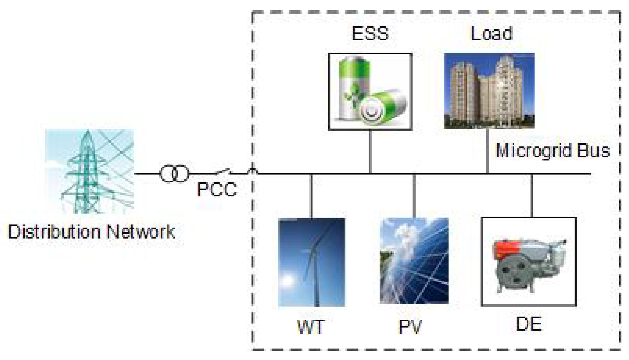
The microgrid system studied in this paper contains wind turbines (WT), photovoltaic (PV), diesel engine (DE), energy storage system (ESS) and load. The structure of the microgrid is shown in Figure 1.
2.1. Modeling of WT
The output power of WT depends on the wind speed to a large extent, which can be described as follows [23]:
where is the actual output power of WT, kW; v is the actual wind speed, m/s; is the rated power of WT, kW; is the cut-in wind speed, m/s; is the rated wind speed, m/s; and is the cut-out wind speed, m/s.
2.2. Modeling of PV
For the convenience of engineering research, it is generally believed that the output power of PV is only related to solar radiation and environmental temperature, which can be described as follows [24]:
where is the actual output power of PV, kW; is the maximum output power of PV under standard test conditions (STC), kW; is the actual irradiation received by PV; is the irradiation received by PV under STC, i.e., 1000 W/m; is the power generation temperature coefficient of PV; is the actual temperature of PV cells; is the rated temperature of PV cells, i.e., 25 C.
2.3. Modeling of DE
DE, as an important controllable unit in the microgrid, can be flexibly regulated. The fuel cost of DE can be described as:
where is the output power of DE, kW; are the fuel cost coefficients of DE.
2.4. Modeling of Energy Storage System
The lead-acid batteries are adopted as ESS in the microgrid studied in this paper. Compared with other energy storage technologies, the lead-acid batteries have higher charging efficiency and energy density and it is not constrained by space, so it is a better choice. The model of lead-acid can be expressed as [25]:
where is the state of charge(SOC) value of ESS at time t; are the charging and discharging power of ESS, respectively, kW; is the charging efficiency of ESS, which is set as 0.9 in this paper; is the discharging efficiency of ESS, which is set as 0.9 in this paper; is the capacity of ESS, kWh.
3. Uncertainty Modeling of WT/PV
The output power of WT and PV are greatly affected by weather conditions such as wind speed, solar radiation and environment temperature. In order to make the optimization result more accurate, the microgrid optimization model should take the influence of uncertain factors into consideration.
In order to consider the predictive error of renewable energies, the scenario-based representation is used [26]. In this case, a scenario is a sequence of hourly output power values of WT and PV. In this paper, the MCS method is adopted to generate multiple scenarios that represent these uncertain parameters based on the corresponding probability distribution functions [27,28]. Forecast values of wind speed, solar radiation and temperature of the next day should be obtained in order to generate scenarios. It is assumed that the wind speed, solar radiation intensity and temperature prediction error obey normal distribution with mean value and variance , where the values of and can be calculated from historical data. The probability density function of the forecast error is:
The final forecast value can be calculated by Equation (6):
where is the original forecast value.
It is worth noting that, in this paper, we suppose that the uncertainties related to WT and PV are independent [28]. Although increasing the number of scenarios can make the accuracy of the model better, a large number of scenarios will hinder the establishment of the model in the stochastic optimization method. Therefore, a suitable scenario reduction technique must be used to reduce the number of available scenarios to a representative set. The backward scenario reduction technique [26] is utilized in this study.
4. Problem Formulation
4.1. Microgrid without Access to ESS
When the microgrid has no access to ESS, the load demand of the system is provided by WT, PV, and DE together with the main grid. The objective function can be described as follows:
where S is the total number of scenarios; T is the total number of time intervals; s is the scenario index; t is the time index; is the probability of scenario s; are the generating cost of WT, PV respectively; is the generating cost of DE; is the transaction cost with main grid; is the generation cost coefficient of WT, yuan/kW; is the generation cost coefficient of PV, yuan/kW; is electricity price during time period t, yuan/kW; is the operation and maintenance cost coefficient of DE, yuan/kW; J is the total number of pollutant types, including , and ; is the treatment cost of the pollutant, yuan/kg; is the pollutant emission factor of DE, g/kW; is the pollutant emission factor of the main grid, g/kW.
The following constraints should be satisfied:
where is load demand of the microgrid, kW; is the minimum output power of DE, kW; is the maximum output power of DE, kW; is the maximum ramp up rate, kW/h; is the maximum ramp down rate, kW/h; is the maximum exchange power between the microgrid and main grid, kW.
4.2. Microgrid with ESS
ESS is one of the important components of the WT/PV/DE/ESS microgrid. The operation strategy of ESS has a great impact on the economic operation of the microgrid. When the load demand of the microgrid system is small or the electricity prices are low, the ESS operates in the charging mode. When the load demand is high or the electricity prices are expensive, the ESS operates in the discharging mode. Additionally, ESS can smooth the fluctuation of wind speed and solar radiation and enhance the load availability [29,30]. When the microgrid has access to ESS, the operation cost can be expressed as:
where is the operation cost of ESS; is the operation and maintenance cost coefficient of ESS, yuan/kW; is the charging power of ESS, kW; is the discharging power of ESS, kW.
The model of pollutant treatment cost is the same as Formula (6). The microgrid system should satisfy the following constraints:
where is the maximum charging power of ESS, kW; is the maximum discharging power of ESS, kW; equals 1 if the battery is charging during period t and 0, otherwise; equals 1 if the battery is discharging during period t and 0, otherwise; is the minimum SOC of ESS; is the maximum SOC of ESS; is the SOC of ESS at the end of the day; is the SOC of ESS at the beginning of the day.
The total power generation of WT, PV, DE, ESS and the main grid must be equal to the total load demand of the microgrid system at any time, which is constrained by Formula (19). For ESS, constraints (20) and (21) are the maximum charging/discharging power limits. These two states are mutually exclusive, which is ensured by Formula (22). The state of charge (SOC) of ESS is defined in Formula (4) and the SOC of ESS is limited by Formula (25). Furthermore, Formulas (14)–(16) should be satisfied as well.
4.3. Solution Method
The objective function of the optimization model is to minimize the operation cost (F1) and the pollutant treatment cost (F2). Therefore, the linear weighted sum method is adopted to transform the multi-objective optimization problem into a single-objective optimization problem. The final optimization model can be expressed as:
where are weight coefficient, which are set as 0.5 and 0.5, respectively, in this paper.
GAMS is a high-level modeling system for mathematical programming and optimization. It consists of a language compiler and a stable of integrated high-performance solvers. GAMS is tailored for complex, large scale modeling applications, and allows users to build large maintainable models that can be adapted quickly to new situations. GAMS is specifically designed for modeling linear, nonlinear and mixed integer optimization problems. Due to these advantages, GAMS is a suitable software to solve the problem proposed in this paper.
5. Case Study
5.1. System Configuration
The experimental microgrid is shown in Figure 1. Parameters of various microsources [31] are listed in Table 1. The WT and PV generation forecast data are obtained from a generation site in Shanghai as shown in Figure 2. The load forecast data are obtained from a residential building in Yangpu district, which is shown in Figure 3. Since the load prediction accuracy is up to 95% [32], this paper assumes that the actual load value is equal to the predictive value in order to simplify the model. The forecast errors of wind power and PV output power are assumed to be independent normal distribution with 35% standard deviation. The ESS data are scaled from a lead-acid battery system project in China [33] as shown in Table 2. The environmental parameters of DE and main grid are listed in Table 3 [34]. The time-of-use (TOU) electricity price of Shanghai, China is adopted and shown in Figure 4 [31].
5.2. Results and Discussion
5.2.1. Case 1: Optimization Results without ESS
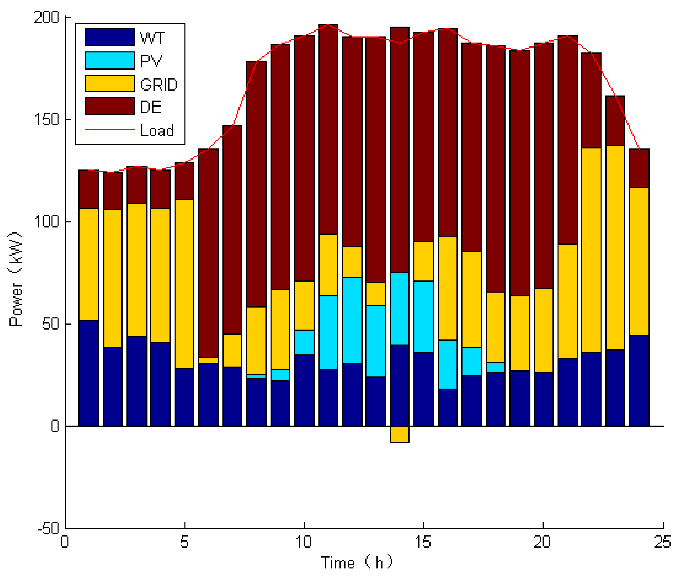
Figure 5 shows the optimal power flow of the microgrid without access to ESS in a daily basis.
It can be observed from the simulation result that the main grid plays an important role in providing power for load during the valley-price periods. While during peak-price periods, most of the load demand is satisfied by DE instead of by purchasing electricity from the main grid. During flat-price periods, the load demand of microgrid is satisfied by both DE and the distribution network, but DE output accounts for a larger proportion relatively.
5.2.2. Case 2: Optimization Results with ESS
In this case, ESS is added to the available generation units to enhance the flexibility of the energy production department. The optimal power flow considering ESS is shown in Figure 6. The charging and discharging power of ESS is shown in Figure 7.
It can be concluded from Figure 6 that the output power of DE in this case is the same as that in Case 1. The participation of ESS helps explain the increase of the power exchanged with the main grid (both purchasing and selling). The microgrid purchases energy from the main grid and stores the excess energy in the ESS when the electricity prices are low. Conversely, the ESS releases the stored power to reduce the power purchased from the main grid in order to reduce the operation cost when the electricity prices are high.
In addition, Figure 8 shows the SOC of the ESS. In order to extend the battery life, the SOC is always between 25% and 95%.
When 1 = 2 = 0.5, the financial results are listed in Table 4.
It can be seen from Table 4 that the total cost of the microgrid system in Case 2 is lower than that in Case 1 when the microgrid has no access to ESS, indicating that the ESS discharges to supply partial load at peak load times and peak price times from 8:00 a.m. to 10:00 a.m., 12:00 p.m. to 1:00 p.m. and 6:00 p.m. to 8:00 p.m., which is conductive to decreasing the total cost of the microgrid. The pollutant treatment cost in Case 1 is higher than that in Case 2, which is attributed to the fact that the pollutant treatment cost of the main grid is higher compared to DE. It is calculated that, when the microgrid has access to ESS, the total cost is reduced by 2.67% and the operating cost by 4.14%, although the pollutant treatment cost is increased by 1.02%. Therefore, in general, Case 2 is preferable to Case 1.
6. Conclusions
This paper developed a stochastic multi-objective framework for the optimal operation of a grid-connected microgrid with ESS. The main contributions and the conclusions of this paper are summarized as follows:
(1) In order to implement more precise modeling, Monte Carlo simulation and backward scenario reduction technique were employed to simulate the stochastic characteristic of the solar radiation and wind speed.
(2) A multi-objective optimization model for microgrid is proposed to minimize both the operational cost and pollutant treatment cost of the microgrid system.
(3) The proposed multi-objective optimization model was transformed to a single-objective model by a linear weighted sum method. In addition, GAMS was employed to solve the problem in order to find the global optimal solution.
(4) The results show that the presence of ESS can reduce the total cost effectively. The total cost is 2328.4163 yuan in Case 1 and 2266.3451 yuan in Case 2, which brings 2.67% cost savings for the entire system in a daily basis.
The disadvantage of this paper is that the reliability index of the microgrid system is not fully considered, which should be investigated in the future research.
Author Contributions
The author H.F. conceived and designed the article; Q.Y. carried out the main research tasks and wrote the full manuscript and performed the experiment; H.C. analyzed the results and the whole manuscript.
Funding
This research was funded by [National Key Research and Development Program] grant numder [2016YFB0900100].
Acknowledgments
National Key Research and Development Program: “Special project of smart grid technology and equipment—basic theory of power system planning and operation for high proportion renewable energy interconnection” 2016YFB0900100—the National Key Research and Development Program of China (2016YFB0900100).
Conflicts of Interest
The authors declare no conflicts of interest.
Abbreviations
| Indices: | |
| s | Index for scenario |
| t | Index for time period |
| Sets: | |
| S | Sets of scenarios |
| T | Sets of time periods |
| Parameters: | |
| The probability of scenario s | |
| The output power of WT | |
| The output power of PV | |
| The operation cost of WT | |
| The operation cost of PV | |
| The fuel cost of DE | |
| The selling/buying electricity cost | |
| The operation cost of ESS | |
| a, b, c | The cost coefficients of DE |
| The generation cost coefficient of WT | |
| The generation cost coefficient of PV | |
| The electricity price during time period t | |
| The operation and maintenance cost coefficient of DE | |
| The SOC value of ESS at time t | |
| The minimum SOC of ESS | |
| The maximum SOC of ESS | |
| The SOC of ESS at the end of the day | |
| The SOC of ESS at the beginning of the day | |
| The charging efficiency of ESS, which is set as 0.9 in this paper | |
| The discharging efficiency of ESS, which is set as 0.9 in this paper | |
| The capacity of ESS | |
| J | The total number of pollutant types |
| The treatment cost of the pollutant, yuan/kg. | |
| The pollutant emission factor of DE, g/kW. | |
| The pollutant emission factor of the main grid, g/kW. | |
| The minimum output power of DE, kW | |
| The maximum output power of DE, kW | |
| The maximum ramp up rate of DE, kW/h | |
| The maximum ramp down rate of DE, kW/h | |
| The maximum exchange power between the microgrid and the main grid. | |
| Weight coefficient, which are set as 0.5 and 0.5 respectively in this paper | |
| Variables: | |
| The output power of DE | |
| The charging power of ESS | |
| The discharging power of ESS | |
| The exchanged power with the main grid | |
| Equals 1 if the battery is charging during period t and 0 otherwise | |
| Equals 1 if the battery is discharging during period t and 0 otherwise |
References
- Wang, L.; Li, Q.; Ding, R.; Sun, M.; Wang, G. Integrated scheduling of energy supply and demand in microgrids under uncertainty: A robust multi-objective optimization approach. Energy 2017, 130, 1–14. [Google Scholar] [CrossRef]
- Chen, Y.; He, L.; Li, J. Stochastic dominant-subordinate-interactive scheduling optimization for interconnected microgrids with considering wind photovoltaic-based distributed generations under uncertainty. Energy 2017, 130, 581–598. [Google Scholar] [CrossRef]
- Mariam, L.; Basu, M.; Conlon, M.F. A review of existing microgrid architectures. J. Eng. 2013, 2013, 937614. [Google Scholar] [CrossRef]
- Moradi, H.; Esfahanian, M.; Abtahi, A. Optimization and energy management of a standalone hybrid microgrid. Engineering 2018, 147, 226–238. [Google Scholar]
- Zhao, B.; Zhang, X.; Chen, J.; Wang, C.; Guo, L. Operation optimization of standalone microgrids considering lifetime characteristics of battery energy storage system. IEEE Trans. Sustain. Energy 2013, 4, 934. [Google Scholar] [CrossRef]
- Marzband, M.; Yousefnejad, E.; Sumper, A. Real time experimental implementation of optimum energy management system in standalone Microgrid by using multi-layer ant colony optimization. Int. J. Electr. Power Energy Syst. 2016, 75, 265–274. [Google Scholar] [CrossRef] [Green Version]
- El-Bidairi, K.S.; Nguyen, H.D.; Jayasinghe, S.D.G. A hybrid energy management and battery size optimization for standalone microgrids: A case study for Flinders Island, Australia. Energy Convers. Manag. 2018, 175, 192–212. [Google Scholar] [CrossRef]
- Li, P.; Xu, D.; Zhou, Z. Stochastic optimal operation of microgrid based on chaotic binary particle swam optimization. IEEE Trans. Smart Grid 2016, 7, 66–73. [Google Scholar] [CrossRef]
- Olivares, D.E.; Canizares, C.A.; Kazerani, M. A centralized energy management system for isolated microgrid. IEEE Trans. Smart Grid 2014, 5, 1864–1875. [Google Scholar] [CrossRef]
- Farzin, H.; Fotuhi-Firuzabad, M.; Moeini-Aghtaie, M. Developing a Stochastic Approach for Optimal Scheduling of Isolated Microgrids. In Proceedings of the 2015 23rd Iranian Conference on Electrical Engineering, Tehran, Iran, 10–14 May 2015; pp. 1671–1676. [Google Scholar]
- Chiacchio, F.; D’Urso, D.; Aizpurua, J.I.; Compagno, L. Performance assessment of domestic photovoltaic power plant with a storage system. IFAC-PapersOnline 2018, 51, 746–751. [Google Scholar] [CrossRef]
- Sandgani, M.R.; Sirouspour, S. Coordinated Optimal Dispatch of Energy Storage in a Network of Grid-Connected Microgrids. IEEE Trans. Sustain. Energy 2017, 8, 1166–1176. [Google Scholar] [CrossRef]
- Safdarian, A.; Fotuhi-Firuzabad, M.; Aminifar, F. Compromising wind and solar energies from the power system adequacy viewpoint. IEEE Trans. Power Syst. 2012, 27, 2368–2376. [Google Scholar] [CrossRef]
- Morais, H.; Kádár, P.; Faria, P.; Vale, Z.A.; Khodr, H.M. Optimal scheduling of a renewable micro-grid in an isolated load area using mixed-integer linear programming. Renew. Energy 2010, 35, 151–156. [Google Scholar] [CrossRef] [Green Version]
- Chiacchio, F.; D’Urso, D.; Famoso, F.; Brusca, S.; Aizpurua, J.I.; Catterson, V.M. On the use of dynamic reliability for an accurate modelling of renewable power plants. Energy 2018, 151, 605–621. [Google Scholar] [CrossRef]
- Zare, M.; Niknam, T.; Azizipanah-Abarghooee, R.; Ostadi, A. New Stochastic Bi-Objective Optimal Cost and Chance of Operation Management Approach for Smart Microgrid. IEEE Trans. Ind. Inform. 2016, 12, 2031–2040. [Google Scholar] [CrossRef]
- Mohammadi, S.; Soleymani, S.; Mozafari, B. Scenario-based stochastic operation management of microgrid including wind, photovoltaic, micro-turbine, fuel cell and energy storage devices. Int. J. Electr. Power Energy Syst. 2014, 54, 525–535. [Google Scholar] [CrossRef]
- Shi, L.; Luo, Y.; Tu, G.Y. Bidding strategy of microgrid with consideration of uncertainty for participating in power market. Int. J. Electr. Power Energy Syst. 2014, 59, 1–13. [Google Scholar] [CrossRef]
- Xinhui, L.; Kaile, Z.; Shanlin, Y. Energy management system for stand-alone wind-powered desalination microgrid. J. Clean. Prod. 2017, 165, 1572–1581. [Google Scholar]
- Basir Khan, M.R.; Jidin, R.; Pasupuleti, J. Multi-agent based distributed control architecture for microgrid energy management and optimization. Energy Convers. Manag. 2016, 122, 288–307. [Google Scholar] [CrossRef]
- Abedini, M.; Moradi, M.H.; Hosseinian, S.M. Optimal management of microgrids including renewable energy sources using GPSO-GM algorithm. Renew. Energy 2016, 90, 430–439. [Google Scholar] [CrossRef]
- Dohrmann, C.R.; Robinett, R.D. Dynamic programming method for constrained discrete-time optimal control. Int. J. Optim. Theory Appl. 1999, 101, 259–283. [Google Scholar] [CrossRef]
- Borowy, B.S.; Salameh, Z.M. Methodology for optimally sizing the combination of a battery bank and PV array in a wind/PV hybrid system. IEEE Trans. Energy Convers. 1996, 11, 367–373. [Google Scholar] [CrossRef]
- Ming, N.; Wei, H.; Jiahuan, G. Research on economic operation of grid-connected microgrid. Power Syst. Technol. 2010, 24, 38–42. [Google Scholar]
- Zhong, W.; Xie, K.; Liu, Y.; Yang, C. Auction Mechanisms for Energy Trading in Multi-Energy Systems. IEEE Trans. Ind. Inform. 2018, 14, 1511–1521. [Google Scholar] [CrossRef]
- Growe-Kuska, N.; Heitsch, H.; Romisch, W. Scenario reduction and scenario tree construction for power management problems. In Proceedings of the 2003 IEEE Bologna Power Tech Conference, Bologna, Italy, 23–26 June 2003; Volume 3, pp. 1–7. [Google Scholar]
- Billinton, R.; Allan, R.N. Aplications of Monte Carlo simulation. In Reliability Evaluation of PowerSystems; Springer: New York, NY, USA; London, UK, 1992; pp. 400–440. [Google Scholar]
- Nguyen, D.T.; Le, L.B. Optimal bidding strategy for microgrids considering renewable energy and building thermal dynamics. IEEE Trans. Smart Grid 2014, 5, 1608–1620. [Google Scholar] [CrossRef]
- Serban, I.; Marinescu, C. Battery energy storage system for frequency support in microgrids and with enhanced control features for uninterruptible supply of local loads. Int. J. Electr. Power Energy Syst. 2015, 54, 432–441. [Google Scholar] [CrossRef]
- Fedjaev, J.; Amamra, S.A.; Francois, B. Linear programming based optimization tool for day ahead energy management of a lithium-ion battery for an industrial microgrid. In Proceedings of the 2016 IEEE International Power Electronics and Motion Control Conference (PEMC), Varna, Bulgaria, 25–28 September 2016; pp. 406–411. [Google Scholar]
- Guodong, X.; Ce, S.; Haozhong, C. A hierarchical energy scheduling framework of microgrids with hybrid energy storage systems. IEEE Access 2018, 6, 2472–2483. [Google Scholar]
- Chengqi, Z.; Hongbin, S.; Boming, Z. A combined model for short term load forecast based on maximum entropy principle. Proc. CSEE 2005, 25, 1–6. [Google Scholar]
- Liu, G.; Starke, M.; Xiao, B. Microgrid optimal scheduling with chance-constrained islanding capacity. Electr. Power Syst. Res. 2016, 7, 197–206. [Google Scholar]
- Wu, H.; Liu, X.; Ding, M. Dynamic economic dispatch of a microgrid mathematical models and solution algorithm. Int. J. Electr. Power Energy Syst. 2014, 63, 336–346. [Google Scholar] [CrossRef]
Figure 1.
The structure diagram of the microgrid.

Figure 2.
Forecast values of wind and photovoltaic power.

Figure 3.
Forecast values of load.

Figure 4.
Time-of-use electricity prices.

Figure 5.
Optimal power flow without ESS.

Figure 6.
Optimal power flow with ESS.

Figure 7.
Charging/Discharging power of ESS.

Figure 8.
The SOC of ESS.


Table 1.
Parameters of various microsources.
| Type | DE | WT | PV |
|---|---|---|---|
| Lower limit (kW) | 12 | 0 | 0 |
| Upper limit (kW) | 120 | 60 | 60 |
| Ramp-up/ramp-down limit (kW/h) | 60 | - | - |
| Quadratic coefficient (yuan/kWh) | 0.0029 | - | - |
| Monomial coefficient (yuan/kWh) | 0.1258 | - | - |
| Constant coefficient (yuan/h) | 2.72 | - | - |
| Operation and maintenance cost (yuan/kWh) | 0.04 | 0.07 | 0.06 |
Table 2.
Parameters of ESS.
| Type | Numerical Value |
|---|---|
| Battery capacity (kWh) | 100 |
| Maximum charging/ discharging power (kW) | 50 |
| Charging/discharging efficiency | 0.9 |
| Maximum SOC | 0.95 |
| Minimum SOC | 0.25 |
| Initial SOC | 0.5 |
| Final SOC | 0.5 |
| Operation and maintenance cost (yuan/kWh) | 0.02 |
Table 3.
Environmental parameters.
| Type | Treatment Cost (yuan/kg) | Pollutant Emission Coefficient (g/kW) | |||
|---|---|---|---|---|---|
| WT | PV | DE | GRID | ||
| CO | 0.21 | 0 | 0 | 680 | 889 |
| SO | 6 | 0 | 0 | 0.306 | 1.8 |
| NO | 8 | 0 | 0 | 10.09 | 1.6 |
Table 4.
Comparison of different cases.
| Case | Operation Cost/Yuan | Pollutant Treatment Cost/Yuan | Total Cost/Yuan |
|---|---|---|---|
| Case 1 (Without ESS) | 1663.7589 | 664.6574 | 2328.4163 |
| Case 2 (With ESS) | 1594.9092 | 671.4359 | 2266.3451 |
© 2018 by the authors. Licensee MDPI, Basel, Switzerland. This article is an open access article distributed under the terms and conditions of the Creative Commons Attribution (CC BY) license (http://creativecommons.org/licenses/by/4.0/).
Share and Cite
MDPI and ACS Style
Fan, H.; Yuan, Q.; Cheng, H. Multi-Objective Stochastic Optimal Operation of a Grid-Connected Microgrid Considering an Energy Storage System. Appl. Sci. 2018, 8, 2560. https://0-doi-org.brum.beds.ac.uk/10.3390/app8122560
AMA Style
Fan H, Yuan Q, Cheng H. Multi-Objective Stochastic Optimal Operation of a Grid-Connected Microgrid Considering an Energy Storage System. Applied Sciences. 2018; 8(12):2560. https://0-doi-org.brum.beds.ac.uk/10.3390/app8122560
Chicago/Turabian StyleFan, Hong, Qianqian Yuan, and Haozhong Cheng. 2018. "Multi-Objective Stochastic Optimal Operation of a Grid-Connected Microgrid Considering an Energy Storage System" Applied Sciences 8, no. 12: 2560. https://0-doi-org.brum.beds.ac.uk/10.3390/app8122560
Note that from the first issue of 2016, this journal uses article numbers instead of page numbers. See further details here.