Article

Design and Experimental Validation of a Cooperative Adaptive Cruise Control System Based on Supervised Reinforcement Learning

1
Beijing Collaborative and Innovative Center for Electric Vehicle, Beijing 100081, China
2
School of Mechanical Engineering, Beijing Institute of Technology, Beijing 100081, China
*
Author to whom correspondence should be addressed.
Submission received: 24 May 2018 / Revised: 12 June 2018 / Accepted: 15 June 2018 / Published: 21 June 2018
(This article belongs to the Special Issue Multi-Actuated Ground Vehicles: Recent Advances and Future Challenges)

Abstract

:

Featured Application

This work presents a supervised reinforcement learning (SRL)-based framework for longitudinal vehicle dynamics’ control of the cooperative adaptive cruise control (CACC) system. By incorporating a supervised network trained by real driving data into the actor-critic framework, the training success rate is improved, and the driver characteristics can be learned by the actor to achieve a human-like CACC controller.

Abstract

This paper presents a supervised reinforcement learning (SRL)-based framework for longitudinal vehicle dynamics control of cooperative adaptive cruise control (CACC) system. A supervisor network trained by real driving data is incorporated into the actor-critic reinforcement learning approach. In the SRL training process, the actor and critic network are updated under the guidance of the supervisor and the gain scheduler. As a result, the training success rate is improved, and the driver characteristics can be learned by the actor to achieve a human-like CACC controller. The SRL-based control policy is compared with a linear controller in typical driving situations through simulation, and the control policies trained by drivers with different driving styles are compared using a real driving cycle. Furthermore, the proposed control strategy is demonstrated by a real vehicle-following experiment with different time headways. The simulation and experimental results not only validate the effectiveness and adaptability of the SRL-based CACC system, but also show that it can provide natural following performance like human driving.

1. Introduction

With the growing demand for transportation in modern society, concern about road safety and traffic congestion is increasing [1,2]. Intelligent transportation systems are regarded as a promising solution to these challenges due to their potential to significantly increase road capacity, enhance safety, and reduce fuel consumption [3,4]. As a representative application for intelligent transportation, adaptive cruise control (ACC) systems have been extensively studied by academia and industry and are commercially available in a wide range of passenger vehicles. ACC utilizes a range sensor (camera and/or radar) to measure the inter-vehicle range, and the relative velocity and controls the longitudinal motion of the host vehicle to maintain a safe distance from the preceding vehicle [5]. As a result, the driver is free from frequent acceleration and deceleration operation, and driving comfort and safety are improved. In recent years, the development of vehicle-to-vehicle (V2V) communication technologies, such as DSRC and LTE-V [6,7], has provided an opportunity for the host vehicle to exchange information with its surrounding vehicles. The resulting functionality, named cooperative adaptive cruise control (CACC), utilizes information on the forward vehicle or vehicles via V2V, as well as the inter-vehicle distance and relative velocity. Compared with conventional ACC, the wireless communication devices for CACC system increase cost of on-board hardwares. The control strategy becomes more complicated due to additional system state variables and the topological variety for platoons, which are even more critical when considering time delay, packet loss, and quantization error in the communications [8,9]. In [10], it is demonstrated that the string stability domains shrink when the packet drop ratio or the sampling time of communication increases and above a critical limit string stability cannot be achieved. In [11], an optimal control strategy is employed to develop a synthesis strategy for both distributed controllers and the communication topology that guarantees string stability. In another hand, CACC is more attractive than conventional autonomous ACC, because the system behavior is more responsive to changes in the preceding vehicle speed, thereby enabling shorter following gaps and enhancing traffic throughput, fuel economy, and road safety [12]. Simulation results revealed that the freeway capacity increases quadratically as the CACC market penetration increases, with a maximum value of 3080 veh/h/lane at 100% market penetration, which is roughly 63% higher than at 0% market penetration [13,14].
The earliest research on CACC dates to the PATH program [15] in the US, which was followed by the SARTRE project [16,17] in Europe and the Energy ITS project [18] in Japan. Another demonstration of CACC is the Grand Cooperative Driving Challenge (GCDC), which has been held twice in 2011 and 2016 in the Netherlands. In GCDC, several vehicles cooperated in both urban and highway driving scenarios to facilitate the deployment and research of cooperative driving systems based on a combination of communication and state-of-the-art sensor fusion and control [19,20]. Most research on CACC has focused on vehicle dynamics control in the longitudinal direction to achieve stable following and coordination of the platoon. Linear feedforward and feedback controllers are widely used due to their advantages of simple structure and convenience in hardware implementation [21,22,23]. In this approach, the controller uses the acceleration of the preceding vehicle and tracking errors as the feedforward and feedback signals, respectively, to determine the desired acceleration of the host vehicle. However, due to the nonlinearity of vehicle dynamics and uncertainty of the environment, sets of controller parameters need to be tuned manually, and it is difficult for controllers to be adaptive and robust to unknown disturbances. Model predictive control (MPC) has also been introduced for CACC by forecasting system dynamics and explicitly handling actuator and state constraints to generate an optimal control command [19,24,25,26,27]. By solving the optimal control problem over a finite horizon in a receding manner, multi control objectives, such as tracking accuracy, driver comfort, and fuel economy can be balanced with the cost function. MPC is also superior in terms of constraint satisfaction. However, the MPC design involves more parameters and thus requires more time to adjust [19,25]. In addition, a detailed system dynamics model with high fidelity is needed to predict system states accurately, and solving the nonlinear optimization problem causes relatively high computational cost, which impedes real-time implementation with a short control sampling time [27]. Moreover, due to CACC’s characteristics of a shorter inter-vehicle gap and quicker response, some researchers have pointed out that it is necessary to consider driver psychology and driving habits in the controller design to gain better human acceptance [9,28]. In [29], a human-aware autonomous control scheme for CACC is proposed by blending a data-driven self-learning algorithm with MPC. The simulation results showed that vehicle jerk can be reduced while maintaining a safe following distance.
As an important approach for solving complex sequential decision or control problems, reinforcement learning (RL) has been widely studied in the community of artificial intelligence and machine learning [30,31,32]. Recently, RL has been increasingly used in vehicle dynamics control to derive near-optimal or suboptimal control policies. In [33], an RL-based real-time and robust energy management approach is proposed for reducing the fuel consumption of a hybrid vehicle. The power request is modeled as a Markov chain, and the Q-learning algorithm is applied to calculate a discrete, near-optimal policy table. In [34], RL is used to design a full-range ACC system, in which the inducing region technique is introduced to guide the learning process for fast convergence. In [35], a novel actor-critic approach that uses a PD controller to pre-train the actor at each step is proposed, and it is proved that the estimation error is uniformly ultimate bounded. Charles et al. use function approximation along with gradient-descent learning algorithms as a means of directly modifying a control policy for CACC [36]. The simulation results showed that this approach can result in an efficient policy, but the oscillatory behavior of the control policy must be further addressed by using continuous actions. In [37], a parameterized batch RL algorithm for near-optimal longitudinal velocity tracking is proposed, in which parameterized feature vectors based on kernels are learned from collected samples to approximate the value functions and policies, and the effectiveness of the controller is validated on an autonomous vehicle platform.
In this paper, we propose a supervised reinforcement learning (SRL) algorithm for the CACC problem, in which an actor-critic architecture is adopted, because it can map continuous state space to the control command and the policy can be updated directly by standard supervised learning methods [38]. The main contributions of this study are the following:
(1)
A supervisor network trained by collected driving samples of the human-driver is combined with the actor-critic algorithm to guide the reinforcement learning process.
(2)
The composite output of the supervisor and the actor is applied to the system, and the proportion between supervised learning and reinforcement learning is adjusted by the gain scheduler during the training process. Using this method, the success rate of the training process is improved, and the driver characteristics are incorporated into the obtained control policy to achieve a human-like CACC controller.
(3)
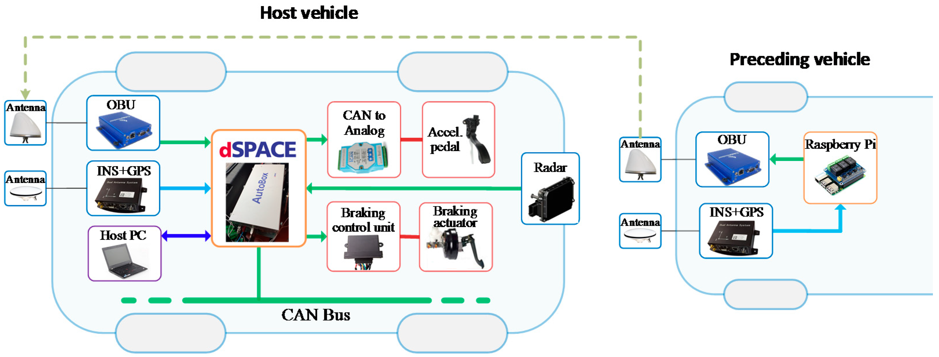
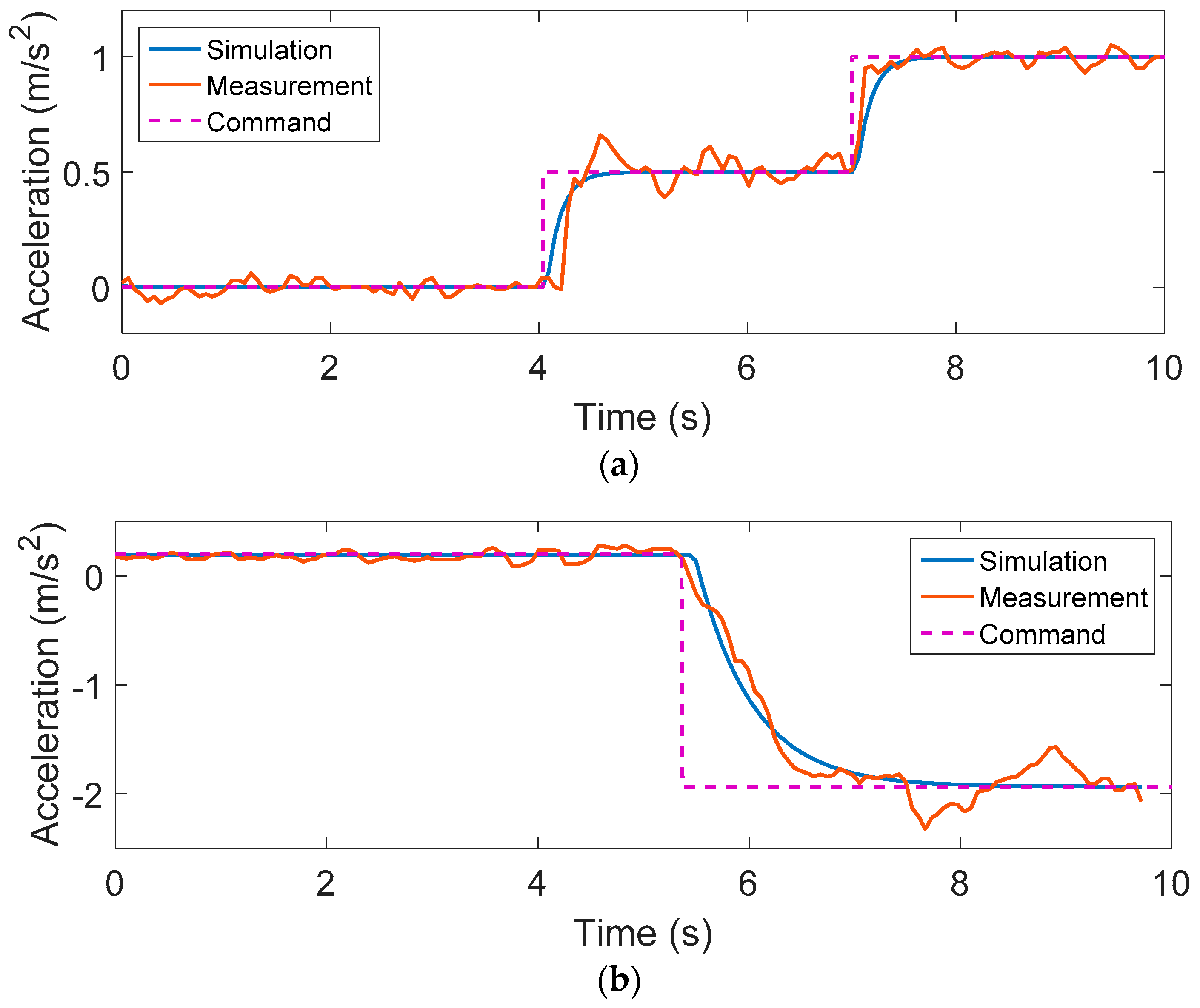
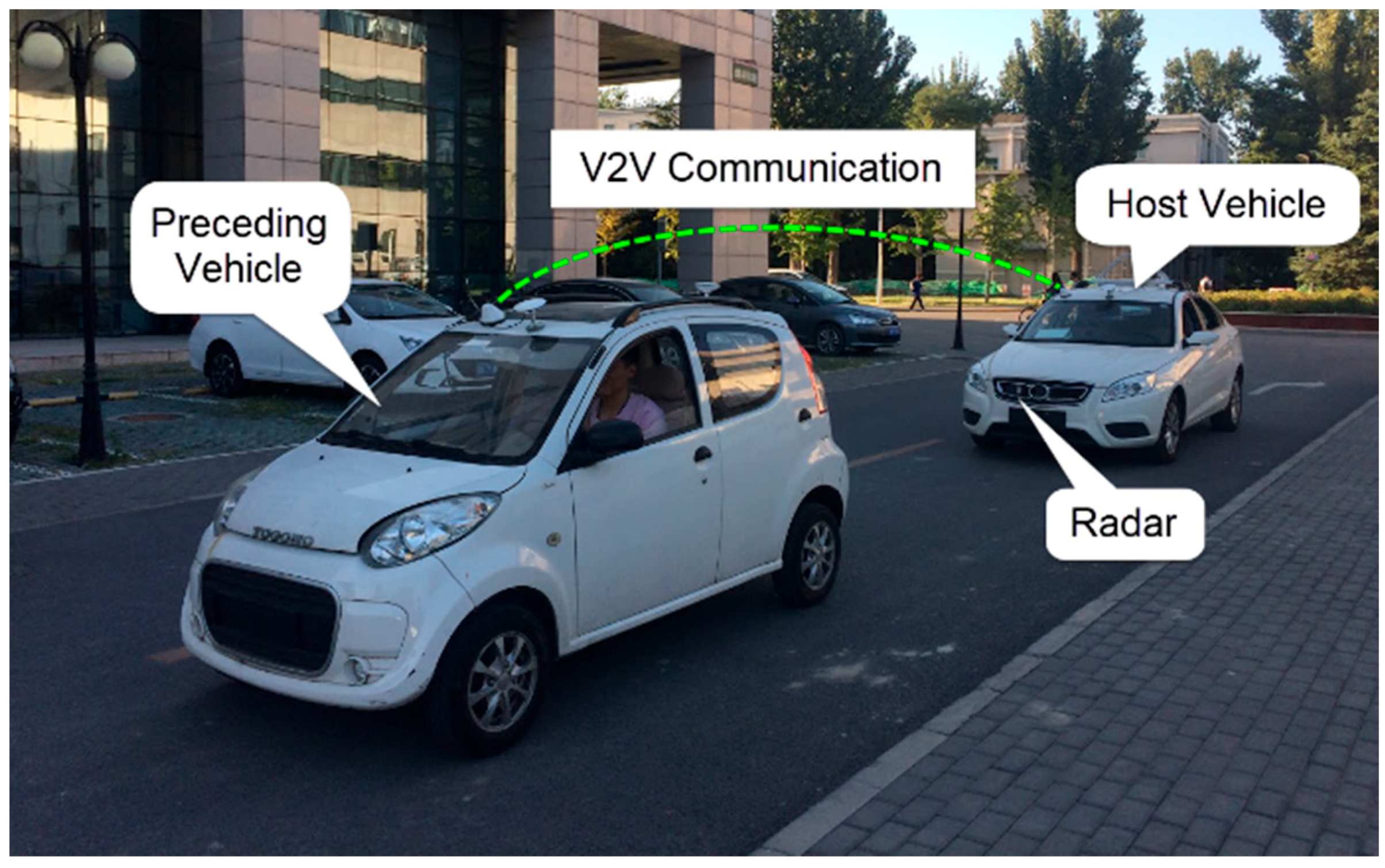
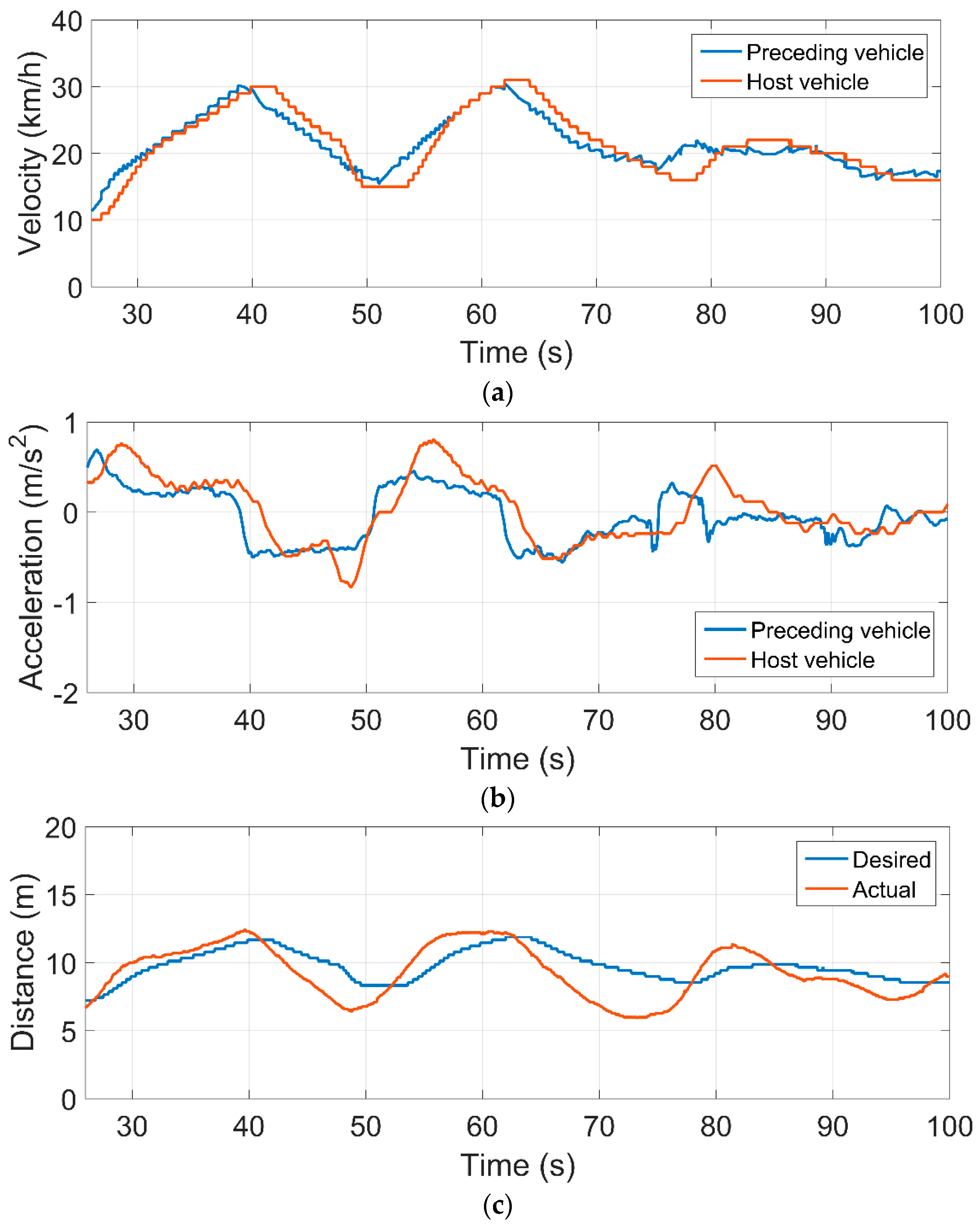
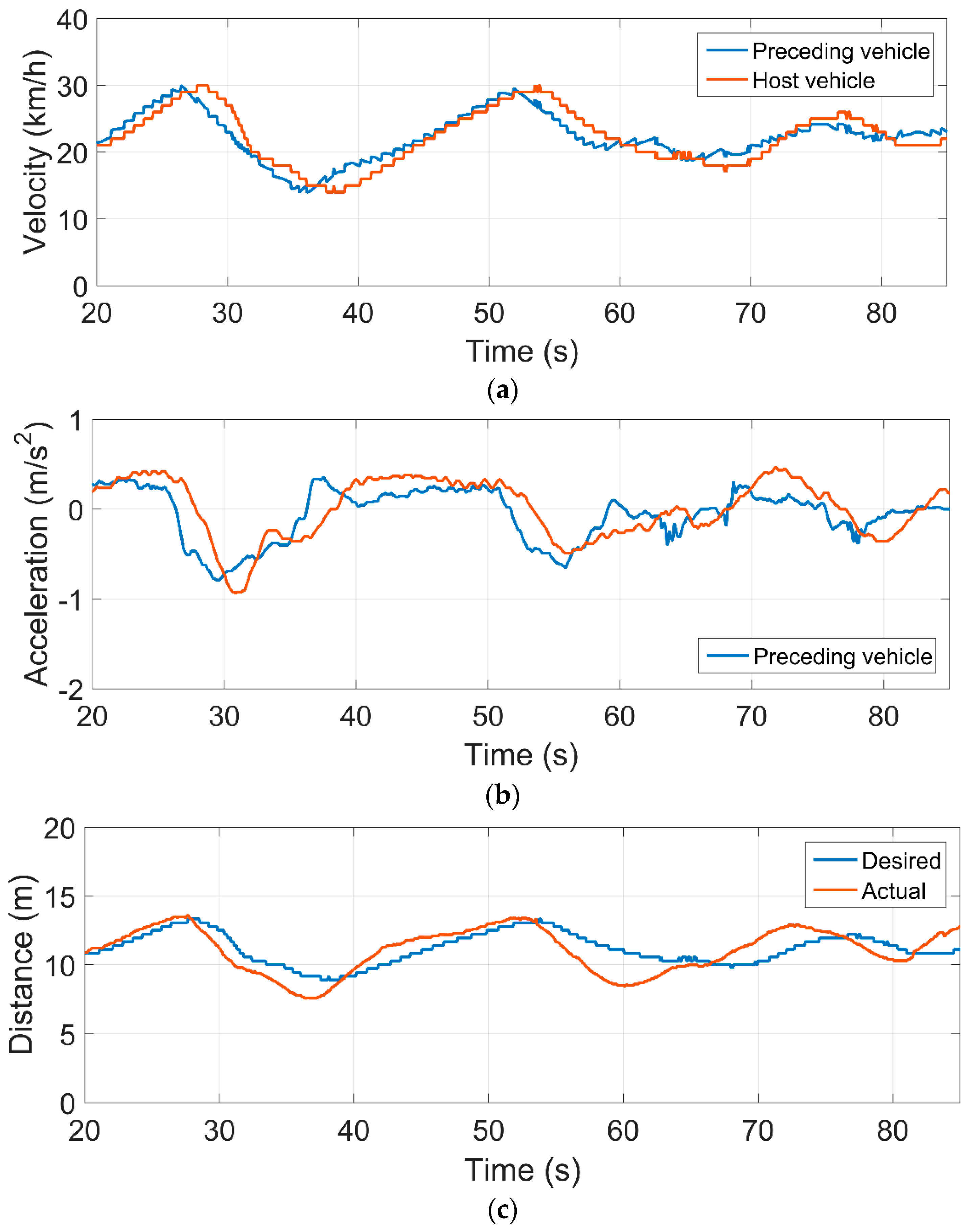
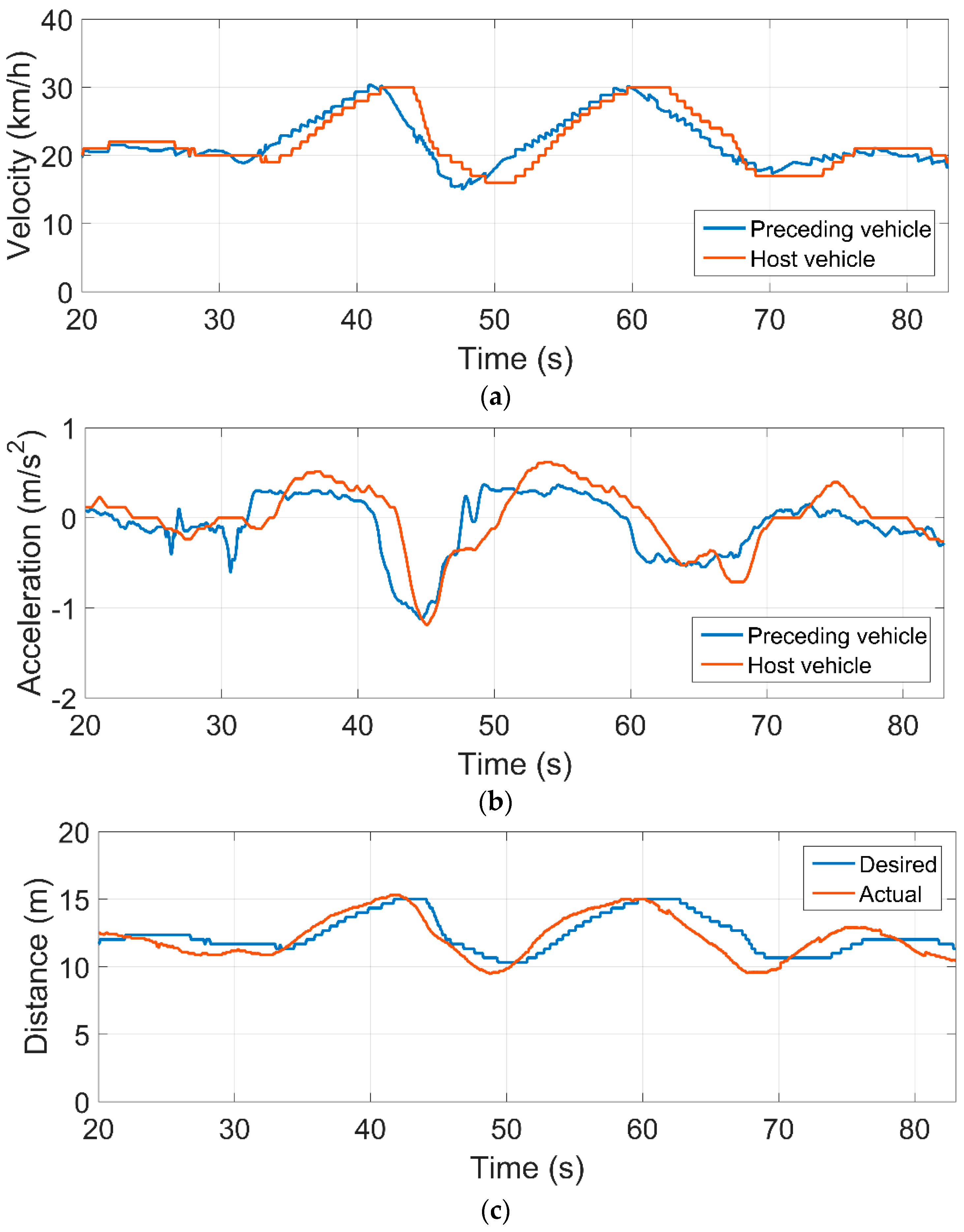
The CACC test platform is developed based on two electric vehicles (EV) and a rapid control prototyping system. The performance and learning ability of the SRL-based control policy are effectively validated by simulations and real vehicle-following experiments.
The rest of the paper is organized as follows. Section 2 describes the control framework and the test platform. Section 3 presents the SRL-based control approach for solving the CACC problem. The simulation and experimental results for a real vehicle following control are illustrated in Section 4. Section 5 concludes the paper.

2. Control Framework and Test Platform

2.1. Control Framework for CACC

The fundamental functionality of the CACC system is to regulate the acceleration of the host vehicle, such that the relative velocity between the host vehicle and its nearest preceding vehicle, and the error between the inter-vehicle distance and the desired distance, converge to zero. In this study, the control framework is designed based on a fully control-by-wire EV. Figure 1 illustrates this framework by showing that the CACC system has two separate layers. The upper level controller generates the desired acceleration a d by using input signals, including the inter-vehicle distance d r and relative velocity v r measured by radar, the acceleration of the preceding vehicle a p transmitted via V2V communication, and the velocity and acceleration of the host vehicle measured by the on-board sensor. The lower-level controller manipulates the motor output torque or the braking pressure so that the acceleration of the vehicle tracks the desired acceleration. The accelerator pedal signal α and braking pressure P b are determined by a motor torque map and a braking look-up table, respectively, which are obtained from driving tests. An incremental PID controller and the acceleration/deceleration switching logic are also included in the lower-level module, although they are not shown in the figure. A similar two-layer control framework for ACC can be found in [5].

2.2. Hardware Implementation for the Test Platform

As shown in Figure 2, the experimental platforms are built based on two electric passenger vehicles as the host vehicle and the preceding vehicle. The host vehicle, produced by the BAIC company, is front-wheel drive and equipped with a 100-kW driving motor, a single-speed gearbox, and a 41.4-kWh lithium battery pack.
A Cohda Wireless MK5 OBU (On-Board Unit), which supports the SAE J2735 DSRC standard, is used to transmit information from the preceding vehicle to the host vehicle. The data receiving and sending program, “BSM-Shell”, is run in the embedded Linux system of the OBUs. Both vehicles are equipped with the NAV-982 inertial navigation system (INS) combined with a Global Positioning System (GPS) to measure acceleration and record the position of the vehicle. On the preceding vehicle, a Raspberry Pi with extended RS232 and CAN interfaces serves as the bridge between NAV-982 and OBU for parsing the raw data from NAV-982. A Delphi 77-GHz millimeter-wave radar is installed on the front of the host vehicle to measure the distance and relative velocity of the preceding vehicle. A rapid control prototyping system is used to test the control strategy. The control algorithm is programmed in the MATLAB/Simulink environment and run in the dSPACE Autobox controller, equipped with a DS1007 processor board and a DS2202 I/O board. The control signals for acceleration and braking are sent to the lower-level control units through CAN bus. In addition, INS data parsing, radar signal processing, and the target tracking algorithm are fulfilled by the dSPACE. System states are monitored on the host PC through Ethernet. The sampling time of the system is 50 ms.

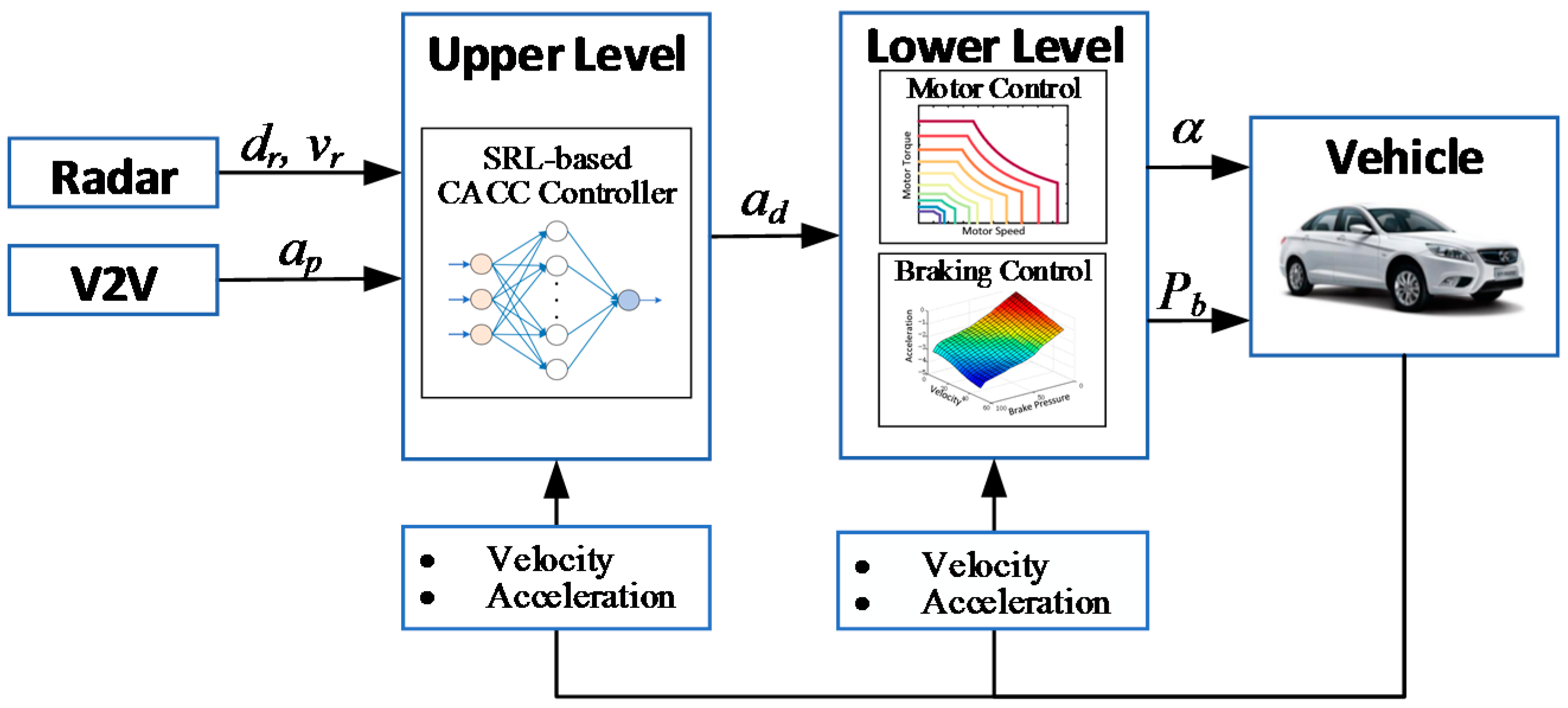
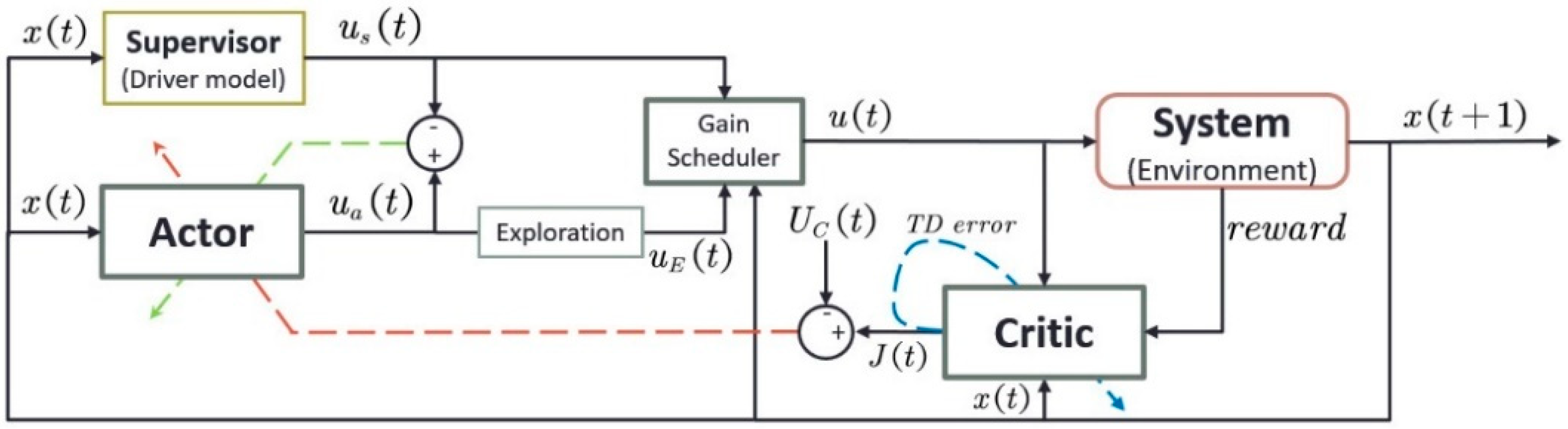
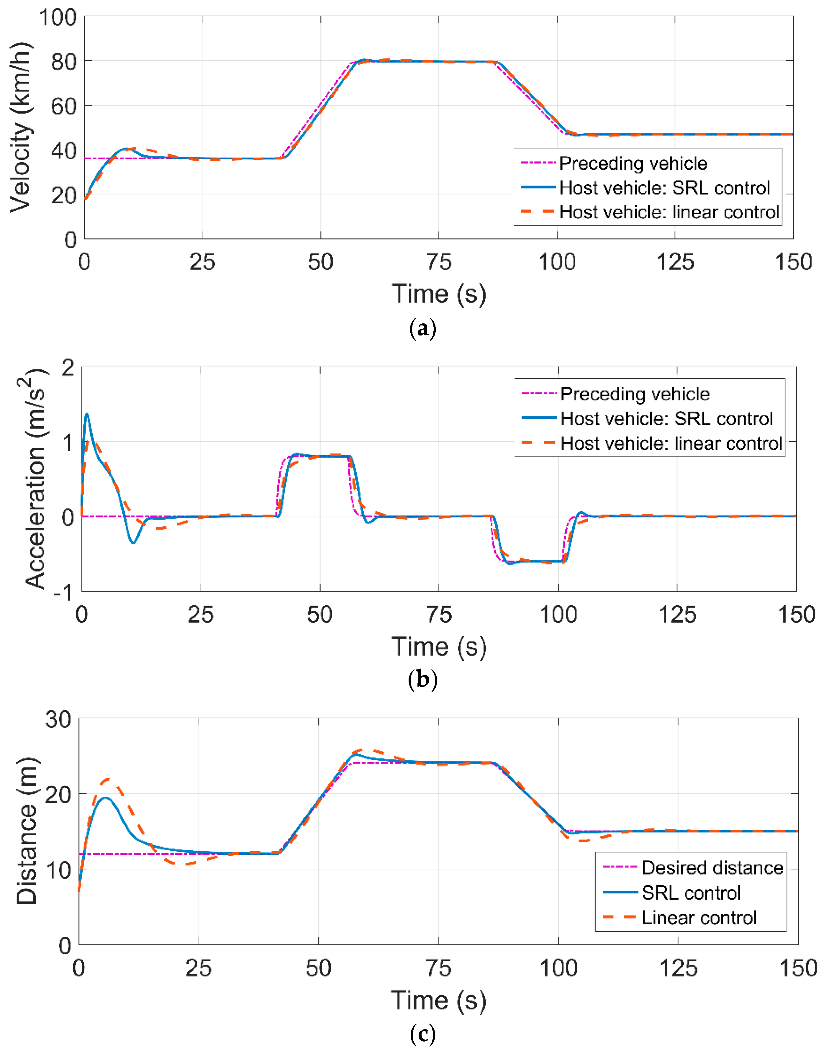
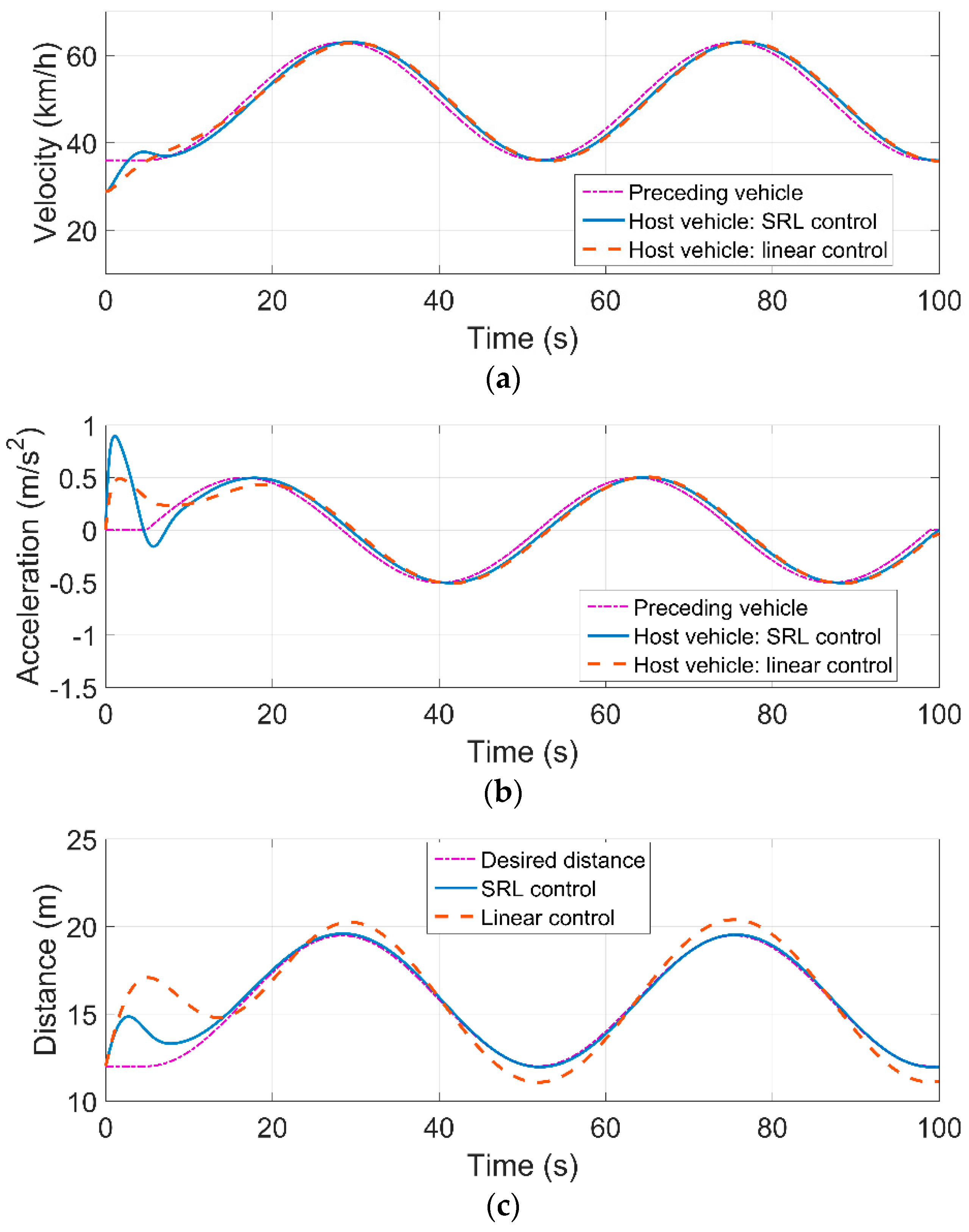
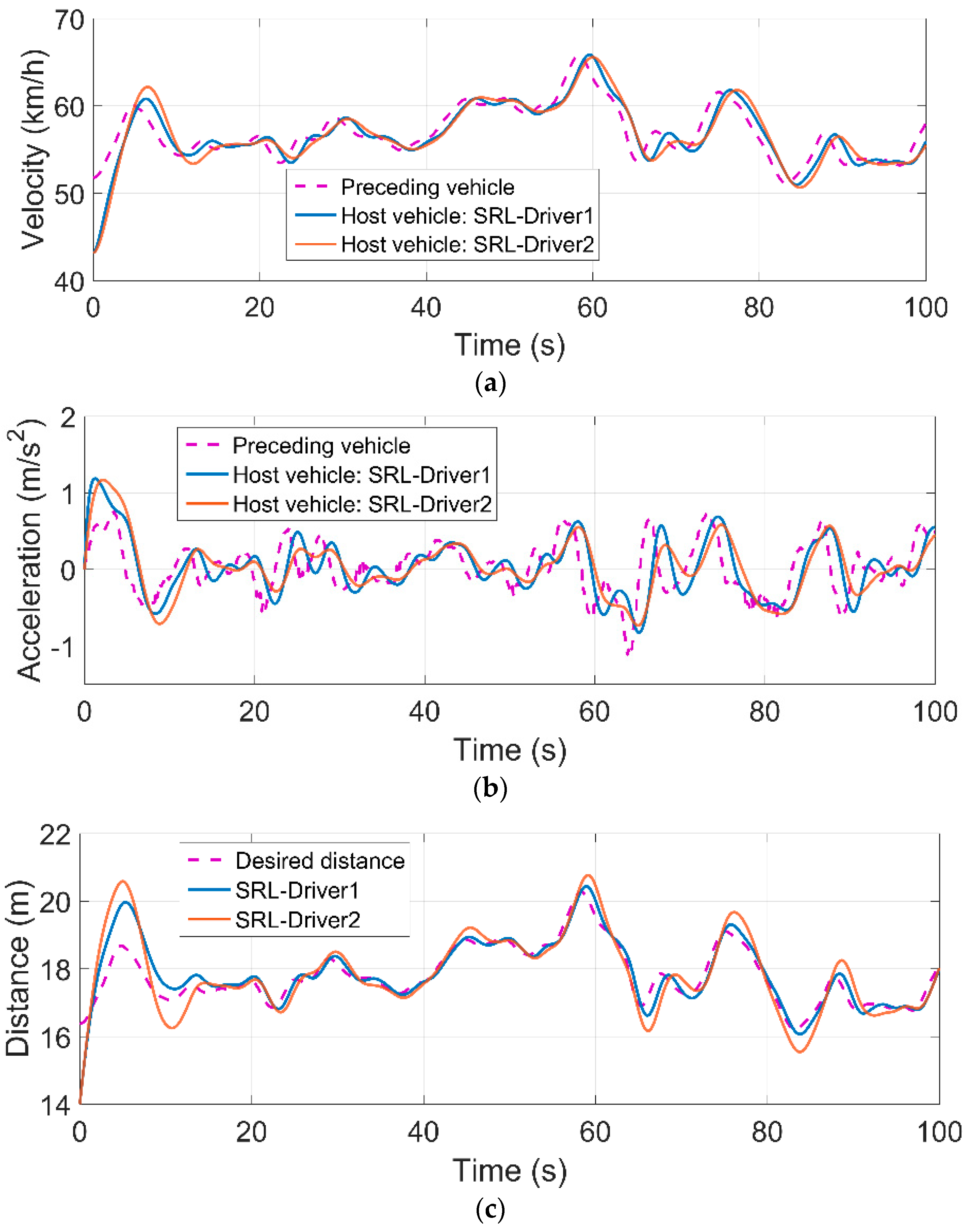
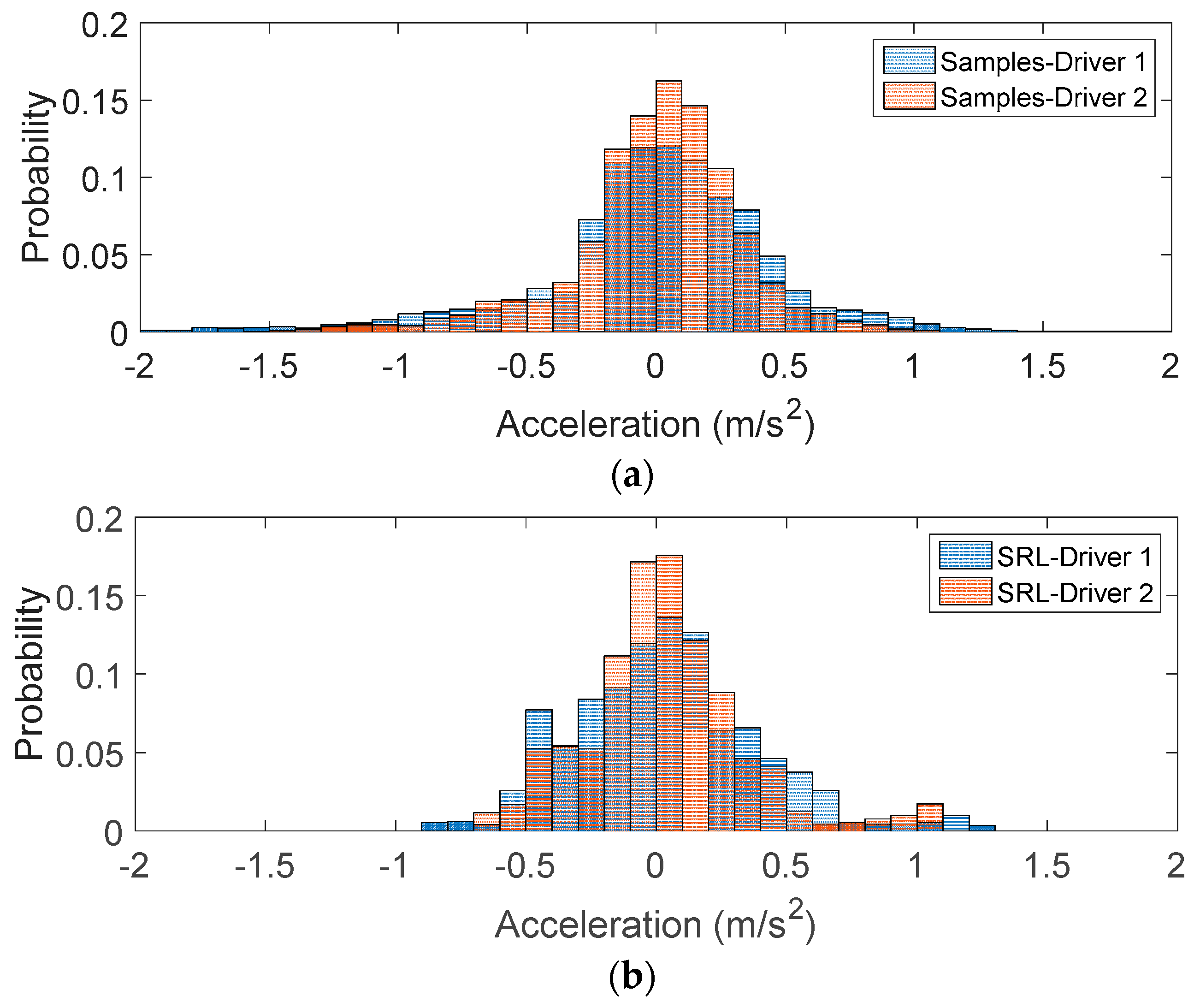
3. The SRL-Based Control Strategy for CACC

The principle of RL is learning an optimal policy, i.e., a mapping from states to actions that optimizes some performance criterion. Relying on RL alone, the learner is not told which actions to take but instead must discover which actions yield the greatest reward by trial and error [30]. Some researchers have proposed that the use of supervisory information can effectively make a learning problem easier to solve [38]. For a vehicle dynamics control problem, the richness of the human driver’s operation data can be employed to supervise the learning process of RL. In this section, an SRL-based control algorithm for CACC is proposed, as shown in Figure 3. The actor-critic architecture is used to establish the continuous relationships between states and actions and the relationships among states, actions, and the control performance [39,40]. The supervisor provides the actor with hints about which action may or may not be promising for a specific state, and the composite action blending the actions from the supervisor and the actor by the gain scheduler is sent to the system. The system responds to the input action with a transition from the current state to the next state and gives a reward to the action. More details about each module are described as follows.

3.1. System Dynamics

The primary control objective is to make the host vehicle follow the preceding vehicle at a desired distance d d ( t ) . The constant time headway spacing policy, which is the most commonly used, is adopted here [22,23,24]. The desired inter-vehicle distance is proportional to velocity:
d d ( t ) = d 0 + h v h ( t )
in which d 0 is the desired safe distance at standstill, h is the time headway, and v h ( t ) is the velocity of the host vehicle.
The longitudinal dynamics model for the host vehicle must consider the powertrain, braking system, aerodynamic drag, longitudinal tire forces, and rolling resistances, etc. The following assumptions are made to obtain a suitable control-oriented model: (1) The tire longitudinal slip is negligible, and the lower level dynamics are lumped into a first order inertial system; (2) The vehicle body is rigid; (3) The influence of pitch and yaw motions is neglected. Then, the nonlinear longitudinal dynamics can be described as
{ s ˙ h ( t ) = v h ( t ) v ˙ h ( t ) = 1 m ( η T ( t ) r C D A 21.15 v h 2 ( t ) m g f ) τ T ˙ ( t ) + T ( t ) = T d e s ( t )
in which s h ( t ) is the position of the host vehicle; m is the vehicle mass; η is the efficiency of the driveline; T ( t ) and T d e s ( t ) are the actual and desired driving/braking torque, respectively; r is the wheel radius; C D is the aerodynamic coefficient; A is the frontal area; g is the acceleration of gravity; f is the rolling resistance coefficient; and τ is the inertial delay of vehicle longitudinal dynamics.
With the exact feedback linearization technique [41], the nonlinear model (2) is converted to
T d e s ( t ) = r η ( C D A 21.15 v ( t ) ( 2 τ v ˙ h ( t ) + v h ( t ) ) + m g f + m u ( t ) )
in which u ( t ) is the control input after linearization, i.e., the desired acceleration, and we have
u ( t ) = τ a ˙ h ( t ) + a h ( t )
in which a h ( t ) = v ˙ h ( t ) denotes the acceleration of the host vehicle. The third-order state space model for the vehicle’s longitudinal dynamics is derived as
[ s ˙ h ( t ) v ˙ h ( t ) a ˙ h ( t ) ] = [ 0 1 0 0 0 1 0 0 1 / τ ] [ s h ( t ) v h ( t ) a h ( t ) ] + [ 0 0 1 / τ ] u ( t )
Using the Euler discretization approach, the state equation of continuous system (5) is discretized with a fixed sampling time Δ t as follows:
{ s h ( t + 1 ) = s h ( t ) + v h ( t ) Δ t v h ( t + 1 ) = v h ( t ) + a h ( t ) Δ t a h ( t + 1 ) = a h ( t ) Δ t τ a h ( t ) + Δ t τ u ( t )
Considering the vehicle following system of CACC, we define the system state variables as x ( t ) = [ e d ( t ) , v r ( t ) , a r ( t ) ] . e d ( t ) , v r ( t ) , and a r ( t ) are the inter-vehicle distance error, relative velocity, and relative acceleration, respectively, denoted as
{ e d ( t ) = s p ( t ) s h ( t ) d d ( t ) v r ( t ) = v p ( t ) v h ( t ) a r ( t ) = a p ( t ) a h ( t )
in which s p ( t ) , v p ( t ) , and a p ( t ) are the position, velocity, and acceleration of the preceding vehicle, respectively.
After taking the action u ( t ) in state x ( t ) , the system will go to the next state x ( t + 1 ) according to the following transition equations:
{ e d ( t + 1 ) = e d ( t ) + v r ( t ) Δ t h a h ( t ) Δ t v r ( t + 1 ) = v r ( t ) + ( a p ( t ) a h ( t ) ) Δ t a r ( t + 1 ) = a p ( t + 1 ) a h ( t ) + Δ t τ a h ( t ) Δ t τ u ( t )

3.2. The SRL Control Algorithm

There are three neural networks in the proposed SRL control algorithm: the actor, the critic, and the supervisor. The actor network is responsible for generating the control command according to the states. The critic network is used to approximate the discounted total reward-to-go and evaluate the performance of the control signal. The supervisor is used to model a human driver’s behavior and provide the predicted control signal of the driver to guide the training process of the actor and critic.

3.2.1. The Actor Network

The input of the actor network is the system state x ( t ) = [ e d ( t ) , v r ( t ) , a r ( t ) ] , and the output is the optimal action. A simple three-layered feed-forward neural network is adopted for both the actor and critic according to [39]. The output of the actor network is depicted as
u a ( t ) = f ( i = 1 N h a ω a i ( 2 ) ( t ) f i ( j = 1 n ω a i , j ( 1 ) ( t ) x j ( a ) ( t ) ) )
in which f ( ) is the hyperbolic tangent activation function; f ( z ) = ( 1 e z ) / ( 1 + e z ) , x j ( a ) denote the inputs of the actor network; ω a i , j ( 1 ) represent the weights connecting the input layer to the hidden layer; ω a i ( 2 ) represent the weights connecting the hidden layer to the output layer; N h a is the number of neurons in the hidden layer of the actor network; and n is the number of state variables.

3.2.2. The Critic Network

The inputs of the critic network are the system state x ( t ) and the composite action u ( t ) . The output of the critic, the J function, approximates the future accumulative reward-to-go value R ( t ) at time t . Specifically, R ( t ) is defined as
R ( t ) = k = 0 T α k r ( t + k + 1 )
in which α is the discount factor for the infinite-horizon problem ( 0 < α < 1 ). The discount factor determines the present value of future rewards: a reward received k time steps in the future is worth α k 1 times what it would be worth if it were received immediately [30]. T is the final time step. r ( t ) is the reward provided from the environment given by
r ( t ) = ( k 1 e d 2 ( t ) + k 2 v r 2 ( t ) + k 3 ( a h ( t ) a h ( t 1 ) ) 2 )
in which k 1 , k 2 , and k 3 are positive weighting factors. For the sake of control accuracy and driving comfort, r ( t ) is formulated as the negative weighted sum of the quadratic forms of the distance error, the relative velocity, and the fluctuation of the host vehicle’s acceleration. Thus, a higher accumulative reward-to-go value R ( t ) indicates the better performance of the action.
In the critic network, the hyperbolic tangent and linear-type activation function are used in the hidden layer and the output layer, respectively. The output J ( t ) has the following form:
u c ( t ) = i = 1 N h c ω c i ( 2 ) ( t ) f i ( j = 1 n + 1 ω c i , j ( 1 ) ( t ) x j ( c ) ( t ) )
in which x j ( c ) denote the inputs of the critic network, ω c i , j ( 1 ) represent the weights connecting the input layer to the hidden layer, ω c i ( 2 ) represent the weights connecting the hidden layer to the output layer, and N h c is the number of neurons in the hidden layer of the actor network.

3.2.3. The Supervisor

Driver behavior can be modeled with parametric models, such as the SUMO model and the Intelligent Driver Model, and non-parametric models, such as the Gaussian Mixture Regression model and artificial neural network model [42]. In [43,44], a neural network-based approach for modelling driver behavior is investigated. In this part, the driver behavior is modeled by a feed-forward neural network with the same structure as the actor network. The driver’s operation data in a real vehicle-following scenario can be collected to form a dataset D = { e d ( t ) , v r ( t ) , a r ( t ) , a d e s ( t ) } . Note that here we use the desired acceleration a d e s ( t ) as the driver’s command instead of the accelerator pedal signal α and braking pressure P b . The supervisor network can be trained with dataset D to predict the driver’s command a d e s ( t ) according to a given state [ e d ( t ) , v r ( t ) , a r ( t ) ] . The weights are updated by prediction error back-propagation, and the Levenberg-Marquardt method is employed to train the network until the weights converge.

3.2.4. The Gain Scheduler

As mentioned above, the actor network, the supervisor network, and the gain scheduler generate a composite action to the host vehicle. The gain scheduler computes a weighted sum of the actions from the supervisor and the actor as follows:
u ( t ) = k s u E ( t ) + ( 1 k s ) u s ( t )
in which u s ( t ) is the output of the supervisor, i.e., the prediction of the driver’s desired acceleration with regard to the current state. u s ( t ) is normalized within the range [−1, 1] m/s2. u E ( t ) is the exploratory action of the actor, u E ( t ) = u a ( t ) + N ( 0 , σ ) . N ( 0 , σ ) denotes a random noise with zero mean and variance σ . The parameter k s weights the control proportion between the actor and the supervisor, 0 k s 1 . This parameter is important for the supervised learning process, because it determines the autonomy level of the actor or the guidance intensity of the supervisor. Generally, the value of k s varies with the state. It can be adjusted by the actor, the supervisor, or a third party. Considering the control requirement and comfort of the driver and passengers, the range of u ( t ) , which is within the range [−1, 1], is transformed into the range [−2, 2] m/s2 before applying to the system.

3.2.5. SRL Learning

During the learning process, the weights of the actor and critic are updated with error back-propagation at each time step. After taking the composite action u ( t ) , the system transits to the next state x ( t + 1 ) and gives a reward r ( t ) . For the critic network, the prediction error has the same expression with the temporal difference (TD) error as follows:
e c ( t ) = α J ( t ) ( J ( t 1 ) r ( t ) )
The squared error objective function is calculated as
E c ( t ) = 1 2 e c 2 ( t )
The objective function is minimized by the gradient descent approach as
ω c ( t + 1 ) = ω c ( t ) + Δ ω c ( t )
Δ ω c ( t ) = l c ( t ) ( E c ( t ) ω c ( t ) ) = l c ( t ) E c ( t ) J ( t ) J ( t ) ω c ( t )
in which l c ( t ) is the learning rate of the critic network at time t , 0 < l c ( t ) < 1 .
The adaptation of the actor network is regulated by the gain scheduler. The weights of the actor are updated according to the following rule as
ω a ( t + 1 ) = ω a ( t ) + k s Δ ω a RL ( t ) + ( 1 k s ) Δ ω a SL ( t )
in which Δ ω a RL ( t ) and Δ ω a SL ( t ) are the updates based on RL and the supervised learning, respectively. The error and objective function of RL are defined as
e a RL ( t ) = J ( t ) U c ( t )
E a RL ( t ) = 1 2 ( e a RL ( t ) ) 2
in which U c ( t ) is the desired control objective. Here, U c ( t ) is set to 0, because the reward tends to zero if optimal actions are being taken.
The supervisory error and its objective function are calculated as
e a SL ( t ) = u s ( t ) u a ( t )
E a SL ( t ) = 1 2 ( e a SL ( t ) ) 2
The RL and supervisory objective functions are minimized by the gradient descent approach, and thus the reinforcement-based update and the supervisory update are calculated as
Δ ω a RL ( t ) = l a ( t ) ( E a RL ( t ) ω a ( t ) ) = l a ( t ) E a RL ( t ) J ( t ) J ( t ) u ( t ) u ( t ) ω a ( t )
Δ ω a SL ( t ) = l a ( t ) ( E a SL ( t ) ω a ( t ) ) = l a ( t ) E a SL ( t ) u a ( t ) u a ( t ) ω a ( t )
in which l a ( t ) is the learning rate of the actor network at time t , 0 < l a ( t ) < 1 .
The complete SRL algorithm is described in detail with the pseudocode as Algorithm 1.
Algorithm 1. Supervised Reinforcement Learning algorithm.
1: Collect driving samples D = { e d ( t ) , v r ( t ) , a r ( t ) , a d e s ( t ) } from a human driver in an infinite time horizon
2: Train the supervisor network with D using the Levenberg-Marquardt method
3: Input the actor and critic learning rate l a , l c ; the discount factor α ; the exploration size σ ; and the interpolation parameter k s
4: Initialize the weights of the actor and critic ω a , ω c randomly
5: Repeat for each trial
6:    x ( t ) initial state of the trial
7:   repeat for each step of the trial
8:      u s ( t ) action given by the supervisor
9:      u a ( t ) action given by the actor
10:      u E ( t ) u a ( t ) + N ( 0 , σ )
11:      k s interpolation parameter from the gain scheduler
12:      u ( t ) k s u E ( t ) + ( 1 k s ) u s ( t )
13:     execute action u ( t ) and observe the reward r ( t ) and new state x ( t + 1 )
14:      e c ( t ) α J ( t ) ( J ( t 1 ) r ( t ) )
15:     update the weights of the critic by (16) and (17)
16:      e a RL ( t ) J ( t ) U c ( t )
17:      e a SL ( t ) u s ( t ) u a ( t )
18:     update the weights of the actor by (18), (23) and (24)
19:      x ( t ) x ( t + 1 )
20:   until x ( t ) is terminal

4. Experiment Results and Discussion

4.1. Vehicle Model Validation

As described in Section 3.1, the longitudinal dynamics of the vehicle are treated as a first-order inertial system for simplicity. The inertial delay τ is identified by the step-response approach. In the driving test on a flat road, the step acceleration and braking commands are given to the lower-level controller, and the actual acceleration response is measured. The model parameters for acceleration and braking are estimated using a least-squares method as follows: τ a c c = 0.15 , τ b r a k e = 0.52 . The validation results for the identified vehicle model, as shown in Figure 4, indicate that the simulation output of the model corresponds well with the measured actual acceleration curve. Thus, the vehicle model adequately describes the longitudinal vehicle dynamics. Notably, the shorter inertial delay for acceleration is highly contributed to by the fast response of the pure electric powertrain of the test vehicle.

4.2. Training Process

First, the human driver’s manual driving data are collected with our test platform in the vehicle-following scenario. Two of our colleagues are selected to drive the host vehicle. They both have proficient driving skills but different driving styles. The first driver (Driver 1) is aggressive and tends to use large acceleration and deceleration, whereas the second driver (Driver 2) is non-aggressive, with smoother driving. The data collection for each driver lasts approximately 10 min, with a sampling time of 50 ms. The drivers commanded the vehicle with their driving habits respectively. Then, the supervisor networks with three layers and ten hidden neurons are trained by the collected samples with the MATLAB Neural Network Toolbox. The maximum number of iteration steps, performance goal, and learning rate are set as 1000, 0.001, and 0.01, respectively. Two supervisor networks with different driving styles are obtained from Driver 1 and Driver 2 for the next step.
In the SRL stage, Algorithm 1 is performed for the CACC control. It should be mentioned that the convergence analysis of the actor-critic reinforcement learning algorithm has been given in [45]. It is shown that the estimation error and the weights in the action and critic networks remain uniformly ultimately boundedness (UUB) under the given conditions. Here, the training parameters are selected on basis of UUB conditions provided by [45]. Both the actor and critic networks have three layers and ten hidden neurons. The initial learning rate of the critic and actor networks is set as 0.3 to accelerate the convergence and decreases by 0.05 at each time step until it reaches 0.003. The discount factor is 0.9. The variance σ for action exploration is 0.05. For the gain scheduler, we expect that at the beginning of the training process, the actor network is updated dominantly by the supervisor. The weight of the reinforcement update then increases gradually, such that a near-optimal policy can finally be obtained. Thus, the initial interpolation parameter k s is set as 0.2 and increases with 0.004 at each time step until it reaches 0.8. A typical driving profile is constructed as the training cycle [34,36]. In our case, the preceding vehicle starts driving at a constant velocity of 50 km/h for 50 s. Then, two step acceleration signals, 0.42 m/s2 and 0.83 m/s2, and two step deceleration signals, −0.42 m/s2 and −0.83 m/s2, are successively given; each signal lasts 20 s. At 140 s, two periods of sine wave acceleration signals are given with a 40-s period and a 1 m/s2 amplitude; then, the preceding vehicle drives at a constant velocity until the terminal time of 200 s. The initial velocity of the host vehicle is 60 km/h, and the initial inter-vehicle distance is 20 m. The host vehicle learns to follow the preceding vehicle while keeping a specific desired following range of 1 s time headway. The training step size is set as 1 s [34].
In this study, an experiment consists of a maximum of 1000 consecutive trials of the training cycle. The experiment is considered successful if the host vehicle can follow the preceding vehicle with the desired range in a steady state at the end of a trial (trial number less than 1000). For comparison, the actor-critic RL algorithm without the supervisor is also adopted for the same training process as SRL, and 100 experiments are performed for each. The training results summarized in Table 1 show that with the proposed SRL algorithm, the training process is always successful, and fewer trials are needed than with RL.

4.3. Simulation Results

The performance of the obtained control policy for CACC based on SRL is investigated via simulation with two ideal driving cycles, including the step acceleration cycle and the sinusoidal velocity cycle, and a collected real driving cycle. In [22], a linear feedforward and feedback control algorithm for CACC is proposed and tested on a vehicle. Here, the linear controller is also adopted for comparison. With the first two ideal cycles, the SRL control policy trained by samples of Driver 1 is compared with the linear control algorithm. With the real driving cycle, the SRL control policies trained by samples of Driver 1 and Driver 2 are compared to evaluate the learning ability of SRL and validate the effect of the supervisor. The time headway is set as 1 s, and the safe distance at standstill is 2 m.
Figure 5 presents the simulation results with the cycle of step accelerating and decelerating commands, followed by the maximum, average, and variance of the inter-vehicle distance error listed in Table 2. The initial distance, the initial velocity of the preceding vehicle, and the host vehicle are 7 m, 36 km/h, and 18 km/h, respectively. Note that for a fair comparison, the desired distance curve is calculated using the velocity of the preceding vehicle in this and following figures in this section. With the SRL-based control policy, the host vehicle tracks the velocity of the preceding vehicle well while maintaining the desired inter-vehicle distance. The velocity error and distance error of the SRL control policy damp more quickly compared with the linear control. More specifically, at the beginning of the simulation and the rising/falling edge of the step command, the SRL policy tends to generate a larger acceleration to achieve a faster response and more accurate inter-vehicle distance control. The maximum, average, and variance of the distance error of the SRL control policy are less than that of the linear controller, which indicates that the SRL control policy achieves a better following accuracy.
Figure 6 shows the simulation results of the sinusoidal velocity cycle. The corresponding maximum, average, and variance of the inter-vehicle distance error are listed in Table 3. At the beginning of the simulation, the SRL policy provides a larger acceleration than the linear controller to pursue the velocity of the preceding vehicle in a short period of time. After that, the SRL policy performs as well as the linear controller in velocity tracking. As shown in Figure 6c, the proposed SRL policy exceeds the linear controller in maintaining the desired distance. The distance error of SRL policy is less than the linear controller as shown in Table 3.
Moreover, the performance of the SRL control policies trained by different drivers are compared using a real driving cycle collected on an urban road in Beijing. The driving samples of Driver 1 and Driver 2 are used to train two supervisor networks, and then these two supervisors are adopted for the SRL training process to obtain two different SRL control policies. Recall that Driver 1 has an aggressive driving style, whereas Driver 2 is non-aggressive. As shown in Figure 7, both SRL policies can control the host vehicle to follow the preceding vehicle stably and accurately, and the distance error and relative velocity are regulated in a small range. The variance of distance error of the policy trained by Driver 2 (SRL-Driver2) is larger than SRL-Driver1, as listed in Table 4. The velocity curve and the acceleration curve of SRL-Driver2 are smoother than SRL-Driver1. The fluctuation range of the acceleration for SRL-Driver 1 is also larger than that of SRL-Driver 2, especially at 20 s to 40 s and 60 s to 80 s. The acceleration distribution for the data samples and simulation results are depicted in Figure 8a,b, respectively. From the acceleration distribution of the collected driving data for the two human drivers shown in Figure 8a, it can be seen that for driver 2, whose driving style is non-aggressive, the acceleration distribution is more concentrated in the areas around zero. For driver 1, the distribution probability when the absolute value of acceleration is larger than 0.5 is greater than that of driver 2. This means driver 1 tends to give larger acceleration or braking command, whereas driver 2 tends to give smaller and smoother acceleration or braking command. The distribution shapes for the data samples and the simulations results of the two drivers are clearly similar. In detail, the SRL control policy trained by Driver 2, which inherits the acceleration characteristics from the data samples of Driver 2, is more likely than SRL-Driver 1 to give small acceleration commands. It can be concluded that the SRL-based control policy learns the driving style from the samples of the human driver while guaranteeing control performance.

4.4. Test Results

Figure 9 shows the test scenario for the evaluation of the SRL-based CACC system. The host vehicle uses a millimeter-wave radar to measure the relative velocity and inter-vehicle distance. The acceleration of the preceding vehicle is sent to the host vehicle via V2V communication. Vehicle-following tests in low-speed driving situations were conducted on a flat, straight road on our campus. To validate the adaptability of the proposed control strategy, time headways of 0.8 s, 1.0 s, and 1.2 s are tested. The safe distance at standstill is set as 5 m.
The test results with different time headways for the SRL-based CACC system are shown in Figure 10, Figure 11 and Figure 12. The corresponding maximum, average, and variance of the inter-vehicle distance error are listed in Table 5. Although the velocity of the preceding vehicle fluctuates between 15 and 30 km/h, the host vehicle can always follow the velocity of the preceding vehicle accurately. The inter-vehicle distance changes according to the desired distance. Distance error occurs when the velocity of the preceding vehicle fluctuates but remains in an acceptable range. Normally, the actual distance is larger than the desired distance when the preceding vehicle accelerates and smaller than the desired value when the preceding vehicle decelerates due to the slight hysteresis of the change of the host vehicle’s velocity. The distance error and its variance decrease when a larger time headway is used, as listed in Table 5. In addition, the acceleration of the host vehicle is manipulated by the SRL controller to fluctuate closely with respect to that of the preceding vehicle. In conclusion, the effectiveness of the SRL-based CACC system is validated by vehicle-following tests with satisfactory performance.

5. Conclusions

In this study, we propose an SRL-based framework for the longitudinal vehicle dynamics control of a CACC system. A supervisor trained by driving data from a human driver is introduced to guide the reinforcement learning process. During the learning process, the composite action of the supervisor network and the actor network is sent to the system, and the actor network is updated with the error provided by the supervisor and the critic network simultaneously. The gain scheduler adjusts the weighting between supervisor and actor to improve the learning efficiency and obtain a near-optimal control policy. The simulation results show that the performance of the proposed control strategy is superior to that of the linear controller, and the human driver’s acceleration characteristics can be successfully mimicked by the SRL-based strategy, resulting in an improving driver comfort and acceptance of the CACC system. In addition, the proposed framework is demonstrated on CACC test vehicles, and the effectiveness is validated by vehicle-following tests with satisfactory performance. Notably, the SRL algorithm can be implemented in a real-time way, such that the driver’s driving data are collected for online updating of the actor network to provide a human-like control policy. In the next step, the string stability for vehicle platooning will be considered in the SRL approach to reduce the impact of the trained control policy on traffic flow.

Author Contributions

Methodology, writing, and original draft preparation: S.W.; conceptualization: S.W., Y.Z., X.Z. and W.W.; simulation and experiments: S.W., T.Z., and X.Z.; review & editing: Y.Z. and X.Z.; supervision: Y.Z.; funding acquisition: Y.Z. and W.W.

Funding

This research was funded in part by the National Key R&D Program of China under Grant 2017YFB0103801 and in part by the National Natural Science Foundation of China under Grant 51775039.

Conflicts of Interest

The authors declare no conflict of interest.

References

  1. 2013 Motor Vehicle Crashes: Overview, USDOT. Available online: https://crashstats.nhtsa.dot.gov/Api/Public/ViewPublication/812318 (accessed on 1 May 2018).
  2. National Bureau of Statistics of the PR China. 2016 China Statistical Yearbook. Available online: http://www.stats.gov.cn/tjsj/ndsj/2016/indexch.htm (accessed on 1 May 2018).
  3. Maimaris, A.; Papageorgiou, G. A review of Intelligent Transportation Systems from a communications technology perspective. In Proceedings of the 2016 IEEE 19th International Conference on Intelligent Transportation Systems (ITSC), Rio de Janeiro, Brazil, 1–4 November 2016; pp. 54–59. [Google Scholar]
  4. Zhang, J.; Wang, F.Y.; Wang, K.; Lin, W.H.; Xu, X.; Chen, C. Data-Driven Intelligent Transportation Systems: A Survey. IEEE Trans. Intell. Transp. Syst. 2011, 12, 1624–1639. [Google Scholar] [CrossRef]
  5. Moon, S.; Moon, I.; Yi, K. Design, tuning, and evaluation of a full-range adaptive cruise control system with collision avoidance. Control Eng. Pract. 2009, 17, 442–455. [Google Scholar] [CrossRef]
  6. Karagiannis, G.; Altintas, O.; Ekici, E.; Heijenk, G.; Jarupan, B.; Lin, K.; Weil, T. Vehicular Networking: A Survey and Tutorial on Requirements, Architectures, Challenges, Standards and Solutions. IEEE Commun. Surv. Tutor. 2011, 13, 584–616. [Google Scholar] [CrossRef]
  7. Chen, S.; Hu, J.; Shi, Y.; Zhao, L. LTE-V: A TD-LTE-Based V2X Solution for Future Vehicular Network. IEEE Internet Things 2016, 3, 997–1005. [Google Scholar] [CrossRef]
  8. Li, S.E.; Zheng, Y.; Li, K.; Wu, Y.; Hedrick, J.K.; Gao, F.; Zhang, H. Dynamical Modeling and Distributed Control of Connected and Automated Vehicles: Challenges and Opportunities. IEEE Intell. Transp. Syst. 2017, 9, 46–58. [Google Scholar] [CrossRef]
  9. Dey, K.C.; Yan, L.; Wang, X.; Wang, Y.; Shen, H.; Chowdhury, M.; Yu, L.; Qiu, C.; Soundararaj, V. A Review of Communication, Driver Characteristics, and Controls Aspects of Cooperative Adaptive Cruise Control (CACC). IEEE Trans. Intell. Transp. Syst. 2016, 17, 491–509. [Google Scholar] [CrossRef]
  10. Qin, W.B.; Gomez, M.M.; Orosz, G. Stability and frequency response under stochastic communication delays with applications to connected cruise control design. IEEE Trans. Intell. Transp. Syst. 2017, 18, 388–403. [Google Scholar] [CrossRef]
  11. Firooznia, A.; Ploeg, J.; van de Wouw, N.; Zwart, H. Co-design of Controller and Communication Topology for Vehicular Platooning. IEEE Trans. Intell. Transp. Syst. 2017, 18, 2728–2739. [Google Scholar] [CrossRef]
  12. Shladover, S.E.; Nowakowski, C.; Lu, X.Y.; Ferlis, R. Cooperative Adaptive Cruise Control (CACC) Definitions and Operating Concepts. Transp. Res. Rec. J. Transp. Res. Board 2015, 2489, 145–152. [Google Scholar] [CrossRef]
  13. Liu, H.; Kan, X.; Shladover, S.E.; Lu, X.Y.; Ferlis, R.E. Impact of Cooperative Adaptive Cruise Control on Multilane Freeway Merge Capacity. J. Intell. Transp. Syst. 2018, 22, 263–275. [Google Scholar] [CrossRef]
  14. Liu, H.; Kan, X.D.; Shladover, S.E.; Lu, X.Y. Using Cooperative Adaptive Cruise Control (CACC) to Form High-Performance Vehicle Streams: Simulation Results Analysis. Available online: https://escholarship.org/uc/item/31w2f555 (accessed on 6 June 2018).
  15. Rajamani, R.; Shladover, S.E. An experimental comparative study of autonomous and co-operative vehicle-follower control systems. Transp. Res. C Emerg. Technol. 2001, 9, 15–31. [Google Scholar] [CrossRef]
  16. Robinson, T.; Chan, E.; Coelingh, E. Operating platoons on public motorways: An introduction to the SARTRE platooning programme. In Proceedings of the 17th World Congress on Intelligent Transport Systems, Busan, Korea, 25–29 October 2010; Volume 1, p. 12. [Google Scholar]
  17. Solyom, S.; Coelingh, E. Performance Limitations in Vehicle Platoon Control. IEEE Intell. Transp. Syst. 2013, 5, 112–120. [Google Scholar] [CrossRef] [Green Version]
  18. Tsugawa, S.; Kato, S. Energy ITS: Another application of vehicular communications. IEEE Commun. Mag. 2010, 48, 120–126. [Google Scholar] [CrossRef]
  19. Kianfar, R.; Augusto, B.; Ebadighajari, A.; Hakeem, U.; Nilsson, J.; Raza, A.; Papanastasiou, S. Design and Experimental Validation of a Cooperative Driving System in the Grand Cooperative Driving Challenge. IEEE Trans. Intell. Transp. Syst. 2012, 13, 994–1007. [Google Scholar] [CrossRef] [Green Version]
  20. Kokogias, S.; Svensson, L.; Pereira, G.C.; Oliveira, R.; Zhang, X.; Song, X.; Mårtensson, J. Development of Platform-Independent System for Cooperative Automated Driving Evaluated in GCDC 2016. IEEE Trans. Intell. Transp. Syst. 2018, 19, 1277–1289. [Google Scholar] [CrossRef]
  21. Naus, G.J.L.; Vugts, R.P.A.; Ploeg, J.; Molengraft, M.J.G.; Steinbuch, M. String-Stable CACC Design and Experimental Validation: A Frequency-Domain Approach. IEEE Trans. Veh. Technol. 2010, 59, 4268–4279. [Google Scholar] [CrossRef]
  22. Lidström, K.; Sjoberg, K.; Holmberg, U.; Andersson, J.; Bergh, F.; Bjade, M.; Mak, S. A Modular CACC System Integration and Design. IEEE Trans. Intell. Transp. Syst. 2012, 13, 1050–1061. [Google Scholar] [CrossRef]
  23. Milanés, V.; Shladover, S.E.; Spring, J.; Nowakowski, C.; Kawazoe, H.; Nakamura, M. Cooperative Adaptive Cruise Control in Real Traffic Situations. IEEE Trans. Intell. Transp. Syst. 2014, 15, 296–305. [Google Scholar] [CrossRef] [Green Version]
  24. Geiger, A.; Lauer, M.; Moosmann, F.; Ranft, B.; Rapp, H.; Stiller, C.; Ziegler, J. Team AnnieWAY’s Entry to the 2011 Grand Cooperative Driving Challenge. IEEE Trans. Intell. Transp. Syst. 2012, 13, 1008–1017. [Google Scholar] [CrossRef]
  25. Wang, P.; Sun, Z.; Tan, J.; Huang, Z.; Zhu, Q.; Zhao, W. Development and evaluation of Cooperative Adaptive Cruise Controllers. In Proceedings of the 2015 IEEE International Conference on Mechatronics and Automation (ICMA), Beijing, China, 2–5 August 2015; pp. 1607–1612. [Google Scholar]
  26. Zheng, Y.; Li, S.E.; Li, K.; Borrelli, F.; Hedrick, J.K. Distributed Model Predictive Control for Heterogeneous Vehicle Platoons under Unidirectional Topologies. IEEE Trans. Control Syst. Technol. 2017, 25, 899–910. [Google Scholar] [CrossRef]
  27. Hu, X.; Wang, H.; Tang, X. Cyber-Physical Control for Energy-Saving Vehicle Following with Connectivity. IEEE Trans. Ind. Electron. 2017, 64, 8578–8587. [Google Scholar] [CrossRef]
  28. Rahman, M.; Chowdhury, M.; Dey, K.; Islam, R.; Khan, T. An Evaluation Strategy for Driver Car-Following Behavior Models for CACC Controllers. Transportation Research Board. 2017. Available online: https://trid.trb.org /view/1439218 (accessed on 1 May 2018).
  29. Wang, X.; Wang, Y. Human-aware autonomous control for cooperative adaptive cruise control (CACC) systems. In Proceedings of the ASME 2015 Dynamic Systems and Control Conference, Columbus, OH, USA, 28–30 October 2015; p. V002T31A001. [Google Scholar]
  30. Sutton, R.S.; Barto, A.G. Reinforcement Learning: An Introduction; MIT Press: Cambridge, UK, 1998. [Google Scholar]
  31. Xu, X.; Liu, C.; Hu, D. Continuous-action reinforcement learning with fast policy search and adaptive basis function selection. Soft Comput. 2011, 15, 1055–1070. [Google Scholar] [CrossRef]
  32. Kober, J.; Bagnell, J.A.; Peters, J. Reinforcement learning in robotics: A survey. Int. J. Robot. Res. 2013, 32, 1238–1274. [Google Scholar] [CrossRef] [Green Version]
  33. Liu, T.; Zou, Y.; Liu, D.; Sun, F. Reinforcement Learning of Adaptive Energy Management with Transition Probability for a Hybrid Electric Tracked Vehicle. IEEE Trans. Ind. Electron. 2015, 62, 7837–7846. [Google Scholar] [CrossRef]
  34. Zhao, D.; Hu, Z.; Xia, Z.; Alippi, C.; Zhu, Y.; Wang, D. Full-range adaptive cruise control based on supervised adaptive dynamic programming. Neurocomputing 2014, 125, 57–67. [Google Scholar] [CrossRef]
  35. Zhao, D.; Wang, B.; Liu, D. A supervised Actor–Critic approach for adaptive cruise control. Soft Comput. 2013, 17, 2089–2099. [Google Scholar] [CrossRef]
  36. Desjardins, C.; Chaib-draa, B. Cooperative Adaptive Cruise Control: A Reinforcement Learning Approach. IEEE Trans. Intell. Transp. Syst. 2011, 12, 1248–1260. [Google Scholar] [CrossRef] [Green Version]
  37. Huang, Z.; Xu, X.; He, H.; Tan, J.; Sun, Z. Parameterized Batch Reinforcement Learning for Longitudinal Control of Autonomous Land Vehicles. IEEE Trans. Syst. Man. Cybern. Syst. 2017, 99, 1–12. [Google Scholar] [CrossRef]
  38. Barto, M.; Rosenstein, M.T. Supervised Actor-critic Reinforcement Learning. In Handbook of Learning and Approximate Dynamic Programming; John Wiley & Sons: Toronto, ON, Canada, 2004; Volume 2, p. 359. [Google Scholar]
  39. Si, J.; Wang, Y.T. Online learning control by association and reinforcement. IEEE Trans. Neural Netw. 2001, 12, 264–276. [Google Scholar] [CrossRef] [PubMed] [Green Version]
  40. Wang, F.Y.; Zhang, H.; Liu, D. Adaptive Dynamic Programming: An Introduction. IEEE Comput. Intell. Mag. 2009, 4, 39–47. [Google Scholar] [CrossRef]
  41. Xiao, L.; Gao, F. Practical String Stability of Platoon of Adaptive Cruise Control Vehicles. IEEE Trans. Intell. Transp. Syst. 2011, 12, 1184–1194. [Google Scholar] [CrossRef]
  42. Lefèvre, S.; Sun, C.; Bajcsy, R.; Laugier, C. Comparison of parametric and non-parametric approaches for vehicle speed prediction. In Proceedings of the 2014 American Control Conference, Portland, OR, USA, 4–6 June 2014; pp. 3494–3499. [Google Scholar]
  43. Lin, Y.; Tang, P.; Zhang, W.; Yu, Q. Artificial neural network modelling of driver handling behaviour in a driver-vehicle-environment system. Int. J. Veh. Des. 2005, 37, 24–45. [Google Scholar] [CrossRef]
  44. Chong, L.; Abbas, M.M.; Flintsch, A.M.; Higgs, B. A rule-based neural network approach to model driver naturalistic behavior in traffic. Transp. Res. C Emerg. Technol. 2013, 32, 207–223. [Google Scholar] [CrossRef]
  45. Feng, L.; Sun, J.; Si, J.; Gao, W.; Mei, S. A boundedness result for the direct heuristic dynamic programming. Neural Netw. 2012, 32, 229–235. [Google Scholar]
Figure 1. Control framework for the CACC system.
Applsci 08 01014 g001
Figure 2. Functional architecture of the test platform.
Applsci 08 01014 g002
Figure 3. Schematic representation of the SRL-based CACC algorithm.
Applsci 08 01014 g003
Figure 4. Acceleration response of the host vehicle to the commanded acceleration and simulation output of the model: (a) acceleration and (b) braking.
Applsci 08 01014 g004
Figure 5. Simulation results with the cycle of step acceleration and deceleration: (a) velocity, (b) acceleration, and (c) distance.
Applsci 08 01014 g005
Figure 6. Simulation results with the cycle of sinusoidal velocity: (a) velocity, (b) acceleration, and (c) distance.
Applsci 08 01014 g006
Figure 7. Simulation results with the real driving cycle: (a) velocity, (b) acceleration, and (c) distance.
Applsci 08 01014 g007
Figure 8. Acceleration distribution for the data samples (a) and simulation results (b).
Applsci 08 01014 g008
Figure 9. Vehicle-following test scenario.
Applsci 08 01014 g009
Figure 10. Test results with an 0.8-s time headway: (a) velocity, (b) acceleration, and (c) distance.
Applsci 08 01014 g010
Figure 11. Test results with a 1.0-s time headway: (a) velocity, (b) acceleration, and (c) distance.
Applsci 08 01014 g011
Figure 12. Test results with a 1.2-s time headway: (a) velocity, (b) acceleration, and (c) distance.
Applsci 08 01014 g012
Table 1. Training results of SRL and RL.
AlgorithmNumber of ExperimentsSuccess RateAverage Number of Trials
SRL100100%128
RL10034%724
Table 2. Maximum, average, and variance of distance error, with the cycle of step acceleration and deceleration.
Control PolicyMaximum (m)Average (m)Variance
SRL control7.500.482.05
Linear control9.860.524.57
Table 3. Maximum, average, and variance of distance error, with the cycle of sinusoidal velocity.
Control PolicyMaximum (m)Average (m)Variance
SRL control2.840.230.31
Linear control5.070.431.83
Table 4. Maximum, average, and variance of distance error, with the real driving cycle.
Control PolicyMaximum (m)Average (m)Variance
SRL-Driver11.390.080.13
SRL-Driver21.930.050.30
Table 5. Maximum, average, and variance of distance error, with the real driving cycle.
Time Headway (s)Maximum (m)Average (m)Variance
0.83.41−0.432.01
1.02.54−0.121.24
1.22.50−0.100.95

