Evaluation of the Power-Law Wind-Speed Extrapolation Method with Atmospheric Stability Classification Methods for Flows over Different Terrain Types

Abstract

The atmospheric stability and ground topography play an important role in shaping wind-speed profiles. However, the commonly used power-law wind-speed extrapolation method is usually applied, ignoring atmospheric stability effects. In the present work, a new power-law wind-speed extrapolation method based on atmospheric stability classification is proposed and evaluated for flows over different types of terrain. The method uses the wind shear exponent estimated in different stability conditions rather than its average value in all stability conditions. Four stability classification methods, namely the Richardson Gradient (RG) method, the Wind Direction Standard Deviation (WDSD) method, the Wind Speed Ratio (WSR) method and the Monin–Obukhov (MO) method are applied in the wind speed extrapolation method for three different types of terrain. Tapplicability is analyzed by comparing the errors between the measured data and the calculated results at the hub height. It is indicated that the WSR classification method is effective for all the terrains investigated while the WDSD method is more suitable in plain areas. Moreover, the RG and MO methods perform better in complex terrains than the other methods, if two-level temperature data are available.

1. Introduction

In the feasibility study and microsite selection stage of wind farms, using the wind measurement data is a key step to evaluate the wind resources at the hub height. At present, wind farms are being developed towards low wind speed and high hub height. Since the height of existing wind mast towers is often lower than the hub height which results in a lack of wind data at high hub heights, it is important to develop a reliable method to evaluate the accurate wind resource for wind farm development. The motivation of wind speed extrapolation is to characterize the wind shear and the importance of wind shear characterization for wind speed calculation was mentioned in a number of studies [1,2,3].

Wind turbines typically operate at altitudes below 200 m, while the height of the convective boundary layer is on the order of 1000 m [4]. The wind shear within 100–200 m is a function of wind speed, atmospheric stability, surface roughness, and height spacing [5,6]. At present, the power law and logarithmic law are commonly used to extrapolate the wind speed. The logarithmic law can represent the vertical wind-speed profiles fairly well under neutral conditions [7] and was extended by using the Monin–Obukhov similarity theory [8] under stable or unstable conditions to include thermal stratification effects [9]. According to Optis et al. [10], the logarithmic wind-speed profile based on the Monin–Obukhov similarity theory was found inaccurate under strong stable conditions due to the shallow surface layer. For unstable conditions, Lackner et al. [11] found that the power law is robust to give a realistic wind profile than the logarithmic law.

In the near-surface layer, the wind speed affected by surface friction and atmospheric stability, varies significantly with the height [12]. Holtslag [13] analyzed the 213-m-high Cabauw meteorological tower data and found that the measured wind profile was consistent with the Monin–Obukhov similarity theory (surface layer scaling) even for the height above 100 m. Gualtieri [14] investigated the relationship between the wind shear coefficient and atmospheric stability based on the dataset recorded from the met mast of Cabauw (Netherlands), and found that the Panofsky and Dutton [15] model appeared particularly skillful during the diurnal unstable hours and during the nighttime under moderately stable conditions. Mohan and Siddiqui [16] summarized various methods for atmospheric stability classification. In the radiation method, the intensity of radiation is determined based on the amount of observed cloud which is difficult to obtain, and in the M-O length method, the heat flux data are required. In addition to these two methods, there are four methods based on the gradient Richardson number, horizontal wind standard deviation, vertical temperature gradient and wind speed ratio to classify the atmospheric stability. The parameters used in these methods can be calculated using measured wind speed, wind direction, and temperature data. Wharton and Lundquist [17] analyzed the wind farm operating data and found that, when the atmosphere was stable and the wind speed was in the range of 5~8.5 m/s, the output power was obviously greater than that in unstable conditions with strong convection, and the average difference was close to 15%. Gryning et al. [18] applied the similarity theory to establish a new model for wind-speed profile by considering the effects of atmospheric stability, and the model was applied to the height of the entire atmospheric boundary layer in a flat terrain. Đurišić and Mikulović [19] proposed a model of vertical wind-speed extrapolation for improving the wind resource assessment using the WAsP (Wind Atlas Analysis and Application Program) software [20], and found that if the estimation is carried out with the fixed wind shear exponent, the overestimated wind speed in the day time (unstable atmosphere) and underestimated wind speed in the night time (stable atmosphere) are usually obtained. Gualtieri and Secci [21] tested the power law extrapolation model over a flat rough terrain in the Apulia region (Southern Italy), and investigated the effect of atmospheric stability and surface roughness on wind speed. They found that the empirical JM Weibull distribution extrapolating model was proved to be preferable. Different extrapolating models were compared and their advantages and disadvantages were investigated. However, there are few studies on the effect of atmospheric stability on wind shear and wind speed extrapolation in different terrain types. At the same time, there are few discussions about the results of wind speed extrapolation above different ground topographies.

The present work aims to evaluate the wind speed extrapolation method using the power law and the atmospheric stability classification. For different terrain types, the characteristics of wind shear exponent are discussed, and four atmospheric stability classification methods are employed and investigated. The model is validated against the measured data, and the suitability of different atmospheric stability classification methods for flows over different types of terrain is indicated.

2. Model Description

2.1. Power Law

It is usually necessary to calculate the wind shear exponent by the wind speeds at two different levels. In the neutral condition, the wind-speed profile can be calculated using the empirical formula:

$$u\left(z\right)=\frac{u^{*}}{\kappa }\ln \frac{z}{z_0}$$

(1)

where κ is the Von Karman constant equal to 0.4, u* is the friction velocity calculated as $u^{*}={\left(\tau /\rho \right)}^{1/2}$, $\tau$ is the wall friction, $\rho$ is the density, $z_0$ is the roughness length, and $z$ is the height.

The power law (PL) method is widely used for estimating the wind speed at a wind generator hub height [22], which is defined as

$$u_2=u_1{\left(z_2/z_1\right)}^{\alpha }$$

(2)

where $u_1$ is the wind speed at the height $z_1$, $u_2$ is the wind speed at the height $z_2$, and $\alpha$ is the wind shear exponent.

From Equation (2), α can be calculated by $u_1$ and $u_2$:

$$\alpha =\ln \left(u_2/u_1\right)/\ln \left(z_2/z_1\right)$$

(3)

2.2. Atmospheric Stability Classification

The atmospheric thermal stability is suppressed or enhanced by the vertical temperature difference. The two atmospheric stability classification methods commonly used are those from Pasquill [23] and IAEA (International Atomic Energy Agency) [24]. The Pasquill method (abbreviated to P·S) proposed in the Chinese standards includes six categories: highly unstable, moderately unstable, slightly unstable, neutral, moderately stable and extremely stable. They are denoted as A, B, C, D, E, and F.

Taking the turbulence and thermal factors into account, there are three methods for classifying the atmospheric stability, namely the Monin-Obukhov method, Bulk Richardson number method, and Richardson Gradient method. Among them, theBulk Richardson number method does not have a uniform atmospheric stability classification standard, so it is not used in the present work. When the measured wind data only contains the wind direction and speed data, the wind direction standard deviation method and wind speed ratio method can be used to classify the atmospheric stability.

2.2.1. Richardson Gradient (RG) Method

The Richardson number, Ri, synthesizes the effects of thermodynamic and kinetic factors caused by the turbulence, reflecting more turbulent information [25]. Therefore, the RG method can distinguish the atmospheric stability more accurately. The Ri in the surface layer can be expressed as [26]

$$Ri=\frac{gz}{T}\frac{\Delta T}{\Delta u^2}\ln \frac{z_2}{z_1}$$

(4)

where ∆T is the difference of temperatures at $z_2$ and $z_1$. $\Delta u$ is the wind speed difference. T is the average atmospheric temperature, g is the acceleration of gravity, and z is the average geometric height calculated as $z=\sqrt{z_1{z}_2}$.

Table 1. Classification of stability based on Ri in different terrain conditions.

Stability Conditions	Mountain	Plain
A	Ri < −100	Ri < −2.51
B	−100 ≤ Ri < −1	−2.51 ≤ Ri < −1.07
C	−1 ≤ Ri < −0.01	−1.07 ≤ Ri < −0.275
D	−0.01 ≤ Ri < 0.01	−0.275 ≤ Ri < 0.089
E	0.01 ≤ Ri < 10	0.089 ≤ Ri < 0.128
F	10 ≤ Ri	0.128 ≤ Ri

shows the classification standard of Ri in different terrains [27].

Atmospheric stability depends on the net heat flux to the ground, which is equal to the sum of incident radiation, radiation emitted, latent heat, and sensible heat exchange between the atmosphere and underlying surface. When the radiation incident on the ground is dominant, the air parcels at the lower part rise, leading to a vertical air motion, and making the atmosphere unstable. Therefore, the thermal effect aggravates the air movement and prevents the wind speed from changing dramatically in the vertical direction. In this case, the Richardson number is negative. When the ground cools down, the temperature increases with increasing the height, which weakens the vertical air movement. The situation is recognized as a stable state and a positive Richardson number is obtained. The neutral stability corresponds to the case where the thermal effect is not significant. This situation occurs when the cloud is dense, and the Richardson number is zero.

2.2.2. Wind Direction Standard Deviation (WDSD) Method

The wind direction pulsation is a direct indicator of atmospheric turbulence. The magnitude of the wind direction pulsation angle is directly related to the diffusion parameter, so it can be used as an indicator to classify the atmospheric stability. However, the measurement of pulsation angle is easily influenced by the local influence of sampling location and instrument performance, which makes the method unrepresentative. So this method is more suitable for flat terrain.

Table 2. Relationship between σ_θ and the atmospheric stability.

Parameter	Atmospheric Stability
	A	B	C	D	E	F
σθ/°	σθ ≥ 22.5	22.5 > σθ ≥ 17.5	17.5 > σθ≥ 12.5	12.5 > σθ ≥ 9.5	9.5 > σθ ≥ 3.8	3.8 > σθ

shows the classification criteria recommended by Sedefian [28] based on the horizontal wind direction standard deviation, σ_θ. When σ_θ is used, the classification standard should be corrected according to the actual surface roughness. The classification standard is recommended by the United States Environmental Protection Agency (1980), and the actual area is corrected with roughness as ${\left(z_0/0.15\right)}^{0.2}$ (the corrected value is obtained by multiplying the values in Table 2).

2.2.3. Wind Speed Ratio (WSR) Method

The wind speed ratio U_R is defined as the ratio of the wind speeds at two different heights:

$$U_R=\frac{u_2}{u_1}$$

(5)

According to the rule of Pasquill stability classification, Chen [29] divided it into six categories according to the ratio of the wind speeds at two different heights (

Table 3. Relationship between U_R and the atmospheric stability.

Atmospheric Stability	A	B	C
Range	UR < 1.0032	1.0032 ≤ UR <1.0052	1.0052 ≤ UR < 1.0101
Atmospheric Stability	D	E	F
Range	1.0101 ≤ UR < 1.5717	1.5717 ≤ UR < 2.1963	UR ≥ 2.1963

).

2.2.4. Monin–Obukhov (MO) Method

In the Monin–Obukhov theory, the atmospheric stability is described by the Obukhov length L, which is determined directly from sonic anemometer measurements of friction velocity and heat flux:

$$L=-\frac{{\left(u^{\ast }\right)}^3}{\kappa \frac{g}{T}\overline{w^{\prime }{T}_S^{\prime }}}$$

(6)

where $\overline{w^{\prime }{T}_S^{\prime }}$ is the covariance of temperature and vertical wind speed fluctuations and g is the gravitational acceleration. When only the temperature gradient is available, L can be obtained by [30].

$$\{\begin{array}{ll}L=\frac{z}{Ri}& \left(Ri<0\right)\\ L=\frac{z\left(1-5Ri\right)}{Ri}& \left(Ri>0\right)\end{array}$$

(7)

According to the relationship between L and Ri,

Table 4. Classification of stability based on L in different terrains.

Stability Conditions	Mountain	Plain
A	L > −0.032	L > −0.316
B	−3.162 < L ≤ −0.032	−3.162 < L ≤ −0.316
C	−316.228 < L ≤ −31.623	−63.246 < L ≤ −3.162
D	L ≤ −316.228, L > 158.114	L ≤ −63.246, L > 158.114
E	−154.952 < L ≤ 158.114	−154.952 < L ≤ 158.114
F	L ≤ −154.952	L ≤ −154.952

shows the classification of stability based on L for flows above different terrains [27].

2.3. Wind Speed Extrapolation Method Based on Atmospheric Stability

The power law does not fully consider the effect of atmospheric stability on wind shear. According to the characteristics of atmospheric stability, the wind speed extrapolation (WSE) method based on the atmospheric stability is proposed. The measured dataset by wind towers is named as dataset Q, including time, wind speed, wind direction and wind direction standard deviation. The low wind speed data less than the cut-in wind speed in the dataset Q is first removed to obtain the filtered dataset W. Then the dataset W is classified into different stability conditions using the RG, MO, WSR, and WDSD methods. After that, Equation (3) is used to calculate the average wind shear exponent using the dataset W under each atmospheric stability condition. Finally, using the wind speeds at the lower heights in dataset Q, the higher level wind speed is predicted by Equation (2).

Four kinds of atmospheric stability classification methods, RG, WDSD, WSR and MO are adopted to develop four new methods, namely WSE-RG, WSE-WDSD, WSE-WSR and WSE-MO, for the wind speed extrapolation.

3. Cases and Measurements

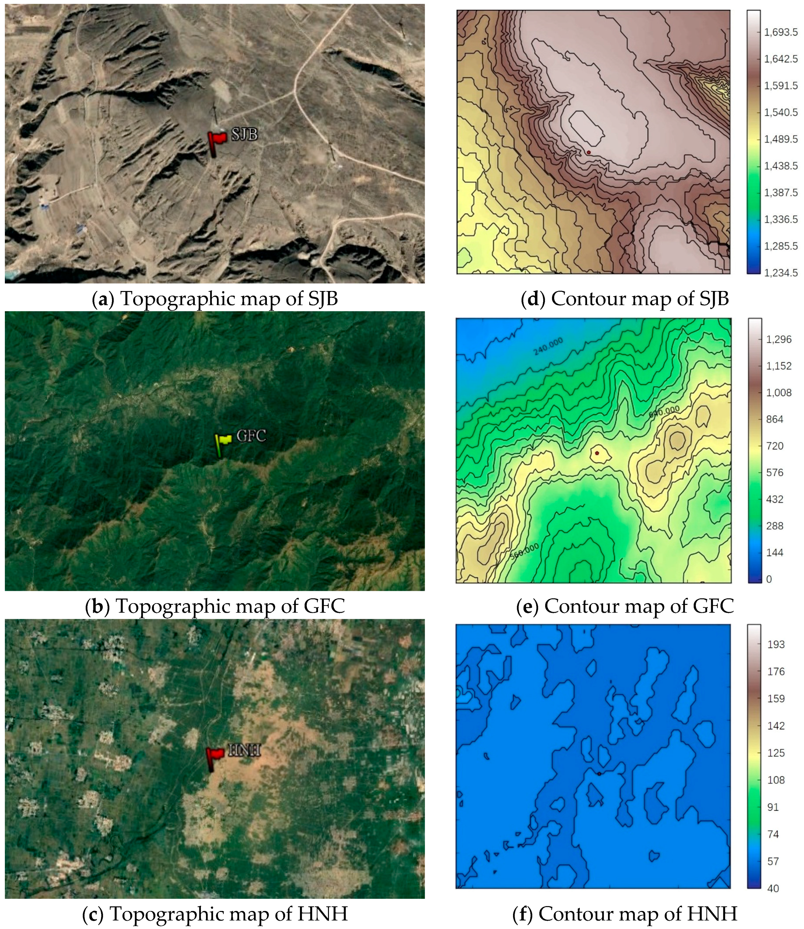
3.1. Case Definition

Three cases are chosen to test all the extrapolation methods as shown in

Table 5. Wind tower site information.

Number	Site Name	Terrain	Surface	Elevation (m)
1	SJB	Plateau	Wasteland	1678
2	GFC	Mountain	Shrubbery	713
3	HNH	Plain	Farmland	66

. The terrains include mountain, plateau and plain, and the surface types include wasteland, shrubbery and farmland.

Figure 1 shows the topographic maps of the three cases. The wind tower site SJB is located at an edge of a plateau (Figure 1a,d). The elevation of SJB in the plateau is 1678 m, and the surface type is wasteland. There is a hillside in the southwest of SJB, and flat grassland in the northeast. The GFC wind tower sits on the mountaintop, which has an altitude of 713 m (Figure 1b,e). The surface type of GFC is shrubbery. Due to the special weather conditions in the area, underlying shrub is evergreen throughout the year. The HNH wind tower is located at the elevation of 66 m, where the terrain is flat (Figure 1c,f). The land surface type is farmland and there are a large number of villages in the area.

3.2. Measurements

The wind resource in the three cases is usually measured at a site using a wind tower, equipped with wind speed and wind direction sensors. The locations of the wind towers are shown in Figure 1. The datasets of the three cases are obtained as follows:

(1)

SJB: The measured data includes wind speed, wind direction and temperature data. The cup anemometers are placed at 30, 50 and 70 m, and the wind vines are placed at 30 and 70 m. The temperature observations are also used to obtain the temperature data at 30 and 70 m.

(2)

GFC: The cup anemometers are at 30, 50 and 80 m, and the wind direction is obtained with wind vines placed at 30 and 80 m. Unfortunately, there is no temperature sensor installed on the tower.

(3)

HNH: Wind speeds are measured by the cup anemometers placed at 10, 60 and 100 m. Wind vanes are placed at 10 and 100 m. The temperature data is also unavailable in the HNH area.

The datasets at upper heights are used to verify the reliability of the wind speed extrapolation method. The measurement parameters of each case including height, time interval and data collection period are presented in

Table 6. Summary of measurement parameters.

Number	Site Name	h1 (m)	h2 (m)	h3 (m)	Time Interval (min)	Data Collection Period
1	SJB	30	50	70	10	27 August 2015~26 August 2016
2	GFC	30	50	80	10	1 August 2012~31 July 2013
3	HNH	10	60	100	10	15 September 2014~16 September 2015

.

4. Results and Discussion

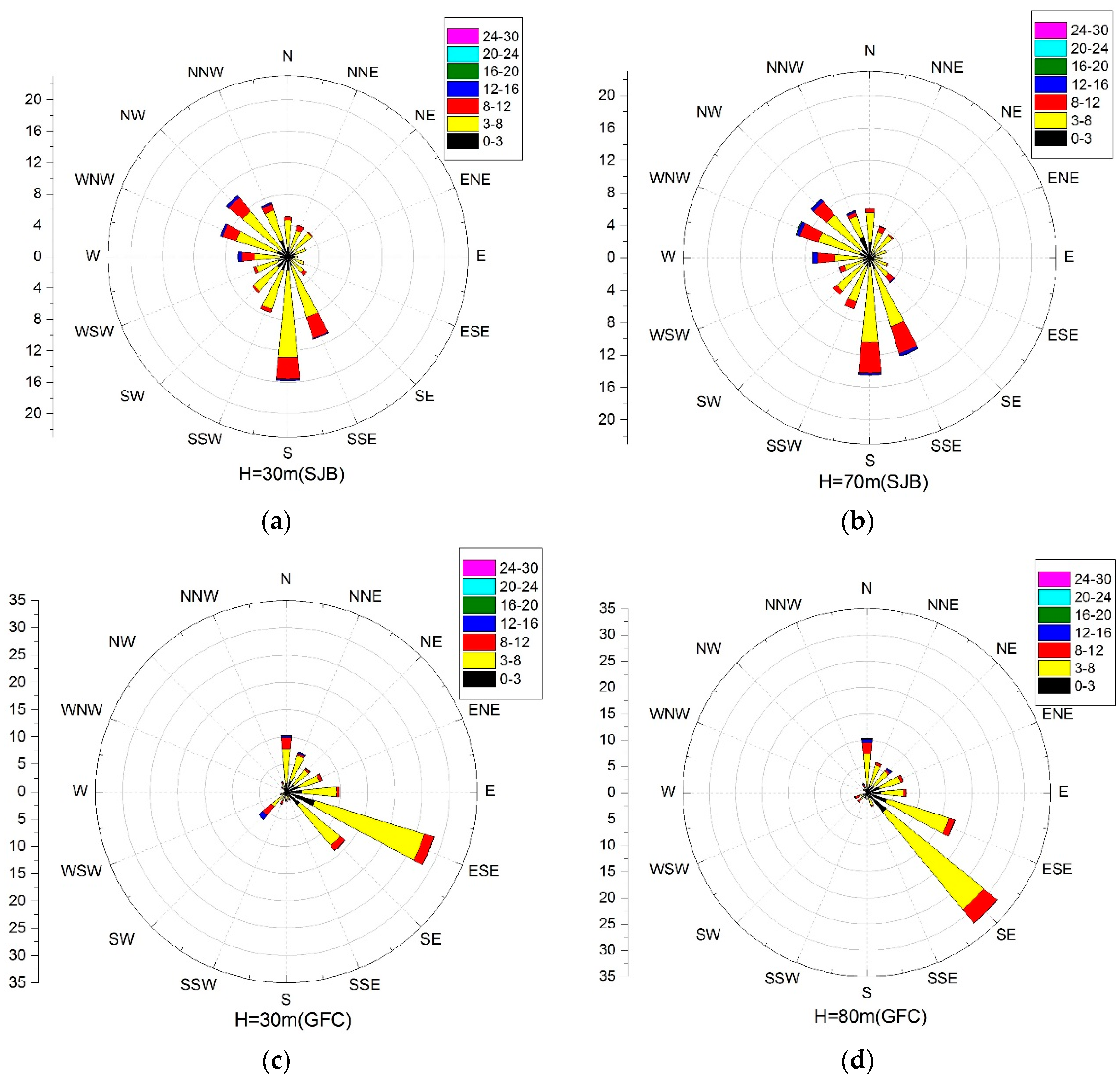
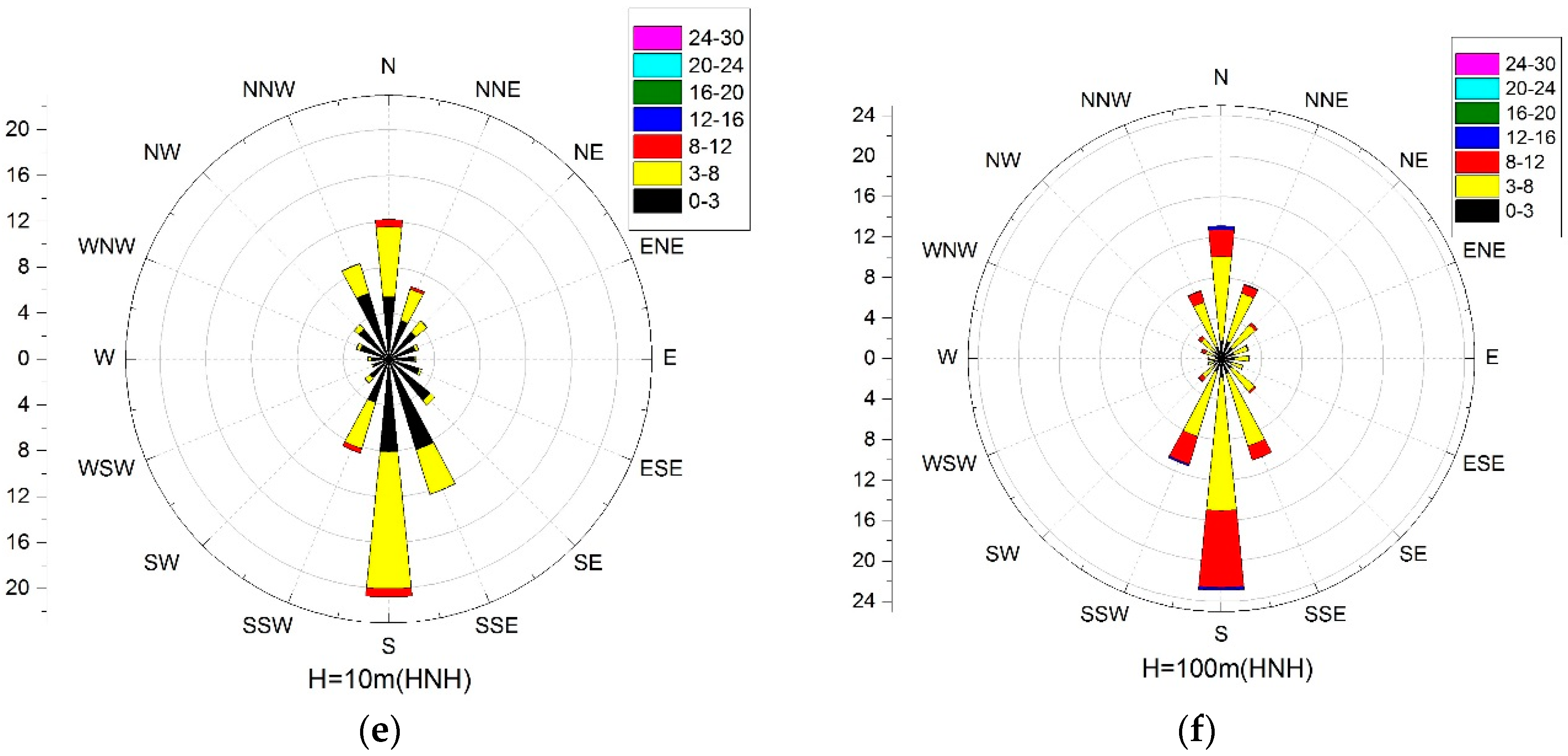
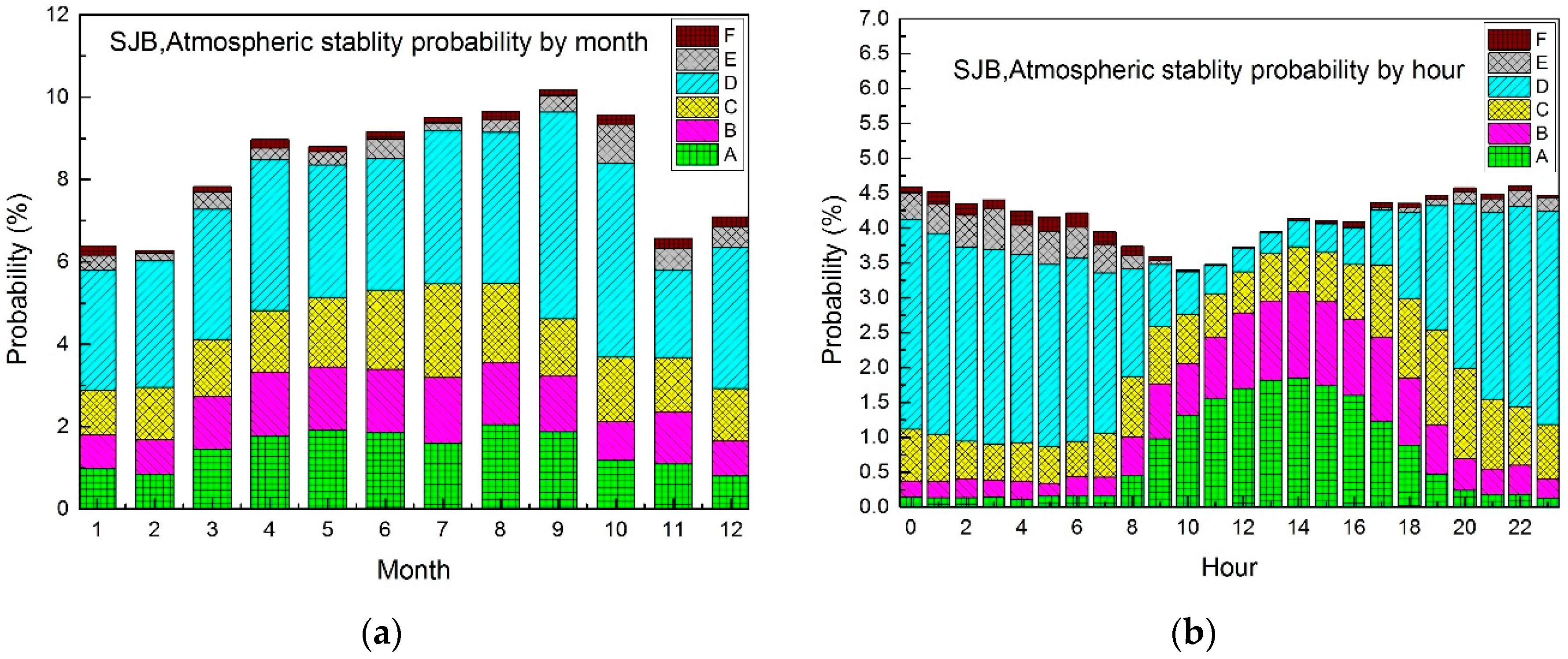
4.1. Overall Meteorological Characteristics

In

Table 7. Wind data information.

Site Name	U1 (m/s)	U2 (m/s)	U3 (m/s)	T1 (°C)	T2 (°C)	αh1–h2
SJB	5.34	5.46	5.71	8.27	8.06	0.0435
GFC	5.07	5.10	5.17	-	-	0.0115
HNH	2.73	4.61	5.44	14.30	-	0.2924

, the annual mean meteorological parameters observed for the three cases are provided where U1 and U2 are the average wind speeds at the heights of h1 and h2, U3 is the average wind speed at the hub height of h3, T1 and T2 are the mean temperatures at the heights of h1 and h2. Besides, α_h1–h2 and α_h2–h3 are the mean wind shear exponents calculated with velocities at h1 and h2, and h2 and h3 respectively.

The results indicate the difference of the wind speed distribution between the plain and mountain areas. In the HNH case, where the terrain is flat, the inconspicuous mixing of atmospheric turbulence and the weak exchange of momentum between the vertical layers result in a vertical gradient of wind speed and a large wind shear exponent. Because of the acceleration effect on the wind speed on the mountaintop, the wind shear exponents in GFC and SJB are smaller than the one in HNH.

For the SJB plateau complex terrain, at 30 m (Figure 2a) and 70 m (Figure 2b), the south direction is the most frequent wind direction with the occurrence percentages of 15.81% and 14.50%, respectively. The changes of wind speed and direction in this area are limited, because at 30 m, the wind direction is less affected by the terrain, and the height difference between the two measurement levels is only 40 m. At the same time, under the complex terrain condition, the mixing of atmospheric turbulence, the momentum exchange in the vertical direction are strong, resulting in a small wind shear exponent.

The complex topography in the GFC site strongly affects the wind behaviors at both 30 and 80 m (Figure 2c,d). At 30 m (Figure 2c), the most frequent direction is ESE (28.37%) while at 80 m (Figure 2d), the SE direction is the most frequent direction (32.17%), and ESE (17.63%) is the secondary predominant direction. At the same time, the overall wind speed interval is dominated by a low wind speed interval of 3~8 m/s. This is because the complex mountain terrain has a great impact on the wind direction. At the same time, the topographic factors also cause strong mixing in vertical, which results in smaller values of wind shear exponent, so there is no significant change in the wind speed.

For the plain area HNH, at 10 m (Figure 2e), the S direction occurs most frequently (20.75%), and at 80 m (Figure 2f), it is also the S direction (22.90%). The wind direction at 10 m and 100 m are similar, but the wind speed at 100 m is significantly higher. This is related to the flat terrain condition of this area. The atmosphere is inadequately mixed in the vertical direction in this terrain condition, which leads to a larger wind shear exponent and causes a significant change in the vertical wind speed.

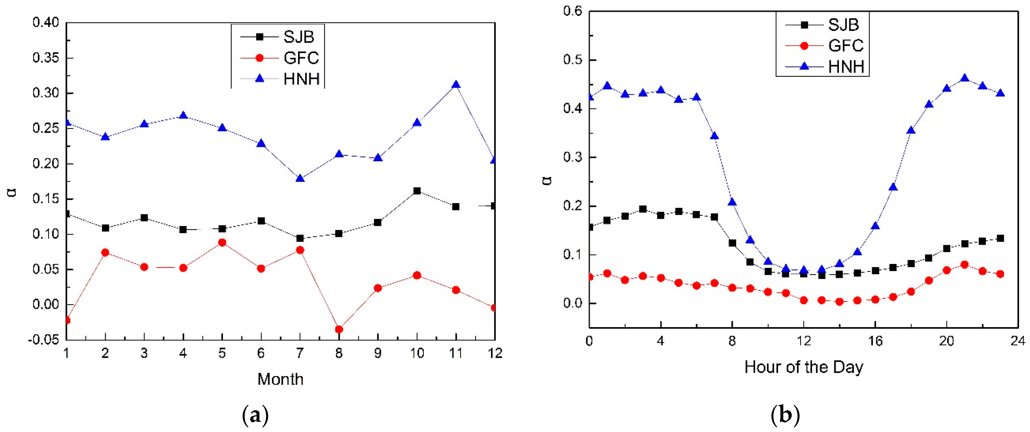
4.2. Wind Shear Characteristics of Different Terrains

Figure 3 shows the wind shear characteristics as the diurnal and monthly changes. As expected, the monthly variations of wind shear exponent at SJB and HNH are relatively high in Winter and low in Summer. The main reason is that, in Summer, the temperature is high, the mixing of near-surface air is sufficient, and the wind shear exponent is small. In Winter, the temperature is low and the air mixing is weak, usually resulting in a large wind shear exponent. However, the wind shear exponent at GFC is low in Winter and high in Summer, which deviates from the trend at SJB and HNH. This is because the area has more rains in Spring and Summer, making the air more humid and the frequency of low-level jets higher. The terrain has a dynamic lifting effect on the mountainous airflow and is prone to a strong wind shear. Furthermore, the daily change of wind shear exponent is closely related to the ambient temperature as seen in Figure 3b. The main reason for the diurnal variation of wind shear exponent is the cyclic variation of temperature. The wind shear exponent in the daytime is lower than that of the nighttime. This result is coincident with the results in the previous studies [31,32,33].

Figure 4 shows the monthly and daily variations of atmospheric stability at SJB. Comparing the atmospheric stability variation with the variation of wind shear exponent, it is found that the wind shear exponent is lower when the atmosphere is more unstable.

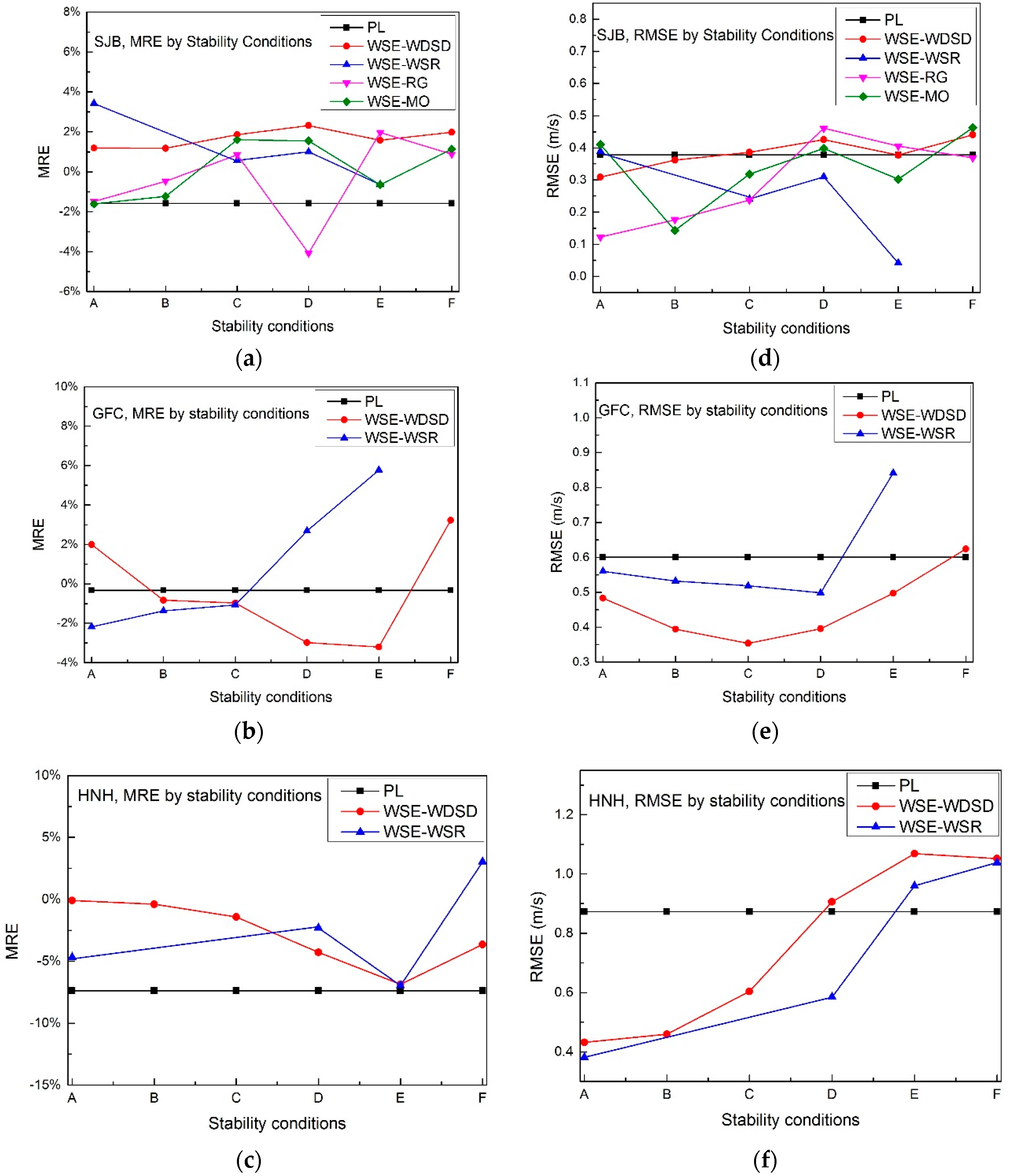
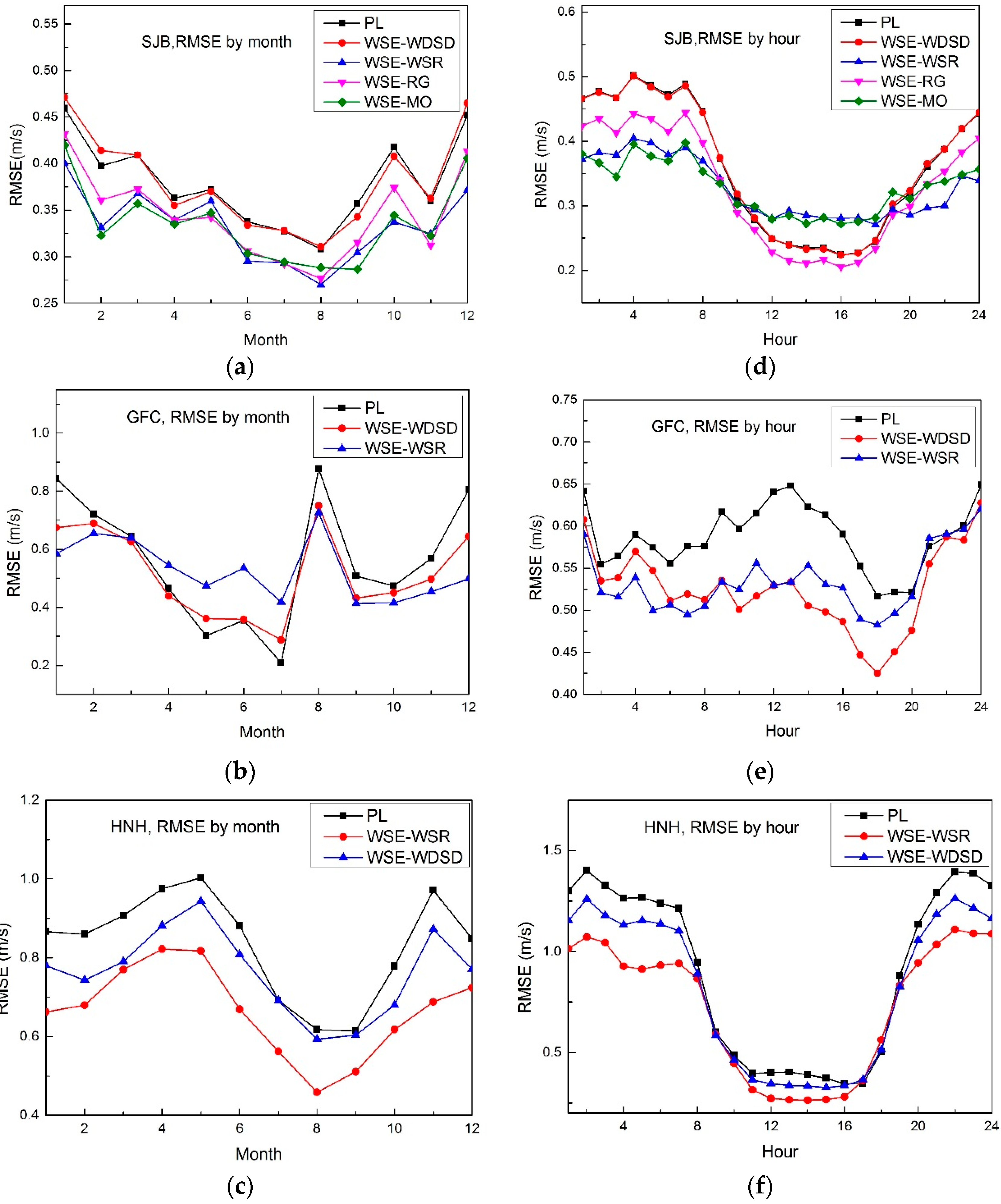
4.3. High Level Wind Speed Extrapolation and Validation

In the SJB area, starting from the 30 m and 50 m 10-min observations, the α_30–50 is calculated and then used to estimate the wind resource at a higher level. In particular, the 10-min α_30–50 is calculated using the filtered dataset W by implementing the methods of PL, WSE-RG, WSE-WDSD, WSE-WSR and WSE-MO. All the methods are adopted to calculate the wind shear exponents for the three areas and the results are listed in

Table 8. Wind shear exponents in different areas.

Area	Method	Wind Shear Exponent under Different Stability Conditions
		A	B	C	D	E	F
SJB	PL	0.0679
	WSE-RG	0.1861	0.0558	0.0676	0.3825	0.0809	0.0981
	WSE-MO	0.2875	0.0474	0.0789	0.2753	0.1156	0.0963
	WSE-WDSD	0.0648	0.0774	0.0931	0.0608	0.0779	0.0523
	WSE-WSR	0.0863	-	0.0637	0.1309	0.4704	-
GFC	PL	−0.0023
	WSE-WDSD	0.0066	0.0224	0.0307	0.0030	0.0239	-0.0175
	WSE-WSR	−0.1111	0.0081	0.0147	0.1500	0.9619	-
HNH	PL	0.1790
	WSE-WDSD	0.1466	0.1455	0.1373	0.1740	0.2587	0.3703
	WSE-WSR	−0.0079	-	-	0.1227	0.3278	0.4807
Area	Method	Wind Shear Exponent under Different Stability Conditions
		A	B	C	D	E	F
SJB	PL	0.0679
	WSE-RG	0.1861	0.0558	0.0676	0.3825	0.0809	0.0981
	WSE-MO	0.2875	0.0474	0.0789	0.2753	0.1156	0.0963
	WSE-WDSD	0.0648	0.0774	0.0931	0.0608	0.0779	0.0523
	WSE-WSR	0.0863	-	0.0637	0.1309	0.4704	-
GFC	PL	−0.0023
	WSE-WDSD	0.0066	0.0224	0.0307	0.0030	0.0239	-0.0175
	WSE-WSR	−0.1111	0.0081	0.0147	0.1500	0.9619	-
HNH	PL	0.1790
	WSE-WDSD	0.1466	0.1455	0.1373	0.1740	0.2587	0.3703
	WSE-WSR	−0.0079	-	-	0.1227	0.3278	0.4807

. At the same time, because the two-level temperature data at GFC and HNH is unavailable and the WSE-RG and WSE-MO methods cannot be used, the wind shear exponents of the two areas are calculated using the PL, WSE-WDSD, and WSE-WSR methods. It is shown that the wind shear exponent is larger under stable conditions and smaller under unstable conditions, especially in HNH. It is found that, using the WSE-WSR method, the variation of wind shear exponent with the atmospheric stability is more obvious than that using the WSE-WDSD method.

Using the results of wind shear exponent in Table 8, the wind speeds at the hub height for the three cases are also calculated. The wind speed mean relative error (MRE), root-mean-square error (RMSE) and mean wind speed at the hub height are shown in Table 8. For SJB, the MREs between the measurements and predicted wind speeds obtained by the PL, WSE-WSR, WSE-WDSD, WSE-RG and WSE-MO methods have the following sequence: MRE(PL) > MRE(WSE-WSR) > MRE(WSE-WDSD) > MRE(WSE-RG) > MRE(WSE-MO). For GFC, MRE(PL) > MRE(WSE-WSR) > MRE(WSE-WDSD). Besides, for HNH, it is MRE(PL) > MRE(WSE-WSR) > MRE(WSE-WDSD). The improvements of MRE range from 1.58 to 0.22%, 0.33 to 0.02%, 7.38 to 3.17% for the three cases using the new wind speed extrapolation methods.

It is proposed that the new WSE method based on the atmospheric stability better reflects the true changes of wind speed in two dimensions: height and time. It takes the effect of atmospheric stability on the wind profile into account and makes separate calculations for the wind resources at different conditions of atmospheric stability, which can reflect the mixing of atmosphere in the vertical direction. On this basis, the accuracy of atmospheric stability classification will directly affect the accuracy of wind speed estimation. When the two-level temperature data sets are available, it can be seen from

Table 9. Mean wind speed relative error (MRE), root-mean-square error (RMSE) of wind speed and mean speed at the hub height in the three cases.

Area	Methods	MRE	RMSE (m/s)	Calculated Mean Speed (m/s)	Measured Mean Speed (m/s)
SJB	PL	−1.58%	0.378	6.6909	6.8210
	WSE-WDSD	−1.58%	0.3781	6.6911
	WSE-MO	0.22%	0.3337	6.8229
	WSE-RG	0.63%	0.3231	6.8081
	WSE-WSR	−1.52%	0.3311	6.7242
GFC	PL	−0.33%	0.543	6.2069	6.2904
	WSE-WDSD	−0.02%	0.5276	6.2386
	WSE-WSR	−0.03%	0.536	6.2346
HNH	PL	−7.38%	0.8732	7.2567	7.5972
	WSE-WDSD	−3.17%	0.7931	7.2681
	WSE-WSR	−3.26%	0.7035	7.2815

that the WSE-RG and WSE-MO methods can better estimate the wind speed for the SJB plateau area. For the GFC mountainous area without temperature measurements, both the WSE-WDSD and WSE-WSR methods can better estimate the wind speeds and the WSE-WDSD method is more accurate than the WSE-WSR method. For the HNH plain area, where the underlying surface is farmland, both the WSE-WDSD method and WSE-WSR method can better estimate the wind speeds than the PL method.

Figure 5 shows MRE and RMSE between the measured and calculated wind speeds in different atmospheric stability conditions. For SJB, MREs and RMSEs of WSE-WDSD under different atmospheric stability conditions are close to each other and are similar to the results of PL. It can be concluded that the WDSD method cannot be applied to the complex terrain of plateau to classify the atmospheric stability. In contrast, combining the results of MREs and RMSEs, it is found that the accuracy of the WSE-RG method is improved in the cases of A, B and C, and the WSE-WSR method is suitable for the cases of C, D and E, while the WSE-MO method improves the calculation accuracy in all the conditions. For GFC, both MREs and RMSEs of the WSE-WSR method are large when the atmospheric stability condition is E. Through the comparison of RMSEs, it is seen that the WSE-WDSD method performs well in almost all the conditions. For HNH, the absolute values of MREs of the WSE-WDSD and WSE-WSR methods are smaller than those obtained by the PL method. The accuracy of both the WSE-WDSD and WSE-WSR methods has been greatly improved. It is shown that these two atmospheric stability classification methods are suitable for flat terrain. And the WSE-WSR method is more effective than the WSE-WDSD method especially in unstable conditions.

The monthly and daily variations of RMSE of the three cases using different wind speed extrapolation methods are shown in Figure 6. For SJB, the results of WSE-WDSD are very close to the traditional PL method, indicating that the WSE-WDSD method is inaccurate in the complex terrain plateau. In contrast, the results of the WSE-RG method are obviously better than those obtained by the other methods. At the same time, the results of the WSE-WSR and WSE-MO methods are similar especially for daily variations. From the daily variation, it is found that the WSE-WSR and WSE-MO methods are superior to the WSE-RG method in the night, but worse in the daytime. For the GFC and HNH, both the WSE-WDSD and WSE-WSR methods can effectively reduce RMSE, among which the WSE-WSR method is more effective. By analyzing RMSEs of the WSE-WDSD method in the HNH area where the surface is farmland, the WSE-WDSD method performs better in Winter and Spring. This is because that there are no crops in these periods, the roughness length is small, and the WDSD method is more suitable for that case.

As a result, the WSE-WSR method is confirmed to be suitable for all the above mentioned terrain types. The WSE-WDSD method is more prominent under flat terrain and mountaintop. Meanwhile, both the WSE-RG and WSE-MO methods are good choices when the measurement data has the two-level temperatures.

5. Conclusions

A new wind shear extrapolation method based on theatmospheric stability was proposed in order to calculate the wind speed at the hub height and compared with the traditional PL method. Particularly, four methods for the classification of atmospheric stability were incorporated into the WSE method. Calculations were performed for flows in three different areas, namely SJB, GFC and HNH, to verify the suitability of the proposed methods. Conclusions can be drawn as follows:

• For SJB, the plateau where the surface is wasteland, the WSE-RG, WSE-WSR and WSE-MO methods can well calculate the wind speed at the hub height. When two-level temperature data is available, the WSE-RG and WSE-MO methods are more effective, of which MRE of WSE-MO is 0.22% (MRE of PL is −1.58%) and RMSE of WSE-RG is 0.3231 m/s (RMSE of PL is 0.3780 m/s). When there are not enough temperature data, the WSE-WSR method is most effective, of which MRE is −1.52% and RMSE is 0.3311 m/s.
• For GFC, the mountain where the surface is shrubbery, the WSE-WDSD and WSE-WSR methods perform well and the WSE-WDSD method is most effective, of which MRE is −0.02% (MRE of PL is 0.33%) and RMSE is 0.5276 m/s (RMSE of PL is 0.5430 m/s).
• For HNH, the plain where the surface is farmland, the WSE-WDSD and WSE-WSR methods are also suitable. MREs of the WSE-WDSD and WSE-WSR methods are −3.17% and −3.26%, respectively (MRE of PL is −7.38%) and RMSEs of the WSE-WDSD and WSE-WSR methods are 0.7931 m/s and 0.7035 m/s, respectively (RMSE of PL is 0.6005 m/s). The WSE-WSR method is recommended when the atmosphere is unstable in most of the time.
• The new WSE model proposed in the present work has advantages over the traditional PL method. Besides, the WSE-WDSD method for extrapolating the wind speed at the hub height is more effective in plain terrain. WSE-WSR is suitable in complex terrain. Besides, the WSE-RG and WSE-MO methods have more advantages when Ri and L can be calculated.

References

1. Motta, M.; Barthelmie, R.J.; Vølund, P. The influence of non-logarithmic wind speed profiles on potential power output at Danish offshore sites. Wind Energy 2005, 8, 219–236. [Google Scholar] [CrossRef]
2. En, Z.; Altunkaynak, A.; Erdik, T. Wind Velocity Vertical Extrapolation by Extended Power Law. Adv. Meteorol. 2012, 2012, 885–901. [Google Scholar]
3. Rehman, S.; Al-Abbadi, N.M. Wind shear coefficients and their effect on energy production. Energy Convers. Manag. 2005, 46, 2578–2591. [Google Scholar] [CrossRef]
4. Huang, W.Y.; Shen, X.Y.; Wang, W.G.; Huang, W. Comparison of the Thermal and Dynamic Structural Characteristics in Boundary Layer with Different Boundary Layer Parameterizations. Chin. J. Geophys. 2015, 57, 543–562. [Google Scholar]
5. Justus, C.G. Winds and Wind System Performance; Franklin Institute Press: Philadelphia, PA, USA, 1978. [Google Scholar]
6. Irwin, J.S. A theoretical variation of the wind profile power-law exponent as a function of surface roughness and stability. Atmos. Environ. 1979, 13, 191–194. [Google Scholar] [CrossRef]
7. Troen, I.; Petersen, E.L. European Wind Atlas. Available online: http://orbit.dtu.dk/files/112135732/European_Wind_Atlas.pdf (accessed on 20 August 2018).
8. Monin, A.S.; Obukhov, A.M. Basic regularity in turbulent mixing in the surface layer of the atmosphere. Trans. Geophys. Inst. Acad. Sci. USSR 1954, 24, 163–187. [Google Scholar]
9. Jensen, N.O.; Petersen, E.L.; Troen, I. Extrapolation of Mean Wind Statistics with Special Regard to Wind Energy Applications; World Meteorological Organization: Geneva, Switzerland, 1984. [Google Scholar]
10. Optis, M.; Monahan, A.; Bosveld, F.C. Moving Beyond Monin-Obukhov Similarity Theory in Modelling Wind Speed Pro les in the Stable Lower Atmospheric Boundary Layer. Bound. Layer Meteorol. 2014, 153, 497–514. [Google Scholar] [CrossRef]
11. Lackner, M.A.; Rogers, A.L.; Manwell, J.F.; Mcgowan, J.G. A new method for improved hub height mean wind speed estimates using short-term hub height data. Renew. Energy 2010, 35, 2340–2347. [Google Scholar] [CrossRef]
12. Li, P.; Feng, C.; Han, X. Effect Analysis on the Wind Shear Exponent for Wind Speed Calculation of Wind Farms. Electr. Power Sci. Eng. 2012, 28, 7–12. [Google Scholar]
13. Holtslag, A.A.M. Estimates of diabatic wind speed profiles from near-surface weather observations. Bound. Layer Meteorol. 1984, 29, 225–250. [Google Scholar] [CrossRef]
14. Gualtieri, G. Atmospheric stability varying wind shear coefficients to improve wind resource extrapolation: A temporal analysis. Renew. Energy 2016, 87, 376–390. [Google Scholar] [CrossRef]
15. Panofsky, H.A.; Dutton, J.A. Atmospheric Turbulence: Models and Methods for Engineering Applications; Prentice-Hall: Upper Saddle River, NJ, USA, 1983. [Google Scholar]
16. Mohan, M.; Siddiqui, T.A. Analysis of various schemes for the estimation of atmospheric stability classification. Atmos. Environ. 1998, 32, 3775–3781. [Google Scholar] [CrossRef]
17. Wharton, S.; Lundquist, J.K. Atmospheric stability affects wind turbine power collection. Environ. Res. Lett. 2012, 7, 17–35. [Google Scholar] [CrossRef]
18. Gryning, S.E.; Batchvarova, E.; Brümmer, B.; Jørgensen, H.; Larsen, S. On the extension of the wind profile over homogeneous terrain beyond the surface layer. Bound. Layer Meteorol. 2007, 124, 251–268. [Google Scholar] [CrossRef]
19. Đurišić, Ž.; Mikulović, J. A model for vertical wind speed data extrapolation for improving wind resource assessment using WAsP. Renew. Energy 2012, 41, 407–411. [Google Scholar] [CrossRef]
20. Wind Resource Assessment, Siting & Energy Yield Calculations. Available online: http://www.wasp.dk/wasp (accessed on 30 July 2018).
21. Gualtieri, G.; Secci, S. Extrapolating wind speed time series vs. Weibull distribution to assess wind resource to the turbine hub height: A case study on coastal location in Southern Italy. Renew. Energy 2014, 62, 164–176. [Google Scholar] [CrossRef]
22. Hellmann, G. Über die Bewegung der Luft in den untersten Schichten der Atmosphäre; Kgl. Akademie der Wissenschaften: Copenhagen, Denmark, 1919. (In Germany) [Google Scholar]
23. Pasquill, F. Atmospheric Diffusion, 2nd ed.; Ellis Horwood: Chichester, UK, 1974. [Google Scholar]
24. Agency, I.A.E. Atmospheric Dispersion in Nuclear Power Plant Siting: A Safety Guide; International Atomic Energy Agency: Vienna, Austria, 1980. [Google Scholar]
25. Balsley, B.B.; Svensson, G.; Tjernström, M. On the Scale-dependence of the Gradient Richardson Number in the Residual Layer. Bound. Layer Meteorol. 2008, 127, 57–72. [Google Scholar] [CrossRef]
26. Ma, Y. The basic physical characteristics of the atmosphere near the ground over the Qinghai-Xizang Plateau. Acta Meteorol. Sin. 1987, 2, 188–200. [Google Scholar]
27. Deng, Y.; Fan, S.J. Research on the surface layer’s stability classifying schemes over coastal region by Monin-Obukhov length. In Proceedings of the National Conference on Atmospheric Environment, Nanning, China, 25 October 2003; pp. 136–141. [Google Scholar]
28. Sedefian, L.; Bennett, E. A comparison of turbulence classification schemes. Atmos. Environ. 1980, 14, 741–750. [Google Scholar] [CrossRef]
29. Chen, P. A comparative study on several methods of stability classification. Acta Sci. Circumstantiae 1983, 3, 77–84. [Google Scholar]
30. Businger, J.A. Flux profile relationships in the atmospheric surface layer. J. Atmos. Sci. 1971, 28, 181–189. [Google Scholar] [CrossRef]
31. Rehman, S.; Al-Abbadi, N.M. Wind shear coefficient, turbulence intensity and wind power potential assessment for Dhulom, Saudi Arabia. Renew. Energy 2008, 33, 2653–2660. [Google Scholar] [CrossRef] [Green Version]
32. Greene, S. Analysis of vertical wind shear in the Southern Great Plains and potential impacts on estimation of wind energy production. Int. J. Energy Issues 2009, 32, 191–211. [Google Scholar] [CrossRef]
33. Fox, N.I. A tall tower study of Missouri winds. Renew. Energy 2011, 36, 330–337. [Google Scholar] [CrossRef]
Figure 1. Topographic maps of three cases: (a) SJB; (b) GFC and (c) HNH; Contour maps of the three cases: (d) SJB; (e) GFC and (f) HNH.
Applsci 08 01429 g001
Figure 2. Wind rose measured at the three sites: (a) 30 m at SJB; (b) 70 m at SJB; (c) 30 m at GFC; (d) 80 m at GFC; (e) 10 m at HNH; (f) 100 m at HNH.
Applsci 08 01429 g002aApplsci 08 01429 g002b
Figure 3. Monthly and diurnal variations of h1–h2 wind shear exponents in the three cases: (a) monthly variation; (b) diurnal variation.
Applsci 08 01429 g003
Figure 4. Probability of atmospheric stability classification at SJB: (a) monthly variation; (b) daily variation.
Applsci 08 01429 g004
Figure 5. (ac) MREs and (df) RMSEs between the measured and calculated values under different atmospheric stabilities conditions in the three different areas.
Applsci 08 01429 g005
Figure 6. (ac) Monthly and (df) daily variations of RMSE using different methods in the three different cases.
Applsci 08 01429 g006