Analysis and Impact Evaluation of Missing Data Imputation in Day-ahead PV Generation Forecasting


1
School of Integrated Technology, Gwangju Institute of Science and Technology, Gwangju 61005, Korea
2
Research Institute for Solar and Sustainable Energies, Gwangju Institute of Science and Technology, Gwangju 61005, Korea
*
Author to whom correspondence should be addressed.
Appl. Sci. 2019, 9(1), 204; https://0-doi-org.brum.beds.ac.uk/10.3390/app9010204
Submission received: 6 December 2018
/
Revised: 30 December 2018
/
Accepted: 31 December 2018
/
Published: 8 January 2019
(This article belongs to the Special Issue Applications of Artificial Neural Networks for Energy Systems)
Abstract
:Over the past decade, PV power plants have increasingly contributed to power generation. However, PV power generation widely varies due to environmental factors; thus, the accurate forecasting of PV generation becomes essential. Meanwhile, weather data for environmental factors include many missing values; for example, when we estimated the missing values in the precipitation data of the Korea Meteorological Agency, they amounted to ~16% from 2015–2016, and further, 19% of the weather data were missing for 2017. Such missing values deteriorate the PV power generation prediction performance, and they need to be eliminated by filling in other values. Here, we explore the impact of missing data imputation methods that can be used to replace these missing values. We apply four missing data imputation methods to the training data and test data of the prediction model based on support vector regression. When the k-nearest neighbors method is applied to the test data, the prediction performance yields results closest to those for the original data with no missing values, and the prediction model’s performance is stable even when the missing data rate increases. Therefore, we conclude that the most appropriate missing data imputation for application to PV forecasting is the KNN method.
1. Introduction
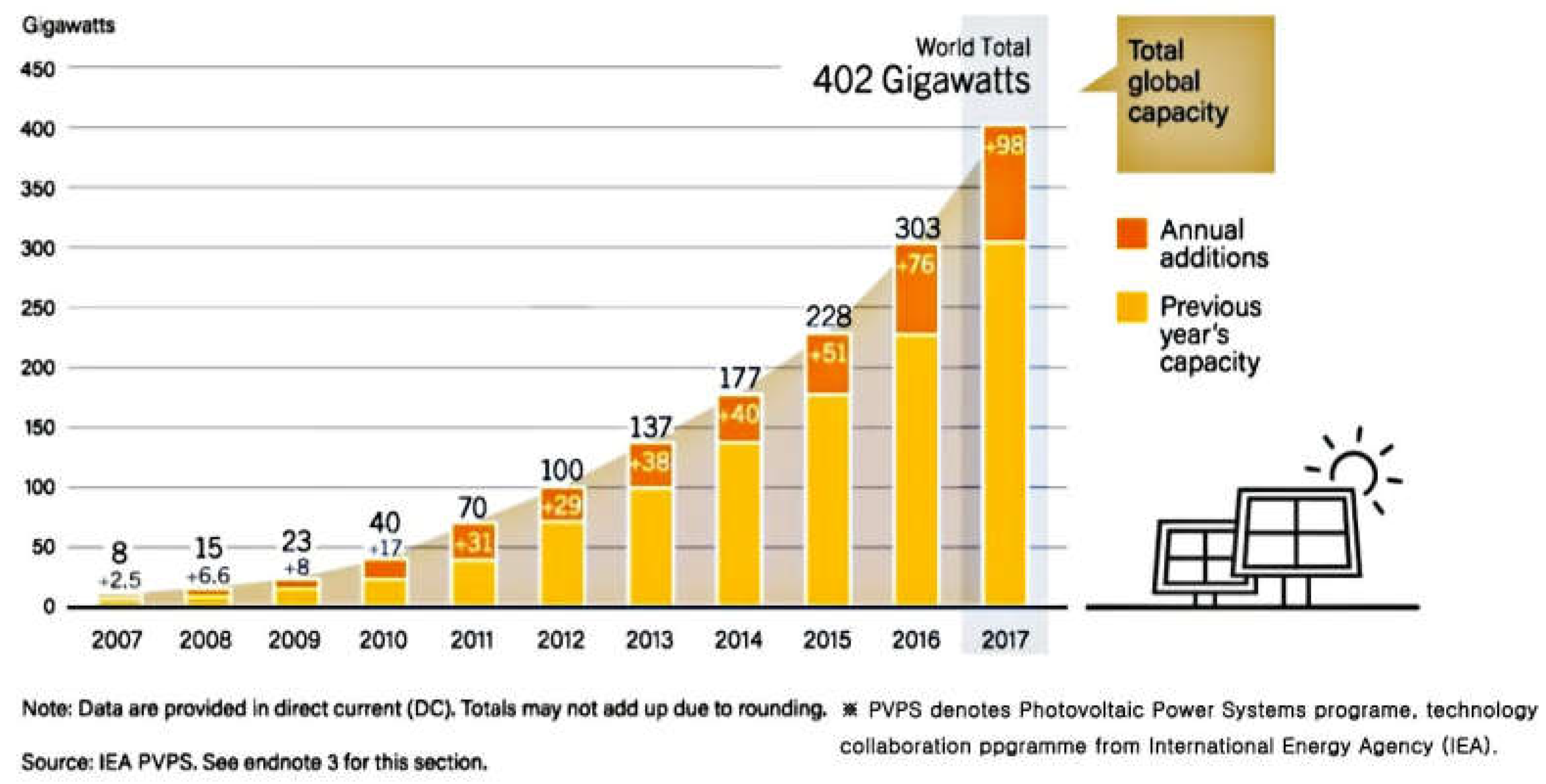
With photovoltaic (PV) systems becoming a mature and environmentally-friendly technology over the past few years, several countries have begun to invest aggressively in PV energy resources. For example, China has increased its PV budget by 30.7% of that of 2017. In addition to developed countries such as China, developing ones such as the Marshall Islands, Rwanda, and the Solomon Islands are also increasingly investing in renewable energy [1], thereby leading to increased PV generation over the past decade [2]. Figure 1 [1] depicts the increasing trend of PV power generation, which implies that PV systems are expected to spread globally.
However, PV generation depends on weather conditions such as temperature, relative humidity, precipitation, and solar radiation. In other words, the PV output fluctuates frequently because of weather factors. With more PV systems integrating with grids, such fluctuating PV generation can severely impact the stability, reliability, quality, and system operation of power systems while also reducing economic benefits. Therefore, the accurate forecasting of PV generation becomes very important for grid operations involving distributed energy resources. As mentioned in [3], several studies have focused on the prediction of solar power generation and solar radiation in this context. Among the 15,700 solar irradiation and power prediction articles appearing in a Google Scholar search, 6340 were published in 2016.
However, there are still problems in accurately forecasting solar power generation because of inaccurate predictions arising due to missing data, where “missing data” refers to completely absent data objects/series or imperfect data, i.e., partial data [4]. In this context, it has been reported [5] that when the missing data ratio in the total data is less than 1%, the impact is negligible. Further, missing rates between 1% and 5% correspond to manageable or flexible sample data. On the other hand, missing data rates >5% of the total data require suitable solutions [5]. Further, missing data rates of >15% significantly adversely affect the prediction model [6,7]. Thus far, PV power generation prediction studies have reported poor performances on rainy days relative to sunny days [8,9,10]. This implies that the existence of many missing precipitation data values significantly deteriorates the prediction accuracy. Hence, methods to address the missing data need to be urgently studied.
Several studies on missing data imputation have been conducted in multiple contexts. In [5,6,7,11,12], missing data imputation algorithms based on statistical methods and machine learning approaches such as the k-nearest neighbors (KNN) method have been proposed. Other studies [13,14,15,16] have proposed missing data imputation methods for solar irradiation. In [13], the authors proposed three missing data imputations that can replace missing data for solar radiation: inverse-distance weighting (IDW), multiple linear regression (MLR), and multivariate imputation by chain equations (MICE). Among these, MICE affords outputs closest to the original solar radiation values when the missing values are replaced. In [14], the authors estimated the temperature and relative humidity for solar irradiance prediction using the Fourier series and support vector machines (SVMs), while in [15], the authors examined several missing weather data imputation methods ranging from simple ones such as mean imputation to complicated ones such as the multilayer perceptron and Markov chain Monte Carlo approaches. In [16], the authors devised two missing imputation methods using atmospheric temperature and relative humidity: the decision matrix and the regression correlation of weather data. The first method affords a minimum correlation coefficient value of 0.95, RMSE of 87.6 W/, NRMSE of 8.29%, and an index of agreement of 0.97 for irradiation. Here, NRMSE is the value obtained by dividing the RMSE value by the difference between the maximum and the minimum values of measured irradiation data. On the other hand, the second method yields higher error than the first method. In addition to research on solar radiation, several research works have focused on meteorological factors [17,18,19,20]. In [17], the authors demonstrated the drawbacks of the IDW method and proposed three other methods: the coefficient correlation weighing method (CCWM), the artificial neural network estimation method (ANNEM), and the kriging estimation method (KEM), which outperformed conventional methods. Meanwhile, another study [18] has suggested the fixed functional set genetic algorithm method (FFSGAM), which utilizes genetic algorithms and nonlinear optimization methods to estimate the missing data. When compared with IDW, the FFSGAM yields greater prediction accuracy. Here, we note that only six rain-gauging stations in Korea are able to estimate missing data; thus, missing data imputation becomes extremely important in this context. The method proposed in [19] is similar to that in [17] in that both are based on hybrid models. The former approach utilizes an artificial neural network (ANN) and a regression tree (RT) and affords better prediction accuracy than the ANN or RT models alone. Meanwhile, in [20], the authors demonstrated 17 deterministic missing data imputations for missing precipitation data and concluded that the most suitable method is multiple linear regression weighted by the square of the missing data ratio.
Several studies have demonstrated improved prediction performance via application of these methods to classification or prediction models [21,22]. In [21], the authors demonstrated a neural network model of breast cancer diagnosis with the use of three statistical methods and three missing data machine learning methods. In [22], the authors demonstrated that the conventional road traffic congestion prediction performance can be improved via application of a missing data imputation method based on machine learning techniques.
However, very few studies have applied missing weather data imputation to PV generation forecasts. Although in [23], the authors developed a PV forecasting model using missing data imputation methods, they only considered missing PV power data imputation, and not missing weather data imputation. Missing data imputation forms a significant data preprocessing issue in predicting solar power generation because precipitation data are generally inaccurate. For example, as per the Korea Meteorological Administration, the approximate missing data rate was 16% in 2015 and 2016 and 19% in 2017. In particular, it is difficult to estimate how rainfall must be considered because a large amount of precipitation data is missing. However, very few researches have focused on how solar power generation forecasts change when the missing-point replacement method is applied.
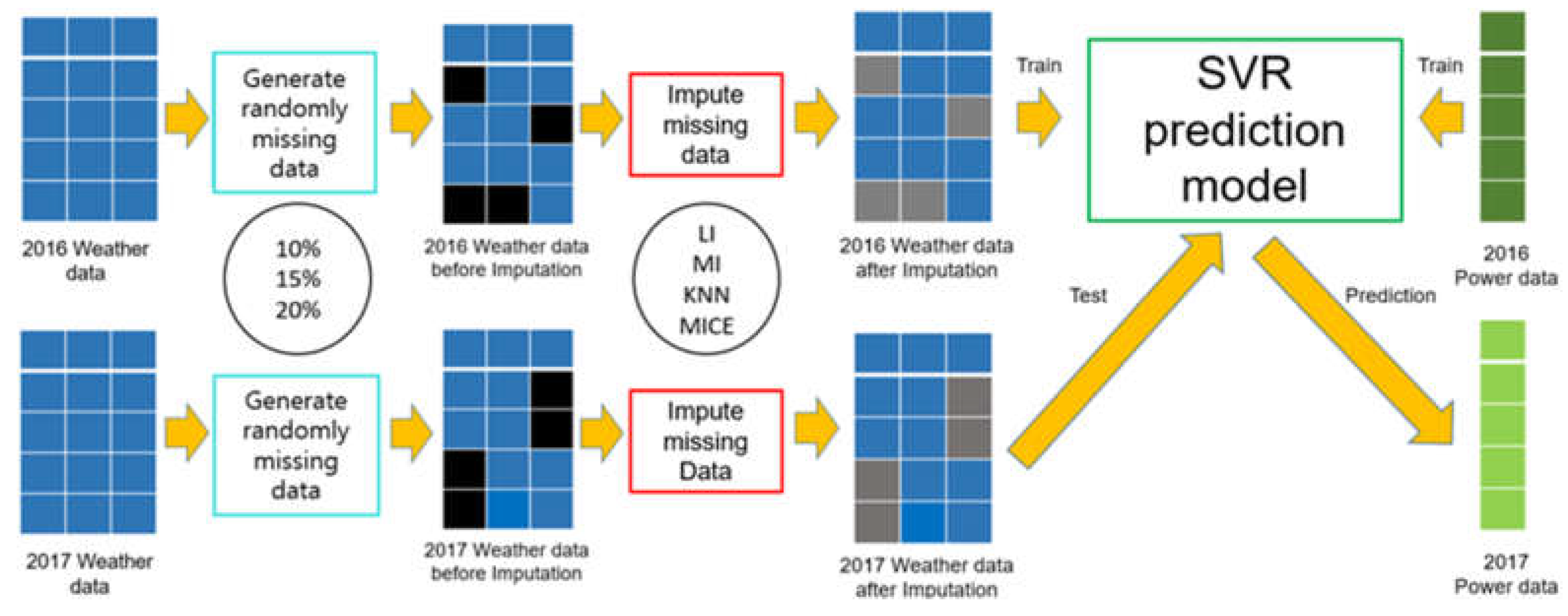
Against this backdrop, here, we generate randomly missing data in the weather data of the period of 2016–2017 with three missing data ratios, corresponding to the missing completely at random (MCAR) process [24]. Next, we replace the missing data with suitable values by using four different approaches, linear interpolation (LI), mode imputation (MI), k-nearest neighbors (KNN), and multivariate imputation by chain equations (MICE). Thirdly, for four cases that utilize the missing data imputation methods and one that does not do so, we construct forecasting models using the SVR method with the solar power generation data for 2016. Finally, we predict solar PV generation for 2017 with the forecasting model and missing value-corrected weather data of 2017. Further, we calculate and compare the forecast errors for a specific period in 2017, and we examine the accuracy resulting from the application of the missing data imputation methods.
The rest of the paper is organized as follows: Section 2 describes the meteorological and historical PV power generation data used in predicting solar power generation along with the four missing data imputation methods. Section 3 describes the error evaluation performance of the missing data imputation methods applied to the model. In Section 4, we calculate the error of the missing data imputation for each method and present the results. Finally, Section 5 concludes the paper.
2. Forecasting Model and Missing Data Imputation Methodology
2.1. Data and Prediction Model
The solar power generation data are based on the PV dataset provided by the Korea Southern Power Co., Ltd. (KOSPO). The dataset can be downloaded in the CSV, JSON, etc., file formats from the Korea Open Data Portal [25]. The time step of the data is 1 h, and it covers the period from 1 January 2015–19 September 2017. In this study, the data from 1 January–31 December 2016 are used as the PV power prediction model training data, and data from 1 January–19 September 2017 are used as test data. The solar power plant of interest is located at 55, Hwasunhaean-ro 106 beon-gil, Andeok-myeon, Seogwipo-si, Jeju-do, Republic of Korea (around latitude 33.24° and longitude 126.34°). The peak output PV power of the plant is 196 kW.
The meteorological hourly data can be downloaded by use of the open weather data portal provided by the Korea Meteorological Administration [26]. In the study, we used the local live forecast data of Jeju Island. The weather conditions included temperature, relative humidity, wind speed, wind direction, precipitation, and sky condition. Here, the sky condition expresses the amount of cloud cover as a numerical value in the range from 1–4, where 1 indicates the least cloud cover and 4 the highest cloud cover. As in the case of 1-h time-step power generation data, 1-h time-step weather data of 2016 were used to train the prediction model, and 1-h time-step weather data for 2017 were used for the tests. Time and month values were used in the model to capture the time and seasonal characteristics not reflected by weather variables. Here, we mention that the weather data factor most closely related to solar power generation is solar irradiance. However, meteorological data portals do not provide the predicted solar irradiance data. Therefore, we used the solar irradiance data from the Python Library (PVLIB) [27]. The library was utilized as follows: First, we defined the time zone of solar radiation data to be obtained. We next calculated the zenith and azimuth angles with time by inputting time data into the get_solarposition function of PVLIB with the time zone. Next, we used the get_clearsky function of PVLIB to calculate various solar radiation data such as global horizontal irradiation (GHI), direct normal irradiation (DNI), and diffuse horizontal irradiation (DHI). A detailed description cab be found in [28]. We note here that it is possible to compute the solar irradiation amount per hour at the PV panel location on sunny days by combining the three solar irradiation datasets, the Sun’s zenith angle, azimuth, latitude, longitude, time zone, tilt of the solar panel, and azimuth information of the surface. The azimuth information corresponds to the plane of array irradiance components on a tilted surface. This value does not reflect weather conditions. Even though it is not considered in solar radiation, we estimate that this factor can be predictable even on days with cloudy weather, because the prediction model is learned by using the predicted amount of precipitation and cloud amount data.
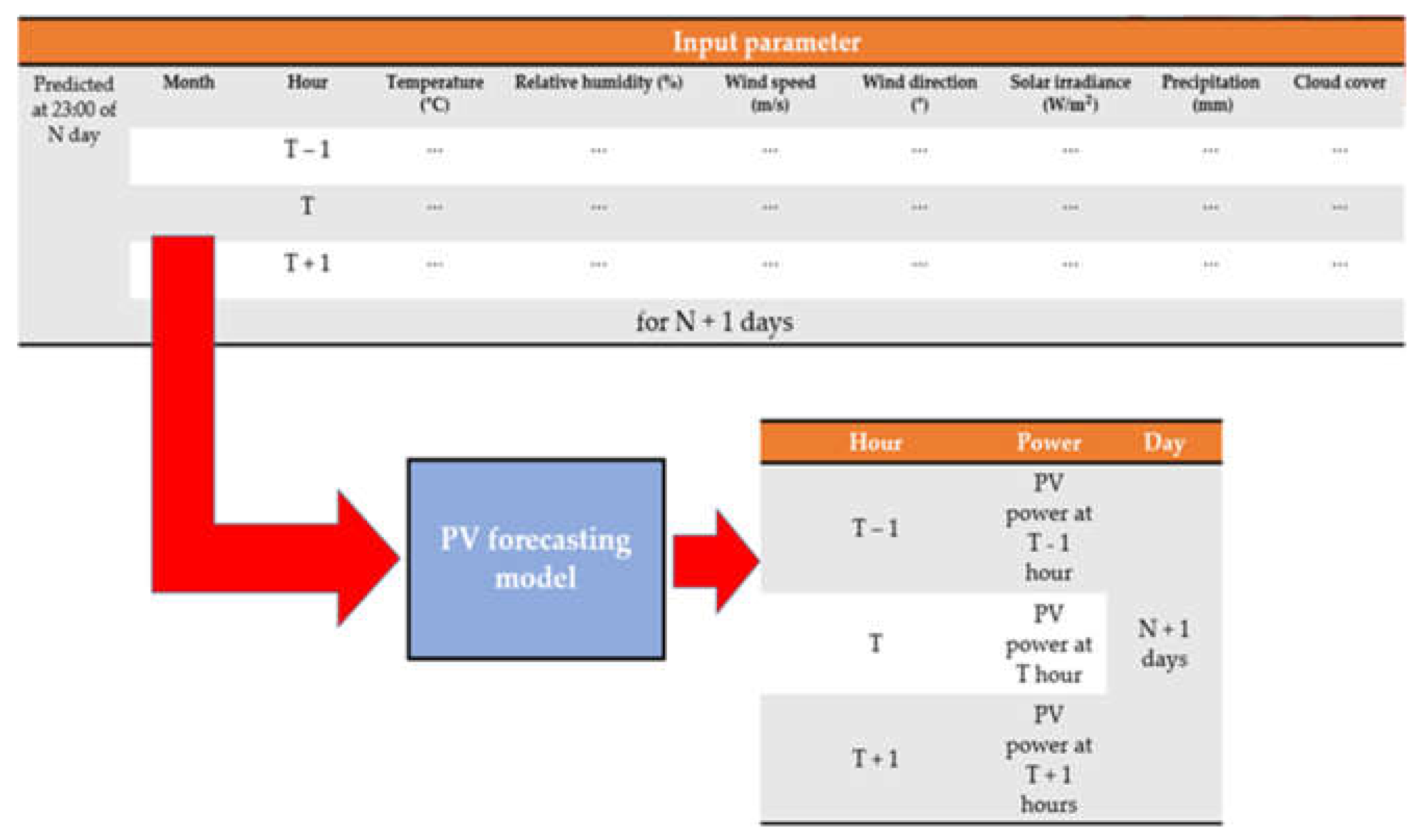
The relationship between the input and output data is shown in Figure 2. The meteorological data and the power generation data are 1-h time-step data, and the meteorological data predicted at 23:00 the day before are used for the PV generation prediction model for the next day. The PV forecasting is made on day N, and the forecasting model is used to calculate the hourly power generation of day N + 1. The time horizon depends on the time of the forecasting time, and it ranges from 1 h to a maximum of 25 h. For example, when the amount of power generated at 01:00 is predicted, the forecast is made at 23:00 on the day before, i.e., the forecast is made two hours ahead. In contrast, to estimate the power generation at 22:00, the forecast is made at 23:00 on the previous day. Here, we assume that the prediction of the next day’s power is made simultaneously with the release of the forecast data. Our prediction model was trained by 9 input features and 1 output dataset corresponding to year 2016, and it was validated by 9 input features and 1 output dataset corresponding to 2017. As shown in Figure 2, the 9 inputs are: month, hour, temperature (°C), relative humidity (%), wind speed (m/s), wind direction (°), solar irradiance (W/m2), precipitation (mm), and cloud cover. In the study, the missing data imputation was performed for all lossy data, and PV generation was predicted by means of SVR. The detailed theory and SVR optimization process are presented in [10]. In addition, we used the regression learner app in MATLAB R2018a software to implement and test the model. In the regression learner app, the median Gaussian SVM was selected as it affords the highest accuracy among SVR models. The median Gaussian SVM algorithm was executed on a computer with an Intel® Core™ i7-7700 CPU clocked at 3.60-GHz with 16.0 GB of RAM. Figure 3 depicts our power prediction model. In Figure 3, LI, MI, KNN, and MICE denote the linear interpolation, mode imputation, k-nearest neighbors, and multivariate imputation by chain equation algorithms, respectively. A more detailed description of the four methodologies is provided in Section 2.2.
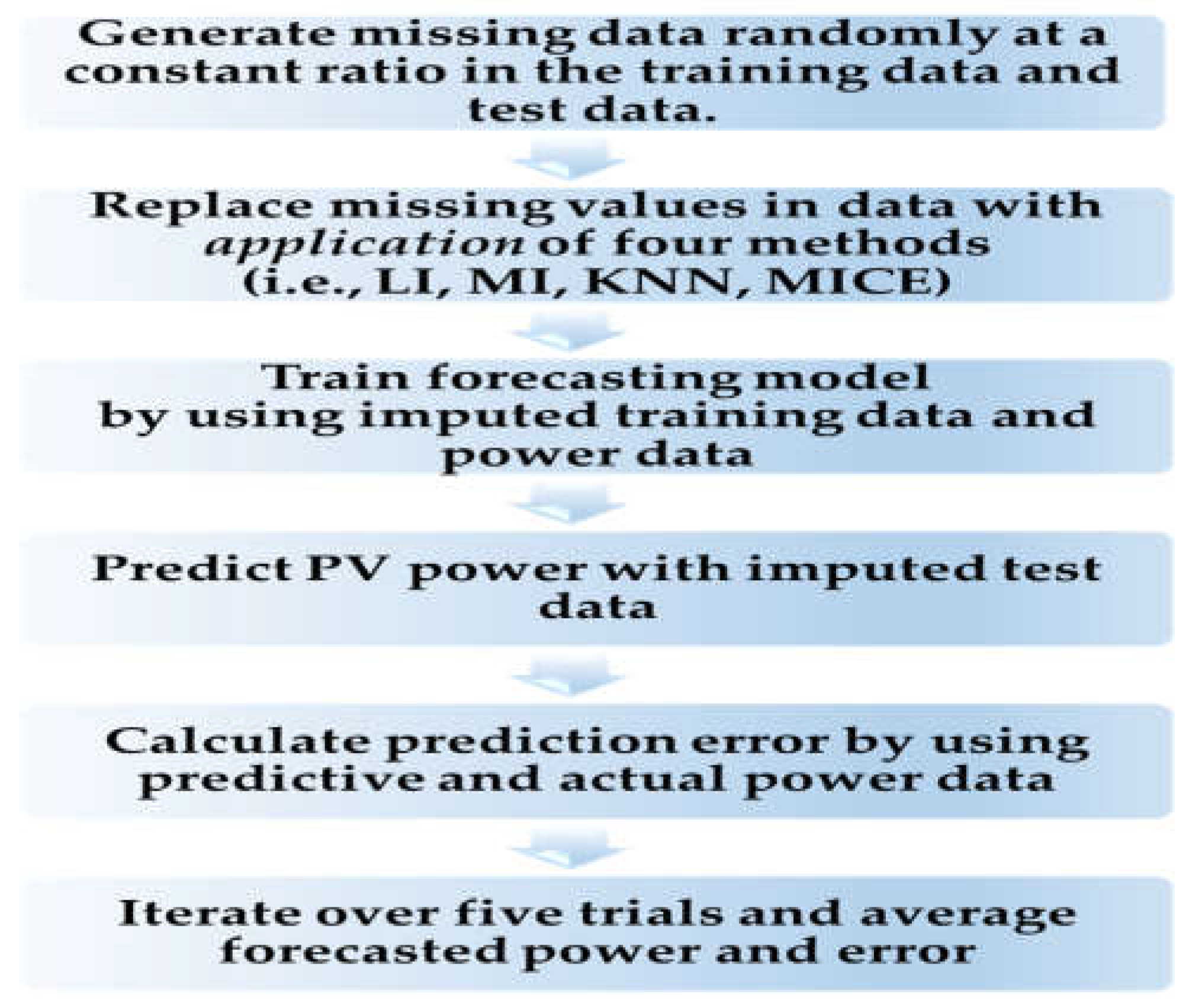
Further, Figure 4 depicts the simulation process of the proposed model.
2.2. Missing Data Imputation Methods
2.2.1. LI
LI is a method that replaces median missing data by using data at both ends of the data series. For example, let us consider the sequence of data samples shown in Figure 4, , with uniform sampling of function with step T.
In Figure 5, it is assumed that there is a linear relationship between data and data .
Thus, can be calculated by use of Equation (1) as below:
Likewise, other missing data can be filled by LI. This method is stable when missing data are sparse and discrete. Figure 5 depicts the structure of a hypothetical dataset with missing values. If the magnitude of n in a dataset is small, LI is easy, fast, affords accuracy, and provides smooth results. These criteria imply that there is a small amount of missing data. This also suggests that the LI is comparatively sound, since data are not likely to fluctuate rapidly in a short time frame. However, when the missing data interval lengths increase, the imputation accuracy degrades severely [22].
2.2.2. MI
MI is a method wherein missing data are replaced with the most frequently-observed data. It is one of the simplest missing data imputation approaches, wherein the mode forms the criterion of the central trend. It includes the fundamental data distribution in the dataset. Thus, we can select the most frequent numerical quantity to fill in the missing data, which makes the method simple and easy to apply. However, this method is unsuitable when there is a complicated relation between the data in the dataset [11]. In addition, there is a specific pattern for daily solar irradiance data based on the position of the Sun in the sky, which cannot be restored by a simple method such as MI. Nevertheless, we select this method in order to show that when the missing data are processed in an undesirable way, the prediction deviates drastically.
2.2.3. Imputation Using KNN
The KNN imputation is based on machine learning, which has been extensively used for classification, regression, and imputation [29]. The method considers the k most similar data of the uncompleted dataset [29,30,31,32]. In other words, these k-nearest neighbors aid in replacing missing data with estimates. Given a broken data pattern x, the method adopts the k-closest instances that are complete values in the features to be imputed (i.e., attributes with missing values in x) such that they decrease by a certain distance value as far as possible [29]. In our study, represents the set of KNN of x arranged in ascending order of distance. Although the KNN can be chosen for objects without missing values, it is also encouraged to substitute corrected data for missing data [30,32].
To process missing values with the use of KNN, let us suppose that x includes a missing value on the jth input feature. After its KNN are selected, we set , and the unknown value is estimated using the corresponding jth feature values of . If the jth input feature is a numerical or continuous variable, different estimation procedures can be implemented in the KNN approach. We weigh the contribution of each according to its distance to x, i.e., d(x, ), assigning higher weights to closer neighbors. The equation for the estimation of the values is given below.
where represents the weight related to the kth neighbor. A suitable option for corresponds to the inverse square of the distance, as described by Equation (3).
In this study, we use this weighted method to estimate missing values in the cases of numerical and distinct variables, and further, we arbitrarily set k = 3. It has been shown that this method is robust for missing data estimation [29,30,31,32]. Its primary limitation is that whenever the method searches for the most similar instances, the algorithm has to estimate the entire dataset. The method is particularly problematic for application to large databases because it is time consuming and computationally expensive for big data.
2.2.4. Multivariate Imputation by Chain Equations
The MICE algorithm designed by van Buuren and Groothuis-Oudshoorn [33] is based on a Markov chain Monte Carlo method wherein the state space is the collection of all imputed values [13]. The merit of MICE is that the results are computed after a comparatively few numbers of iterations. As per some studies [33,34], in general, five iterations are usually sufficient. The MICE algorithm [35] for the imputation of multivariate missing data consists of the following steps in Algorithm 1.
| Algorithm 1: MICE algorithm for imputation of multivariate missing data [35]. |
|
3. Impact Evaluation of Missing Data Imputation on PV Forecasting
In order to verify the effect of missing data imputation on PV forecasting, we used four error indices, root mean square error (RMSE), mean relative error (MRE), root mean square deviation (RMSD), and mean relative deviation (MRD), defined, respectively, as follows:
RMSE and MRE are performance errors of prediction models used in previous studies. RMSD and MRD are indicators that quantify the effect of the selected missing data imputation method on the PV power prediction model. Here, denotes the predicted PV power data without using missing data imputation. In other words, is the output predicted by the model trained with the initial weather data. We set as the predicted value and not the actual value in order to identify only the effect of missing data imputation. These indices are very different from the error metrics used in previous forecasting studies [8,9,10,23]. If is set as the actual output, the prediction error can be changed according to the forecast model and not the imputation method. Further, in the above equations, denotes the predicted value obtained with the application of missing data imputation, the PV power capacity, N the number of forecast PV power outputs, and the actual PV power. In this study, = 196 kWp. The RMSE and MRE can be calculated from these values. According to [9], RMSE indicates the average size of the error. A larger error corresponds to a larger weight being added to RMSE. The special importance of RMSE is that it indicates that the occurrence of a sudden large error is more problematic than multiple small errors occurring multiple times. Further, we use the MRE instead of the MAPE because a small real value can cause a large error. For example, in the case of the PV model, there is almost no solar power generation at 06:00, and the MAPE value is only measured for actual solar power generation. We therefore choose the error index of MRE.
4. Results and Discussion
4.1. Evaluation of PV Generation Forecasting Model Performance with Missing Data Imputation
The purpose of this study is to determine the degree to which the missing data imputation affects the PV forecasting. In practice, both the training data and test data can be applied to the missing data imputation method at the same time. However, if both datasets are used for missing data imputation simultaneously, it is difficult to understand which missing data imputation most affects the solar prediction. Therefore, we categorized the simulation into two cases: one is the case wherein the missing data imputation is applied only to the training dataset (Section 4.1.1), while the other is case wherein the missing data imputation is applied only to the test data (Section 4.1.2).
4.1.1. Evaluation of Forecasting Model Performance with Missing Data Imputation of Training Data
We used the weather dataset of 2017 for the forecast and 12 training weather datasets with missing values (2016) with three missing data rates and applied the four missing data imputation methods. The simulation process was as follows: First, we generated a conventional training dataset using the missing data rates (i.e., 10%, 15%, and 20%). Second, we replaced the missing values with new values obtained by use of each missing data imputation method. Third, we initiated progressive learning with the training dataset by application of the missing data imputation and test data. Lastly, we predicted the solar power generation for 24 h by means of the learned model. This set of steps forms one cycle that was repeated five times. Finally, we calculated the RMSD and MRD for each of the five predicted values. Here, the error was calculated from the predicted value of the trained model by use of the reference model predicted value and the data obtained using the missing value replacement method. The reference model refers to the trained model with the original training data and test data with no missing values.
Next, the values obtained with the iterations were averaged for each test period (i.e., 20–27 January, March, and June 2017) and missing data rates (10%, 15%, and 20%). The results corresponding to the prediction model error are listed in Table 1, while the deviation results are listed in Table 2, Table 3 and Table 4.
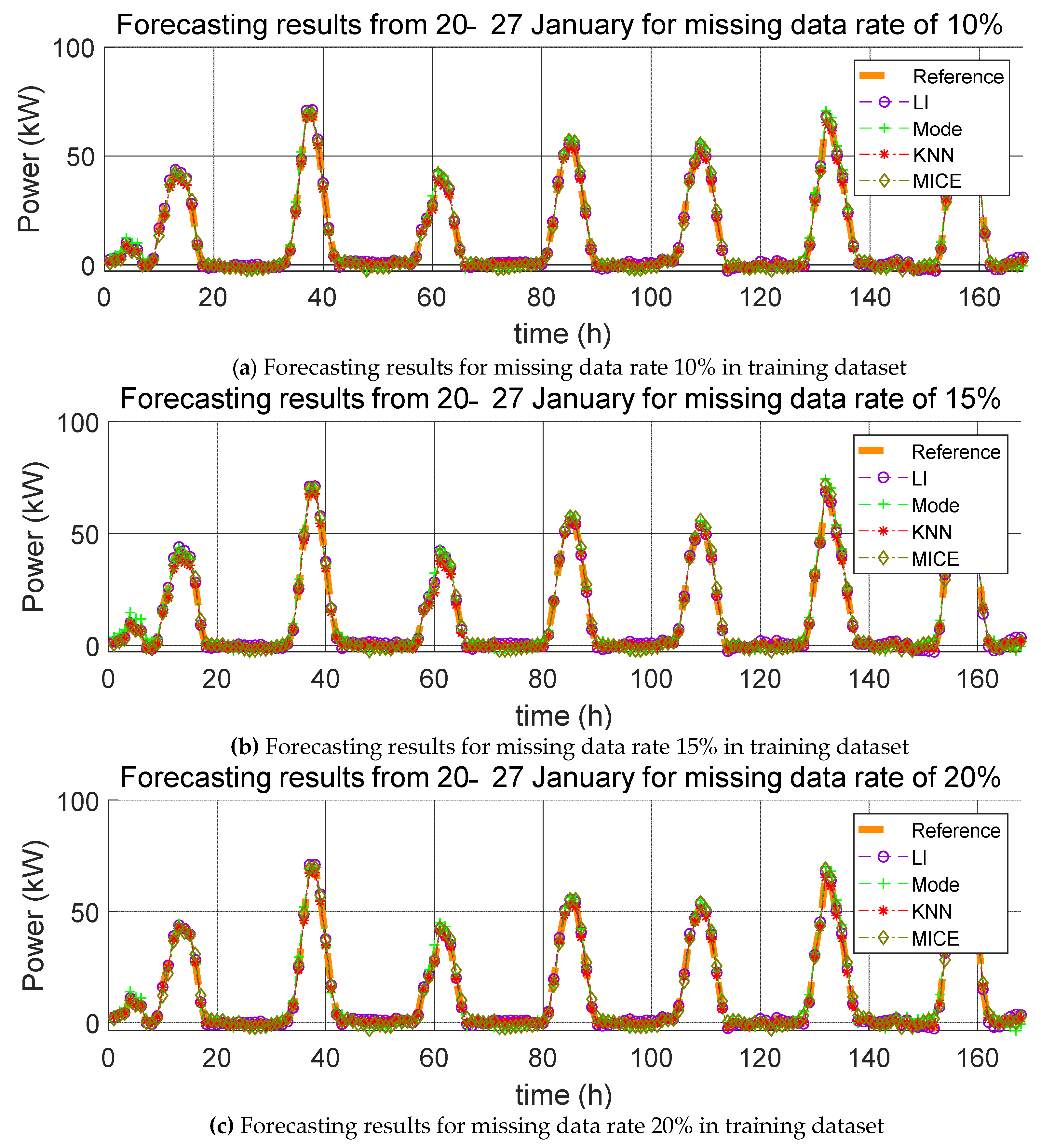
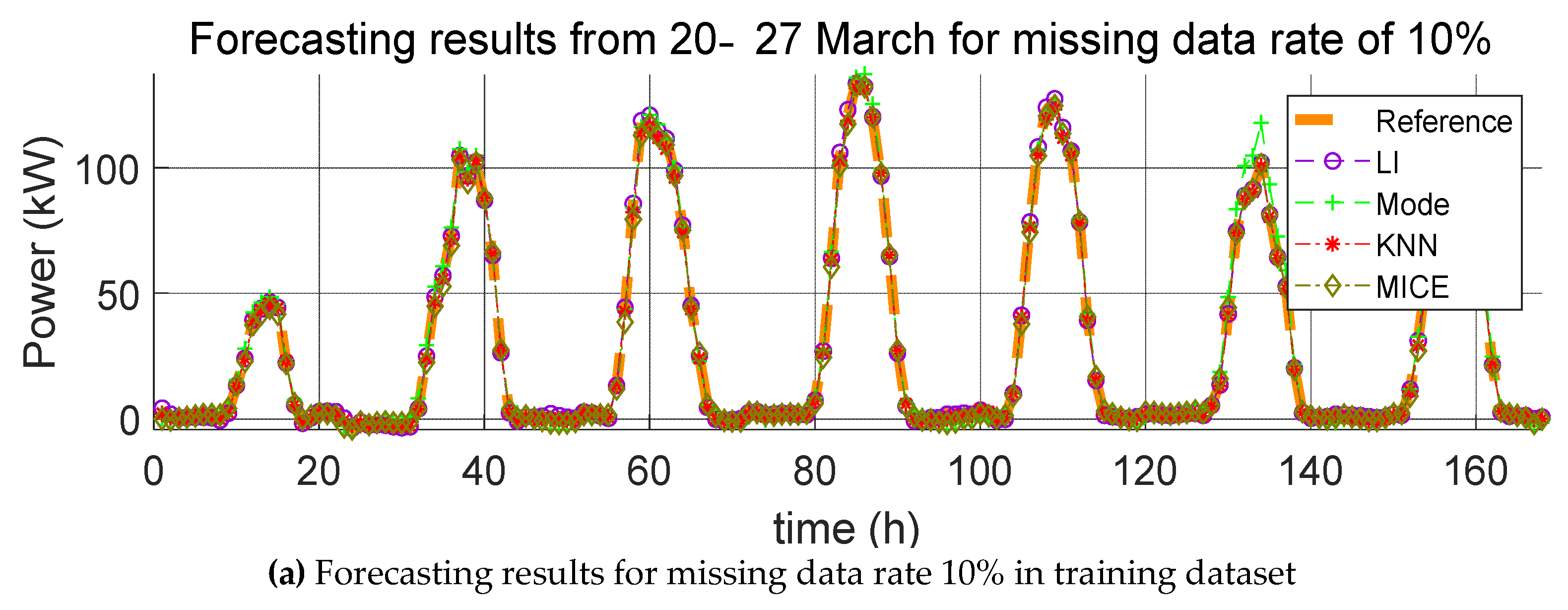
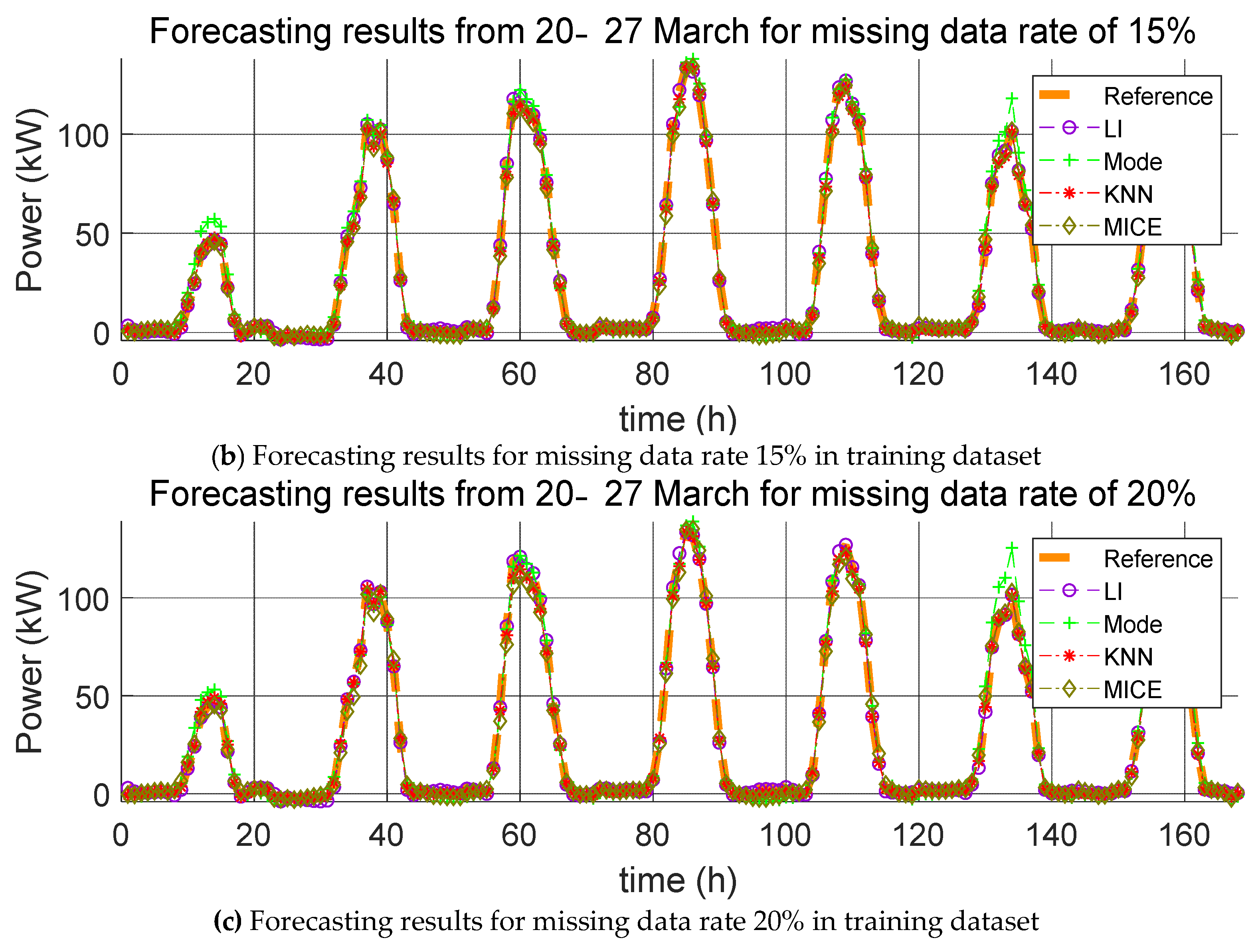
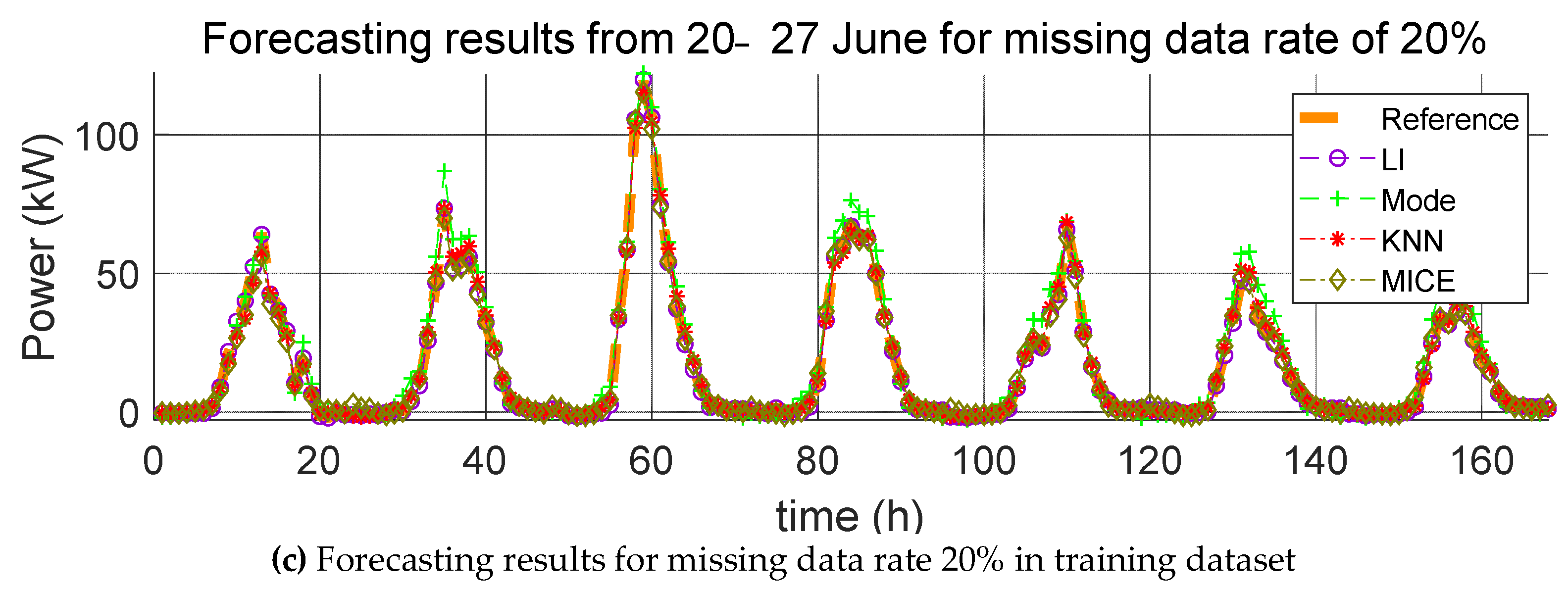
For each missing data rate, the graphs of the PV power generation prediction with the application of the four missing data imputation methods and the reference model are shown in Figure 6, Figure 7 and Figure 8. Here, the hourly predicted power generation values for each method are calculated as the average power generation values predicted through five iterations, and the reference model refers to the predicted model that is learned when no missing values are found in the training data and test data. Further, the average value of the power generation amount is the predicted power generation amount of five identical times generated in the five iterations. The average of the power generation values in the same time zone cannot be used to predict the power generation value every time because the positions where the missing values occur in the data are different even if the same missing value replacement method and prediction model are used. Therefore, we consider the averages of power generation in the same time zone and plot power generation profiles. This procedure also applies to Figure 9, Figure 10 and Figure 11.
4.1.2. Evaluation of Forecasting Model Performance with Missing Data Imputation for the Test Data Case
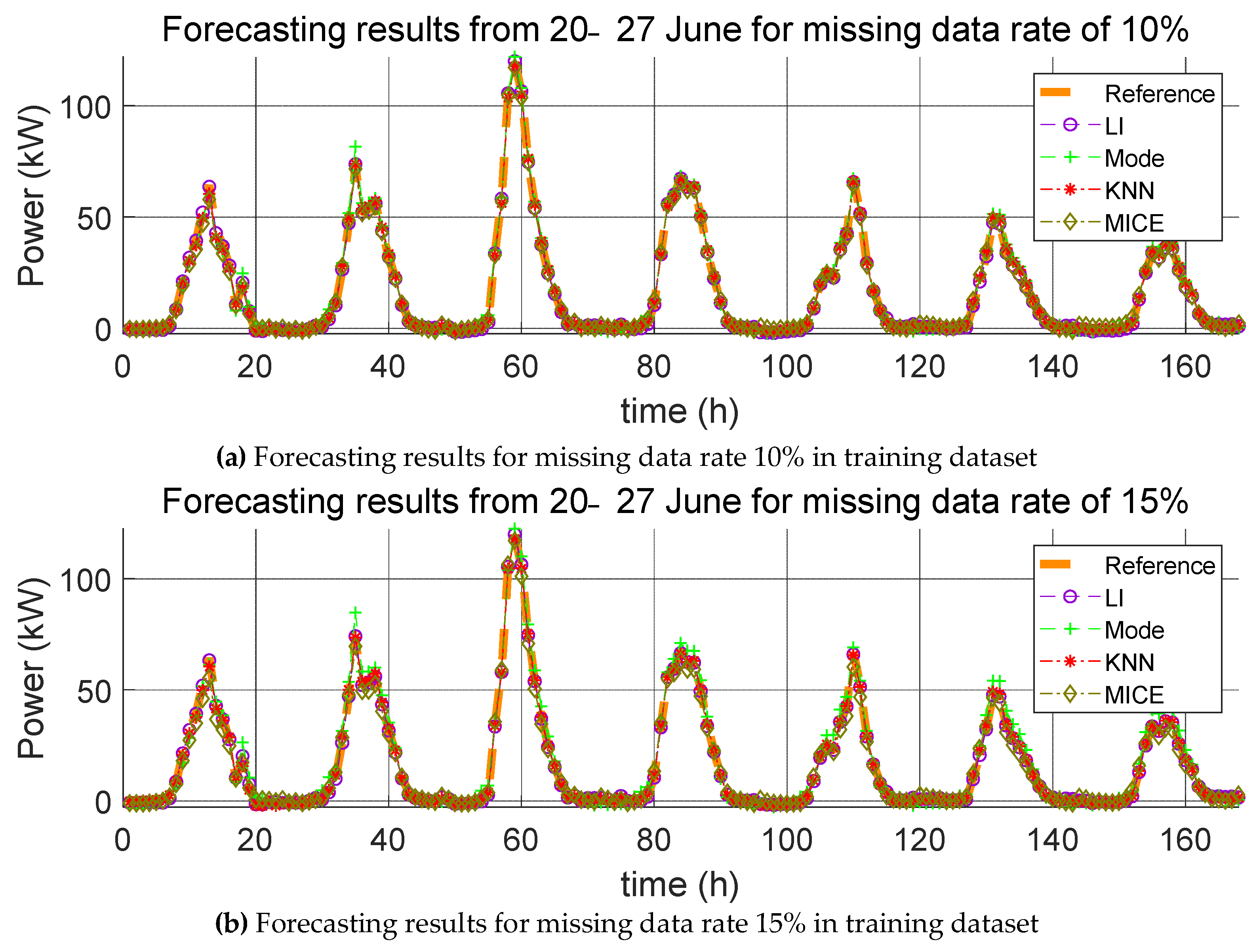
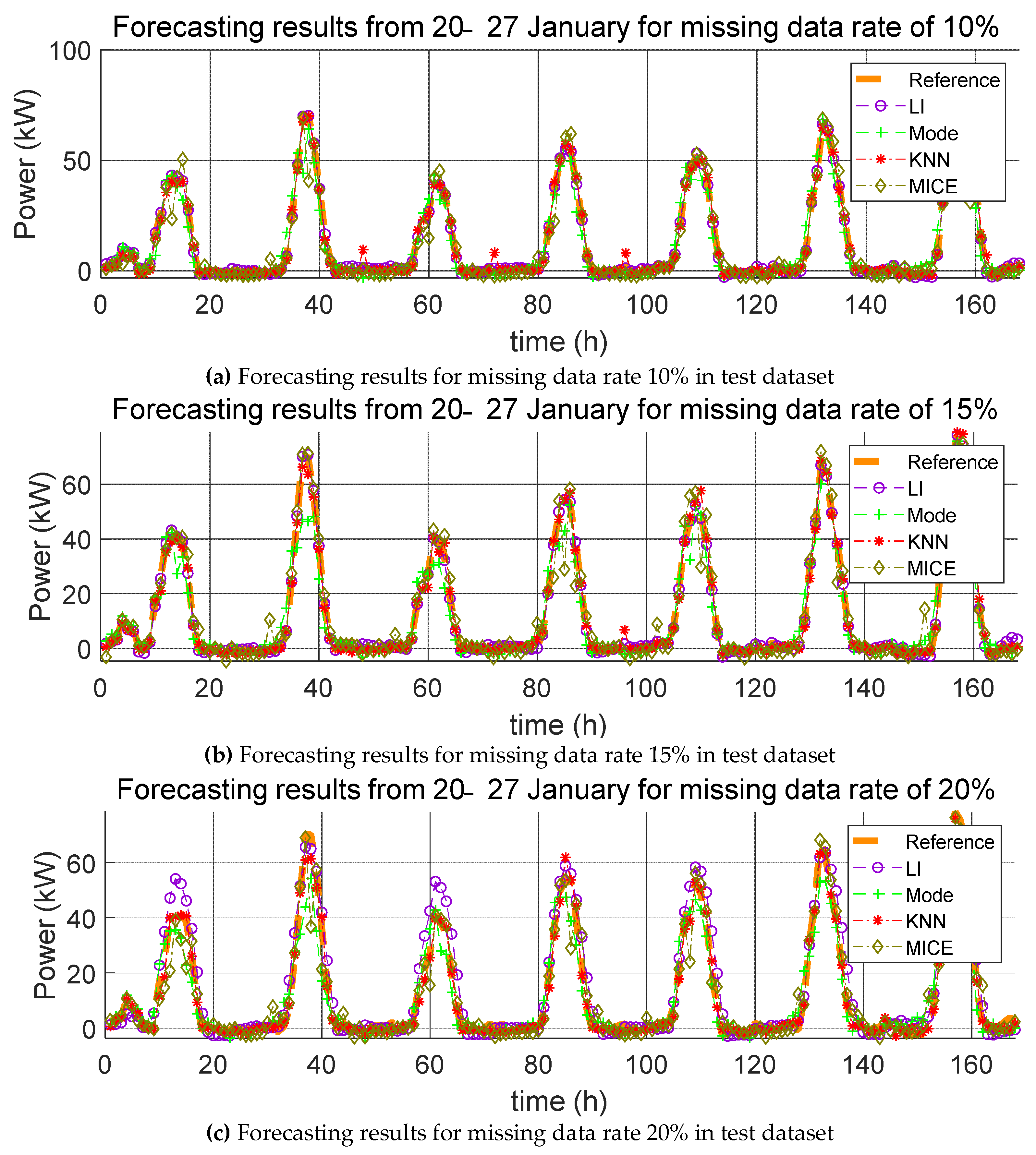
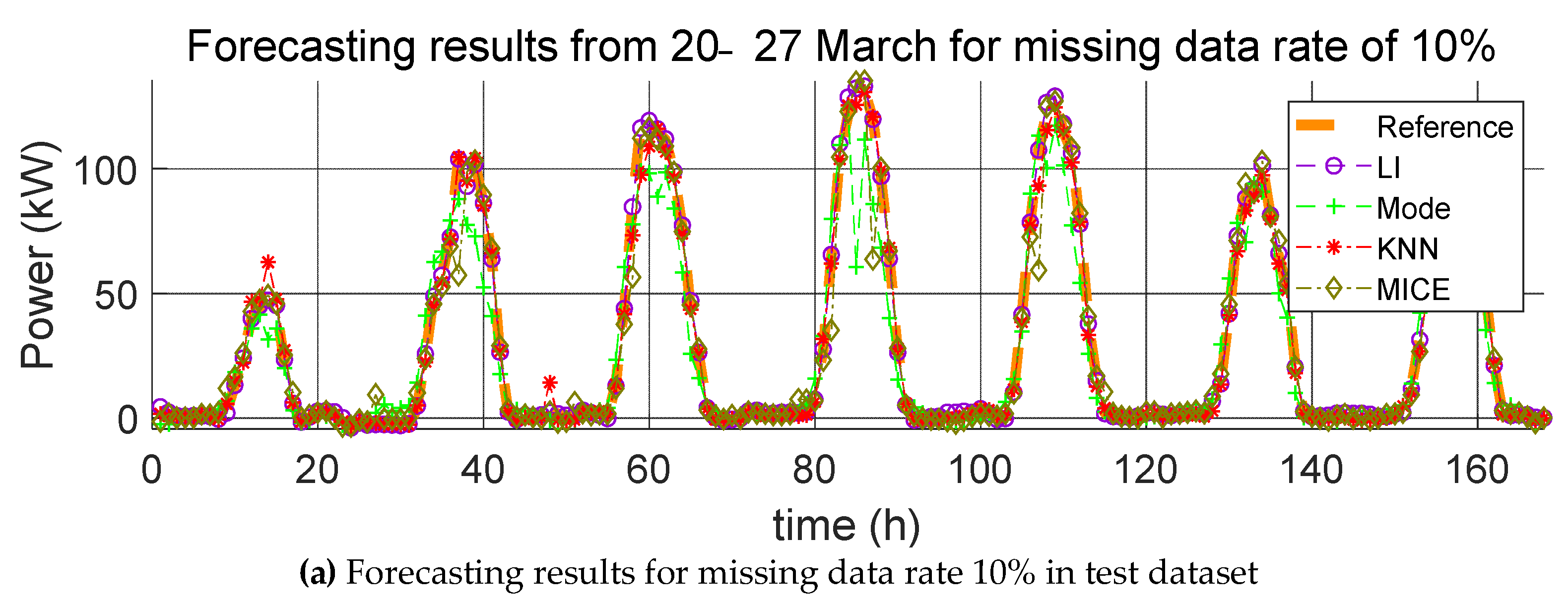
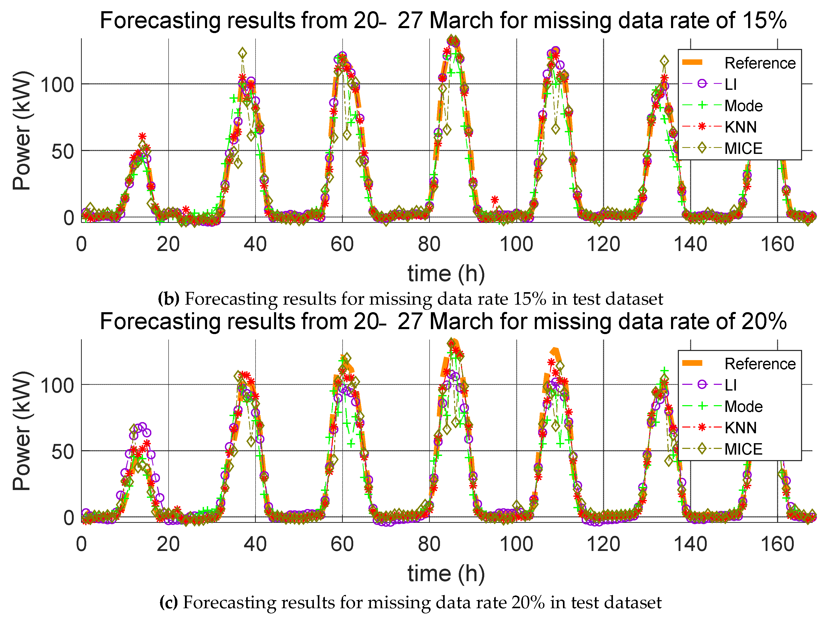
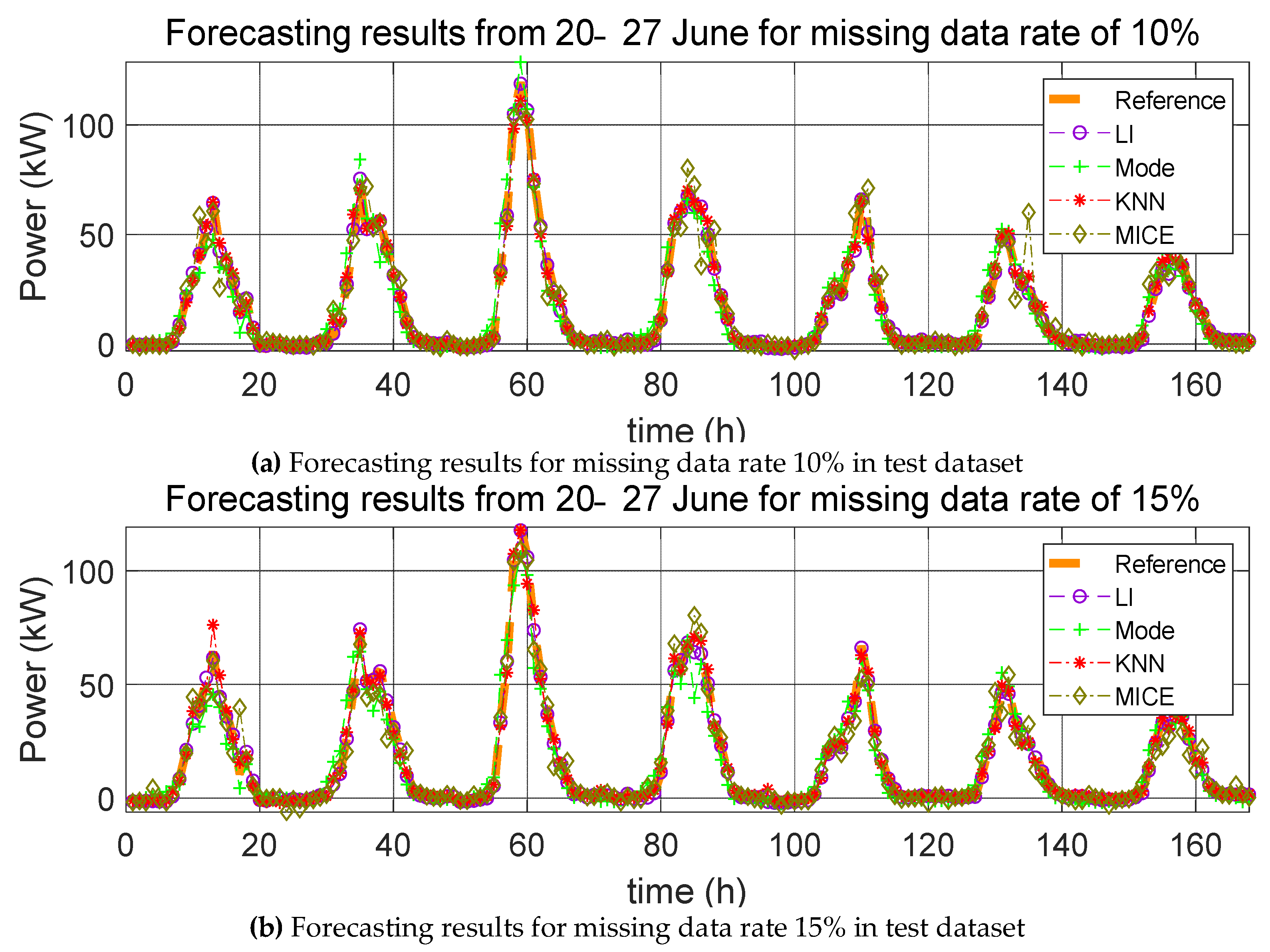
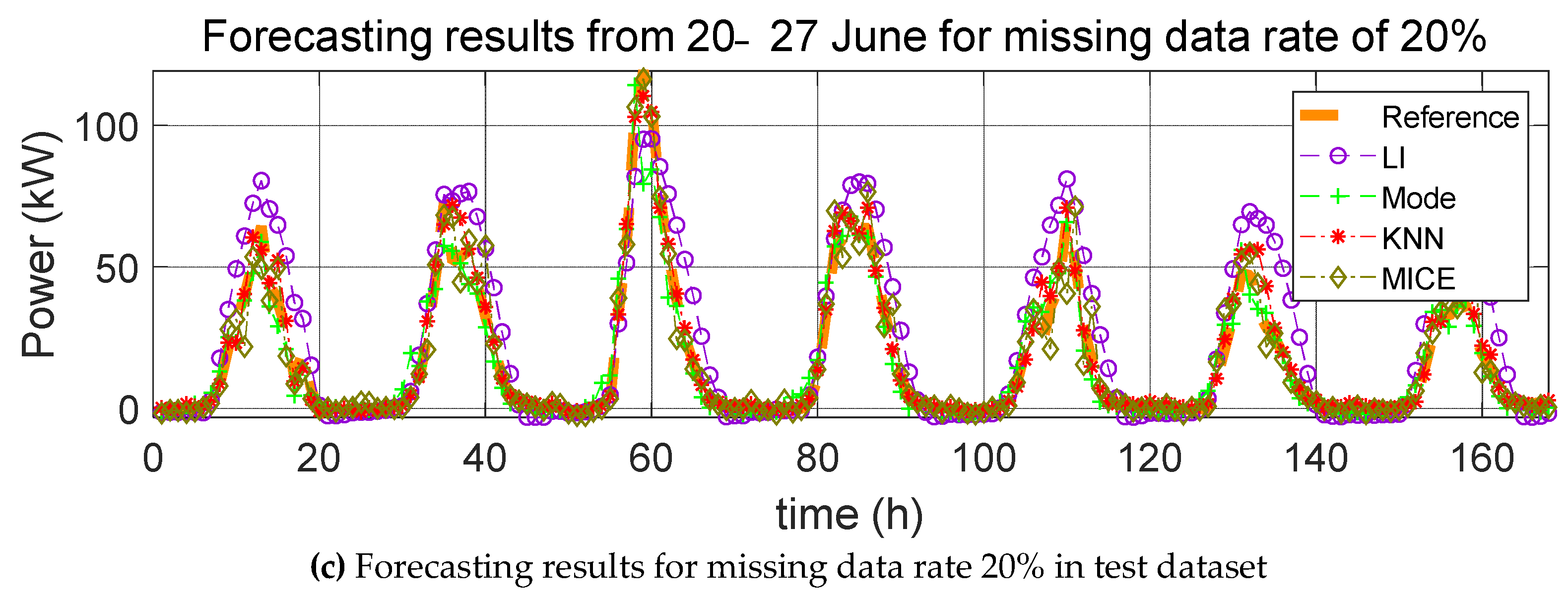
Here, we carry out the same process as that described in Section 4.1.1, except that the missing data are the test data and not the training data. The errors resulting from the estimation of the power generation with the application of the four missing data imputation methods according to the missing data rate with one training dataset are listed in Table 5, Table 6 and Table 7. As mentioned in Section 4.1.1, the mean value of the error was calculated over five trials, and the average of the predicted power generation was calculated by use of the four methods; the corresponding forecasting results are shown in Figure 9, Figure 10 and Figure 11.
4.2. Comparison of Methods and Discussion
PV prediction simulations were conducted for the case wherein the missing data imputation methods were applied to the training data and test data separately; the results for each of these cases have been presented in Section 4.1.1 and Section 4.1.2, respectively. When the missing data imputation method is applied to the training data, the RMSD is at most 5 kW and the MRD is less than 2%. That is, in this case, a large error does not occur when training is performed with data having no missing values. The reason underlying this result is as follows: first, the values for predicted power generation in this study correspond to the power generation values measured in 2017. However, this is not directly affected by the training data, which had missing values corresponding to 2016. Here, we note that the weather and PV generation data are time dependent data (i.e., time series data). The predicted value for PV generation in 2017 was determined by the 2017 training data alone. Accordingly, the 2016 weather data were only used to build the prediction model and did not directly impact the data generated for 2017. Second, even if the missing data rate is at most 20%, the training model is more influenced by the remaining 80% training data, and not the 20% missing data. Therefore, although missing data occur in the training data, there is no noticeably large error.
On the other hand, there is a noticeable difference between when the missing data imputation method is applied to the test data and when this method is not applied. Because the test data correspond to 2017, the predicted values for 2017 are directly affected. For example, the PV power generation prediction for 20 January 2017 was determined using meteorological data, such as solar radiation, temperature, and precipitation, as well as predicted time of day. Since the independent to dependent variable relationship is established between data of the same time, the value for the predicted PV power generation changes as values for the weather data are changed. From Table 5, Table 6 and Table 7, it can be observed that the error between the reference model and predicted model with missing data imputation increases with increasing missing data rates. When the missing data rate is low, LI affords the least error. However, for high missing data rates, the KNN method yields the smallest error. As the missing data rate increases, the amount of adjoining missing values increases in the datasets. LI is suitable for missing value imputations at a specific point in time, but it is not accurate for missing values in successive sections. Thus, when the missing data rate is 20%, the error of LI rapidly increases. MI yields the largest error value regardless of the missing data rate and test duration. This method is suitable for discrete data; however, weather data are continuous data. In conclusion, these simulations indicate that the KNN method is the most suitable missing data imputation method for day-ahead PV power forecasting.
5. Conclusions
The prediction of PV power generation is important in situations wherein the number of new and renewable power generation systems joining the grid increases. In this regard, many machine learning-based methods for power generation prediction have been studied and utilized. In order to ensure increased accuracy, it is required to compensate for missing meteorological data values suitably. In this study, we studied four methods to fill in missing values in PV power generation prediction: LI, MI, the statistical missing data imputation method MICE, and the machine learning-based KNN. In order to test these methods, we chose the SVR model as the solar power prediction model and applied the four methods to the SVR model. We used the indices of RMSD (kW) and MRD (%) to calculate the degree of difference between the predicted value with and without the application of missing data imputation. Four different predictions were obtained for each missing data imputation method. We next obtained the error for each method over five trials to evaluate the performance of each missing data imputation method. When the missing data imputation is applied to PV power forecasting, the missing training data do not affect PV power prediction. However, missing test data considerably affect PV power prediction. Further, the error in the case that the missing data rate is less than 15% is lowest with the LI method, but for missing data rates of 20% or more, the KNN method outperforms the LI method. Moreover, the error obtained with KNN application is relatively low compared with that obtained with the LI method, since the error rate is reflected by the missing data rate. This result implies that the difference between the reference model and the prediction model with missing data imputation is the smallest for the KNN method. Therefore, the best result is obtained by processing missing weather data with the use of KNN. In summary, we believe that our findings can significantly contribute to accurate PV power generation forecasting.
Author Contributions
T.K. conceived of the idea for the research and preformed the simulations as the first author. W.K. provided comments on the modeling and analysis. J.K. led and supervised the research and is the corresponding author.
Funding
This research received no external funding.
Acknowledgments
This work was supported by the Korea Institute of Energy Technology Evaluation and Planning (KETEP) and the Ministry of Trade, Industry & Energy (MOTIE) of the Republic of Korea (No. 20181210301380).
Conflicts of Interest
The authors declare no conflict of interest.
References
- Highlights of the REN21 Renewables 2018 Global Status Report in Perspective. 2018. Available online: http://www.ren21.net/wp-content/uploads/2018/06/17-8652_GSR2018_FullReport_web_final_.pdf (accessed on 17 August 2018).
- Trends 2016 in Photovoltaic Applications. Available online: http://www.iea-pvps.org/fileadmin/dam/public/report/national/Trends_2016_-_mr.pdf (accessed on 17 August 2018).
- Yang, D.; Kleissl, J.; Gueymard, C.A.; Pedro, H.T.; Coimbra, C.F. History and trends in solar irradiance and PV power forecasting: A preliminary assessment and review using text mining. Sol. Energy 2018, 168, 60–101. [Google Scholar] [CrossRef]
- Panapakidis, I.; Bouhouras, A.; Christoforidis, G. A missing data treatment method for photovoltaic installations. In Proceedings of the IEEE International Energy Conference (ENERGYCON), Limassol, Cyprus, 3–7 June 2018; pp. 1–6. [Google Scholar]
- Batista, G.; Monard, M. An analysis of four missing data treatment methods for supervised learning. Appl. Artif. Intell. 2003, 17, 519–533. [Google Scholar] [CrossRef]
- Banks, D.; McMorris, F.; Arabie, P.; Gaul, W. Classification, Clustering, and Data Mining Applications; Springer: Berlin/Heidelberg, Germany, 2004; pp. 639–647. ISBN 978-3-642-17103-1. [Google Scholar]
- Luengo, J.; Garcia, S.; Herrera, F. A study on the use of imputation methods for experimentation with Radial Basis Function Network classifiers handling missing attribute values: The good synergy between RBFNs and EventCovering method. Neural Netw. 2010, 23, 406–418. [Google Scholar] [CrossRef] [PubMed]
- Shi, J.; Lee, W.-J.; Liu, Y.; Yang, Y.; Wang, P. Forecasting power output of photovoltaic systems based on weather classification and support vector machines. IEEE Trans. Ind. Appl. 2012, 48, 1064–1069. [Google Scholar] [CrossRef]
- Yang, H.-T.; Huang, C.-M.; Huang, Y.-C.; Pai, Y.-S. A weather-based hybrid method for 1-day ahead hourly forecasting of PV power output. IEEE Trans. Sustain. Energy 2014, 5, 917–926. [Google Scholar] [CrossRef]
- Das, U.K.; Tey, K.S.; Seyedmahmoudian, M.; Idna Idris, M.Y.; Mekhilef, S.; Horan, B.; Stojcevski, A. SVR-based model to forecast PV power generation under different weather conditions. Energies 2017, 10, 876. [Google Scholar] [CrossRef]
- Xu, X.; Chong, W.; Li, S.; Arabo, A.; Xiao, J. MIAEC: Missing data imputation based on the evidence chain. IEEE Access 2018, 6, 12983–12992. [Google Scholar] [CrossRef]
- Sovilj, D.; Eirola, E.; Miche, Y.; Björk, K.-M.; Nian, R.; Akusok, A.; Lendasse, A. Extreme learning machine for missing data using multiple imputations. Neurocomputing 2016, 174, 220–231. [Google Scholar] [CrossRef]
- Turrado, C.C.; López, M.D.C.M.; Lasheras, F.S.; Gómez, B.A.R.; Rollé, J.L.C.; Juez, F.J.d.C. Missing data imputation of solar radiation data under different atmospheric conditions. Sensors 2014, 14, 20382–20399. [Google Scholar] [CrossRef] [PubMed]
- Layanun, V.; Suksamosorn, S.; Songsiri, J. Missing-data imputation for solar irradiance forecasting in Thailand. In Proceedings of the 56th Annual Conference of the Society of Instrument and Control Engineers of Japan (SICE), Kanazawa, Japan, 19–22 September 2017. [Google Scholar]
- Yozgatligil, C.; Aslan, S.; Iyigun, C.; Batmaz, I. Comparison of missing value imputation methods in time series: The case of Turkish meteorological data. Theor. Appl. Climatol. 2013, 112, 143–167. [Google Scholar] [CrossRef]
- Riza, D.; Gilani, S.; Aris, M. Hourly Solar Radiation Estimation Using Ambient Temperature and Relative Humidity Data. Int. J. Environ. Sci. Dev. 2011, 2, 188–193. [Google Scholar] [CrossRef]
- Teegavarapu, R.S.V.; Chandramouli, V. Improved weighting methods, deterministic and stochastic data-driven models for estimation of missing precipitation records. J. Hydrol. 2005, 312, 191–206. [Google Scholar] [CrossRef]
- Teegavarapu, R.S.V.; Tufail, M.; Ormsbee, L. Optimal functional forms for estimation of missing precipitation data. J. Hydrol. 2009, 374, 106–115. [Google Scholar] [CrossRef]
- Kim, J.-W.; Pachepsky, Y.A. Reconstructing missing daily precipitation data using regression trees and artificial neural networks for SWAT streamflow simulation. J. Hydrol. 2010, 394, 305–314. [Google Scholar] [CrossRef]
- Campozano, L.; Sánchez, E.; Avilés, A.; Samaniego, E. Evaluation of infilling methods for time series of daily precipitation and temperature: The case of the Ecuadorian Andes. Maskana 2014, 5, 99–115. [Google Scholar]
- Jerez, J.M.; Molina, I.; García-Laencina, P.J.; Alba, E.; Ribelles, N.; Martín, M.; Franco, L. Missing data imputation using statistical and machine learning methods in a real breast cancer problem. Artif. Intell. Med. 2010, 50, 105–115. [Google Scholar] [CrossRef] [PubMed]
- Laña, I.; Olabarrieta, I.I.; Vélez, M.; Del Ser, J. On the imputation of missing data for road traffic forecasting: New insights and novel techniques. Transp. Res. Part C Emerg. Technol. 2018, 90, 18–33. [Google Scholar] [CrossRef]
- Shireen, T.; Shao, C.; Wang, H.; Li, J.; Zhang, X.; Li, M. Iterative multi-task learning for time-series modeling of solar panel PV outputs. Appl. Energy 2018, 212, 654–662. [Google Scholar] [CrossRef]
- Crespo Turrado, C.; Sánchez Lasheras, F.; Calvo-Rollé, J.L.; Piñón-Pazos, A.J.; de Cos Juez, F.J. A new missing data imputation algorithm applied to electrical data loggers. Sensors 2015, 15, 31069–31082. [Google Scholar] [CrossRef]
- Open Data Portal. Available online: https://www.data.go.kr/dataset/15000962/fileData.do (accessed on 17 August 2017).
- Weather Open Data Portal. Available online: https://data.kma.go.kr/data/rmt/rmtList.do?code=400&pgmNo=570 (accessed on 17 August 2017).
- Holmgren, W.F.; Groenendyk, D.G. An open source solar power forecasting tool using PVLIB-Python. In Proceedings of the IEEE 43rd Photovoltaic Specialists Conference (PVSC), Portland, OR, USA, 5–10 June 2016; pp. 972–975. [Google Scholar]
- Summary on Solar Measurement. Available online: https://www.ammonit.com/en/wind-solar-wissen/solarmessung#top (accessed on 25 November 2018).
- García-Laencina, P.J.; Sancho-Gómez, J.-L.; Figueiras-Vidal, A.R.; Verleysen, M. K nearest neighbours with mutual information for simultaneous classification and missing data imputation. Neurocomputing 2009, 72, 1483–1493. [Google Scholar] [CrossRef] [Green Version]
- Batista, G.E.; Monard, M.C. A study of K-nearest neighbour as an imputation method. HIS 2002, 87, 48. [Google Scholar]
- Hruschka, E.R.; Hruschka, E.R.; Ebecken, N.F. Towards efficient imputation by nearest-neighbors: A clustering-based approach. In Proceedings of the Australasian Joint Conference on Artificial Intelligence, Cairns, Australia, 4–6 December 2004; Springer: Berlin/Heidelberg, Germany, 2004; pp. 513–525. [Google Scholar]
- Troyanskaya, O.; Cantor, M.; Sherlock, G.; Brown, P.; Hastie, T.; Tibshirani, R.; Botstein, D.; Altman, R.B. Missing value estimation methods for DNA microarrays. Bioinformatics 2001, 17, 520–525. [Google Scholar] [CrossRef] [PubMed] [Green Version]
- Buuren, S.v.; Groothuis-Oudshoorn, K. mice: Multivariate imputation by chained equations in R. J. Stat. Softw. 2010, 45, 1–68. [Google Scholar] [CrossRef]
- Müller, K.-R.; Smola, A.J.; Rätsch, G.; Schölkopf, B.; Kohlmorgen, J.; Vapnik, V. Predicting time series with support vector machines. In Proceedings of the International Conference on Artificial Neural Networks, Lausanne, Switzerland, 8–10 October 1997; Springer: Berlin/Heidelberg, Germany, 1997; pp. 999–1004. [Google Scholar] [Green Version]
- Azur, M.J.; Stuart, E.A.; Frangakis, C.; Leaf, P.J. Multiple imputation by chained equations: What is it and how does it work? Int. J. Methods Psychiatr. Res. 2011, 20, 40–49. [Google Scholar] [CrossRef] [PubMed]
Figure 1.
Global solar photovoltaic capacity and annual additions from 2007–2017.

Figure 2.
Time step of data and time horizon of the forecasting model.

Figure 3.
Support vector regression (SVR)-based photovoltaic (PV) power prediction model utilizing missing data imputation. LI, linear interpolation; MI, mode imputation; MICE, multivariate imputation by chain equation.
Figure 3.
Support vector regression (SVR)-based photovoltaic (PV) power prediction model utilizing missing data imputation. LI, linear interpolation; MI, mode imputation; MICE, multivariate imputation by chain equation.

Figure 4.
Process of the simulation for PV forecasting model.

Figure 5.
Datasets with missing data.

Figure 6.
Forecasting results from 20–27 January for various missing data rates (10%, 15%, and 20%).
Figure 6.
Forecasting results from 20–27 January for various missing data rates (10%, 15%, and 20%).

Figure 7.
Forecasting results from 20–27 March for various missing data rates (10%, 15%, and 20%).


Figure 8.
Forecasting results from 20–27 June for various missing data rates (10%, 15%, and 20%).


Figure 9.
Forecasting results from 20–27 January for various missing data rates (10%, 15%, and 20%).
Figure 9.
Forecasting results from 20–27 January for various missing data rates (10%, 15%, and 20%).

Figure 10.
Forecasting results from 20–27 March for various missing data rates (10%, 15%, and 20%).


Figure 11.
Forecasting results from 20–27 June for various missing data rates (10%, 15%, and 20%).


Table 1.
Error of PV forecasting reference model.
| Month | RMSE (kW) | MRE (%) |
|---|---|---|
| 1 | 18.08 | 5.07 |
| 3 | 31.12 | 8.86 |
| 6 | 18.96 | 5.27 |
Table 2.
Deviation of missing data imputation from the PV forecasting model in January using the test set. MRD, mean relative deviation;
Table 2.
Deviation of missing data imputation from the PV forecasting model in January using the test set. MRD, mean relative deviation;
| Missing Data Rate | 10% | 15% | 20% | |||
|---|---|---|---|---|---|---|
| Method | RMSD (kW) | MRD (%) | RMSD (kW) | MRD (%) | RMSD (kW) | MRD (%) |
| LI | 0.46 | 0.17 | 0.67 | 0.27 | 0.60 | 0.23 |
| MI | 2.14 | 3.49 | 2.42 | 0.97 | 2.69 | 1.41 |
| KNN | 1.05 | 0.40 | 1.55 | 0.61 | 1.07 | 0.46 |
| MICE | 1.70 | 0.73 | 2.07 | 0.87 | 2.21 | 0.93 |
| Average | 1.63 | 1.20 | 1.68 | 0.68 | 1.64 | 0.76 |
Table 3.
Deviation of missing data imputation from the PV forecasting model in March using the test set.
Table 3.
Deviation of missing data imputation from the PV forecasting model in March using the test set.
| Missing Data Rate | 10% | 15% | 20% | |||
|---|---|---|---|---|---|---|
| Method | RMSD (kW) | MRD (%) | RMSD (kW) | MRD (%) | RMSD (kW) | MRD (%) |
| LI | 0.44 | 0.18 | 0.54 | 0.22 | 0.57 | 0.23 |
| MI | 3.49 | 1.20 | 3.94 | 1.41 | 4.95 | 1.68 |
| KNN | 1.43 | 0.52 | 2.24 | 0.74 | 1.84 | 0.65 |
| MICE | 1.70 | 0.73 | 2.07 | 0.87 | 3.32 | 1.20 |
| Average | 1.77 | 0.66 | 2.20 | 0.81 | 2.67 | 0.94 |
Table 4.
Deviation of missing data imputation from the PV forecasting model in June using the test set.
Table 4.
Deviation of missing data imputation from the PV forecasting model in June using the test set.
| Missing Data Rate | 10% | 15% | 20% | |||
|---|---|---|---|---|---|---|
| Method | RMSD (kW) | MRD (%) | RMSD (kW) | MRD (%) | RMSD (kW) | MRD (%) |
| LI | 0.41 | 0.16 | 0.57 | 0.24 | 0.52 | 0.19 |
| MI | 1.99 | 0.78 | 3.11 | 1.20 | 4.60 | 1.67 |
| KNN | 1.01 | 0.41 | 1.03 | 0.39 | 1.78 | 0.63 |
| MICE | 1.53 | 0.60 | 2.36 | 0.89 | 1.80 | 0.65 |
| Average | 1.24 | 0.49 | 1.77 | 0.68 | 2.18 | 0.79 |
Table 5.
Deviation of missing data imputation from the PV forecasting model with test data in January.
Table 5.
Deviation of missing data imputation from the PV forecasting model with test data in January.
| Missing Data Rate | 10% | 15% | 20% | |||
|---|---|---|---|---|---|---|
| Method | RMSD (kW) | MRD (%) | RMSD (kW) | MRD (%) | RMSD (kW) | MRD (%) |
| LI | 0.67 | 0.23 | 0.86 | 0.30 | 9.04 | 3.27 |
| MI | 8.89 | 2.76 | 9.47 | 2.81 | 11.37 | 3.48 |
| KNN | 3.97 | 1.15 | 4.05 | 1.16 | 5.75 | 1.75 |
| MICE | 6.37 | 1.74 | 5.80 | 1.74 | 7.25 | 2.28 |
| Average | 4.98 | 1.47 | 5.05 | 1.50 | 8.35 | 2.70 |
Table 6.
Deviation of missing data imputation from the PV forecasting model with test data in March.
Table 6.
Deviation of missing data imputation from the PV forecasting model with test data in March.
| Missing Data Rate | 10% | 15% | 20% | |||
|---|---|---|---|---|---|---|
| Method | RMSD (kW) | MRD (%) | RMSD (kW) | MRD (%) | RMSD (kW) | MRD (%) |
| LI | 1.41 | 0.42 | 1.43 | 0.53 | 15.69 | 5.30 |
| MI | 21.83 | 6.30 | 17.46 | 5.32 | 22.42 | 6.26 |
| KNN | 6.36 | 1.61 | 6.05 | 1.94 | 11.37 | 3.05 |
| MICE | 13.26 | 2.75 | 13.66 | 3.39 | 14.82 | 3.67 |
| Average | 10.72 | 2.77 | 9.65 | 2.80 | 16.08 | 4.57 |
Table 7.
Deviation of missing data imputation from the PV forecasting model with test data in June.
| Missing Data Rate | 10% | 15% | 20% | |||
|---|---|---|---|---|---|---|
| Method | RMSD (kW) | MRD (%) | RMSD (kW) | MRD (%) | RMSD (kW) | MRD (%) |
| LI | 1.00 | 0.33 | 1.11 | 0.41 | 24.33 | 8.70 |
| MI | 9.13 | 3.11 | 9.72 | 3.34 | 10.86 | 3.38 |
| KNN | 3.69 | 1.06 | 4.79 | 1.42 | 6.65 | 1.89 |
| MICE | 7.24 | 1.99 | 5.84 | 1.93 | 8.41 | 2.36 |
| Average | 5.27 | 1.62 | 5.37 | 1.78 | 12.56 | 4.08 |
© 2019 by the authors. Licensee MDPI, Basel, Switzerland. This article is an open access article distributed under the terms and conditions of the Creative Commons Attribution (CC BY) license (http://creativecommons.org/licenses/by/4.0/).
Share and Cite
MDPI and ACS Style
Kim, T.; Ko, W.; Kim, J. Analysis and Impact Evaluation of Missing Data Imputation in Day-ahead PV Generation Forecasting. Appl. Sci. 2019, 9, 204. https://0-doi-org.brum.beds.ac.uk/10.3390/app9010204
AMA Style
Kim T, Ko W, Kim J. Analysis and Impact Evaluation of Missing Data Imputation in Day-ahead PV Generation Forecasting. Applied Sciences. 2019; 9(1):204. https://0-doi-org.brum.beds.ac.uk/10.3390/app9010204
Chicago/Turabian StyleKim, Taeyoung, Woong Ko, and Jinho Kim. 2019. "Analysis and Impact Evaluation of Missing Data Imputation in Day-ahead PV Generation Forecasting" Applied Sciences 9, no. 1: 204. https://0-doi-org.brum.beds.ac.uk/10.3390/app9010204
Note that from the first issue of 2016, this journal uses article numbers instead of page numbers. See further details here.